Detrended fluctuation analysis of power-law-correlated sequences with random noises
Abstract
Improvement in time resolution sometimes introduces short-range random noises into temporal data sequences. These noises affect the results of power-spectrum analyses and the Detrended Fluctuation Analysis (DFA). The DFA is one of useful methods for analyzing long-range correlations in non-stationary sequences. The effects of noises are discussed based on artificial temporal sequences. Short-range noises prevent power-spectrum analyses from detecting long-range correlations. The DFA can extract long-range correlations from noisy time sequences. The DFA also gives the threshold time length, under which the noises dominate. For practical analyses, coarse-grained time sequences are shown to recover long-range correlations.
pacs
05.45.Tp,89.20.Hh,89.75.DaI Introduction
Studies of temporal data with long-range correlations recently have attracted research interests in various fields of physics, biology, social sciences, technologies and so on. Researchers have been trying to observe power-law fluctuations in various temporal data. And the origins of those power-law fluctuations have been one of hot research subjects. Increment of the amount of such data enables us to understand complex systems based on data obtained empirically.
Those temporal data observed in complex systems are sometimes not stationary. The detrended fluctuation analysis (DFA) is one of the methods for analyzing non-stationary sequences for detecting long-range correlations. It was first developed for analyzing the long-range correlations in deoxyribonucleic acid (DNA) sequences[1, 2]. The method has been employed for observing their power-law properties in various time series with non-stationarity
The first step in the DFA method is to define the profile as the accumulated deviation from the average of the data. The data sequence is divided into non-overlapping segments of equal length . Fitting the profile by polynomials in each segment defines the local trend. If the local trend is obtained as a line, the DFA method is called the first order DFA. We employ the first order DFA in this paper for simplicity.
Then we evaluate the standard deviation of the profile from the local trend. If the data sequence has power-law fluctuations, namely the power spectrum of the data obeys the power-law
| (1) |
the dependence of on the segment length is given as
| (2) |
Increment of the amount of data sometimes means improvement in time resolution. How does the improvement in time resolution contribute to understand long-range correlations in data sequences? Let us consider data traffic in the Internet, for instance. Internet traffic had been thought to be uncorrelated and be modeled by a Poisson process, because hosts are assumed to send data packets randomly. The validity of this assumption has clearly lost on the basis of various experimental measurements[3]. Power-law properties of Internet traffic have been investigated instead[5, 6, 4].
In general, Internet traffic data is collected by a software tool called MRTG (Multi Router Traffic Grapher)[7]. It communicates with routers and switches through SNMP (Simple Network Management Protocol). With its default setting, the MRTG collects the amount of packets as 5 minutes average. By shortening the period for collecting data, various types of irregularity will be included: asynchronous behavior of clients and routers, external noises such as behavior of users, and statistical errors of the observation. The Internet traffic, in fact, has been reported to be random in smaller time scale than 100 ms[8].
The purpose of this paper is to understand how the randomness or irregularity in short time scales affects results of the DFA and power-spectrum analyses. For investigating the effects of short-range noises, in this work, artificial data with long-range correlation and short-range randomness are prepared. The results with the DFA and standard power spectra on the artificial data will be investigated.
The organization of this paper is as follows: The Fourier Filter Method (FFM) is employed to generate time sequence with a power-law correlation in §2. The results of the standard power-spectrum and the DFA method are investigated. The short time scale random noises are introduced into the time sequence in §3 by changing the filter function in FFM. The power-spectrum analysis will be investigated to be affected strongly by the noise. The practical way to eliminate noises is averaging over short-time scales. The coarse grained sequence is investigated in §4. Section 5 is devoted to summary and discussion.
II Fourier Filter Method
We generate artificial time sequences with power-law correlations for observing the effects of short-range noises on time sequences with long-range correlations. The Fourier Filter Method (FFM)[9, 10] is one of the methods for generating such sequences. The method is so simple that we can introduce various types of spectra into sequences. The method was improved for extending the range of correlation[11]. We employ the original form of the method for simplicity.
An uncorrelated random sequence of length is prepared as () in FFM. The correlation function of this sequence is given by
| (3) |
The Fourier components of the correlation is given as
| (4) |
where is a Fourier component of the sequence . The sequence is prepared randomly. So the Fourier components of the correlation are almost flat.
A correlation will be implemented into the sequence by changing amplitudes of the Fourier components . To introduce a power-law correlation, a filter is defined
| (5) |
The new sequence is defined with its Fourier component and the filter.
| (6) |
The new sequence bears power-law fluctuations
| (7) |
We generate a sequence with length in this paper. A part of the generated sequence by FFM with is shown in Fig. 1. It does not look like a simple random sequence. There seems to be long range correlations.

The power-spectrum analysis is one of the most standard methods for detecting power-law properties in time sequences. The power spectrum of the new sequence is shown in Fig. 2. It shows clear power-law dependence. The least square method for fitting all data points gives the expected value of the power exponent .

Figure 3 shows the result of the DFA analysis. The observed exponent corresponds to the expected value . Namely, if the power-law correlation covers the whole range of the data, the result of the power spectrum coincides with the result of the DFA.

III Fourier Filter Method with short-range noise
Various types of irregularity will be included in data by improving time resolution of observation. To investigate the effect of short-range irregularity on long-range correlations, let us change the filter as follows for including short-range noises:
| (8) |
where is a constant corresponding to a threshold of the filter. The filter is almost constant for larger wave numbers than . The randomness in , namely, is not suppressed in larger wave numbers than . The fluctuation of the new sequence will obey a power-law in the longer range (), but is random in the shorter range (). Figure 4 shows the filter with threshold for .

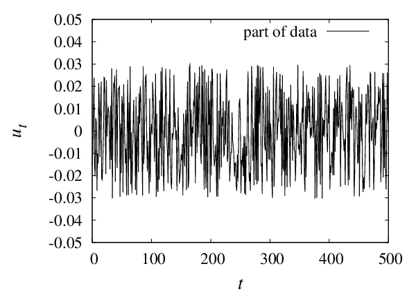
Figure 5 shows a part of the generated sequence by FFM with threshold. The amplitudes of high frequency random modes are larger than those in the sequence by FFM without threshold. So the sequence looks random at a glance, by comparing Fig. 1.
The effects of short-range randomness become obvious in the power spectrum. Figure 6 shows the power spectrum of the sequence generated by FFM with threshold. The spectrum is almost flat. The short-range random noises dominate the spectrum and prevent us to detect the long-range correlation.
The exponent is obtained as , if you apply the least square method for fitting all data points for the spectrum. The exponent obtained as is smaller than the expected value, by applying the fitting for long-range data points limited for . The power-spectrum analysis, namely, is strongly affected by short-range noises. It seems to be difficult to detect long-range correlations by analyzing the power spectrum.

The DFA analysis is more useful in this case than power-spectrum analyses. Figure 7 shows the result of the DFA analysis. It shows crossover of two regions. The exponent is for the shorter region. It is the value for random sequences. And for the longer region it is , which corresponds to the expected correlation. The crossover point of these two regions locates at the threshold . The DFA analysis, namely, detects the existence of long-range correlation and gives the threshold , above which random noises dominate.

IV Coarse-grained Sequence
Real observed data, in general, will contain various types of irregularity in short-range area. The simplest practical way to eliminate such irregularity is to sum data over some short length. We examine that this simple method preserves the long-range correlation in the original sequence as you expect.
The sequence generated in the previous section contains short-range random noises with long-range correlations. The DFA analysis gives the threshold , at which short-range noises dominate. Summing data over segments of length will eliminate those noises. Figure 8 shows the coarse-grained data obtained by summation up to . It shows the existence of long-range correlations.


Figure 9 shows the power spectrum of the coarse-grained sequence. Fitting all data by the least square method gives the exponent , which is slightly different from the imposed one .
The DFA analysis for the coarse-grained sequence gives the exponent as shown in Fig. 10. The power-law correlation with installed into the sequence is recovered and is detected by the DFA method.

V Summary and Discussion
Power-law correlations contained in temporal data of various dynamical systems have attracted research interests in various research fields. Increment of the amount of data sometimes means improvement of temporal resolution. Improvement of temporal resolution of data sometimes introduces asynchronous irregularity into data. Those short-range noises may prevent us from analyzing long-term correlations.
Short-range noises is shown to affect strongly the power-spectrum analysis. It is very difficult to detect long-range correlation, if the data contain such short-range noises.
The detrended fluctuation analysis (DFA) can detect both the short-range noises and the long-range correlations. There two ranges intersect at a threshold. The DFA also gives the threshold dividing these two ranges.
Finally we discuss the practicality of this work. A e-mail service is one of the most popular services in the Internet. Users send e-mail messages to e-mail servers of their own organization or those operated by Internet service providers. E-mail servers record e-mail sending requests usually every second. Every record contains the sender and receiver addresses and the message size. Namely the amount of sent messages is recorded every second.

A user will send his message to another user. The receiver will respond the message by quoting the received message after some delay. Therefore the sequence of the amount of e-mail messages will contain long-range correlations.
Figure 11 shows the result of the DFA analysis for the amount of e-mail messages at a e-mail server. In the shorter range than one hour, the exponent is , which corresponds to one for random noises. In the longer range than one hour, the long range correlation with can be found.
The number of the data points of this observation is of order . The short range to the order is dominated random noises. Namely the study in this paper with artificial sequences will be applicable to real observed data. The detail analysis of the cases for e-mail messages will be discussed elsewhere.
Acknowledgements.
The author would like to thank Y. Hieida and Y. Matsubara for their stimulating discussion. A part of this work is financially supported by a Grant-in-Aid for Scientific Research, No.18500215 and No.20360045, from the Ministry of Education, Culture, Sports, Science and Technology, Japan.References
- [1] C.-K. Peng, S. V. Buldyrev, S. Havlin, M. Simons, H. E. Stanley, and A. L. Goldberger, Phys. Rev. E 49, 1685 (1994).
- [2] C.-K. Peng, S. Havlin, H. E. Stanley, and A. L. Goldberger, Chaos 5, 82 (1995).
- [3] V. Paxson and V. Floyd, IEEE/ACM Trans. Networking 3, 226 (1995).
- [4] S.-i. Tadaki, J. Phys. Soc. Japan 76, 044001 (2007).
- [5] I. Csabai, J. Phys. A: Math. Gen. 27, L417 (1994).
- [6] M. Takayasu, H. Takayasu, and T. Sato, Physica A 233, 824 (1996).
- [7] T. Oetiker, MRTG - Tobi Oetiker’s MRTG - The Multi Router Traffic Grapher, http://oss.oetiker.ch/mrtg/.
- [8] V. J. Ribeiro, Z.-L. Zhang, S. Moon, and C. Diot, Computer Networks 48, 315 (2005).
- [9] C.-K. Peng, S. Havlin, M. Schwartz, and H. E. Stanley, Phys. Rev. A 44, R2239 (1991).
- [10] S. Prakash, S. Havlin, M. Schwartz, and H. E. Stanley, Phys. Rev. A 46, R1724 (1992).
- [11] H. A. Makse, S. Havlin, M. Schwartz, and H. E. Stanley, Phys. Rev. E 53, 5445 (1996).