Corrections to LRT on Large Dimensional Covariance Matrix by RMT^??

Zhidong Bai^?? Dandan Jiang Jian-feng Yao Shurong Zheng

Abstract

In this paper, we give an explanation to the failure of two likelihood ratio procedures for testing about covariance matrices from Gaussian populations when the dimension is large compared to the sample size. Next, using recent central limit theorems for linear spectral statistics of sample covariance matrices and of random F-matrices, we propose necessary corrections for these LR tests to cope with high-dimensional effects. The asymptotic distributions of these corrected tests under the null are given. Simulations demonstrate that the corrected LR tests yield a realized size close to nominal level for both moderate $p$ (around 20) and high dimension, while the traditional LR tests with $\chi^{2}$ approximation fails.

Another contribution from the paper is that for testing the equality between two covariance matrices, the proposed correction applies equally for non-Gaussian populations yielding a valid pseudo-likelihood ratio test.

keywords

[class=AMS] Primary 62H15 ; secondary 62H10

keywords

High-dimensional data , Testing on covariance matrices , Marčenko-Pastrur distributions , Random F-matrices

and and and

Zhidong Bai, Dandan Jiang and Shurong Zheng
KLASMOE and School of Mathematics and Statistics
Northeast Normal University
5268 People’s Road
130024 Changchun, China
and
Department of Statistics and Applied Probability
National University of Singapore
10, Kent Ridge Crescent
Singapore 119260
??, ??, ??

Jian-feng Yao
IRMAR and Université de Rennes 1
Campus de Beaulieu
35042 Rennes Cedex, France
??

1 Introduction

The rapid development and wide application of computer techniques permits to collect and store a huge amount data, where the number of measured variables is usually large. Such high dimensional data occur in many modern scientific fields, such as micro-array data in biology, stock market analysis in finance and wireless communication networks. Traditional estimation or test tools are no more valid, or perform badly for such high-dimensional data, since they typically assume a large sample size $n$ with respect to the number of variables $p$ . A better approach in this high-dimensional data setting would be based on asymptotic theory which has both $n$ and $p$ approaching infinity. To illustrate this purpose, let us mention the case of Hotelling’s $T^{2}$ -test. The failure of $T^{2}$ -test for high-dimensional data has been mentioned as early as by Dempster (1958). As a remedy, Dempster proposed a so-called non-exact test. However, the theoretical justification of Dempster’s test arises much later in Bai and Saranadasa (1996) inspired by modern random matrix theory (RMT). These authors have found necessary correction for the $T^{2}$ -test to compensate effects due to high dimension.

In this paper, we consider two LR tests concerning covariance matrices. We first give a theoretical explanation for the fail of these tests in high-dimensional data context. Next, with the aid of random matrix theory, we provide necessary corrections to these LR tests to cope with the high dimensional effects.

First, we consider the problem of one-sample covariance hypothesis test. Suppose that $\mathbf{x}$ follows a $p$ -dimensional Gaussian distribution $N(\mu_{p},\Sigma_{p})$ and we want to test

H_{0}:\penalty\ \Sigma_{p}=I_{p}\penalty\ ,

(1.1)

where $I_{p}$ denotes the $p$ -dimensional identity matrix. Note that testing $\Sigma_{p}=A$ with an arbitrary covariance matrix $A$ can always be reduced to the above null hypothesis by the transformation $A^{-\frac{1}{2}}\mathbf{x}$ .

Let $(\textbf{x}_{1},\cdots,\textbf{x}_{n})$ be a sample from $\mathbf{x}$ , where we assume $p<n$ . The sample covariance matrix is

\textbf{S}=\frac{1}{n}\sum\limits_{i=1}^{p}(\textbf{x}_{i}-\overline{\textbf{x}})(\textbf{x}_{i}-\overline{\textbf{x}})^{*},

(1.2)

and set

L^{*}=tr\textbf{S}-\log|\textbf{S}|-p\penalty\ .

(1.3)

The likelihood ratio test statistic is

T_{n}=n\cdot L^{*}.

(1.4)

Keeping $p$ fixed while letting $n\rightarrow\infty$ , then the classical theory depicts that $T_{n}$ converges to the $\chi^{2}_{\frac{1}{2}p(p+1)}$ distribution under $H_{0}$ .

However, as it will be shown, this classical approximation leads to a test size much higher than the nominal test level in the case of high-dimensional data, because $T_{n}$ approaches infinity for large $p$ . As seen from Table 1 in §3, for dimension and sample sizes $(p,n)=(50,500)$ , the realized size of the test is 22.5% instead of the nominal 5% level. The result is even worse for the case $(p,n)=(300,500)$ , with a 100% test size.

Based on a recent CLT for linear spectral statistics (LSS) of large-dimensional sample covariance matrices (Bai and Silverstein, 2004), we construct a corrected version of $T_{n}$ in §3. As shown by the simulation results of §3.1, the corrected test performs much better in case of high dimensions. Moreover, it also performs correctly for moderate dimensions like $p=10$ or 20. For dimension and sample sizes $(p,n)$ cited above, the sizes of the corrected test are 5.9% and 5.2%, respectively, both close to the 5% nominal level.

The second test problem we consider is about the equality between two high-dimensional covariance matrices. Let ${\bf x}_{i}=(x_{1i},x_{2i},\cdots,x_{pi})^{T},i=1,\cdots,n_{1}$ and ${\bf y}_{j}=(y_{1j},y_{2j},\cdots,y_{pj})^{T},$ $j=1,\cdots,n_{2}$ be observations from two $p$ -dimensional normal populations $N(\mu_{k},\Sigma_{k}),\penalty\ k=1,2$ , respectively. We wish to test the null hypothesis

H_{0}:\Sigma_{1}=\Sigma_{2}\penalty\ .

(1.5)

The related sample covariance matrices are

\displaystyle{A=\frac{1}{n_{1}}\sum\limits_{i=1}^{n_{1}}({\bf x}_{i}-\overline{{\bf x}})({\bf x}_{i}-\overline{{\bf x}})^{*},}\quad\displaystyle{B=\frac{1}{n_{2}}\sum\limits_{i=1}^{n_{2}}({\bf y}_{i}-\overline{{\bf y}})({\bf y}_{i}-\overline{{\bf y}})^{*},}

where $\overline{{\bf x}}$ , $\overline{{\bf y}}$ are the respective sample means. Let

L_{1}=\frac{\left|A\right|^{\frac{n_{1}}{2}}\cdot\left|B\right|^{\frac{n_{2}}{2}}}{\left|c_{1}A+c_{2}B\right|^{\frac{N}{2}}},

(1.6)

where $N=n_{1}+n_{2}$ and $c_{k}$ denote $\frac{n_{k}}{N},k=1,2.$ The likelihood ratio test statistic is

T_{N}=-2\log L_{1},

and when $n_{1},n_{2}\rightarrow\infty$ , we get

T_{N}=-2\log L_{1}\Rightarrow\chi^{2}_{\frac{1}{2}p(p+1)}

(1.7)

under $H_{0}$ . Of cause, in this limit scheme, the data dimension $p$ is held fixed.

However, employing this $\chi^{2}$ limit distribution for dimensions like 30 or 40, increases dramatically the size of the test. For instance, simulations in §4.1 show that, for dimension and sample sizes $(p,n_{1},n_{2})=(40,800,400)$ , the test size equals 21.2% instead of the nominal 5% level. The result is worse for the case of $(p,n_{1},n_{2})=(80,1600,800)$ , leading to a 49.5% test size. The reason for this fail of classical LR test is the following. Modern RMT indicates that when both dimension and sample size are large, the likelihood ratio statistic $T_{N}$ drifts to infinity almost surely. Therefore, the classical $\chi^{2}$ approximation leads to many false rejections of $H_{0}$ in case of high-dimensional data.

Based on recent CLT for linear spectral statistics of $F$ -matrices from RMT, we propose a correction to this LR test in §4. Although this corrected test is constructed under the asymptotic scheme $n_{1}\wedge n_{2}\rightarrow+\infty$ , $y_{n_{1}}={p}/{n_{1}}\rightarrow y_{1}\in(0,1)$ , $y_{n_{2}}={p}/{n_{2}}\rightarrow y_{2}\in(0,1)$ , simulations demonstrate an overall correct behavior including small or moderate dimensions $p$ . For example, for the above cited dimension and sample sizes $(p,n_{1},n_{2})$ , the sizes of the corrected test equal 5.6% and 5.2%, respectively, both close to the nominal 5% level.

Related works include Ledoit and Wolf (2002), Srivastava (2005) and Schott (2007). These authors propose several procedures in the high-dimensional setting for testing that i) a covariance matrix is an identity matrix, proportional to an identity matrix (spherecity) and is a diagonal matrix or ii) several covariance matrices are equal. These procedures have the following common feature: their construction involves some well-chosen distance function between the null and the alternative hypotheses and rely on the first two spectral moments, namely the statistics tr $S_{k}$ and tr $S_{k}^{2}$ from sample covariance matrices $S_{k}$ . Therefore, the procedures proposed by these authors are different from the likelihood-based procedures we consider here. Another important difference concerns the Gaussian assumption on the random variables used in all these references. Actually, for testing the equality between two covariance matrices, the correction proposed in this paper applies equally for non-Gaussian and high-dimensional data leading to a valid pseudo-likelihood test.

The rest of the paper is organized as following. Preliminary and useful RMT results are recalled in §2. In §3 and §4, we introduce our results for the two tests above. Proofs and technical derivations are postponed to the last section.

2 Useful results from the random matrix theory

We first recall several results from RMT, which will be useful for our corrections to tests. For any $p\times p$ square matrix $M$ with real eigenvalues $\left(\lambda_{i}^{M}\right)$ , $F_{n}^{M}$ denotes the empirical spectral distribution (ESD) of $M$ , that is,

F_{n}^{M}(x)=\frac{1}{p}\sum\limits_{i=1}^{p}\textbf{ 1}_{\lambda_{i}^{M}\leq x},\quad\quad x\in\mathbb{R}.

We will consider random matrix $M$ whose ESD $F_{n}^{M}$ converges (in a sense to be precised ) to a limiting spectral distribution (LSD) $F^{M}$ . To make statistical inference about a parameter $\theta=\int f(x)dF^{M}(x)$ , it is natural to use the estimator

\widehat{\theta}=\int f(x)dF_{n}^{M}(x)=\frac{1}{p}\sum\limits_{i=1}^{p}f(\lambda_{i}^{M}),

which is a so-called linear spectral statistic (LSS) of the random matrix $M$ .

2.1 CLT for LSS of a high-dimensional sample covariance matrix

Let $\{\xi_{ki}\in\mathbb{C},i,k=1,2,\cdots\}$ be a double array of $i.i.d.$ complex variables with mean 0 and variance 1. Set $\xi_{i}=(\xi_{1i},\xi_{2i},\cdots,\xi_{pi})^{T}$ , the vectors $(\xi_{1},\cdots,\xi_{n})$ is considered as an $i.i.d$ sample from some $p$ -dimensional distribution with mean $0_{p}$ and covariance matrix $I_{p}$ . Therefore the sample covariance matrix is

S_{n}={1\over{n}}\sum\limits_{i=1}^{n}\xi_{i}\xi_{i}^{*}.

(2.1)

For $0<\theta\leq 1$ , let $a(\theta)=(1-\sqrt{\theta})^{2}$ and $b(\theta)=(1+\sqrt{\theta})^{2}$ . The Marčenko-Pastur distribution of index $\theta$ , denoted as $F^{\theta}$ , is the distribution on $[a(\theta),b(\theta)]$ with the following density function

g_{\theta}(x)=\frac{1}{2\pi\theta x}\sqrt{[b(\theta)-x][x-a(\theta)]},\quad a(\theta)\leq x\leq b(\theta).

Let

y_{n}=\frac{p}{n}\rightarrow y\in(0,1)

and $F^{y},F^{y_{n}}$ be the Marčenko-Pastur law of index $y\penalty\ \mbox{and}\penalty\ y_{n}$ , respectively. Let $\mathcal{U}$ be an open set of the complex plane, including $[I_{(0,1)}(y)a(y),b(y)]$ , and $\mathcal{A}$ be the set of analytic functions $f:\mathcal{U}\mapsto\mathbb{C}.$ We consider the empirical process $G_{n}:=\{G_{n}(f)\}$ indexed by $\mathcal{A}$ ,

G_{n}(f)=p\cdot\int_{-\infty}^{+\infty}f(x)\left[F_{n}-F^{y_{n}}\right](dx),\penalty\ \penalty\ \penalty\ \penalty\ \penalty\ \penalty\ \quad f\in\mathcal{A},

(2.2)

where $F_{n}$ is the ESD of $S_{n}$ . The following theorem will play a fundamental role in next derivations, which is a specialization of a general theorem from Bai and Silverstein (2004) (Theorem 1.1).

Theorem 2.1.

Assume that $f_{1},\cdots,f_{k}\in\mathcal{A}$ , and $\{\xi_{ij}\}$ are $i.i.d.$ random variables, such that $E\xi_{11}=0,\penalty\ E{|\xi_{11}|^{2}}=1,\penalty\ E{|\xi_{11}|}^{4}<\infty.$ Moreover, $\frac{p}{n}\rightarrow y\in(0,1)$ as $n,p\rightarrow\infty.$
Then:
(i) Real Case. Assume $\{\xi_{ij}\}$ are real and $E(\xi_{11}^{4})=3.$ Then the random vector $\left(G_{n}(f_{1}),\cdots,G_{n}(f_{k})\right)$ weakly converges to a $k$ -dimensional Gaussian vector with mean vector,

m(f_{j})=\frac{f_{j}\left(a(y)\right)+f_{j}\left(b(y)\right)}{4}-\frac{1}{2\pi}\int_{a(y)}^{b(y)}\frac{f_{j}(x)}{\sqrt{4y-(x-1-y)^{2}}}dx,\quad j=1,\cdots,k,

(2.3)

and covariance function

\upsilon\left(f_{j},f_{\ell}\right)=-\frac{1}{2\pi^{2}}\oint\oint\frac{f_{j}(z_{1})f_{\ell}(z_{2})}{(\underline{m}(z_{1})-\underline{m}(z_{2}))^{2}}d\underline{m}(z_{1})d\underline{m}(z_{2}),\quad j,\ell\in\{1,\cdots,k\}\quad

(2.4)

where $\underline{m}(z)\equiv m_{\underline{F}^{y}}(z)$ is the Stieltjes Transform of $\underline{F}^{y}\equiv(1-y)I_{[0,\infty)}+yF^{y}$ . The contours in (2.4) are non overlapping and both contain the support of $F^{y}$ .

(ii) Complex Case. Assume $\{\xi_{ij}\}$ are complex and $E\xi^{2}_{11}=0$ , $E(|\xi_{11}|^{4})=2$ . Then the conclusion of (i) also holds, except the mean vector is zero and the covariance function is half of the function given in (2.4).

It is worth noticing that Theorem 1.1 in Bai and Silverstein (2004) covers more general sample covariance matrices of form $S^{\prime}_{n}=T_{n}^{1/2}S_{n}T_{n}^{1/2}$ where $(T_{n})$ is a given sequence of positive-definite Hermitian matrices. In the “white” case $T_{n}\equiv I$ as considered here, in a recent preprint Pastur and Lytova (2008), the authors offer a new extension of the CLT where the constraints $E|\xi_{11}|^{4}=3$ or 2, as stated above, are removed.

2.2 CLT for LSS of high-dimensional F matrix

Let $\{\xi_{ki}\in\mathbb{C},i,k=1,2,\cdots\}$ and $\{\eta_{kj}\in\mathbb{C},j,k=1,2,\cdots\}$ are two independent double arrays of $i.i.d.$ complex variables with mean 0 and variance 1. Write $\xi_{i}=(\xi_{1i},\xi_{2i},\cdots,\xi_{pi})^{T}$ and $\eta_{j}=(\eta_{1j},\eta_{2j},\cdots,\eta_{pj})^{T}$ . Also, for any positive integers $n_{1},n_{2}$ , the vectors $(\xi_{1},\cdots,\xi_{n_{1}})$ and $(\eta_{1},\cdots,\eta_{n_{2}})$ can be thought as independent samples of size $n_{1}$ and $n_{2}$ , respectively, from some $p$ -dimensional distributions. Let $S_{1}$ and $S_{2}$ be the associated sample covariance matrices, $i.e.$

S_{1}={1\over{n_{1}}}\sum\limits_{i=1}^{n_{1}}\xi_{i}\xi_{i}^{*}\quad\mbox{and}\quad S_{2}={1\over{n_{2}}}\sum\limits_{j=1}^{n_{2}}\eta_{j}\eta_{j}^{*}

Then, the following so-called F-matrix generalizes the classical Fisher-statistics for the present $p$ -dimensional case,

V_{n}=S_{1}S_{2}^{-1}

(2.5)

where $n_{2}>p$ . Here we use the notation $n=(n_{1},n_{2})$ .

Let

y_{n_{1}}=\frac{p}{n_{1}}\rightarrow y_{1}\in(0,1),\penalty\ y_{n_{2}}=\frac{p}{n_{2}}\rightarrow y_{2}\in(0,1).

(2.6)

Under suitable moment conditions, the ESD $F_{n}^{V_{n}}$ of $V_{n}$ has a LSD $F_{y_{1},y_{2}}$ , which has a density [See P72 of Bai and Silverstein (2006)], given by

\displaystyle{\ell(x)}=\left\{\begin{array}[]{ll}&\displaystyle{\frac{(1-y_{2})\sqrt{(b-x)(x-a)}}{2\pi x(y_{1}+y_{2}x)},\quad\penalty\ a\leq x\leq b,}\\[17.07164pt] &\displaystyle{0,\quad\quad\quad\quad\mbox{otherwise}.}\end{array}\right.

(2.7)

where $a=(1-y_{2})^{-2}\left(1-\sqrt{y_{1}+y_{2}-y_{1}y_{2}}\right)^{2}\penalty\ \mbox{and}\penalty\ b=(1-y_{2})^{-2}\left(1+\sqrt{y_{1}+y_{2}-y_{1}y_{2}}\right)^{2}.$

Similar to previously, let $\widetilde{\mathcal{U}}$ be an open set of the complex plane, including the interval

\left[I_{(0,1)}(y_{1})\frac{(1-\sqrt{y_{1}})^{2}}{(1+\sqrt{y_{2}})^{2}},\quad\frac{(1+\sqrt{y_{1}})^{2}}{(1-\sqrt{y_{2}})^{2}}\right],

and $\widetilde{\mathcal{A}}$ be the set of analytic functions $f:\widetilde{\mathcal{U}}\mapsto\mathbb{C}.$ Define the empirical process $\widetilde{G_{n}}:=\{\widetilde{G_{n}}(f)\}$ indexed by $\widetilde{\mathcal{A}}$

\widetilde{G_{n}}(f)=p\cdot\int_{-\infty}^{+\infty}f(x)\left[F_{n}^{V_{n}}-F_{y_{n_{1}},y_{n_{2}}}\right](dx),\penalty\ \penalty\ \penalty\ \penalty\ \penalty\ \penalty\ f\in\widetilde{\mathcal{A}}.

(2.8)

Here $F_{y_{n_{1}},y_{n_{2}}}$ is the limiting distribution in (2.7) but with $y_{n_{k}}$ instead of $y_{k},k=1,2.$

Recently, Zheng (2008) establishes a general CLT for LSS of large-dimensional F matrix. The following theorem is a simplified one quoted from it, which will play an important role.

Theorem 2.2.

Let $f_{1},\cdots,f_{k}\in\widetilde{\mathcal{A}}$ , and assume:
For each p, $(\xi_{ij_{1}})$ and $(\eta_{ij_{2}})$ variables are $i.i.d.$ , $1\leq i\leq p,\penalty\ 1\leq j_{1}\leq n_{1},\penalty\ 1\leq j_{2}\leq n_{2}.$ $E\xi_{11}=E\eta_{11}=0,$ $E|\xi_{11}|^{4}=E|\eta_{11}|^{4}<\infty,$ $y_{n_{1}}=\frac{p}{n_{1}}\rightarrow y_{1}\in(0,1),\quad y_{n_{2}}=\frac{p}{n_{2}}\rightarrow y_{2}\in(0,1).$
Then
(i) Real Case. Assume $(\xi_{ij})$ and $(\eta_{ij})$ are real, $E|\xi_{11}|^{2}=E|\eta_{11}|^{2}=1$ , then the random vector $\left(\widetilde{G_{n}}(f_{1}),\cdots,\widetilde{G_{n}}(f_{k})\right)$ weakly converges to a k-dimensional Gaussian vector with the mean vector

$\displaystyle m(f_{j})$	$\displaystyle=$	$\displaystyle\lim\limits_{r\rightarrow 1_{+}}\left[(\ref{E1})+(\ref{E1betax})+(\ref{E1betay})\right]$	(2.9)
		$\displaystyle\quad\frac{1}{4\pi i}\oint_{\|\zeta\|=1}f_{j}(z(\zeta))\left[\frac{1}{\zeta-{1\over r}}+\frac{1}{\zeta+{1\over r}}-\frac{2}{\zeta+{y_{2}\over{hr}}}\right]d\zeta$	(2.9)
		$\displaystyle\quad+\frac{\beta\cdot y_{1}(1-y_{2})^{2}}{2\pi i\cdot h^{2}}\oint_{\|\zeta\|=1}f_{j}(z(\zeta))\frac{1}{(\zeta+\frac{y_{2}}{hr})^{3}}d\zeta$	(2.10)
		$\displaystyle\quad+\frac{\beta\cdot y_{2}(1-y_{2})}{2\pi i\cdot h}\oint_{\|\zeta\|=1}f_{j}(z(\zeta))\frac{\zeta+\frac{1}{hr}}{(\zeta+\frac{y_{2}}{hr})^{3}}d\zeta,\quad\quad j=1,\cdots,k,$	(2.11)

where $z(\zeta)=(1-y_{2})^{-2}\left[1+h^{2}+2h\mathcal{R}(\zeta)\right],\quad h=\sqrt{y_{1}+y_{2}-y_{1}y_{2}},$ $\beta=E|\xi_{11}|^{4}-3,$ and the covariance function as $1<r_{1}<r_{2}\downarrow 1$

$\displaystyle\upsilon(f_{j},f_{\ell})=\lim\limits_{1<r_{1}<r_{2}\rightarrow 1_{+}}\left[(\ref{cov1})+(\ref{cov1betax}))\right]$		(2.12)
	$\displaystyle-\displaystyle\frac{1}{2\pi^{2}}\oint_{\|\zeta_{2}\|=1}\oint_{\|\zeta_{1}\|=1}\frac{f_{j}(z(r_{1}\zeta_{1}))f_{\ell}(z(r_{2}\zeta_{2}))r_{1}r_{2}}{(r_{2}\zeta_{2}-r_{1}\zeta_{1})^{2}}d\zeta_{1}d\zeta_{2},$	(2.12)
	$\displaystyle-\frac{\beta\cdot(y_{1}+y_{2})(1-y_{2})^{2}}{4\pi^{2}h^{2}}\oint_{\|\zeta_{1}\|=1}\frac{f_{j}\left(z(\zeta_{1})\right)}{(\zeta_{1}+\frac{y_{2}}{hr_{1}})^{2}}d\zeta_{1}\oint_{\|\zeta_{2}\|=1}\frac{f_{\ell}\left(z(\zeta_{2})\right)}{(\zeta_{2}+\frac{y_{2}}{hr_{2}})^{2}}d\zeta_{2}$	(2.13)
	$\displaystyle j,\ell\in\{1,\cdots,k\}.$	(2.13)

(ii) Complex Case. Assume $(\xi_{ij})$ and $(\eta_{ij})$ are complex, $E(\xi_{11}^{2})=E(\eta_{11}^{2})=0,$ then the conclusion of (i) also holds, except the means are $\lim\limits_{r\rightarrow 1_{+}}\left[(\ref{E1betax})+(\ref{E1betay})\right]$ and the covariance function is $\lim\limits_{1<r_{1}<r_{2}\rightarrow 1_{+}}\left[\displaystyle\frac{1}{2}\cdot(\ref{cov1})+(\ref{cov1betax})\right],$ where $\beta=E|\xi_{11}|^{4}-2.\penalty\$

We should point out that Zheng’s CLT for $F$ -matrices covers more general situations then those cited in Theorem 2.2. In particular, the fourth-moments $E|\xi_{11}|^{4}$ and $E|\eta_{11}|^{4}$ can be different.

The following lemma will be used in §4 for an application of Theorem 2.2 to obtain the formula (4.5) and (4.6).

Lemma 2.1.

For the function $f(x)=\log(a+bx),\quad x\in\mathbb{R},\quad a,b>0$ , let $(c,d)$ be the unique solution to the equations

\left\{\begin{array}[]{llll}c^{2}+d^{2}=a(1-y_{2})^{2}+b(1+h^{2}),\\ cd=bh,\\ 0<d<c.\\ \end{array}\right.

Analogously, let $\gamma,\eta$ be the constants similar to $(c,d)$ but for the function $g(x)=\log(\alpha+\beta x),\quad\alpha>0,\quad\beta>0.$ Then, the mean and covariance functions in (2.9) and (2.12) equal to

	$\displaystyle m(f)$	$\displaystyle=$	$\displaystyle\frac{1}{2}\log\frac{(c^{2}-d^{2})h^{2}}{(ch-y_{2}d)^{2}},$
	$\displaystyle\upsilon(f,g)$	$\displaystyle=$	$\displaystyle 2bhd^{-1}c^{-1}\log{\frac{c\gamma}{c\gamma-d\eta}}.$

3 Testing the hypothesis that a high-dimensional covariance matrix is equal to a given matrix

To test the hypothesis $H_{0}:\penalty\ \Sigma_{p}=I_{p}$ , let be the sample covariance matrix S and likelihood ratio statistic $T_{n}$ as defined in (1.2) and (1.4), respectively. For $\xi_{i}=\textbf{x}_{i}-\mu_{p},$ the array $\{\xi_{i}\}_{i=1,\cdots,n}$ contains $p$ -dimensional standard normal variables under $H_{0}$ . Let

\textbf{S}_{n}={1\over{n}}\sum\limits_{i=1}^{n}\xi_{i}\xi_{i}^{*}.

and

\widetilde{L^{*}}=\mbox{tr}\textbf{S}_{n}-\log|\textbf{S}_{n}|-p.

Theorem 3.1.

Assuming that the conditions of Theorem 2.1 hold, $L^{*}$ is defined as (1.3) and $g(x)=x-\log x-1$ . Then, under $H_{0}$ and when $n\rightarrow\infty$

\widetilde{T_{n}}=\upsilon(g)^{-\frac{1}{2}}\left[L^{*}-p\cdot F^{y_{n}}(g)-m(g)\right]\Rightarrow N\left(0,1\right),

(3.1)

where $F^{y_{n}}$ is the Marčenko-Pastur law of index $y_{n}$ .

Proof.

Because the difference between S and $\textbf{S}_{n}$ is a rank-1 matrix, S and $\textbf{S}_{n}$ have the same LSD. So, $L^{*}$ and $\widetilde{L^{*}}$ have the same asymptotic distribution. We also have

$\displaystyle\widetilde{L^{*}}$	$\displaystyle=$	$\displaystyle\mbox{tr}\textbf{S}_{n}-\log\|\textbf{S}_{n}\|-p$
	$\displaystyle=$	$\displaystyle\sum\limits_{i=1}^{p}\left(\lambda_{i}^{\textbf{s}_{n}}-\log\lambda_{i}^{\textbf{s}_{n}}-1\right)=p\cdot\int(x-\log x-1)dF_{n}(x)$
	$\displaystyle=$	$\displaystyle p\cdot\int g(x)d\left(F_{n}(x)-F^{y_{n}}(x)\right)+p\cdot F^{y_{n}}(g),$

so that

G_{n}(g)=\widetilde{L^{*}}-p\cdot F^{y_{n}}(g).

(3.2)

By Theorem 2.1, $G_{n}(g)$ weakly converges to a Gaussian vector with the mean

m(g)=-\frac{\log{(1-y)}}{2}

(3.3)

and variance

\upsilon(g)=-2\displaystyle\log{(1-y)}-2y.

(3.4)

for the real case, which are calculated in §5. For the complex case, the mean $m(g)$ is zero and the variance is half of $\upsilon(g).$ Then, by (3.2) we arrive at

\widetilde{L^{*}}-p\cdot F^{y_{n}}(g)\penalty\ \Rightarrow\penalty\ N\left(m(g),\upsilon(g)\right),

(3.5)

where

F^{y_{n}}(g)=1-\frac{y_{n}-1}{y_{n}}\log{(1-y_{n})}

(3.6)

can be calculated by the density of LSD of sample covariance matrix in §5. Because $\widetilde{L^{*}}$ and $L^{*}$ have the same asymptotic distribution and (3.5), finally we get

\displaystyle\widetilde{T_{n}}=\upsilon(g)^{-\frac{1}{2}}\left[L^{*}-p\cdot F^{y_{n}}(g)-m(g)\right]\Rightarrow N\left(0,1\right).

∎

3.1 Simulation study I

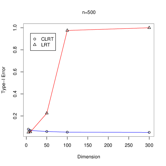
For different values of $(p,n)$ , we compute the realized sizes of traditional likelihood ratio test (LRT) and the corrected likelihood ratio test (CLRT) proposed previously. The nominal test level is set to be $\alpha=0.05$ , and for each $(p,n)$ , we run 10,000 independent replications with real Gaussian variables. Results are given in Table 1 and Figure 1 below.

	CLRT			LRT
(p, $n$ )	Size	Difference with 5%	Power	Size	Power
(5, 500)	0.0803	0.0303	0.6013	0.0521	0.5233
(10, 500)	0.0690	0.0190	0.9517	0.0555	0.9417
(50, 500)	0.0594	0.0094	1	0.2252	1
(100, 500)	0.0537	0.0037	1	0.9757	1
(300, 500)	0.0515	0.0015	1	1	1

Table 1: Sizes and powers of the traditional LRT and the corrected LRT, based on 10,000 independent applications with real Gaussian variables. Powers are estimated under the alternative

\Sigma_{p}=\mathop{\mathrm{diag}}(1,0.05,0.05,0.05,\ldots)

Refer to caption — Figure 1: Realized sizes of the traditional LRT and the corrected LRT for different dimensions $p$ with real Gaussian variables. 10 000 independent runs with 5% nominal level and sample size $n=500$ .

As seen from Table 1, the traditional LRT always rejects $H_{0}$ when $p$ is large, like $p=100$ or 300, while the sizes produced by the corrected LRT perfectly matches the nominal level. For moderate dimensions like $p=50$ , the corrected LRT still performs correctly while the traditional LRT has a size much higher than 5%.

4 Testing the equality of two high-dimensional covariance matrices

Let $({\bf x}_{i}),\penalty\ i=1,\cdots,n_{1}$ and $({\bf y}_{j}),\penalty\ j=1,\cdots,n_{2}$ be observations from two normal populations $N(\mu_{k},\Sigma_{k}),\penalty\ k=1,2$ , respectively. We examine the test defined in (1.5) and (1.6). The aim is to find a good scaling of the LR statistic $T_{N}$ , such that the scaled statistic weakly converges to some limiting distribution. Let

\xi_{i}=\Sigma^{-\frac{1}{2}}(\textbf{x}_{i}-\mu_{1}),\quad\eta_{i}=\Sigma^{-\frac{1}{2}}(\textbf{y}_{i}-\mu_{2})

where $\Sigma=\Sigma_{1}=\Sigma_{2}$ denotes the common covariance matrix under $H_{0}$ . Note that in a strict sense, the vectors $(\textbf{x}_{i}),(\textbf{y}_{i})$ and the matrices $\Sigma,\Sigma_{1},\Sigma_{2}$ depend on $p$ . However we do not signify this dependence in notations for ease of statements. Due to Gaussian assumption, the arrays $(\xi_{i})_{i=1,\cdots,n_{1}}$ and $(\eta_{j})_{j=1,\cdots,n_{2}}$ contain i.i.d. $N(0,1)$ variables, for which we can apply Theorem 2.2.

Let

	$\displaystyle S_{1}$	$\displaystyle=$	$\displaystyle{1\over{n_{1}}}\sum\limits_{i=1}^{n_{1}}\xi_{i}\xi_{i}^{*}=\Sigma^{-\frac{1}{2}}C\Sigma^{-\frac{1}{2}}$
	$\displaystyle S_{2}$	$\displaystyle=$	$\displaystyle{1\over{n_{2}}}\sum\limits_{j=1}^{n_{2}}\eta_{j}\eta_{j}^{*}=\Sigma^{-\frac{1}{2}}D\Sigma^{-\frac{1}{2}},$

where

	$\displaystyle C$	$\displaystyle=$	$\displaystyle\frac{1}{n_{1}}\sum\limits_{i=1}^{n_{1}}({\bf x}_{i}-\mu_{1})({\bf x}_{i}-\mu_{1})^{*},$
	$\displaystyle D$	$\displaystyle=$	$\displaystyle\frac{1}{n_{2}}\sum\limits_{j=1}^{n_{2}}({\bf y}_{j}-\mu_{2})({\bf y}_{j}-\mu_{2})^{*}.$

Note that

V_{n}=S_{1}S_{2}^{-1}

forms a random F-matrix and we have

\widetilde{L_{1}}=\frac{\left|S_{1}\right|^{\frac{n_{1}}{2}}\cdot\left|S_{2}\right|^{\frac{n_{2}}{2}}}{\left|c_{1}S_{1}+c_{2}S_{2}\right|^{\frac{N}{2}}}=\frac{\left|C\right|^{\frac{n_{1}}{2}}\cdot\left|D\right|^{\frac{n_{2}}{2}}}{\left|c_{1}C+c_{2}D\right|^{\frac{N}{2}}}.

(4.1)

Theorem 4.1.

Assuming that the conditions of Theorem 2.2 hold under $H_{0}$ , $L_{1}$ as defined in (1.6) and

f(x)=\log(y_{n_{1}}+y_{n_{2}}x)-\frac{y_{n_{2}}}{y_{n_{1}}+y_{n_{2}}}\log x-\log(y_{n_{1}}+y_{n_{2}}).

Then, under $H_{0}$ and as $n_{1}\wedge n_{2}\rightarrow\infty$ ,

\widetilde{T_{N}}=\upsilon(f)^{-\frac{1}{2}}\left[-\displaystyle\frac{2\log L_{1}}{N}-p\cdot F_{y_{n_{1}},y_{n_{2}}}(f)-m(f)\right]\Rightarrow N\left(0,1\right).

(4.2)

Proof.

As $A-C$ and $B-D$ are rank-1 random matrices, $AB^{-1}$ and $CD^{-1}$ have the same LSD. Also by (4.1), $\widetilde{L_{1}}$ and $L_{1}$ have the same asymptotic distribution. Because

$\displaystyle-\frac{2}{N}\log\widetilde{L_{1}}$	$\displaystyle=$	$\displaystyle-\frac{2}{N}\log\left(\frac{\left\|S_{1}\right\|^{\frac{n_{1}}{2}}\cdot\left\|S_{2}\right\|^{\frac{n_{2}}{2}}}{\left\|c_{1}S_{1}+c_{2}S_{2}\right\|^{\frac{N}{2}}}\right)$
	$\displaystyle=$	$\displaystyle\log{\|c_{1}V_{n}^{-1}+c_{2}\|}-c_{1}\cdot\log\|V_{n}^{-1}\|$
	$\displaystyle=$	$\displaystyle\sum\limits_{i=1}^{p}\log(c_{1}\lambda^{V_{n}}_{i}+c_{2})-c_{1}\cdot\log(\lambda^{V_{n}}_{i})$
	$\displaystyle=$	$\displaystyle p\cdot\int\left[\log(c_{1}x+c_{2})-c_{1}\cdot\log(x)\right]dF_{n}^{V_{n}}(x).$

Define $f(x)=\log(c_{1}x+c_{2})-c_{1}\cdot\log(x)$ , by $c_{1}=\frac{n_{1}}{N}=\frac{y_{n_{2}}}{y_{n_{1}}+y_{n_{2}}}$ and $c_{2}=\frac{n_{2}}{N}=\frac{y_{n_{1}}}{y_{n_{1}}+y_{n_{2}}}$ , also it can be written as

f(x)=\log(y_{n_{1}}+y_{n_{2}}x)-\frac{y_{n_{2}}}{y_{n_{1}}+y_{n_{2}}}\log x-\log(y_{n_{1}}+y_{n_{2}}).

(4.3)

From

	$\displaystyle-\frac{2\log\widetilde{L_{1}}}{N}$	$\displaystyle=$	$\displaystyle p\cdot\int f(x)dF_{n}^{V_{n}}(x)$
		$\displaystyle=$	$\displaystyle p\cdot\int f(x)d\left(F_{n}^{V_{n}}(x)-F_{y_{n_{1}},y_{n_{2}}}(x)\right)+p\cdot F_{y_{n_{1}},y_{n_{2}}}(f),$

we get

\widetilde{G_{n}}(f)=-\frac{2\log\widetilde{L_{1}}}{N}-p\cdot F_{y_{n_{1}},y_{n_{2}}}(f).

(4.4)

By Theorem 2.2, $\widetilde{G_{n}}(f)$ weakly converges to a Gaussian vector with mean

m(f)=\frac{1}{2}\left[\log\left(\frac{y_{1}+y_{2}-y_{1}y_{2}}{y_{1}+y_{2}}\right)-\frac{y_{1}}{y_{1}+y_{2}}\log(1-y_{2})-\frac{y_{2}}{y_{1}+y_{2}}\log(1-y_{1})\right]

(4.5)

and variance

\upsilon(f)=-\frac{2y_{2}^{2}}{(y_{1}+y_{2})^{2}}\log(1-y_{1})-\frac{2y_{1}^{2}}{(y_{1}+y_{2})^{2}}\log(1-y_{2})-2\log\frac{y_{1}+y_{2}}{y_{1}+y_{2}-y_{1}y_{2}}

(4.6)

for the real case, which are calculated by Lemma 2.1 in §5. For the complex case, the mean $m(f)$ is zero and the variance is half of $\upsilon(f)$ . In other words,

\displaystyle-\frac{2\log\widetilde{L_{1}}}{N}-p\cdot F_{y_{n_{1}},y_{n_{2}}}(f)

\displaystyle\Rightarrow

\displaystyle N\left(m(f),\upsilon(f)\right),

(4.7)

where

$\displaystyle\displaystyle{F_{y_{n_{1}},y_{n_{2}}}(f)}$	$\displaystyle=$	$\displaystyle\displaystyle{\frac{-(y_{n_{1}}+y_{n_{2}}-y_{n_{1}}y_{n_{2}})}{y_{n_{1}}y_{n_{2}}}\log{(y_{n_{1}}+y_{n_{2}}-y_{n_{1}}y_{n_{2}})}}$
	$\displaystyle+$	$\displaystyle\displaystyle{\frac{(y_{n_{1}}+y_{n_{2}}-y_{n_{1}}y_{n_{2}})}{y_{n_{1}}y_{n_{2}}}\log{(y_{n_{1}}+y_{n_{2}})}}+\displaystyle{\frac{y_{n_{1}}(1-y_{n_{2}})}{y_{n_{2}}(y_{n_{1}}+y_{n_{2}})}\log{(1-y_{n_{2}})}}$
	$\displaystyle+$	$\displaystyle\displaystyle{\frac{y_{n_{2}}(1-y_{n_{1}})}{y_{n_{1}}(y_{n_{1}}+y_{n_{2}})}\log{(1-y_{n_{1}})}},$

is derived by use of the density of $F_{y_{n_{1}},y_{n_{2}}}$ in §5. Because $\widetilde{L_{1}}$ and $L_{1}$ have the same asymptotic distribution and by (4.7), we get by letting $n_{1}\wedge n_{2}\rightarrow\infty$ ,

\widetilde{T_{N}}=\upsilon(f)^{-\frac{1}{2}}\left[-\displaystyle\frac{2\log L_{1}}{N}-p\cdot F_{y_{n_{1}},y_{n_{2}}}(f)-m(f)\right]\Rightarrow N\left(0,1\right).

∎

4.1 Simulation study II

For different values of $(p,n_{1},n_{2})$ , we compute the realized sizes of the traditional LRT and the corrected LRT with 10,000 independent replications. The nominal test level is $\alpha=0.05$ and we use real Gaussian variables. Results are summarized in Table 2 and Figure 2.

(y1, y2)=(0.05, 0.05)
	CLRT			LRT
(p, $n_{1}$ , $n_{2}$ )	Size	Difference with 5%	Power	Size	Power
(5, 100, 100)	0.0770	0.0270	1	0.0582	1
(10, 200, 200)	0.0680	0.0180	1	0.0684	1
(20, 400, 400)	0.0593	0.0093	1	0.0872	1
(40, 800, 800)	0.0526	0.0026	1	0.1339	1
(80, 1600, 1600)	0.0501	0.0001	1	0.2687	1
(160, 3200, 3200)	0.0491	-0.0009	1	0.6488	1
(320, 6400, 6400)	0.0447	-0.0053	0.9671	1	1

(y1, y2)=(0.05, 0.1)
	CLRT			LRT
(p, $n_{1}$ , $n_{2}$ )	Size	Difference with 5%	Power	Size	Power
(5, 100, 50)	0.0781	0.0281	0.9925	0.0640	0.9849
(10, 200, 100)	0.0617	0.0117	0.9847	0.0752	0.9904
(20, 400, 200)	0.0573	0.0073	0.9775	0.1104	0.9938
(40, 800, 400)	0.0561	0.0061	0.9765	0.2115	0.9975
(80, 1600, 800)	0.0521	0.0021	0.9702	0.4954	0.9998
(160, 3200, 1600)	0.0520	0.0020	0.9702	0.9433	1
(320, 6400, 3200)	0.0510	0.0010	1	0.9939	1

Table 2: Sizes and powers of the traditional LRT and the corrected LRT based on 10,000 independent replications using real Gaussian variables. Powers are estimated under the alternative

\Sigma_{1}\Sigma_{2}^{-1}=\mbox{ diag}(3,1,1,1,\cdots)

. Upper:

y_{1}=y_{2}=0.05

. Bottom:

y_{1}=0.05,\penalty\ y_{2}=0.1

As we can see, when the dimension $p$ increases, the traditional LRT leads to a dramatically high test size while the corrected LRT remains accurate. Furthermore, for moderate dimensions like $p=20$ or 40, the sizes of the traditional LRT are much higher than 5%, whereas the ones of corrected LRT are very close. By a closer look at the column showing the difference with 5%, we note that this difference rapidly decrease as $p$ increases for the corrected test. Figure 2 gives a vivid sight of these comparisons between the traditional LRT and the corrected LRT in term of test sizes.

4.2 A pseudo-likelihood test for high-dimensional non-Gaussian data

As said in Introduction, previous related works as Ledoit and Wolf (2002), Srivastava (2005) or Schott (2007) all assume Gaussian variables. In contrast, Theorem 4.1 applies for general distributions having a fourth moment. For these non Gaussian data, we consider the corrected LRT as generalized pseudo-likelihood ratio test (or Gaussian LRT).

Moreover, the methods proposed by these authors all rely on an appropriate normalization of the trace of squared difference between two sample covariances following the idea of Bai and Saranadasa (1996). We believe that their method would strongly depend on the normality assumption (which was supported by simulation results below). On the other hand, based on general understanding, the LRT contains much higher information from data and its poor performance observed up to now is just caused by its large bias when dimension is large. Thus, from the intuitive understanding, we are confined ourselves to modify the LRT.

Let us develop in more details an example. Assume that x follows a normalized $t$ -distribution with 5 degree of freedom, that is $\textbf{x}=\sqrt{\frac{3}{5}}t(5),$ x and y are i.i.d., hence $E\textbf{x}=E\textbf{y}=0,$ $E|\textbf{x}|^{2}=E|\textbf{y}|^{2}=1$ and $E|\textbf{x}|^{4}=E|\textbf{y}|^{4}=9.$ We still employ the result in Theorem 4.1 for the test of equality between two covariance matrices, where

	$\displaystyle m_{1}(f)=$	$\displaystyle\displaystyle{\frac{1}{2}\Big[\log\left(\frac{y_{1}+y_{2}-y_{1}y_{2}}{y_{1}+y_{2}}\right)-\frac{y_{1}}{y_{1}+y_{2}}\log(1-y_{2})-\frac{y_{2}}{y_{1}+y_{2}}\log(1-y_{1})}$			(4.8)
		$\displaystyle\quad\quad\quad\quad\quad\quad\quad\quad+\displaystyle{\frac{6y_{1}^{2}y_{2}}{(y_{1}+y_{2})^{2}}+\frac{6y_{1}y_{2}^{2}}{(y_{1}+y_{2})^{2}}\Big]}$			(4.8)

and

\upsilon_{1}(f)=-\frac{2y_{2}^{2}}{(y_{1}+y_{2})^{2}}\log(1-y_{1})-\frac{2y_{1}^{2}}{(y_{1}+y_{2})^{2}}\log(1-y_{2})-2\log\frac{y_{1}+y_{2}}{y_{1}+y_{2}-y_{1}y_{2}}

(4.9)

instead of $m(f)$ and $\upsilon(f)$ for real case, respectively. (4.8) and (4.9) are calculated in §5.

The following Table 3 summarizes a simulation study where we compare this corrected pseudo-LRT with the test proposed in Schott (2007). We use 1,000 independent replications with the above $t$ -distributed variables. Again, the nominal test level is $\alpha=0.05$ . As we can see, the corrected pseudo-LRT performs correctly while Schott’s test is no more valid here since the variables are not Gaussian.

(y1, y2)=(0.05, 0.1)
(p, $n_{1}$ , $n_{2}$ )	CLRT Size	Schott’s Size
(10,100, 200)	0.067	0.517
(20, 200, 400)	0.065	0.603
(40, 400, 800)	0.054	0.703
(80, 800, 1600)	0.048	0.764
(160, 1600, 3200)	0.045	0.826
(320, 3200, 6400)	0.051	0.854

Table 3: Sizes of the corrected pseudo-likelihood ration test and Schott’s test for the case of

y_{1}=0.1,\penalty\ y_{2}=0.05

, based on 1,000 independent replications with normalized

t

-distributed variables with 5 degrees of freedom.

5 Proofs

Proof of (3.3)

By Theorem 2.1, for $g(x)=x-\log x-1$ , by using the variable change $x=1+y-2\sqrt{y}\cos\theta,\penalty\ 0\leq\theta\leq\pi$ , we have

$\displaystyle m(g)$	$\displaystyle=$	$\displaystyle\frac{g\left(a(y)\right)+g\left(b(y)\right)}{4}-\frac{1}{2\pi}\int_{a(y)}^{b(y)}\frac{g(x)}{\sqrt{4y-(x-1-y)^{2}}}dx$
	$\displaystyle=$	$\displaystyle\frac{y-\log(1-y)}{2}-\frac{1}{2\pi}\int_{0}^{\pi}\left[1+y-2\sqrt{y}\cos\theta-\log(1+y-2\sqrt{y}\cos\theta)-1\right]d\theta$
	$\displaystyle=$	$\displaystyle\frac{y-\log(1-y)}{2}-\frac{1}{4\pi}\int_{0}^{2\pi}\left[y-2\sqrt{y}\cos\theta-\log\|1-\sqrt{y}e^{i\theta}\|^{2}\right]d\theta$
	$\displaystyle=$	$\displaystyle-\frac{\log(1-y)}{2},$

where $\displaystyle\int_{0}^{2\pi}\log|1-\sqrt{y}e^{i\theta}|^{2}d\theta=0$ is calculated in Bai and Silverstein (2004).

Proof of (3.4)

For $g(x)=x-\log x-1$ , by Theorem 2.1, we have

\upsilon(g)=-\frac{1}{2\pi^{2}}\oint\oint\frac{g(z_{1})g(z_{2})}{(\underline{m}(z_{1})-\underline{m}(z_{2}))^{2}}d\underline{m}(z_{1})d\underline{m}(z_{2})

and

	$\displaystyle g(z_{1})g(z_{2})$	$\displaystyle=$	$\displaystyle z_{1}z_{2}-z_{1}\log z_{2}-z_{2}\log z_{1}+\log z_{1}\log z_{2}$
			$\displaystyle-z_{1}+\log z_{1}-z_{2}+\log z_{2}+1.$

It is easy to see that $\upsilon(\textbf{1},\textbf{1})=0$ , where 1 means constant function equals to 1. For Stieltjes transform of $F^{y}$ , the following equation is given in Bai and Silverstein (2004), for $z\in\mathbb{C}^{+}$ ,

z=-\frac{1}{\underline{m}(z)}+\frac{y}{1+\underline{m}(z)}.

(5.1)

Let $m_{i}=\underline{m}(z_{i}),\penalty\ \penalty\ i=1,2$ . For fixed $m_{2}$ , we have on a contour enclosed 1, $(y-1)^{-1}$ and -1, but not 0,

$\displaystyle\displaystyle{\oint\frac{\log\left(z(m_{1})\right)}{(m_{1}-m_{2})^{2}}dm_{1}}$	$\displaystyle=$	$\displaystyle\displaystyle{\oint\frac{\frac{1}{m_{1}^{2}}-\frac{y}{(1+m_{1})^{2}}}{-\frac{1}{m_{1}}+\frac{y}{1+m_{1}}}\frac{1}{(m_{1}-m_{2})}dm_{1}}$
	$\displaystyle=$	$\displaystyle\displaystyle{\oint\frac{(1+m_{1})^{2}-ym_{1}^{2}}{ym_{1}(m_{1}-m_{2})}\left(\frac{-1}{m_{1}+1}+\frac{1}{m_{1}-\frac{1}{y-1}}\right)dm_{1}}$
	$\displaystyle=$	$\displaystyle\displaystyle{2\pi i\cdot\left(\frac{1}{m_{2}+1}-\frac{1}{m_{2}-\frac{1}{y-1}}\right)}.$

and

			$\displaystyle\displaystyle{\oint\frac{-\frac{1}{m_{1}}+\frac{y}{1+m_{1}}}{(m_{1}-m_{2})^{2}}dm_{1}}$
		$\displaystyle=$	$\displaystyle\displaystyle{y\oint(\frac{1}{1+m_{1}}+\frac{1-y}{y})\cdot[1-(1+m_{1})]^{-1}\cdot(m_{2}+1)^{-2}\cdot(1-\frac{m_{1}+1}{m_{2}+1})^{-2}dm_{1}}$
		$\displaystyle=$	$\displaystyle\displaystyle{y\oint(\frac{1}{1+m_{1}}+\frac{1-y}{y})\cdot\sum\limits^{\infty}_{j=0}(1+m_{1})^{j}(m_{2}+1)^{-2}\sum\limits^{\infty}_{\ell=1}\ell(\frac{m_{1}+1}{m_{2}+1})^{\ell-1}dm_{1}}$
		$\displaystyle=$	$\displaystyle\displaystyle{2\pi i\cdot\frac{y}{(m_{2}+1)^{2}}}.$

Then we also get $\upsilon(-z_{1}+\log z_{1},\penalty\ \textbf{1})=0$ . Similarly, $\upsilon(\textbf{1},\penalty\ -z_{2}+\log z_{2})=0$ . Furthermore,

\displaystyle\upsilon(z_{1},z_{2})

\displaystyle=

\displaystyle\displaystyle{\frac{y^{2}}{\pi i}\oint\frac{1}{(m_{2}+1)^{2}}(\displaystyle\frac{1}{1+m_{2}}+\displaystyle\frac{1-y}{y})\displaystyle\sum\limits^{\infty}_{j=0}(1+m_{2})^{j}dm_{2}}=2y,

and

$\displaystyle\upsilon(z_{1},\log z_{2})$	$\displaystyle=$	$\displaystyle\displaystyle{\frac{y}{\pi i}\oint(\frac{1}{m_{2}+1}-\frac{1}{m_{2}-1/(y-1)})(\frac{1}{1+m_{2}}+\frac{1-y}{y})\cdot[1-(1+m_{2})]^{-1}dm_{2}}$
	$\displaystyle=$	$\displaystyle\displaystyle{\frac{y}{\pi i}\oint(\frac{1}{m_{2}+1}-\frac{1}{m_{2}-1/(y-1)})(\frac{1}{1+m_{2}}+\displaystyle\frac{1-y}{y})\sum\limits^{\infty}_{j=0}(1+m_{2})^{j}dm_{2}}$
	$\displaystyle=$	$\displaystyle 2y.$

By a computation in Bai and Silverstein (2004), we know that $\upsilon(\log z_{1},\log z_{2})=-2\log(1-y)$ . Finally, we obtain

$\displaystyle\upsilon(g)$	$\displaystyle=$	$\displaystyle\upsilon(z_{1},z_{2})+\upsilon(\log z_{1},\log z_{2})-2\upsilon(z_{1},\log z_{2})$
		$\displaystyle\quad+\upsilon(-z_{1}+\log z_{1},\textbf{1})+\upsilon(\textbf{1},-z_{2}+\log z_{2})+\upsilon(\textbf{1},\textbf{1})$
	$\displaystyle=$	$\displaystyle-2\log(1-y)-2y.$

Proof of (3.6)

Since $F^{y_{n}}$ is the Marčenko-Pastur law of index $y_{n}$ , by using the variable change $x=1+y_{n}-2\sqrt{y_{n}}\cos\theta,\penalty\ 0\leq\theta\leq\pi$ we have

$\displaystyle F^{y_{n}}(g)$	$\displaystyle=$	$\displaystyle\int^{b(y_{n})}_{a(y_{n})}\frac{x-\log x-1}{2\pi xy_{n}}\sqrt{(b(y_{n})-x)(x-a(y_{n}))}dx$
	$\displaystyle=$	$\displaystyle\frac{1}{2\pi y_{n}}\int_{0}^{\pi}\left[1-\frac{\log(1+y_{n}-2\sqrt{y_{n}}\cos\theta)+1}{1+y_{n}-2\sqrt{y_{n}}\cos\theta}\right]4y_{n}\sin^{2}\theta d\theta$
	$\displaystyle=$	$\displaystyle\frac{1}{2\pi}\int_{0}^{2\pi}\left[2\sin^{2}\theta-\frac{2\sin^{2}\theta}{1+y_{n}-2\sqrt{y_{n}}\cos\theta}\left(\log\|1-\sqrt{y_{n}}e^{i\theta}\|^{2}-1\right)\right]d\theta$
	$\displaystyle=$	$\displaystyle 1-\frac{y_{n}-1}{y_{n}}\log(1-y_{n}),$

where

\displaystyle{\frac{1}{2\pi}\int_{0}^{2\pi}\frac{2\sin^{2}\theta}{1+y_{n}-2\sqrt{y_{n}}\cos\theta}\log|1-\sqrt{y_{n}}e^{i\theta}|^{2}d\theta}=\displaystyle{\frac{y_{n}-1}{y_{n}}\log(1-y_{n})-1}

is calculated in Bai and Silverstein (2004).

Proof of Lemma 2.1

We use the variable change $x=(1-y_{2})^{-2}(1+h^{2}-2h\cos\theta)$ , where $h=\sqrt{y_{1}+y_{2}-y_{1}y_{2}}$ . When $c,d$ satisfy $c^{2}+d^{2}=a(1-y_{2})^{2}+b(1+h^{2}),\penalty\ cd=bh,\penalty\ 0<d<c,$ we have

f(z(\xi))=\log(a+bz(\xi))=\log\left(\frac{\left|c+d\xi\right|^{2}}{(1-y_{2})^{2}}\right).

Similarly,

g(z(\xi))=\log(\alpha+\beta z(\xi))=\log\left(\frac{\left|\gamma+\eta\xi\right|^{2}}{(1-y_{2})^{2}}\right).

Let

\widetilde{f}(z(\xi))=\log\left(\frac{\left(c+d\xi\right)^{2}}{(1-y_{2})^{2}}\right)\quad\mbox{and}\quad\widetilde{g}(z(\xi))=\log\left(\frac{\left(\gamma+\eta\xi\right)^{2}}{(1-y_{2})^{2}}\right).

Note that $f(z(\xi))=\Re(\widetilde{f}(z(\xi)))\quad\mbox{and}\quad g(z(\xi))=\Re(\widetilde{g}(z(\xi)))$ . By Theorem 2.2, we have

$\displaystyle m(f)$	$\displaystyle=$	$\displaystyle\displaystyle{\frac{1}{4\pi i}\oint_{\|\xi\|=1}f(z(\xi))\left[\frac{1}{\xi-{1\over r}}+\frac{1}{\xi+{1\over r}}-\frac{2}{\xi+{y_{2}\over{hr}}}\right]d\xi}$
	$\displaystyle=$	$\displaystyle\displaystyle{\frac{1}{4\pi}\int^{2\pi}_{0}f(z(e^{i\theta}))\left[\frac{1}{e^{i\theta}-{1\over r}}+\frac{1}{e^{i\theta}+{1\over r}}-\frac{2}{e^{i\theta}+{y_{2}\over{hr}}}\right]e^{i\theta}d\theta}$
	$\displaystyle=$	$\displaystyle\displaystyle{\frac{1}{4\pi}\int^{2\pi}_{0}f(z(e^{i\theta}))\left[\frac{1}{e^{-i\theta}-{1\over r}}+\frac{1}{e^{-i\theta}+{1\over r}}-\frac{2}{e^{-i\theta}+{y_{2}\over{hr}}}\right]e^{-i\theta}d\theta}$
	$\displaystyle=$	$\displaystyle\displaystyle\frac{1}{8\pi}\int^{2\pi}_{0}f(z(e^{i\theta}))\Bigg\{\left[\frac{1}{e^{i\theta}-{1\over r}}+\frac{1}{e^{i\theta}+{1\over r}}-\frac{2}{e^{i\theta}+{y_{2}\over{hr}}}\right]e^{i\theta}+$
		$\displaystyle\left[\frac{1}{e^{-i\theta}-{1\over r}}+\frac{1}{e^{-i\theta}+{1\over r}}-\frac{2}{e^{-i\theta}+{y_{2}\over{hr}}}\right]e^{-i\theta}\Bigg\}d\theta$
	$\displaystyle=$	$\displaystyle\frac{1}{8\pi}\Re\Bigg\{\int^{2\pi}_{0}\widetilde{f}(z(e^{i\theta}))\Bigg[\left(\frac{1}{e^{i\theta}-{1\over r}}+\frac{1}{e^{i\theta}+{1\over r}}-\frac{2}{e^{i\theta}+{y_{2}\over{hr}}}\right)e^{i\theta}+$
		$\displaystyle\left(\frac{r}{r-e^{i\theta}}+\frac{r}{r+e^{i\theta}}-\frac{2hr}{y_{2}e^{i\theta}+hr}\right)\Bigg]d\theta\Bigg\}$
	$\displaystyle=$	$\displaystyle\Re\Bigg\{\frac{1}{8\pi i}\oint_{\|\xi\|=1}\widetilde{f}(z(\xi))\Bigg[\left(\frac{1}{\xi-{1\over r}}+\frac{1}{\xi+{1\over r}}-\frac{2}{\xi+{y_{2}\over{hr}}}\right)$
		$\displaystyle+\left(\frac{r}{r-\xi}+\frac{r}{r+\xi}-\frac{2hr}{y_{2}\xi+hr}\right)\xi^{-1}\Bigg]d\xi\Bigg\}$
	$\displaystyle=$	$\displaystyle\frac{1}{4}\left(\widetilde{f}(z(\frac{1}{r}))+\widetilde{f}(z(-\frac{1}{r}))-2\widetilde{f}(z(-\frac{y_{2}}{hr}))\right)$
	$\displaystyle\rightarrow$	${}^{r\downarrow 1}\frac{1}{4}\left[\widetilde{f}(z(1))+\widetilde{f}(z(-1))-2\widetilde{f}(z(-\frac{y_{2}}{h}))\right]$
	$\displaystyle=$	$\displaystyle\frac{1}{2}\log\frac{(c^{2}-d^{2})h^{2}}{(ch-y_{2}d)^{2}}.$

Let $m_{j}=-\frac{1+hr_{j}\xi_{j}}{1-y_{2}}$ , where $|\xi_{j}|=1,j=1,2,$ $r_{2}\downarrow r_{1},$ and $r_{1}\downarrow 1$ . By Theorem 2.2, we have

\upsilon(f,g)=-\frac{1}{2\pi^{2}}\oint_{|\xi_{2}|=1}\left\{\oint_{|\xi_{1}|=1}\frac{f(z(r_{1}\xi_{1}))}{(r_{2}\xi_{2}-r_{1}\xi_{1})^{2}}\cdot r_{1}r_{2}d\xi_{1}\right\}g(z(r_{2}\xi_{2}))d\xi_{2}.

When $r_{1}\downarrow 1,\quad-\frac{d}{cr_{1}}\quad\mbox{and}\quad 0$ are poles. We can then choose $r_{1}$ so that $-\frac{c}{dr_{1}}$ is a not a pole. Then we get

			$\displaystyle\displaystyle{\oint_{\|\xi_{1}\|=1}\frac{\log(a+bz(r_{1}\xi_{1}))}{(r_{2}\xi_{2}-r_{1}\xi_{1})^{2}}\cdot r_{1}r_{2}d\xi_{1}}$
		$\displaystyle=$	$\displaystyle\displaystyle{\oint_{\|\xi_{1}\|=1}\frac{\left(\log(a+bz(r_{1}\xi_{1}))\right)^{\prime}}{r_{1}\xi_{1}-r_{2}\xi_{2}}\cdot r_{2}d\xi_{1}}$
		$\displaystyle=$	$\displaystyle\displaystyle{\oint_{\|\xi_{1}\|=1}\Bigg[\frac{bhr_{1}\xi_{1}}{(r_{1}\xi_{1}-r_{2}\xi_{2})(c+dr_{1}\xi_{1})c}\cdot\frac{1}{\xi_{1}+\frac{d}{cr_{1}}}}$
			$\displaystyle\quad-\frac{bhr_{1}^{-1}}{(r_{1}\xi_{1}-r_{2}\xi_{2})(c+dr_{1}\xi_{1})c}\cdot\frac{1}{(\xi_{1}+\frac{d}{cr_{1}})\xi_{1}}\cdot r_{2}\Bigg]d\xi_{1}$
		$\displaystyle=$	$\displaystyle\displaystyle{2\pi i}\left(\frac{bhd^{-1}c^{-1}}{\xi_{2}}-\frac{bhd^{-1}r_{2}}{d+cr_{2}\xi_{2}}\right).$

So,

\upsilon(f,g)=-\frac{i}{\pi}\oint_{|\xi_{2}|=1}\left(\frac{bhd^{-1}c^{-1}}{\xi_{2}}-\frac{bhd^{-1}r_{2}}{d+cr_{2}\xi_{2}}\right)\log\left(\alpha+\beta z(r_{2}\xi_{2})\right)d\xi_{2}.

Since the function $g(x)=\log(\alpha+\beta x)$ is analytic, when $r_{2}>1$ but sufficiently close to 1, we have

\left|g(z(r\xi_{2}))-g(z(\xi_{2}))\right|\leq K(r-1),

for some constant $K$ . Thus we have

\begin{array}[]{lll}&\displaystyle{\left|\oint_{|\xi|_{2}=1}\left[g(z(r_{2}\xi_{2}))-g(z(\xi_{2}))\right]\left(\frac{bhd^{-1}c^{-1}}{\xi_{2}}-\frac{bhd^{-1}r_{2}}{d+cr_{2}\xi_{2}}\right)d\xi_{2}\right|}\\[11.38109pt] \rightarrow&0\quad\mbox{as}\quad r_{2}\downarrow 1,\end{array}

where the estimations are done according to $|\arg(\xi_{2})|$ or $|\arg(\xi_{2})-\pi|\leq\sqrt{r_{2}-1}$ or not. Thus,

\upsilon(f,g)=-\frac{i}{\pi}\oint_{|\xi_{2}|=1}g(z(\xi_{2}))\left(\frac{bhd^{-1}c^{-1}}{\xi_{2}}-\frac{bhd^{-1}r_{2}}{d+cr_{2}\xi_{2}}\right)d\xi_{2}+R(r_{2})

where $R(r_{2})\rightarrow 0,\quad\mbox{as}\quad r_{2}\downarrow 1.$ Because $\displaystyle{g(z(\xi_{2}))=\log\left(\frac{\left|\gamma+\eta\xi_{2}\right|^{2}}{(1-y_{2})^{2}}\right),}$ for $\gamma,\eta$ satisfying $\gamma^{2}+\eta^{2}=\alpha(1-y_{2})^{2}+\beta(1+h^{2}),\penalty\ \gamma\eta=\beta h,\penalty\ 0<\eta<\gamma,$ and if $\displaystyle{\widetilde{g}(z(\xi_{2}))=\log\left(\frac{\left(\gamma+\eta\xi_{2}\right)^{2}}{(1-y_{2})^{2}}\right),}$ we have $g(z(\xi_{2}))=\Re\left(\widetilde{g}(z(\xi_{2}))\right)$ . Therefore,

$\displaystyle\upsilon(f,g)=-\frac{i}{\pi}\oint_{\|\xi\|_{2}=1}g(z(\xi_{2}))\left(\frac{bhd^{-1}c^{-1}}{\xi_{2}}-\frac{bhd^{-1}r_{2}}{d+cr_{2}\xi_{2}}\right)d\xi_{2}$
	$\displaystyle=$	$\displaystyle\frac{1}{\pi}\int^{2\pi}_{0}g(z(e^{i\theta}))\left(\frac{bhd^{-1}c^{-1}}{e^{i\theta}}-\frac{bhd^{-1}r_{2}}{d+cr_{2}e^{i\theta}}\right)e^{i\theta}d\theta$
	$\displaystyle=$	${}^{\theta\rightarrow 2\pi-\theta}\penalty\ \penalty\ \frac{1}{\pi}\int^{2\pi}_{0}g(z(e^{i\theta}))\left(\frac{bhd^{-1}c^{-1}}{e^{-i\theta}}-\frac{bhd^{-1}r_{2}}{d+cr_{2}e^{-i\theta}}\right)e^{-i\theta}d\theta$
	$\displaystyle=$	$\displaystyle\frac{1}{2\pi}\int_{0}^{2\pi}g(z(e^{i\theta}))\Bigg[\left(\frac{bhd^{-1}c^{-1}}{e^{i\theta}}-\frac{bhd^{-1}r_{2}}{d+cr_{2}e^{i\theta}}\right)e^{i\theta}+bhd^{-1}c^{-1}-\frac{bhd^{-1}r_{2}}{de^{i\theta}+cr_{2}}\Bigg]d\theta$
	$\displaystyle=$	$\displaystyle\frac{1}{2\pi}\Re\Bigg\{\int_{0}^{2\pi}\widetilde{g}(z(e^{i\theta}))\Bigg[\left(\frac{bhd^{-1}c^{-1}}{e^{i\theta}}-\frac{bhd^{-1}r_{2}}{d+cr_{2}e^{i\theta}}\right)e^{i\theta}+bhd^{-1}c^{-1}-\frac{bhd^{-1}r_{2}}{de^{i\theta}+cr_{2}}\Bigg]d\theta\Bigg\}$
	$\displaystyle=$	$\displaystyle\Re\Bigg\{\frac{1}{2\pi i}\oint_{\|\xi\|_{2}=1}\widetilde{g}(z(\xi_{2}))\Bigg[\left(\frac{bhd^{-1}c^{-1}}{\xi_{2}}-\frac{bhd^{-1}r_{2}}{d+cr_{2}\xi_{2}}\right)+\left(bhd^{-1}c^{-1}-\frac{bhd^{-1}r_{2}}{d\xi_{2}+cr_{2}}\right)\xi_{2}^{-1}\Bigg]d\xi_{2}\Bigg\}$
	$\displaystyle=$	$\displaystyle bhd^{-1}c^{-1}\left[\widetilde{g}(z(0))-\widetilde{g}(z(-\frac{d}{cr_{2}}))\right]$
	$\displaystyle\rightarrow$	$\displaystyle bhd^{-1}c^{-1}\left[\widetilde{g}(z(0))-\widetilde{g}(z(-\frac{d}{c}))\right]$
	$\displaystyle=$	$\displaystyle 2bhd^{-1}c^{-1}\log\frac{c\gamma}{c\gamma-d\eta}.$

Proof of (4.5) and (4.6)

Because $\xi$ and $\eta$ are Gaussian variables, for real case, $\beta=E|$ $\xi$ $|^{4}-3=0,$ then (2.10), (2.11) and (2.13) are all 0. Consider (2.9) and (2.12), as $y_{n_{k}}\rightarrow y_{k},\penalty\ k=1,2,$ , by the computations done in the proof of Lemma 2.1, we see that termes tending to zero could be neglected in the considered contour integrals. Hence we can put $y_{n_{k}}=y_{k},k=1,2$ and use

f(x)=\log(y_{1}+y_{2}x)-\frac{y_{2}}{y_{1}+y_{2}}\log x-\log(y_{1}+y_{2})

instead of $f(x)=\displaystyle{\log(y_{n_{1}}+y_{n_{2}}x)-\frac{y_{n_{2}}}{y_{n_{1}}+y_{n_{2}}}\log x-\log(y_{n_{1}}+y_{n_{2}})}$ . Consider the variable change $x=(1-y_{2})^{-2}(1+h^{2}-2h\cos\theta)$ , where $z(\xi)=(1-y_{2})^{-2}\left[1+h^{2}+2h\mathcal{R}(\xi)\right],\quad h=\sqrt{y_{1}+y_{2}-y_{1}y_{2}}$ . As

	$\displaystyle\log(y_{n_{1}}+y_{n_{2}}z(\xi))$	$\displaystyle=$	$\displaystyle\log\left(\frac{\left\|h+y_{2}\xi\right\|^{2}}{(1-y_{2})^{2}}\right),$
	$\displaystyle\log(z(\xi))$	$\displaystyle=$	$\displaystyle\log\left(\frac{\left\|1+h\xi\right\|^{2}}{(1-y_{2})^{2}}\right),$

we have by Lemma 2.1,

	$\displaystyle m(f)$	$\displaystyle=$	$\displaystyle\displaystyle{\frac{1}{2}\left[\log\frac{(h^{2}-y_{2}^{2})h^{2}}{(h^{2}-y_{2}^{2})^{2}}-\frac{y_{2}}{y_{1}+y_{2}}\log\frac{(1-h^{2})h^{2}}{(h-y_{2}h)^{2}}\right]}$
		$\displaystyle=$	$\displaystyle\displaystyle{\frac{1}{2}\left[\log\left(\frac{y_{1}+y_{2}-y_{1}y_{2}}{y_{1}+y_{2}}\right)-\frac{y_{1}}{y_{1}+y_{2}}\log(1-y_{2})-\frac{y_{2}}{y_{1}+y_{2}}\log(1-y_{1})\right]},$

and

$\displaystyle\upsilon(f)$	$\displaystyle=$	$\displaystyle\upsilon\big(\log(y_{n_{1}}+y_{n_{2}}x)\big)+\frac{y_{2}^{2}}{(y_{1}+y_{2})^{2}}\upsilon\big(\log x\big)-\frac{2y_{2}}{y_{1}+y_{2}}\upsilon\big(\log x,\log(y_{n_{1}}+y_{n_{2}}x)\big)$
	$\displaystyle=$	$\displaystyle 2\log\frac{h^{2}}{h^{2}-y_{2}^{2}}+2\frac{y_{2}^{2}}{(y_{1}+y_{2})^{2}}\log\frac{1}{1-h^{2}}-\frac{4y_{2}}{y_{1}+y_{2}}\log\frac{1}{1-y_{2}}$
	$\displaystyle=$	$\displaystyle-\frac{2y_{2}^{2}}{(y_{1}+y_{2})^{2}}\log(1-y_{1})-\frac{2y_{1}^{2}}{(y_{1}+y_{2})^{2}}\log(1-y_{2})-2\log\frac{y_{1}+y_{2}}{y_{1}+y_{2}-y_{1}y_{2}}.$

Proof of $F_{y_{n_{1}},y_{n_{2}}}(f)$

By (4.3) and the density of $F_{y_{n_{1}},y_{n_{2}}}(f)$ (the limiting distribution in (2.7) but with $y_{n_{k}}$ in place of $y_{k},k=1,2.$ ), where $h_{n}=\sqrt{y_{n_{1}}+y_{n_{2}}-y_{n_{1}}y_{n_{2}}}$ , $a_{n}=(1-y_{n_{2}})^{-2}\left(1-\sqrt{y_{n_{1}}+y_{n_{2}}-y_{n_{1}}y_{n_{2}}}\right)^{2}$ and $b_{n}=(1-y_{n_{2}})^{-2}\left(1+\sqrt{y_{n_{1}}+y_{n_{2}}-y_{n_{1}}y_{n_{2}}}\right)^{2}.$ Using the substitution $x=(1-y_{n_{2}})^{-2}\left(1+h_{n}^{2}-2h_{n}\cos\theta\right),\quad 0<\theta<\pi,$ we have

	$\displaystyle\sqrt{(b_{n}-x)(x-a_{n})}=\frac{2h_{n}\sin\theta}{(1-y_{n_{2}})^{2}},\quad$	$\displaystyle\quad dx=\displaystyle\frac{2h_{n}\sin\theta d\theta}{(1-y_{n_{2}})^{2}};$
	$\displaystyle x=\frac{\left\|1-h_{n}e^{i\theta}\right\|^{2}}{(1-y_{n_{2}})^{2}},\quad$	$\displaystyle\quad\displaystyle{y_{n_{1}}+y_{n_{2}}x}=\displaystyle{\frac{\left\|h_{n}-y_{n_{2}}e^{i\theta}\right\|^{2}}{(1-y_{n_{2}})^{2}}}.$

Therefore,

			$\displaystyle{F^{y_{n_{1}},y_{n_{2}}}(f)}$
		$\displaystyle=$	$\displaystyle{\int_{a_{n}}^{b_{n}}f(x)\frac{(1-y_{n_{2}})\sqrt{(b_{n}-x)(x-a_{n})}}{2\pi x(y_{n_{1}}+y_{n_{2}}x)}dx}$
		$\displaystyle=$	$\displaystyle{(1-y_{n_{2}})\int_{a_{n}}^{b_{n}}\left[\log\left(y_{n_{1}}+y_{n_{2}}x\right)-\frac{y_{n_{2}}}{y_{n_{1}}+y_{n_{2}}}\log x\right]\frac{\sqrt{(b_{n}-x)(x-a_{n})}}{2\pi x(y_{n_{1}}+y_{n_{2}}x)}dx}$
			$\displaystyle\quad\quad-{\log\left(y_{n_{1}}+y_{n_{2}}\right)}$
		$\displaystyle=$	$\displaystyle{\frac{2(1-y_{n_{2}})}{\pi}\int_{0}^{\pi}\left[\log\frac{\left\|h_{n}-y_{n_{2}}e^{i\theta}\right\|^{2}}{(1-y_{n_{2}})^{2}}-\frac{y_{n_{2}}}{y_{n_{1}}+y_{n_{2}}}\log\frac{\left\|1-h_{n}e^{i\theta}\right\|^{2}}{(1-y_{n_{2}})^{2}}\right]}$
			$\displaystyle\quad\quad{\cdot\frac{h_{n}^{2}\sin^{2}\theta}{\left\|1-h_{n}e^{i\theta}\right\|^{2}\left\|h_{n}-y_{n_{2}}e^{i\theta}\right\|^{2}}d\theta}-{\log\left(y_{n_{1}}+y_{n_{2}}\right)}$
		$\displaystyle=$	$\displaystyle{\frac{2(1-y_{n_{2}})}{\pi}\int_{0}^{\pi}\left[\log\left\|h_{n}-y_{n_{2}}e^{i\theta}\right\|^{2}-\frac{y_{n_{2}}}{y_{n_{1}}+y_{n_{2}}}\log\left\|1-h_{n}e^{i\theta}\right\|^{2}\right]}$
			$\displaystyle\cdot{\frac{h_{n}^{2}\sin^{2}\theta}{\left\|1-h_{n}e^{i\theta}\right\|^{2}\left\|h_{n}-y_{n_{2}}e^{i\theta}\right\|^{2}}d\theta}-2\left(1-\frac{y_{n_{2}}}{y_{n_{1}}+y_{n_{2}}}\right)\log(1-y_{n_{2}})-\log{(y_{n_{1}}+y_{n_{2}})}$
		$\displaystyle=$	$\displaystyle{\Re\Bigg\{\frac{2(1-y_{n_{2}})}{\pi}\int_{0}^{2\pi}\left[\log(h_{n}-y_{n_{2}}e^{i\theta})-\frac{y_{n_{2}}}{y_{n_{1}}+y_{n_{2}}}\log(1-h_{n}e^{i\theta})\right]}$
			$\displaystyle{\frac{h_{n}^{2}\sin^{2}\theta}{\left\|1-h_{n}e^{i\theta}\right\|^{2}\left\|h_{n}-y_{n_{2}}e^{i\theta}\right\|^{2}}d\theta\Bigg\}}-\frac{2y_{n_{1}}}{y_{n_{1}}+y_{n_{2}}}\log(1-y_{n_{2}})-\log{(y_{n_{1}}+y_{n_{2}})}$
		$\displaystyle=$	$\displaystyle{\Re\Bigg\{\frac{-(1-y_{n_{2}})}{2\pi i}\oint_{\|z\|=1}\left[\log(h_{n}-y_{n_{2}}z)-\frac{y_{n_{2}}}{y_{n_{1}}+y_{n_{2}}}\log(1-h_{n}z)\right]}$
			$\displaystyle\cdot{\frac{h_{n}^{2}(z-z^{-1})^{2}}{z\left\|1-h_{n}z\right\|^{2}\left\|h_{n}-y_{n_{2}}z\right\|^{2}}dz\Bigg\}}-{\frac{2y_{n_{1}}}{y_{n_{1}}+y_{n_{2}}}\log(1-y_{n_{2}})-\log{(y_{n_{1}}+y_{n_{2}})}}$
		$\displaystyle=$	$\displaystyle{\Re\Bigg\{\frac{y_{n_{2}}-1}{y_{n_{2}}}\cdot\frac{1}{2\pi i}\oint_{\|z\|=1}\left[\log(h_{n}-y_{n_{2}}z)-\frac{y_{n_{2}}}{y_{n_{1}}+y_{n_{2}}}\log(1-h_{n}z)\right]}$
			$\displaystyle\cdot{\frac{(z^{2}-1)^{2}}{z(z-h_{n})(z-\frac{1}{h_{n}})(z-\frac{y_{n_{2}}}{h_{n}})(z-\frac{h_{n}}{y_{n_{2}}})}dz}\Bigg\}-{\frac{2y_{n_{1}}}{y_{n_{1}}+y_{n_{2}}}\log(1-y_{n_{2}})-\log{(y_{n_{1}}+y_{n_{2}})}}.$

There are three poles inside the unit circle: 0, $h_{n},y_{n_{2}}/h_{n}$ . Their corresponding residues are

$\displaystyle R(0)$	$\displaystyle=$	$\displaystyle\frac{y_{n_{2}}-1}{y_{n_{2}}}\log(h_{n}),$
$\displaystyle R(h_{n})$	$\displaystyle=$	$\displaystyle\frac{(h_{n}^{2}-1)}{(h_{n}^{2}-y_{n_{2}})}\left[\log(h_{n})+\log(1-y_{n_{2}})-\frac{y_{n_{2}}}{y_{n_{1}}+y_{n_{2}}}\log(1-h^{2}_{n})\right],$
$\displaystyle R(\frac{y_{n_{2}}}{h_{n}})$	$\displaystyle=$	$\displaystyle\frac{(y_{n_{2}}^{2}-h_{n}^{2})}{y_{n_{2}}(y_{n_{2}}-h_{n}^{2})}\left[\log(h^{2}_{n}-y_{n_{2}}^{2})-\log(h_{n})-\frac{y_{n_{2}}}{y_{n_{1}}+y_{n_{2}}}\log(1-y_{n_{2}})\right].$

Therefore,

$\displaystyle F^{y_{n_{1}},y_{n_{2}}}(f)$	$\displaystyle=$	$\displaystyle R(0)+R(h_{n})+R(\frac{y_{n_{2}}}{h_{n}})\displaystyle{-\frac{2y_{n_{1}}}{y_{n_{1}}+y_{n_{2}}}\log(1-y_{n_{2}})-\log{(y_{n_{1}}+y_{n_{2}})}}$
	$\displaystyle=$	$\displaystyle\displaystyle{\frac{-(y_{n_{1}}+y_{n_{2}}-y_{n_{1}}y_{n_{2}})}{y_{n_{1}}y_{n_{2}}}\log{(y_{n_{1}}+y_{n_{2}}-y_{n_{1}}y_{n_{2}})}}$
		$\displaystyle\quad+\displaystyle{\frac{(y_{n_{1}}+y_{n_{2}}-y_{n_{1}}y_{n_{2}})}{y_{n_{1}}y_{n_{2}}}\log{(y_{n_{1}}+y_{n_{2}})}}+\displaystyle{\frac{y_{n_{1}}(1-y_{n_{2}})}{y_{n_{2}}(y_{n_{1}}+y_{n_{2}})}\log{(1-y_{n_{2}})}}$
		$\displaystyle\quad\quad\quad+\displaystyle{\frac{y_{n_{2}}(1-y_{n_{1}})}{y_{n_{1}}(y_{n_{1}}+y_{n_{2}})}\log{(1-y_{n_{1}})}}.$

Proof of (4.8) and (4.9)

Because x and y are random variables from normalized $t$ -distribution with 5 degree of freedom, x and y are $i.i.d.$ , $E\textbf{x}=E\textbf{y}=0,$ $E|\textbf{x}|^{2}=E|\textbf{y}|^{2}=1$ and $E|\textbf{x}|^{4}=E|\textbf{y}|^{4}=9.$ For real case, $\beta=E|$ $\xi$ $|^{4}-3=6,$ (2.9) and (2.12) items are the same to the Gaussian variables. Consider the items (2.10), (2.11) and (2.13). As the same explanation in Proof of (4.5) and (4.6), we use $f(x)=\log(y_{1}+y_{2}x)-\frac{y_{2}}{y_{1}+y_{2}}\log x-\log(y_{1}+y_{2})$ instead.

For (2.10), we have

			$\displaystyle\frac{\beta\cdot y_{1}(1-y_{2})^{2}}{2\pi i\cdot h^{2}}\oint_{\|\xi\|=1}\left[\log\frac{\|h+y_{2}\xi\|^{2}}{(1-y_{2})^{2}}-\frac{y_{2}}{y_{1}+y_{2}}\log\frac{\|1+h\xi\|^{2}}{(1-y_{2})^{2}}-\log(y_{1}+y_{2})\right]$
			$\displaystyle\quad\quad\quad\quad\quad\quad\quad\quad\quad\quad\quad\quad\quad\quad\quad\quad\quad\quad\quad\quad\quad\quad\quad\quad\quad\quad\quad\cdot\frac{1}{(\xi+\frac{y_{2}}{hr})^{3}}d\xi$
		$\displaystyle=$	$\displaystyle\frac{\beta\cdot y_{1}(1-y_{2})^{2}}{2\pi i\cdot h^{2}}\oint_{\|\xi\|=1}2\mathcal{R}\Big\{\log(h+y_{2}\xi)-\frac{y_{2}}{y_{1}+y_{2}}\log(1+h\xi)\Big\}\cdot\frac{1}{(\xi+\frac{y_{2}}{hr})^{3}}d\xi$
		$\displaystyle=$	$\displaystyle\frac{\beta\cdot y_{1}(1-y_{2})^{2}}{2\pi i\cdot h^{2}}\oint_{\|\xi\|=1}\Bigg\{\log(h+y_{2}\xi)+\log(h+y_{2}\overline{\xi})$
			$\displaystyle\quad\quad\quad\quad\quad\quad\quad\quad\quad\quad-\frac{y_{2}}{y_{1}+y_{2}}\Big[\log(1+h\xi)+\log(1+h\overline{\xi})\Big]\Bigg\}\cdot\frac{1}{(\xi+\frac{y_{2}}{hr})^{3}}d\xi$
		$\displaystyle=$	$\displaystyle\frac{\beta\cdot y_{1}(1-y_{2})^{2}}{2\pi i\cdot h^{2}}\oint_{\|\xi\|=1}\left[\log(h+y_{2}\xi)-\frac{y_{2}}{y_{1}+y_{2}}\log(1+h\xi)\right]$
			$\displaystyle\quad\quad\quad\quad\quad\quad\quad\quad\quad\quad\quad\quad\quad\quad\quad\quad\quad\quad\quad\quad\quad\left[\frac{1}{(\xi+\frac{y_{2}}{hr})^{3}}+\frac{\left(\frac{hr}{y_{2}}\right)^{3}\xi}{(\frac{hr}{y_{2}}+\xi)^{3}}\right]d\xi$
		$\displaystyle=$	$\displaystyle\frac{\beta\cdot y_{1}(1-y_{2})^{2}}{2\pi i\cdot h^{2}}\cdot 2\pi\cdot\frac{1}{2}\left[\log(h+y_{2}\xi)-\frac{y_{2}}{y_{1}+y_{2}}\log(1+h\xi)\right]^{\prime\prime}\Bigg\|_{\xi=-\frac{y_{2}}{hr}}$
		$\displaystyle=$	$\displaystyle\frac{\beta\cdot y_{1}(1-y_{2})^{2}}{2h^{2}}\left[-\frac{y_{2}^{2}}{(h+y_{2}\xi)^{2}}+\frac{y_{2}}{y_{1}+y_{2}}\frac{h^{2}}{(1+h\xi)^{2}}\right]\Bigg\|_{\xi=-\frac{y_{2}}{hr}}$
		$\displaystyle=$	$\displaystyle\frac{\beta y_{1}^{2}y_{2}}{2(y_{1}+y_{2})^{2}}.$

For (2.11), we have

			$\displaystyle\frac{\beta\cdot(1-y_{2})}{4\pi i}\oint_{\|\xi\|=1}\left[\log\frac{\|h+y_{2}\xi\|^{2}}{(1-y_{2})^{2}}-\frac{y_{2}}{y_{1}+y_{2}}\log\frac{\|1+h\xi\|^{2}}{(1-y_{2})^{2}}-\log(y_{1}+y_{2})\right]$
			$\displaystyle\quad\quad\quad\quad\quad\quad\quad\quad\quad\quad\quad\quad\quad\cdot\frac{\xi^{2}-\frac{y_{2}}{h^{2}r^{2}}}{(\xi+\frac{y_{2}}{hr})^{2}}\left[\frac{1}{\xi-\frac{\sqrt{y_{2}}}{hr}}+\frac{1}{\xi+\frac{\sqrt{y_{2}}}{hr}}-\frac{2}{\xi+\frac{y_{2}}{hr}}\right]d\xi$
		$\displaystyle=$	$\displaystyle\frac{\beta\cdot(1-y_{2})y_{2}}{2\pi i\cdot h}\oint_{\|\xi\|=1}\left[\log\frac{\|h+y_{2}\xi\|^{2}}{(1-y_{2})^{2}}-\frac{y_{2}}{y_{1}+y_{2}}\log\frac{\|1+h\xi\|^{2}}{(1-y_{2})^{2}}-\log(y_{1}+y_{2})\right]$
			$\displaystyle\quad\quad\quad\quad\quad\quad\quad\quad\quad\quad\quad\quad\quad\quad\quad\quad\quad\quad\quad\quad\quad\quad\quad\quad\quad\cdot\left[\frac{\xi+\frac{1}{hr}}{(\xi+\frac{y_{2}}{hr})^{3}}\right]d\xi$
		$\displaystyle=$	$\displaystyle\frac{\beta\cdot(1-y_{2})y_{2}}{2\pi i\cdot h}\oint_{\|\xi\|=1}2\mathcal{R}\Big\{\log(h+y_{2}\xi)-\frac{y_{2}}{y_{1}+y_{2}}\log(1+h\xi)\Big\}\cdot\left[\frac{\xi+\frac{1}{hr}}{(\xi+\frac{y_{2}}{hr})^{3}}\right]d\xi$
		$\displaystyle=$	$\displaystyle\frac{\beta\cdot(1-y_{2})y_{2}}{2\pi i\cdot h}\oint_{\|\xi\|=1}\Big[\log(h+y_{2}\xi)+\log(h+y_{2}\overline{\xi})$
			$\displaystyle\quad\quad\quad\quad\quad\quad\quad\quad-\frac{y_{2}}{y_{1}+y_{2}}\left(\log(1+h\xi)+\log(1+h\overline{\xi})\right)\Big]\cdot\left[\frac{\xi+\frac{1}{hr}}{(\xi+\frac{y_{2}}{hr})^{3}}\right]d\xi$
		$\displaystyle=$	$\displaystyle\frac{\beta\cdot(1-y_{2})y_{2}}{2\pi i\cdot h}\oint_{\|\xi\|=1}\left[\log(h+y_{2}\xi)-\frac{y_{2}}{y_{1}+y_{2}}\log(1+h\xi)\right]$
			$\displaystyle\quad\quad\quad\quad\quad\quad\quad\cdot\Big[\frac{\xi+\frac{1}{hr}}{(\xi+\frac{y_{2}}{hr})^{3}}+\frac{\frac{h^{2}r^{2}}{y_{2}^{3}}(\xi+hr)}{(\xi+\frac{hr}{y_{2}})^{3}}\Big]d\xi$
		$\displaystyle=$	$\displaystyle\frac{\beta\cdot(1-y_{2})y_{2}}{2\pi i\cdot h}2\pi i\cdot\frac{1}{2}\left([\log(h+y_{2}\xi)-\frac{y_{2}}{y_{1}+y_{2}}\log(1+h\xi)]\cdot(\xi+\frac{1}{hr})\right)^{\prime\prime}\Bigg\|_{\xi=-\frac{y_{2}}{hr}}$
		$\displaystyle=$	$\displaystyle\frac{\beta y_{1}y_{2}^{2}}{2(y_{1}+y_{2})^{2}}.$

Therefore,

	$\displaystyle m_{1}(f)$	$\displaystyle=$	$\displaystyle\frac{1}{2}\Big[\log\left(\frac{y_{1}+y_{2}-y_{1}y_{2}}{y_{1}+y_{2}}\right)-\frac{y_{1}}{y_{1}+y_{2}}\log(1-y_{2})-\frac{y_{2}}{y_{1}+y_{2}}\log(1-y_{1})$
		$\displaystyle+$	$\displaystyle\frac{6y_{1}^{2}y_{2}}{(y_{1}+y_{2})^{2}}+\frac{6y_{1}y_{2}^{2}}{(y_{1}+y_{2})^{2}}\Big].$

For covariance, we have

			$\displaystyle\oint_{\|\xi\|=1}\frac{f\left(\frac{1+h^{2}+2h\mathcal{R}(\xi)}{(1-y_{2})^{2}}\right)}{(\xi+\frac{y_{2}}{hr})^{2}}d\xi$
		$\displaystyle=$	$\displaystyle\oint_{\|\xi\|=1}\left[\log\frac{\|h+y_{2}\xi\|^{2}}{(1-y_{2})^{2}}-\frac{y_{2}}{y_{1}+y_{2}}\log\frac{\|1+h\xi\|^{2}}{(1-y_{2})^{2}}-\log(y_{1}+y_{2})\right]\cdot\frac{1}{(\xi+\frac{y_{2}}{hr})^{2}}d\xi$
		$\displaystyle=$	$\displaystyle\oint_{\|\xi\|=1}2\mathcal{R}\Big\{\log(h+y_{2}\xi)-\frac{y_{2}}{y_{1}+y_{2}}\log(1+h\xi)\Big\}\cdot\frac{1}{(\xi+\frac{y_{2}}{hr})^{2}}d\xi$
		$\displaystyle=$	$\displaystyle\oint_{\|\xi\|=1}\Bigg\{\log(h+y_{2}\xi)+\log(h+y_{2}\overline{\xi})$
			$\displaystyle\quad\quad-\frac{y_{2}}{y_{1}+y_{2}}\Big[\log(1+h\xi)+\log(1+h\overline{\xi})\Big]\Bigg\}\cdot\frac{1}{(\xi+\frac{y_{2}}{hr})^{2}}d\xi$
		$\displaystyle=$	$\displaystyle\oint_{\|\xi\|=1}\left[\log(h+y_{2}\xi)-\frac{y_{2}}{y_{1}+y_{2}}\log(1+h\xi)\right]\left[\frac{1}{(\xi+\frac{y_{2}}{hr})^{2}}+\frac{\left(\frac{hr}{y_{2}}\right)^{2}}{(\xi+\frac{hr}{y_{2}})^{2}}\right]d\xi$
		$\displaystyle=$	$\displaystyle 2\pi i\cdot\left[\log(h+y_{2}\xi)-\frac{y_{2}}{y_{1}+y_{2}}\log(1+h\xi)\right]^{\prime}\Bigg\|_{\xi=-\frac{y_{2}}{hr}}$
		$\displaystyle=$	$\displaystyle\pi i\cdot\left[\frac{y_{2}}{h+y_{2}\xi}+\frac{y_{2}}{y_{1}+y_{2}}\frac{h}{1+h\xi}\right]\Bigg\|_{\xi=-\frac{y_{2}}{hr}}$
		$\displaystyle=$	$\displaystyle 0.$

So, (2.13) becomes,

\displaystyle-\frac{\beta\cdot(y_{1}+y_{2})(1-y_{2})^{2}}{4\pi^{2}h^{2}}\oint_{|\xi_{1}|=1}\frac{f\left(\frac{1+h^{2}+2h\mathcal{R}(\xi_{1})}{(1-y_{2})^{2}}\right)}{(\xi_{1}+\frac{y_{2}}{hr_{1}})^{2}}d\xi_{1}\oint_{|\xi_{2}|=1}\frac{f\left(\frac{1+h^{2}+2h\mathcal{R}(\xi_{2})}{(1-y_{2})^{2}}\right)}{(\xi_{2}+\frac{y_{2}}{hr_{2}})^{2}}d\xi_{2}=0

Finally,

\upsilon_{1}(f)=-\frac{2y_{2}^{2}}{(y_{1}+y_{2})^{2}}\log(1-y_{1})-\frac{2y_{1}^{2}}{(y_{1}+y_{2})^{2}}\log(1-y_{2})-2\log\frac{y_{1}+y_{2}}{y_{1}+y_{2}-y_{1}y_{2}}.

References

Anderson (1984) Anderson, T. W. (1984). An Introduction to Multivariate Statistical Analysis. Second Edition. John Wiley & Sons.
Bai and Saranadasa (1996) Bai, Z. D. and Saranadasa, H. (1996). Effect of high dimension comparison of significance tests for a high dimensional two sample problem. Statistica Sinica. 6, 311-329.
Bai (1999) Bai, Z. D. (1999). Methodologies in spectral analysis of large dimensional random matrices, A review. Statistica Sinica. 9, 611-677.
Bai and Silverstein (2004) Bai, Z. D. and Silverstein, J. W. (2004). CLT for linear spectral statistics of large-dimensional sample covariance matrices. Ann.Probab. 32, 553-605.
Bai and Silverstein (2006) Bai, Z. D. and Silverstein, J. W. (2006). Spectral analysis of large-dimensional random matrices, 1st ed. Science Press, Beijing, China.
Dempster (1958) Dempster, A. P. (1958). A high dimensional two sample significance test. Ann. Math. Statist. 29, 995-1010.
Jonsson (1982) Jonsson, D. (1982). Some limit theorems for the eigenvalues of a sample covariance matrix. J. Multivariate Anal. 12, 1-38.
Ledoit and Wolf (2002) Ledoit, O. and Wolf, M. (2002) Some hypothesis tests for the covariance matrix when the dimension is large compared to the sample size. Ann. Statist.30, 1081?1102.
Pastur and Lytova (2008) Pastur, L. and Lytova, A. (2008) Central limit theorem for linear eigenvalue statistics of random matrices with independent entries. Preprint, arXiv:0809.4698v1[math.PR]
Pillai (1967) Pillai, K. C. S. (1967). Percentage points of the largest root of the multivariate beta matrix. Biometrika. 54, 189-194.
Pillai and Flury (1984) Pillai, K. C. S. and Flury, B. N. (1984). Percentage Points of the Largest Characteristic Root of the Multivariate Beta Matrix. Communications in Statistics, Part A. 13, 2199-2237.
Schott (2007) Schott, James R. (2007). A test for the equality of covariance matrices when the dimension is large relative to the sample size. Comput. Statist. Data Anal. 51, 6535–6542.
Silverstein (1985) Silverstein, J. W. (1985). The limiting eigenvalue distribution of a multivariate F-matrix. SIAM J. Math. Anal. 16, 641-646.
Srivastava (2005) Srivastava, Muni S. (2005) Some tests concerning the covariance matrix in high dimensional data. J. Japan Statist. Soc. 35, 251–272.
Yin et al. (1983) Yin, Y. Q., Bai, Z. D. and Krishnaiah, P. R. (1983). Limiting behavior of the eigenvalues of a multivariate F-matrix. J. Multivariate Anal. 13, 508-516.
Zheng (2008) Zheng, S. (2008). Central Limit Theorem for Linear Spectral Statistics of Large Dimensional F Matrix. Preprint, Northern-Est Normal University

Corrections to LRT on Large Dimensional Covariance Matrix by RMT??

Abstract

keywords

keywords

1 Introduction

2 Useful results from the random matrix theory

2.1 CLT for LSS of a high-dimensional sample covariance matrix

Theorem 2.1.

2.2 CLT for LSS of high-dimensional F matrix

Theorem 2.2.

Lemma 2.1.

3 Testing the hypothesis that a high-dimensional covariance matrix is equal to a given matrix

Theorem 3.1.

Proof.

3.1 Simulation study I

4 Testing the equality of two high-dimensional covariance matrices

Theorem 4.1.

Proof.

4.1 Simulation study II

4.2 A pseudo-likelihood test for high-dimensional non-Gaussian data

5 Proofs

Proof of (3.3)

Proof of (3.4)

Proof of (3.6)

Proof of Lemma 2.1

Proof of (4.5) and (4.6)

Proof of Fyn1,yn2​(f)F_{y_{n_{1}},y_{n_{2}}}(f)

Proof of (4.8) and (4.9)

References

Corrections to LRT on Large Dimensional Covariance Matrix by RMT^??

Proof of $F_{y_{n_{1}},y_{n_{2}}}(f)$