Kinetic Theory of Radiation in Nonequilibrium Relativistic Plasmas

Journal: Ann. Phys.

V.G. Morozov Email: vmorozov@orc.ru Address: Moscow State Institute of Radioengineering, Electronics, and Automation (Technical University), Vernadsky Prospect, 78, 119454 Moscow, Russia G. Röpke Email: gerd.roepke@uni-rostock.de Corresponding author: Corresponding author Address: University of Rostock, FB Physik, Universitätsplatz 3, D-18051 Rostock Germany

Abstract

Many-particle QED is applied to kinetic theory of radiative processes in many-component plasmas with relativistic electrons and nonrelativistic heavy particles. Within the framework of nonequilibrium Green’s function technique, transport and mass-shell equations for fluctuations of the electromagnetic field are obtained. We show that the transverse field correlation functions can be decomposed into sharply peaked (non-Lorentzian) parts that describe resonant (propagating) photons and off-shell parts corresponding to virtual photons in plasmas. Analogous decompositions are found for the longitudinal field correlation functions and the correlation functions of relativistic electrons. As a novel result a kinetic equation for the resonant photons with a finite spectral width is derived. The off-shell parts of the particle and field correlation functions are shown to be essential to calculate the local radiating power in relativistic plasmas and recover the results of vacuum QED. The influence of plasma effects and collisional broadening of the relativistic quasiparticle spectral function on radiative processes is discussed.

Keywords:

Many-particle QED, Nonequilibrium Green’s functions, Relativistic plasmas

PACS

52.20.-j, 52.25Dg, 52.38Ph, 52.25Os, 52.27Ny

and

1 Introduction

Current developments in ultra-short high-intensity laser technology and recent progress in laser-plasma experiments have regenerated interest in theory of relativistic plasmas. At focused intensities of 10¹⁹ - 10²⁰ W/cm², the electrons in the laser channels are accelerated up to multi-MeV energies [1, 2, 3, 4]. It is expected that in near future the focal laser intensities will reach 10²¹ - 10²² W/cm², so that electron energies are predicted to exceed 1 GeV.

In the presence of dense laser-generated particle beams, the plasma is to be considered as a many-component nonequilibrium medium composed of highly relativistic beam electrons, relativistic (or nonrelativistic) electrons in the plasma return current, and nonrelativistic heavy particles¹¹ 1 In laser-plasma experiments protons and ions with energies in the MeV region can be produced [5, 6, 7], but their velocities are much less than the speed of light.. Up to now theoretical investigations of such systems were concerned mainly with semi-macroscopic mechanisms for acceleration of self-injected electrons in a plasma channel [8, 9, 10], collective stopping, ion heating [11], and collective beam-plasma instabilities [12, 13, 14]. Note, however, that a consistent theory of many other transport phenomena should be based on many-particle nonequilibrium QED which also takes account of characteristic plasma properties. In particular, a problem of great interest is photon kinetics, because radiative processes contribute to stopping power for highly relativistic electron beams, and they are interesting in themselves as an example of fundamental QED processes in a medium [15]. It should also be noted that the measurement of angular distribution of $\gamma$ rays in laser-plasma experiments has been found to be a powerful diagnostic tool [16].

It is important to recognize that the standard “golden rule” approach of relativistic kinetic theory [17] cannot be applied to the laser-plasma medium, since the very concepts of “collisions” and “asymptotic free states” are not straightforward due to collective plasma effects. There is also another non-trivial problem related to the kinetic description of radiation in a nonequilibrium plasma. The point is that transverse wave excitations may be associated with two quite different states of photon modes. First, virtual photons are responsible for the interaction between particles and cannot be detected as real photons outside the system. Second, for sufficiently high frequencies, propagation of weakly damped resonant photons is possible. These photons behave as well-defined quasiparticles and contribute to the plasma radiation. Clearly, the above physical arguments must be supplemented by a consistent mathematical prescription for separating the contributions of virtual and resonant photons in transport equations. The main difficulty is that, in general, characteristics of both the virtual and resonant (propagating) photons involve medium corrections. A systematic treatment of the photon degrees of freedom in nonequilibrium plasmas is still a challenging problem.

At present, the most highly developed methods for treating nonequilibrium processes in many-particle systems from first principles are the density matrix method [18, 19, 20] and the real-time Green’s function method [21, 22, 23]. Of the two methods, the former is especially suited for systems in which many-particle correlations are important. On the other hand, the Green’s function method turns out to be efficient in the cases where the description of transport processes does not go far beyond the quasiparticle picture. Since in the laser-plasma interaction experiments the plasma may be considered to be weakly coupled and the dynamics of many-particle correlations (bound states etc.) is of minor importance for the radiative phenomena considered here, the Green’s function formalism seems to be the most direct way to transport equations for particles and radiation including relativistic and plasma effects.

A systematic approach to nonequilibrium QED plasmas based on the Green’s function technique was developed by Bezzerides and DuBois [24]. Within the weak coupling approximation, they were able to derive a covariant particle kinetic equation involving electron-electron collisions and Cherenkov emission and absorption of plasmons. Note, however, that the kinetics of transverse photons and radiative phenomena are mainly related to higher-order processes, like bremsstrahlung or Compton scattering. Although these fundamental processes have been studied in great detail within the framework of vacuum QED, they have not been studied to sufficient generality and clarity in many-particle nonequilibrium QED when plasma effects are of importance. Therefore, the purpose of the analysis in this paper is to perform the still missing formulation of photon kinetics which includes relativistic and plasma effects, and, where appropriate, recovers the conventional results of vacuum QED for radiative processes.

The paper is outlined as follows. In Section 2 the essential features of the real-time Green’s function formalism for many-component relativistic plasmas are summarized. For the problems under consideration, there is a preferred frame of reference, the rest frame of the system, in which the heavy particles are nonrelativistic. It is thus convenient to choose the Coulomb gauge, allowing a description of electromagnetic fluctuations in terms of the longitudinal and transverse (photon) modes. The polarization matrix and the particle self-energies on the time-loop Schwinger-Keldysh contour are expressed in terms of Green’s functions and the vertex functions which are found in the leading approximation for weakly coupled relativistic plasmas.

In Section 3 the kinetic description of the transverse wave fluctuations in plasmas is discussed. Dyson’s equation for the transverse field Green’s function is used to derive the Kadanoff-Baym equations and then the transport and mass-shell equations for the Wigner transformed correlation functions in the limit of slow macroscopic space-time variations. The analysis of the drift term in the transport equation shows that the transverse field correlation functions are naturally decomposed into “resonant” and “off-shell” parts which, in the case of small damping, may be regarded as contributions from the propagating and virtual photons, respectively. The resonant parts are sharply peaked near the effective photon frequencies and have smaller wings than a Lorentzian. This observation allows the derivation of a kinetic equation for the local energy-momentum photon distribution which is related to the resonant parts of the transverse field correlation functions. An essential point is that the transport and mass-shell equations lead to the same photon kinetic equation. This fact attests to the self-consistency of the approach. In the zero width limit for the resonant spectral function, the kinetic equation derived in the present work reduces to the well-known kinetic equation for the “on-shell” photon distribution function [25].

Section 4 is concerned with the relativistic electron propagators and correlation functions which are required for calculating the photon emission and absorption rates. As in the case of transverse photons, the structure of the relativistic transport equation leads to the decomposition of the electron correlation functions into sharply peaked “quasiparticle” parts and “off-shell” parts. To leading order in the field fluctuations, the full electron correlation functions are expressed in terms of their quasiparticle parts. This representation is analogous to the so-called “extended quasiparticle approximation” that was previously discussed by several workers [26, 27, 28, 29] in a context of nonrelativistic kinetic theory. As shown later on, the off-shell parts of the electron correlation functions play an extremely important role in computing radiation effects.

In Section 5 we consider the transverse polarization functions which are the key quantities to calculate the collision terms in the photon kinetic equation. By classification of diagrams for the polarization matrix on the Schwinger-Keldysh contour, relevant contributions to the photon emission and absorption rates in weakly coupled plasmas are selected. It is important to note that the final expressions for the transverse polarization functions contain terms coming from both the vertex corrections and the off-shell parts of the particle correlation functions.

The results of Section 5 are used in Section 6 to discuss the contributions of various scattering processes to the local radiating power with special attention paid to the influence of plasma effects. It is shown that Cherenkov radiation processes, which are energetically forbidden in a collisionless plasma, occur if the collisional broadening of the quasiparticle spectral function is taken into account. The physical interpretation of radiative processes is closely related to the decomposition of the field correlation functions into resonant and off-shell parts. For instance, the contribution of the resonant parts of the transverse field correlation functions to the radiating power may be interpreted as Compton scattering while the contribution of the off-shell parts corresponds to a relativistic plasma effect — the scattering of electrons on current fluctuations. The contribution to the radiating power arising from interaction between the relativistic electrons and the longitudinal field fluctuations can be divided into several terms corresponding to the electron scattering by resonant plasmons (the Compton conversion effect), by the off-resonant electron charge fluctuations, and by ions (bremsstrahlung). It is important to note that the transition probabilities for bremsstrahlung and Compton scattering known from vacuum QED are recovered within the present many-particle approach if all plasma effects are removed.

Finally, in Section 7 we discuss the results and possible extensions of the theory. Some special questions are considered in the appendices.

Throughout the paper we use the system of units with $c=\hbar=1$ and the Heaviside’s units for electromagnetic field, i.e., the Coulomb force is written as $qq^{\prime}/4\pi r$ . Although we work in the Coulomb gauge and in the rest frame of the system, many formulas are represented more compactly in the relativistic four-notation. The signature of the metric tensor $g^{\mu\nu}$ is $(+,-,-,-)$ . Summation over repeated Lorentz (Greek) and space (Latin) indices is understood. Our convention for the matrix Green’s functions on the time-loop Schwinger-Keldysh contour follows Botermans and Malfliet [23].

2 Green’s Function Formalism in Coulomb Gauge

2.1 Basic Green’s Functions

We start with some notations and definitions. Following the quantum many-particle formulation in terms of Green’s functions developed by Bezzerides and DuBois [24], we assume that the system was perturbed from its initial state by some prescribed $c$ -number external four-current $J^{(\text{ext})\,\mu}(\vec{r},t)=\big(\varrho^{\,(\text{ext})},\vec{J}^{\,(\text{ext})}\big)$ , where $\varrho^{\,(\text{ext})}(\vec{r},t)$ is the external charge density and $\vec{J}^{\,(\text{ext})}(\vec{r},t)$ is the external current density. Note, however, that the introduction of these quantities is only a trick to define correlation functions and propagators for particles and electromagnetic fluctuations in the system. Since we are not interested in the effects of initial correlations which die out after a few collisions, the initial time $t_{0}$ will be taken in the remote past, i.e., the limit $t_{0}\to-\infty$ will be assumed.

To describe statistical properties of the system, we introduce field and particle Green’s functions defined on the time-loop Schwinger-Keldysh contour $C$ which runs from $-\infty$ to $+\infty$ along the chronological branch $C_{+}$ and then backwards along the antichronological branch $C_{-}$ [23]. From now on, the underlined variables $\underline{k}=(\underline{t}_{\,k},\vec{r}_{k})$ indicate that $\underline{t}_{\,k}$ lies on the contour $C$ , while the notation $(k)=(t_{k},\vec{r}_{k})$ is used for space-time variables. Integrals along the contour are understood as

\int d\underline{1}\,F(\underline{1})=\int^{\infty}_{-\infty}d{1}\,\left[F(1_{+})-F(1_{-})\right],

(2.1)

where $F(1_{\pm})$ stands for functions with time arguments taken on the branches $C_{\pm}$ of the contour²² 2 Sometimes the integration rule is defined with the plus sign in Eq. (2.1). Then it is necessary to introduce the sign factor $\eta=\pm$ for each argument on the contour [20, 24]. We will use the convention (2.1) (see also [23]) which makes formulas more compact. One only has to keep in mind that the delta function satisfies $\delta(\underline{t}_{\,1}-\underline{t}_{\,2})=\pm\,\delta({t}_{1}-{t}_{2})$ on the branches $C_{\pm}$ ..

For any function $F(\underline{1}\,\underline{2})$ , we introduce the canonical form [23]

F(\underline{1}\,\underline{2})=\left(\begin{array}[]{cc}F(1_{+}2_{+})&\ F(1_{+}2_{-})\\ F(1_{-}2_{+})&\ F(1_{-}2_{-})\end{array}\right)=\left(\begin{array}[]{cc}F^{<}(12)+F^{+}(12)&\ F^{<}(12)\\ F^{>}(12)&\ F^{<}(12)-F^{-}(12)\end{array}\right)

(2.2)

with the space-time “correlation functions” $F^{{}^{\gtrless}}(12)$ and the retarded/advanced functions (usually called the “propagators”)

F^{\pm}(12)=F^{\delta}(12)\,\pm\theta\big(\pm(t_{1}-t_{2})\big)\left\{F^{>}(12)-F^{<}(12)\right\},

(2.3)

where $\theta(x)$ is the step function, and $F^{\delta}(12)$ is a singular part of $F^{\pm}(12)$ . A possibility of singularities in the retarded/advanced functions for equal time-variables on the contour $C$ was discussed in detail by Danielewicz [22]. In our case, such singular terms appear in the propagators for longitudinal field fluctuations [see Eq. (2.13)]. Note the useful relation that follows from the above definitions:

F^{>}(12)-F^{<}(12)=F^{+}(12)-F^{-}(12).

(2.4)

It is convenient to treat the external charge and current on different branches of the contour $C$ as independent quantities and formally define the ensemble average $O(\underline{1})$ for any operator $\hat{O}(\underline{1})$ in the Heisenberg picture as [24]

O(\underline{1})=\frac{\big\langle T_{C}\big\{S\,\hat{O}_{I}(\underline{1})\big\}\big\rangle}{\langle S\rangle}\,,

(2.5)

where $\hat{O}_{I}$ is the operator in the interaction picture and $T_{C}$ is the path-ordering operator on the contour $C$ . The evolution operator $S$ describes the interaction with the external current. With the four-potential operator $\hat{A}^{\mu}(\vec{r},t)=(\hat{\phi},\hat{\vec{A}}\,)$ , the evolution operator is written as

S=T_{C}\exp\left\{-i\int d\underline{1}\,\hat{A}^{\mu}_{I}(\underline{1})\,{J}^{\,(\text{ext})}_{\mu}(\underline{1})\right\}.

(2.6)

At the end of calculations the physical limit is implied: $\varrho^{\,(\text{ext})}(1_{+})=\varrho^{\,(\text{ext})}(1_{-})$ and $\vec{J}^{\,(\text{ext})}(1_{+})=\vec{J}^{\,(\text{ext})}(1_{-})$ . In this limit $\langle S\rangle=1$ , so that the quantity (2.5) coincides with the conventional ensemble average of a Heisenberg operator.

The field Green’s functions are defined as functional derivatives of the averaged four-potential,

A^{\mu}(\underline{1})=\langle\hat{A}^{\mu}(\underline{1})\rangle\equiv\left(\phi(\underline{1}),\vec{A}(\underline{1})\right),

(2.7)

with respect to the external current:

D^{\mu\nu}(\underline{1}\,\underline{2})=\frac{\delta A^{\mu}(\underline{1})}{\delta J^{\,(\text{ext})}_{\nu}(\underline{2})}.

(2.8)

The most important Green’s functions are

D^{00}(\underline{1}\,\underline{2})=\frac{\delta\phi(\underline{1})}{\delta\varrho^{\,(\text{ext})}(\underline{2})},\qquad D^{ij}(\underline{1}\,\underline{2})=\frac{\delta A^{i}(\underline{1})}{\delta J^{\,(\text{ext})}_{j}(\underline{2})},\quad i,j=1,2,3.

(2.9)

They characterize the longitudinal and transverse fluctuations of the electromagnetic field, respectively. The components $D^{0i}$ and $D^{i0}$ describe the direct coupling between longitudinal and transverse modes. Recalling Eq. (2.5) for averages on the contour $C$ , it is easy to show that in the physical limit

D^{ij}(\underline{1}\,\underline{2})=-i\big\langle T_{C}\,\Delta\hat{A}^{i}(\underline{1})\,\Delta\hat{A}^{j}(\underline{2})\big\rangle

(2.10)

with $\Delta\hat{A}^{i}(\underline{1})=\hat{A}^{i}(\underline{1})-{A}^{i}(\underline{1})$ . In evaluating $D^{00}(\underline{1}\,\underline{2})$ with Eq. (2.5), one must take account of the relation which is valid in the Coulomb gauge:

\hat{\phi}(\underline{1})=\int d\underline{2}\,V(\underline{1}-\underline{2})\left(\hat{\varrho}(\underline{2})+\varrho^{(\text{ext})}(\underline{2})\right),

(2.11)

where $\hat{\varrho}(\underline{1})$ is the induced charge density operator, and

V(\underline{1}-\underline{2})=\frac{1}{4\pi\big|\,\vec{r}_{1}-\vec{r}_{2}\big|}\,\delta\big(\underline{t}_{\,1}-\underline{t}_{\,2}\big).

(2.12)

From Eq. (2.11) follows $\delta\hat{\phi}_{I}(\underline{1})/\delta\varrho^{\text{ext}}(\underline{2})=V(\underline{1}-\underline{2})$ , so that in the physical limit the longitudinal field Green’s function takes the form

D^{00}(\underline{1}\,\underline{2})=-i\big\langle T_{C}\,\Delta\hat{\phi}(\underline{1})\,\Delta\hat{\phi}(\underline{2})\big\rangle+V(\underline{1}-\underline{2})

(2.13)

with $\Delta\hat{\phi}(\underline{1})=\hat{\phi}(\underline{1})-\phi(\underline{1})$ .

We now introduce the path-ordered Green’s functions for particles. Since our main interest is in problems where electrons may be relativistic, the corresponding Green’s function is defined in terms of the Dirac field operators:

G(\underline{1}\,\underline{2})=-i\left.\left\langle T_{C}[S\,\psi_{I}(\underline{1})\bar{\psi}_{I}(\underline{2})]\right\rangle\right/\left\langle{S}\right\rangle\,.

(2.14)

Note that each of the contour components of $G(\underline{1}\,\underline{2})$ is a $4\times 4$ spinor matrix. Finally, the nonrelativistic Green’s functions for heavy particles (protons and ions) are defined as

{\mathcal{G}}_{B}(\underline{1}\,\underline{2})=-i\left.\left\langle T_{C}[S\Psi_{BI}(\underline{1})\Psi^{\dagger}_{BI}(\underline{2})]\right\rangle\right/\left\langle{S}\right\rangle,

(2.15)

where the index “ $B$ ” labels the particle species. The operators $\Psi_{B}(\vec{r},t)$ and $\Psi^{\dagger}_{B}(\vec{r},t)$ obey Fermi or Bose commutation rules for equal time arguments. For definiteness, ions will be treated as fermions. The ion subsystem is assumed to be non-degenerate, so that the final results will not depend on this assumption. On the other hand, the Fermi statistics is natural for protons which may thus be regarded as one of the ion species.

2.2 Equations of Motion for Green’s Functions

A convenient starting point in deriving equations of motion for the field Green’s functions is the set of Maxwell’s equations for the averaged four-vector potential (2.7). In the Coulomb gauge and Heaviside’s units, these equations read

-\nabla^{2}_{1}\phi(\underline{1})=\varrho(\underline{1})+\varrho^{(\text{ext})}(\underline{1}),\qquad-\Box_{1}\vec{A}(\underline{1})=\vec{J}^{\,T}(\underline{1})+\vec{J}^{\,(\text{ext})}(\underline{1}),

(2.16)

where $\Box=\nabla^{2}-\partial^{2}/\partial t^{2}$ is the wave operator, and $\vec{J}^{\,T}(\underline{1})$ is the induced transverse current density. Using the four-component notation, Eqs. (2.16) are summarized as

-\Delta^{\mu}_{\ \lambda}(1)\,A^{\lambda}(\underline{1})=J^{\mu}(\underline{1})+J^{\,(\text{ext})\,\mu}(\underline{1}),

(2.17)

where $J^{\mu}(\underline{1})=\big(\varrho(\underline{1}),\vec{J}^{\,T}(\underline{1})\big)$ and

\Delta^{\mu}_{\ \nu}(1)=\begin{pmatrix}\nabla^{2}_{1}&0&0&0\\ 0&\Box_{1}&0&0\\ 0&0&\Box_{1}&0\\ 0&0&0&\Box_{1}\end{pmatrix}\,.

(2.18)

Equations of motion for the matrix Green’s function (2.8) can now be obtained by taking the functional derivatives of Eq. (2.17) with respect to $J^{\,(\text{ext})}_{\nu}$ . Here one point needs to be made. Since in the Coulomb gauge we have $\vec{\nabla}\cdot\hat{\vec{A}}=0$ , only the transverse part of the external current enters the evolution operator (2.6). Because of the condition $\vec{\nabla}\cdot\vec{J}^{\,(\text{ext})}(\underline{1})=0$ , the components ${J}^{\,(\text{ext})}_{i}(\underline{1})$ cannot be treated as independent variables. It is therefore convenient to define the functional derivative with respect to any transverse field $\vec{V}^{\,T}(\underline{1})$ as

\frac{\delta}{\delta V^{\,T}_{i}(\underline{1})}\ \longrightarrow\ \int d\underline{1}^{\prime}\,\delta^{T}_{ij}(\underline{1}-\underline{1}^{\prime})\,\frac{\delta}{\delta V^{\,T}_{j}(\underline{1}^{\prime})}\,,

(2.19)

where

\delta^{T}_{ij}(\underline{1}-\underline{2})=\delta(\underline{t}_{1}-\underline{t}_{2})\,\delta^{T}_{ij}(\vec{r}_{1}-\vec{r}_{2}),

(2.20)

and

\delta^{T}_{ij}(\vec{r})=\int\frac{d^{3}k}{(2\pi)^{3}}\,{\rm e}^{i\vec{k}\cdot\vec{r}}\left(\delta_{ij}-\frac{k_{i}k_{j}}{|\vec{k}|^{2}}\right)

(2.21)

is the transverse delta function. Performing now functional differentiation $\delta/\delta V^{T}_{j}(\underline{1}^{\prime})$ in Eq. (2.19), all components $V^{T}_{j}(\underline{1}^{\prime})$ can be regarded as independent variables.

Let us return to Eq. (2.17) and take the functional derivative of both sides with respect to $J^{\,(\text{ext})}_{\nu}(\underline{2})$ . Noting that $\delta J^{\,(\text{ext})\,\mu}(\underline{1})/\delta J^{\,(\text{ext})}_{\nu}(\underline{2})={\delta}^{\mu\nu}(\underline{1}-\underline{2})$ , where

{\delta}^{\mu\nu}(\underline{1}-\underline{2})={\delta}_{\mu\nu}(\underline{1}-\underline{2})=\begin{pmatrix}\delta(\underline{1}-\underline{2})&0\\ 0&-\delta^{T}_{ij}(\underline{1}-\underline{2})\end{pmatrix}\,,

(2.22)

and using the chain rule³³ 3 From now on, except as otherwise noted, integration over “primed” variables is understood.

\frac{\delta J^{\mu}(\underline{1})}{\delta J^{\,(\text{ext})}_{\nu}(\underline{2})}=\frac{\delta J^{\mu}(\underline{1})}{\delta A^{\lambda}(\underline{1}^{\prime})}\,\frac{\delta A^{\lambda}(\underline{1}^{\prime})}{\delta J^{\,(\text{ext})}_{\nu}(\underline{2})},

(2.23)

we obtain the equation of motion for the field Green’s function

-\Delta^{\mu}_{\ \lambda}(1)\,D^{\lambda\nu}(\underline{1}\,\underline{2})={\delta}^{\mu\nu}(\underline{1}-\underline{2})+\Pi^{\mu}_{\ \lambda}(\underline{1}\,\underline{1}^{\prime})\,D^{\lambda\nu}(\underline{1}^{\prime}\,\underline{2})

(2.24)

with the polarization matrix

\Pi_{\mu\nu}(\underline{1}\,\underline{2})=\frac{\delta J_{\mu}(\underline{1})}{\delta A^{\nu}(\underline{2})}.

(2.25)

Physically, this matrix characterizes the system response to variations of the total electromagnetic field. The calculation of $\Pi_{\mu\nu}$ for a many-component relativistic plasma will be detailed later.

The equation of motion for the electron Green’s function follows directly from the Dirac equation for $\psi(\underline{1})$ on the contour $C$

\left(i\!\not{\!\partial}_{1}-e\,\,\hat{\!\not{\!\!A}}(\underline{1})-m\right)\psi(\underline{1})=0.

(2.26)

Here and in what follows, we use the conventional abbreviation $\!\not{\!a}=\gamma^{\mu}a_{\mu}$ for any four-vector $a^{\mu}$ . Recalling the definition (2.14), we can write

\left(i\!\not{\!\partial}_{1}-m\right)G(\underline{1}\,\underline{2})+ie\gamma_{\mu}\left.\left\langle T_{C}\left[S\hat{A}^{\mu}_{I}(\underline{1})\psi_{I}(\underline{1})\bar{\psi}_{I}(\underline{2})\right]\right\rangle\right/\langle S\rangle=\delta(\underline{1}-\underline{2}).

(2.27)

Strictly speaking, the delta function on the right-hand side should be multiplied by the unit spinor matrix $I$ . For brevity, this matrix will be usually (but not always) omitted. The second term in Eq. (2.27) can be further transformed by noting that

\frac{\delta G(\underline{1}\,\underline{2})}{\delta J^{\,(\text{ext})}_{\mu}(\underline{1})}=-\left.\left\langle T_{C}\left[S\hat{A}^{\mu}_{I}(\underline{1})\psi_{I}(\underline{1})\bar{\psi}_{I}(\underline{2})\right]\right\rangle\right/\langle S\rangle+iA^{\mu}(\underline{1})G(\underline{1}\,\underline{2})

(2.28)

which is a consequence of Eq. (2.6). Using the matrix identity

\delta F(\underline{1}\,\underline{2})=-\,F(\underline{1}\,\underline{1}^{\prime})\,\delta F^{-1}(\underline{1}^{\prime}\,\underline{2}^{\prime})\,F(\underline{2}^{\prime}\,\underline{2})\,,

(2.29)

Eq. (2.27) is manipulated to Dyson’s equation

\left(i\!\not{\!\partial}_{1}-e\!\not{\!\!A}(\underline{1})-m\right)G(\underline{1}\,\underline{2})-\Sigma(\underline{1}\,\underline{1}^{\prime})\,G(\underline{1}^{\prime}\,\underline{2})=\delta(\underline{1}-\underline{2})

(2.30)

with the matrix self-energy

\Sigma(\underline{1}\,\underline{2})=-ie\,\gamma_{\mu}G(\underline{1}\,\underline{1}^{\prime})\,\frac{\delta G^{-1}(\underline{1}^{\prime}\,\underline{2})}{\delta J^{(\text{ext})}_{\mu}(\underline{1})}.

(2.31)

Let us also write down the adjoint of Eq. (2.30), which will be needed in the following:

G(\underline{1}\,\underline{2})\left(-i\!\stackrel{{\scriptstyle\leftarrow}}{{\!\not{\!\partial}}}_{2}-e\!\not{\!\!A}(\underline{2})-m\right)=\delta(\underline{1}-\underline{2})+G(\underline{1}\,\underline{1}^{\prime})\Sigma(\underline{1}^{\prime}\,\underline{2})\,.

(2.32)

We would like to mention that the very existence of the inverse Green’s function $G^{-1}(\underline{1}\,\underline{2})$ on the time-loop contour $C$ and, consequently, the existence of Dyson’s equation is not a trivial fact. It can be justified only if the initial density operator admits Wick’s decomposition of correlation functions. In the context of the real-time Green’s function formalism, this implies a factorization of higher-order Green’s functions into products of one-particle Green’s functions in the limit $t_{0}\to-\infty$ [23, 30]. This mathematical limit should be interpreted in the coarse-grained sense, i.e., $|t_{0}|$ should be a time long compared to some microscopic “interaction time” but short compared to a macroscopic “relaxation time scale”. The above boundary condition thus implies that there are no bound states and other long-lived many-particle correlations in the system. Otherwise, in order to have a Dyson equation for Green’s functions, it is necessary to modify the form of the contour $C$ [19, 31]. In the case of a weakly coupled relativistic plasma considered in the present paper, the boundary condition of weakening of initial correlations is well founded, so that one may use expression (2.31) for the electron self-energy.

Nonrelativistic equations of motion for the ion field operators $\Psi_{B}(1)$ in the Heisenberg picture have exactly the form of the one-particle Schrödinger equation where the four-potential $A^{\mu}(1)$ is replaced by the corresponding operator $\hat{A}^{\mu}(1)$ [25]. Since in all practical applications the ion transverse current is very small compared to the electron transverse current, we shall neglect the direct interaction between ions and the transverse field $\vec{A}$ . Then we have instead of Eq. (2.27) the equation

\left(i\,\frac{\partial}{\partial t_{1}}+\frac{\nabla^{2}_{1}}{2m_{B}}\right){\mathcal{G}}_{B}(\underline{1}\,\underline{2})+ie_{B}\left.\left\langle T_{C}\left[S\hat{\phi}_{I}(\underline{1})\Psi_{BI}(\underline{1})\Psi^{\dagger}_{BI}(\underline{2})\right]\right\rangle\right/\langle S\rangle=\delta(\underline{1}-\underline{2}),

(2.33)

where $m_{B}$ and $e_{B}$ are the ion mass and charge. The second term in this equation can be transformed in the same way as the second term in Eq. (2.27) to derive Dyson’s equation for the heavy particles (no summation over $B$ )

\left(i\,\frac{\partial}{\partial t_{1}}+\frac{\nabla^{2}_{1}}{2m_{B}}\,-e_{B}\phi(\underline{1})\right){\mathcal{G}}_{B}(\underline{1}\,\underline{2})-\Sigma_{B}(\underline{1}\,\underline{1}^{\prime})\,{\mathcal{G}}_{B}(\underline{1}^{\prime}\,\underline{2})=\delta(\underline{1}-\underline{2}),

(2.34)

where

\Sigma_{B}(\underline{1}\,\underline{2})=-ie_{B}{\mathcal{G}}_{B}(\underline{1}\,\underline{1}^{\prime})\,\frac{\delta{\mathcal{G}}^{-1}_{B}(\underline{1}^{\prime}\underline{2})}{\delta\varrho^{(\text{ext})}(\underline{1})}

(2.35)

are the ion self-energies.

2.3 Vertex Functions

A convenient way to analyze the polarization matrix and the particle self-energies is to express them in terms of vertex functions. The electron four-vertex is defined as

\Gamma_{\mu}(\underline{1}\,\underline{2}\,;\underline{3})=-\frac{\delta G^{-1}(\underline{1}\,\underline{2})}{\delta A^{\mu}(\underline{3})}.

(2.36)

It is evident that each component of $\Gamma_{\mu}$ is a $4\times 4$ spinor matrix. Using the chain rule

\frac{\delta G^{-1}(\underline{1}\,\underline{2})}{\delta J^{\,(\text{ext})}_{\mu}(\underline{3})}=\frac{\delta G^{-1}(\underline{1}\,\underline{2})}{\delta A^{\nu}(\underline{1}^{\prime})}\,\frac{\delta A^{\nu}(\underline{1}^{\prime})}{\delta J^{\,(\text{ext})}_{\mu}(\underline{3})}=-\Gamma_{\nu}(\underline{1}\,\underline{2}\,;\underline{1}^{\prime})\,D^{\nu\mu}(\underline{1}^{\prime}\,\underline{3}),

the electron self-energy (2.31) can be rewritten in the form

\Sigma(\underline{1}\,\underline{2})=i\,\Gamma^{(0)}_{\mu}(\underline{1}\,\underline{1}^{\prime};\underline{4}^{\prime})\,G(\underline{1}^{\prime}\,\underline{2}^{\prime})\,\Gamma_{\nu}(\underline{2}^{\prime}\,\underline{2};\underline{3}^{\prime})\,D^{\nu\mu}(\underline{3}^{\prime}\,\underline{4}^{\prime}),

(2.37)

where

\Gamma^{(0)}_{\mu}(\underline{1}\,\underline{2}\,;\underline{3})=e\,\delta(\underline{1}-\underline{2})\,{\delta}_{\mu\nu}(\underline{1}-\underline{3})\,\gamma^{\nu}\,.

(2.38)

Equation (2.37) relates the electron self-energy to the four-vertex $\Gamma_{\mu}$ . Another relation between these quantities follows from Dyson’s equation (2.30). Writing

G^{-1}(\underline{1}\,\underline{2})=\left(i\!\not{\!\partial}_{1}-e\!\not{\!\!A}(\underline{1})-m\right)\delta(\underline{1}-\underline{2})-\Sigma(\underline{1}\,\underline{2})

and recalling the definition (2.36) of the four-vertex, we find immediately that

\Gamma_{\mu}(\underline{1}\,\underline{2}\,;\underline{3})=\Gamma^{(0)}_{\mu}(\underline{1}\,\underline{2}\,;\underline{3})+\frac{\delta\Sigma(\underline{1}\,\underline{2})}{\delta A^{\mu}(\underline{3})}.

(2.39)

It is thus seen that $\Gamma^{(0)}_{\mu}$ is the bare four-vertex, i.e. the vertex in the absence of field fluctuations.

The ion four-vertices are defined as

\Gamma_{B\mu}(\underline{1}\,\underline{2}\,;\underline{3})=-\,\frac{\delta{\mathcal{G}}^{-1}_{B}(\underline{1}\,\underline{2})}{\delta A^{\mu}(\underline{3})}.

(2.40)

The arguments then go along the same way as for the electron self-energy and Eq. (2.35) is transformed into

\Sigma_{B}(\underline{1}\,\underline{2})=i\,\Gamma^{(0)}_{B\mu}(\underline{1}\,\underline{1}^{\prime};\underline{4}^{\prime})\,{\mathcal{G}}_{B}(\underline{1}^{\prime}\,\underline{2}^{\prime})\,\Gamma_{B\nu}(\underline{2}^{\prime}\,\underline{2};\underline{3}^{\prime})\,D^{\nu\mu}(\underline{3}^{\prime}\,\underline{4}^{\prime})

(2.41)

with the bare vertices

\Gamma^{(0)}_{B\mu}(\underline{1}\,\underline{2}\,;\underline{3})=e_{B}\,\delta(\underline{1}-\underline{2})\,{\delta}_{\mu 0}(\underline{1}-\underline{3}).

(2.42)

Using the ion Dyson’s equation (2.34), it is a simple matter to see that the analogue of Eq. (2.39) reads

\Gamma_{B\mu}(\underline{1}\,\underline{2}\,;\underline{3})=\Gamma^{(0)}_{B\mu}(\underline{1}\,\underline{2}\,;\underline{3})+\frac{\delta\Sigma_{B}(\underline{1}\,\underline{2})}{\delta A^{\mu}(\underline{3})}.

(2.43)

To write the polarization matrix (2.25) in terms of the Green’s functions and vertices, we need an expression for the induced four-current $J_{\mu}(\underline{1})=\langle\hat{J}_{\mu}(\underline{1})\rangle$ . The component $J_{0}(\underline{1})$ is the induced charge density. It can be written as the sum of the electron and ion contributions:

J_{0}(\underline{1})=e\langle\bar{\psi}(\underline{1})\,\gamma^{0}\psi(\underline{1})\rangle+\sum_{B}e_{B}{\rm tr}_{S}\langle\Psi^{\dagger}_{B}(\underline{1})\Psi_{B}(\underline{1})\rangle

(2.44)

with ${\rm tr}_{S}$ denoting the trace over spin indices. Since the transverse ion current is neglected, we have

J^{T}_{i}(\underline{1})=e\,\delta^{T}_{ij}(\underline{1}-\underline{1}^{\prime})\langle\bar{\psi}(\underline{1}^{\prime})\,\gamma^{j}\psi(\underline{1}^{\prime})\rangle.

(2.45)

Thus, in terms of Green’s functions (2.14) and (2.15),

J_{\mu}(\underline{1})=-ie\,{\delta}_{\mu\lambda}(\underline{1}-\underline{1}^{\prime})\,{\rm tr}_{D}\left[\gamma^{\lambda}G(\underline{1}^{\prime}\,\underline{1}^{\prime+})\right]-i\,{\delta}_{\mu 0}\sum_{B}e_{B}\,{\rm tr}_{S}\,{\mathcal{G}}_{B}(\underline{1}\,\underline{1}^{+}),

(2.46)

where ${\rm tr}_{D}$ stands for the trace over the Dirac spinor indices, and the notation $\underline{1}^{\prime+}$ shows that the time $\underline{t}^{\prime+}_{\,1}$ is taken infinitesimally later on the contour $C$ than $\underline{t}^{\prime}_{\,1}$ . The polarization matrix (2.25) can now be obtained by differentiating Eq. (2.46) with respect to $A^{\nu}(\underline{2})$ and then using the identity (2.29) to write $\delta G/\delta A^{\nu}$ and $\delta{\mathcal{G}}_{B}/\delta A^{\nu}$ in terms of the vertices. A little algebra gives

	$\displaystyle\Pi_{\mu\nu}(\underline{1}\,\underline{2})=$	$\displaystyle-$	$\displaystyle i\,{\rm tr}_{D}\left[\Gamma^{(0)}_{\mu}(\underline{1}^{\prime}\,\underline{2}^{\prime};\underline{1})G(\underline{2}^{\prime}\,\underline{3}^{\prime})\Gamma_{\nu}(\underline{3}^{\prime}\,\underline{4}^{\prime};\underline{2})G(\underline{4}^{\prime}\,\underline{1}^{\prime})\right]$		(2.47)
		$\displaystyle-$	$\displaystyle i\sum_{B}{\rm tr}_{S}\left[\Gamma^{(0)}_{B\mu}(\underline{1}^{\prime}\,\underline{2}^{\prime};\underline{1}){\mathcal{G}}_{B}(\underline{2}^{\prime}\,\underline{3}^{\prime})\Gamma_{B\nu}(\underline{3}^{\prime}\,\underline{4}^{\prime};\underline{2}){\mathcal{G}}_{B}(\underline{4}^{\prime}\,\underline{1}^{\prime})\right].$		(2.47)

The above formalism provides a basis for studying various processes in a many-component plasma with relativistic electrons. It is remarkable that the polarization matrix (2.47) involves the same vertex functions as the particle self-energies (2.37) and (2.41). Thus, any approximation for the vertex functions leads to the corresponding self-consistent approximation for the polarization functions and the self-energies in terms of Green’s functions.

The method we use for calculating the vertex functions is based on Eqs. (2.39) and (2.43). Neglecting the last term in Eq. (2.39), i.e. replacing everywhere $\Gamma_{\mu}$ by the bare vertex $\Gamma^{(0)}_{\mu}$ , we recover the Bezzerides-DuBois approximation [24] in kinetic theory of electron-positron relativistic plasmas. However, this simplest approximation is unable to describe radiative processes, so that the last terms in Eqs. (2.39) and (2.43) must be taken into consideration. Recalling expressions (2.37) and (2.41) for the self-energies, we get the following equations for the vertices:


	$\displaystyle\hskip-20.0pt\Gamma_{\mu}(\underline{1}\,\underline{2}\,;\underline{3})=\Gamma^{(0)}_{\mu}(\underline{1}\,\underline{2}\,;\underline{3})$
	$\displaystyle\hskip-10.0pt{}+i\,\Gamma^{(0)}_{\lambda}(\underline{1}\,\underline{1}^{\prime}\,;\underline{4}^{\prime})G(\underline{1}^{\prime}\,\underline{1}^{\prime\prime})\Gamma_{\mu}(\underline{1}^{\prime\prime}\,\underline{2}^{\prime\prime};\underline{3})G(\underline{2}^{\prime\prime}\,\underline{2}^{\prime})\Gamma_{\lambda^{\prime}}(\underline{2}^{\prime}\,\underline{2}\,;\underline{3}^{\prime})D^{\lambda^{\prime}\lambda}(\underline{3}^{\prime}\,\underline{4}^{\prime})$
	$\displaystyle\hskip-10.0pt{}+i\,\Gamma^{(0)}_{\lambda}(\underline{1}\,\underline{1}^{\prime}\,;\underline{4}^{\prime})G(\underline{1}^{\prime}\,\underline{2}^{\prime})\,\frac{\delta}{\delta A^{\mu}(\underline{3})}\left[\Gamma_{\lambda^{\prime}}(\underline{2}^{\prime}\,\underline{2}\,;\underline{3}^{\prime})\,D^{\lambda^{\prime}\lambda}(\underline{3}^{\prime}\,\underline{4}^{\prime})\right],$		(2.48a)
	$\displaystyle\hskip-20.0pt\Gamma_{B\mu}(\underline{1}\,\underline{2}\,;\underline{3})=\Gamma^{(0)}_{B\mu}(\underline{1}\,\underline{2}\,;\underline{3})$
	$\displaystyle\hskip-10.0pt{}+i\,\Gamma^{(0)}_{B\lambda}(\underline{1}\,\underline{1}^{\prime}\,;\underline{4}^{\prime}){\mathcal{G}}_{B}(\underline{1}^{\prime}\,\underline{1}^{\prime\prime})\Gamma_{B\mu}(\underline{1}^{\prime\prime}\,\underline{2}^{\prime\prime};\underline{3}){\mathcal{G}}_{B}(\underline{2}^{\prime\prime}\,\underline{2}^{\prime})\Gamma_{B\lambda^{\prime}}(\underline{2}^{\prime}\,\underline{2}\,;\underline{3}^{\prime})D^{\lambda^{\prime}\lambda}(\underline{3}^{\prime}\,\underline{4}^{\prime})$
	$\displaystyle\hskip-10.0pt{}+i\,\Gamma^{(0)}_{B\lambda}(\underline{1}\,\underline{1}^{\prime}\,;\underline{4}^{\prime}){\mathcal{G}}_{B}(\underline{1}^{\prime}\,\underline{2}^{\prime})\,\frac{\delta}{\delta A^{\mu}(\underline{3})}\left[\Gamma_{B\lambda^{\prime}}(\underline{2}^{\prime}\,\underline{2}\,;\underline{3}^{\prime})\,D^{\lambda^{\prime}\lambda}(\underline{3}^{\prime}\,\underline{4}^{\prime})\right].$		(2.48b)

Although these equations are too complicated to solve them in a general form, approximate solutions can be found for weakly coupled plasmas where collisional interaction is taken into account to lowest orders. It should be noted that a simple asymptotic expansion of vacuum electrodynamics in powers of the fine structure constant $\alpha=e^{2}/\hbar c$ is not appropriate even for weakly coupled plasmas due to collective effects (polarization and screening). It is therefore natural to work with the full Green’s functions $G$ , ${\mathcal{G}}_{B}$ , and $D^{\mu\nu}$ , which contain polarization and screening to all orders in $\alpha$ . As discussed by Bezzerides and DuBois [24], the weak-coupling approximation for a plasma should be regarded as an expansion in terms of the field Green’s functions $D^{\mu\nu}$ which play the role of intensity measures for fluctuations of the electromagnetic field, rather than being an expansion in $\alpha$ . This scheme applies if several conditions are fulfilled. The first condition reads $\lambda_{\text{pl}}\ll 1$ , where $\lambda_{\text{pl}}=1/(n_{e}r^{3}_{\text{sc}})$ is the plasma parameter. Here, $n_{e}$ is the electron number density and $r_{\text{sc}}$ is the screening (Debye) length. The second condition, $e^{2}/(\hbar v)\ll 1$ , where $v$ a characteristic particle velocity, ensures the validity of the Born approximation for scattering processes. The above conditions are usually met for relativistic plasmas. Finally, it is assumed that the plasma modes are not excited considerably above their local equilibrium level. This condition is not satisfied for a strongly turbulent regime. In what follows we shall assume that the system can be described within the weak-coupling approximation.

As can be seen from Eqs. (2.48), the derivatives $\delta\Gamma/\delta A^{\mu}$ and $\delta\Gamma_{B}/\delta A^{\mu}$ are at least of first order in the field Green’s functions $D$ . On the other hand, using the identity (2.29) and Eq. (2.24), we may write symbolically

\frac{\delta D}{\delta A^{\mu}}\sim D\,\frac{\delta D^{-1}}{\delta A^{\mu}}\,D\sim D\,\frac{\delta\Pi}{\delta A^{\mu}}\,D.

Thus, for a weakly coupled plasma, the last terms in Eqs. (2.48) are small compared to other terms on the right-hand sides. This suggests a self-consistent approximation in which the last terms in Eqs. (2.48) are neglected. The resulting equations for the vertices are still rather complicated but more tractable for specific problems⁴⁴ 4 Analogous equations for nonrelativistic plasmas were discussed, e.g., by DuBois [25].. Another way is to solve Eqs. (2.48) by iteration. In this paper we restrict our analysis to the first iteration of Eqs. (2.48), which means that the vertices in the second terms on the right-hand sides are replaced by the bare vertices and the last terms are neglected. This approximation can be represented graphically by the Feynman diagrams shown in Fig. 1.

Refer to caption — Figure 1: Lowest order diagrams for the vertices. The first terms are the bare vertices, straight and doubled lines denote respectively $G$ and ${\mathcal{G}}_{B}$ . Dashed lines denote $iD^{\lambda\sigma}$ .

This approximation for the vertices generates the corresponding self-energies (2.37), (2.41), and the polarization matrix (2.47). They are summarized in Fig. 2.

Once expressions for the self-energies and the polarization matrix are specified, Eqs. (2.24), (2.30), and (2.33), together with Maxwell’s equations for the mean electromagnetic field $A^{\mu}(1)$ , provide a closed and self-consistent description of the particle dynamics and the field fluctuations in many-component weakly coupled plasmas with relativistic electrons (positrons). It is, of course, clear that these equations are prohibitively difficult to solve, so that one has to introduce further reasonable approximations, depending on the character of the problem. As already noted, our prime interest is with photon kinetics in a nonequilibrium relativistic plasma. The kinetic description of radiative processes is adequate if the medium is approximately isotropic on the scale of the characteristic photon wavelength and therefore the transverse and longitudinal electromagnetic fluctuations do not mix⁵⁵ 5 The direct coupling between transverse and longitudinal field fluctuations described by the components $D_{0i}$ and $\Pi_{0i}$ may be important for long-wavelength and low-frequency modes in the presence of electron beams and their return plasma currents [12, 14].. In our subsequent discussion we shall assume this condition to be satisfied, so that the field Green’s function $D_{\mu\nu}$ and the polarization matrix $\Pi_{\mu\nu}$ will be taken in block form:

D_{\mu\nu}(\underline{1}\,\underline{2})=\begin{pmatrix}D(\underline{1}\,\underline{2})&0\\ 0&D_{ij}(\underline{1}\,\underline{2})\end{pmatrix}\,,\qquad\Pi_{\mu\nu}(\underline{1}\,\underline{2})=\begin{pmatrix}\Pi(\underline{1}\,\underline{2})&0\\ 0&\Pi_{ij}(\underline{1}\,\underline{2})\end{pmatrix}\,.

(2.49)

Here $D\equiv D_{00}$ and $\Pi\equiv\Pi_{00}$ are the longitudinal (plasmon) components, whereas $D_{ij}$ and $\Pi_{ij}$ are the transverse (photon) components.

3 Kinetic Equation for Photons in Plasmas

3.1 Transport and Mass-shell Equations

With the assumption of the block structure (2.49) for $D_{\mu\nu}$ and $\Pi_{\mu\nu}$ , the equation of motion for the photon Green’s functions $D_{ij}(\underline{1}\,\underline{2})$ is obtained from Eq. (2.24) in the form

\Box_{1}D_{ij}=\delta^{T}_{ij}(\underline{1}-\underline{2})+\Pi_{ik}(\underline{1}\,\underline{1}^{\prime})\,D_{kj}(\underline{1}^{\prime}\,\underline{2}).

(3.1)

We shall also need the adjoint of this equation which reads

\Box_{2}D_{ij}(\underline{1}\,\underline{2})=\delta^{T}_{ij}(\underline{1}-\underline{2})+D_{ik}(\underline{1}\,\underline{1}^{\prime})\,\Pi_{kj}(\underline{1}^{\prime}\,\underline{2}).

(3.2)

The first step toward a photon kinetic equation is to rewrite the above equations in terms of the canonical components (2.2) of $D_{ij}(\underline{1}\,\underline{2})$ , which will be denoted as $d^{{}^{\gtrless}}_{ij}(12)$ and $d^{\pm}_{ij}(12)$ . Without entering into details of algebraic manipulations described, e.g., in the paper by Botermans and Malfliet [23], let us write down the so-called Kadanoff-Baym (KB) equations for the transverse correlation functions


	$\displaystyle\Box_{1}\,d^{{}^{\gtrless}}_{ij}(12)=\pi^{+}_{ik}(11^{\prime})\,d^{{}^{\gtrless}}_{kj}(1^{\prime}2)+\pi^{{}^{\gtrless}}_{ik}(11^{\prime})\,d^{-}_{kj}(1^{\prime}2),$		(3.3a)
	$\displaystyle\Box_{2}\,d^{{}^{\gtrless}}_{ij}(12)=d^{{}^{\gtrless}}_{ik}(11^{\prime})\,\pi^{-}_{kj}(1^{\prime}2)+d^{+}_{ik}(11^{\prime})\pi^{{}^{\gtrless}}_{kj}(1^{\prime}2),$		(3.3b)

and the equations for the propagators


	$\displaystyle\Box_{1}\,d^{\pm}_{ij}(12)=\delta^{T}_{ij}(1-2)+\pi^{\pm}_{ik}(11^{\prime})\,d^{\pm}_{kj}(1^{\prime}2),$		(3.4a)
	$\displaystyle\Box_{2}\,d^{\pm}_{ij}(12)=\delta^{T}_{ij}(1-2)+d^{\pm}_{ik}(11^{\prime})\,\pi^{\pm}_{kj}(1^{\prime}2),$		(3.4b)

where $\pi^{{}^{\gtrless}}_{ij}$ and $\pi^{\pm}_{ij}$ are the canonical components of $\Pi_{ij}$ , and the primed space-time variables are integrated according to the rule

\int d1^{\prime}\,\ldots=\int^{\infty}_{-\infty}dt^{\prime}_{1}\int d^{3}\vec{r}^{\,\prime}_{1}\,\ldots\,.

Note that the space-time correlation functions $d^{{}^{\gtrless}}_{ij}(12)$ and the propagators $d^{\pm}_{ij}(12)$ enjoy symmetry properties which are useful in working with Eqs. (3.3) and (3.4):


	$\displaystyle d^{<}_{ij}(12)=d^{>}_{ji}(21),\qquad\left[d^{<}_{ij}(12)\right]^{*}=-d^{<}_{ji}(21)\,,$		(3.5a)
	$\displaystyle d^{+}_{ij}(12)=d^{-}_{ji}(21),\qquad\left[d^{+}_{ij}(12)\right]^{*}=d^{+}_{ij}(12)\,.$		(3.5b)

These properties follows directly from the fact that $\hat{A}_{i}$ are Hermitian operators⁶⁶ 6 Using Eqs. (3.3) and (3.4), it can be verified that the polarization matrices $\pi^{{}^{\gtrless}}_{ij}(12)$ and $\pi^{\pm}_{ij}(12)$ have the same symmetry properties as $d^{{}^{\gtrless}}_{ij}(12)$ and $d^{\pm}_{ij}(12)$ . .

The phase space description of photon dynamics is achieved by using the Wigner representation which is defined for any $F(12)\equiv F(x_{1},x_{2})$ as

F(X,k)=\int d^{4}x\,{\rm e}^{ik\cdot x}\,F\left(X+x/2,X-x/2\right),

(3.6)

where $k\cdot x=k^{\mu}x_{\mu}=k^{0}t-\vec{k}\cdot\vec{r}$ . Within the framework of kinetic theory, the variations of the field Green’s functions and the polarization matrix in the space-time variable $X^{\mu}=(T,\vec{R})$ are assumed to be slow on the scales of $\lambda$ and $1/\omega$ , where $\lambda$ and $\omega$ are respectively some characteristic radiation wavelength and frequency. Therefore, going over to the Wigner representation in Eqs. (3.3) and (3.4), we shall keep terms only to first order in $X$ -gradients⁷⁷ 7 This gradient expansion scheme is a usual way for deriving kinetic equations in the Green’s function formalism [21, 22, 23, 24].. Formal manipulations are simplified by using the first-order transformation rule [23]

F_{1}(11^{\prime})F_{2}(1^{\prime}2)\ \rightarrow\ F_{1}(X,k)\,F_{2}(X,k)-\frac{i}{2}\left\{F_{1}(X,k),F_{2}(X,k)\right\},

(3.7)

where

\left\{F_{1}(X,k),F_{2}(X,k)\right\}=\frac{\partial F_{1}}{\partial X^{\mu}}\frac{\partial F_{2}}{\partial k_{\mu}}-\frac{\partial F_{1}}{\partial k^{\mu}}\frac{\partial F_{2}}{\partial X_{\mu}}

(3.8)

is the four-dimensional Poisson bracket. After some algebra, Eqs. (3.3) and (3.4) reduce to the equations of motion for $d^{{}^{\gtrless}}_{ij}(X,k)$ and $d^{\pm}_{ij}(X,k)$ (the arguments $X$ and $k$ are omitted to save writing):

	$\displaystyle\hskip-25.0pt\left(k^{2}+ik^{\mu}\,\frac{\partial}{\partial X^{\mu}}\right)d^{{}^{\gtrless}}_{ij}=\pi^{+}_{in}\,d^{{}^{\gtrless}}_{nj}+\pi^{{}^{\gtrless}}_{in}\,d^{-}_{nj}-\,\frac{i}{2}\left(\left\{\pi^{+}_{in}\,,d^{{}^{\gtrless}}_{nj}\right\}+\left\{\pi^{{}^{\gtrless}}_{in}\,,d^{-}_{nj}\right\}\right),$		(3.9)
	$\displaystyle\hskip-25.0pt\left(k^{2}-ik^{\mu}\,\frac{\partial}{\partial X^{\mu}}\right)d^{{}^{\gtrless}}_{ij}=d^{{}^{\gtrless}}_{in}\,\pi^{-}_{nj}+d^{+}_{in}\,\pi^{{}^{\gtrless}}_{nj}-\,\frac{i}{2}\left(\left\{d^{{}^{\gtrless}}_{in}\,,\pi^{-}_{nj}\right\}+\left\{d^{+}_{in}\,,\pi^{{}^{\gtrless}}_{nj}\right\}\right),$		(3.10)
	$\displaystyle\hskip-25.0pt\left(k^{2}+ik^{\mu}\,\frac{\partial}{\partial X^{\mu}}\right)d^{\pm}_{ij}=\delta_{ij}-\frac{k_{i}k_{j}}{\|\vec{k}\|^{2}}+\pi^{\pm}_{in}\,d^{\pm}_{nj}-\,\frac{i}{2}\left\{\pi^{\pm}_{in}\,,d^{\pm}_{nj}\right\},$		(3.11)
	$\displaystyle\hskip-25.0pt\left(k^{2}-ik^{\mu}\,\frac{\partial}{\partial X^{\mu}}\right)d^{\pm}_{ij}=\delta_{ij}-\frac{k_{i}k_{j}}{\|\vec{k}\|^{2}}+d^{\pm}_{in}\,\pi^{\pm}_{nj}-\,\frac{i}{2}\left\{d^{\pm}_{in}\,,\pi^{\pm}_{nj}\right\},$		(3.12)

where $k^{2}=k^{\mu}k_{\mu}=k^{2}_{0}-|\vec{k}|^{2}$ .

In the context of kinetic theory, it is natural to interpret $k^{\mu}=(k^{0},\vec{k})$ as the photon four-momentum at the space-time point $X$ . However, here one is faced with a difficulty which is a consequence of the Wigner transformation (3.6). To explain this point, let us consider some transverse tensor $T_{ij}(12)$ satisfying

\nabla_{1i}\,T_{ij}(12)=0,\qquad\nabla_{2j}\,T_{ij}(12)=0.

(3.13)

Note that the components of $D_{ij}(\underline{1}\,\underline{2})$ and $\Pi_{ij}(\underline{1}\,\underline{2})$ satisfy these relations due to the gauge constraint $\vec{\nabla}\cdot\hat{\vec{A}}=0$ . In terms of the Wigner transforms, Eqs. (3.13) read

\left(\frac{1}{2}\,\frac{\partial}{\partial R^{i}}+ik^{i}\right)T_{ij}(X,k)=0,\qquad\left(\frac{1}{2}\,\frac{\partial}{\partial R^{j}}-ik^{j}\right)T_{ij}(X,k)=0.

(3.14)

Thus, in an inhomogeneous medium, $k^{i}T_{ij}(X,k)\not=0$ and $k^{j}T_{ij}(X,k)\not=0$ . In particular, we conclude that $d^{{}^{\gtrless}}_{ij}(X,k)$ and $d^{\pm}_{ij}(X,k)$ in Eqs. (3.9) – (3.12) contain longitudinal parts with respect to $\vec{k}$ . However, in Appendix A it is shown that, up to first-order $X$ -gradients, the energy flux of the radiation field is completely determined by the transverse part of $d^{<}_{ij}(X,k)$ , which, for any tensor $T_{ij}(X,k)$ , is defined as

T^{\perp}_{ij}(X,k)=\Delta^{\perp}_{im}(\vec{k})\,T_{mn}(X,k)\Delta^{\perp}_{nj}(\vec{k}),

(3.15)

where

\Delta^{\perp}_{ij}(\vec{k})=\delta_{ij}-{k^{i}k^{j}}/{|\vec{k}|^{2}}

(3.16)

is the transverse projector. Since the longitudinal parts of the field correlation functions do not contribute to the observable energy flux, it is reasonable to eliminate them in Eqs. (3.9) – (3.12). This can be done in the following way.

Let us first show that any tensor $T_{ij}(X,k)$ satisfying Eqs. (3.14) can be expressed in terms of its transverse part (3.15). We start from the identity (the arguments $X$ and $k$ are omitted for brevity)

T_{ij}=T^{\perp}_{ij}+\frac{k^{i}k^{m}}{|\vec{k}|^{2}}\,T_{mn}\,\Delta^{\perp}_{nj}+\Delta^{\perp}_{im}\,T_{mn}\,\frac{k^{n}k^{j}}{|\vec{k}|^{2}}+\frac{k^{i}k^{j}}{|\vec{k}|^{4}}\,k^{m}T_{mn}k^{n},

which follows directly from the obvious relation $\delta_{ij}=\Delta^{\perp}_{ij}+k^{i}k^{j}/|\vec{k}|^{2}$ . The terms $k^{m}T_{mn}$ and $k^{n}T_{mn}$ can then be eliminated with the help of Eqs. (3.14). After a simple algebra we obtain

T_{ij}=T^{\perp}_{ij}+\frac{i}{2|\vec{k}|^{2}}\,\frac{\partial}{\partial R^{m}}\left(k^{i}T_{mj}-k^{j}T_{im}\right)-\frac{k^{i}k^{j}}{4|\vec{k}|^{4}}\,\frac{\partial^{2}T_{mn}}{\partial R^{m}\,\partial R^{n}}.

Solving this equation by iteration, one can find $T$ as a series in derivatives of $T^{\perp}$ . Keeping only first-order gradients yields

T_{ij}(X,k)=T^{\perp}_{ij}(X,k)+\frac{i}{2\,|\vec{k}|^{2}}\left(k^{i}\,\frac{\partial T^{\perp}_{mj}}{\partial R^{m}}-k^{j}\,\frac{\partial T^{\perp}_{im}}{\partial R^{m}}\right).

(3.17)

We next consider the contraction of two tensors, $T_{ij}(X,k)$ and $Q_{ij}(X,k)$ , each of which satisfies (3.14). Using Eq. (3.17), we find, up to first-order corrections,

	$\displaystyle T_{il}(X,k)Q_{lj}(X,k)=T^{\perp}_{il}(X,k)Q^{\perp}_{lj}(X,k)$
	$\displaystyle\hskip 100.0pt{}+\,\frac{i}{2\,\|\vec{k}\|^{2}}\left(k^{i}\,\frac{\partial T^{\perp}_{ml}}{\partial R^{m}}\,Q^{\perp}_{lj}-k^{j}\,T^{\perp}_{il}\,\frac{\partial Q^{\perp}_{lm}}{\partial R^{m}}\right).$		(3.18)

Formulas (3.17) and (3.18) allow one to rewrite Eqs. (3.9) – (3.12) in terms of the transverse parts of the correlation functions, photon propagators, and polarization matrices. Since the Poisson brackets are already first order in $X$ -gradients, the corresponding matrices may be replaced by their transverse parts. Then, acting on both sides of Eqs. (3.9) – (3.12) on the left and right by the projector (3.16), the desired equations can easily be obtained. Note that in this way the peculiar gradient terms, such as the last term in Eq. (3.18), are eliminated⁸⁸ 8 From now on all $d$ - and $\pi$ -matrices in the Wigner representation are understood to be transverse with respect to $\vec{k}$ , although this will not always be written explicitly..

We will not write down the resulting equations because it is more convenient to deal with the equivalent transport and mass-shell equations for the transverse parts of $d^{{}^{\gtrless}}_{ij}(X,k)$ and $d^{\pm}_{ij}(X,k)$ . The transport equations are obtained by taking differences of Eqs. (3.9) – (3.12) and then eliminating the longitudinal parts of all matrices as described above. In condensed matrix notation, the resulting transport equations read

	$\displaystyle\hskip-25.0pt\left\{k^{2},d^{{}^{\gtrless}}\right\}-\,\frac{1}{2}\left(\left\{\pi^{+},d^{{}^{\gtrless}}\right\}^{\perp}+\left\{\pi^{{}^{\gtrless}},d^{-}\right\}^{\perp}-\left\{d^{{}^{\gtrless}},\pi^{-}\right\}^{\perp}-\left\{d^{+},\pi^{{}^{\gtrless}}\right\}^{\perp}\right)$
	$\displaystyle\hskip-20.0pt{}=\frac{i}{2}\left(\left[(\pi^{+}+\pi^{-}),d^{{}^{\gtrless}}\right]_{-}-\left[(d^{+}+d^{-}),\pi^{{}^{\gtrless}}\right]_{-}+\left[\pi^{>},d^{<}\right]_{+}-\left[\pi^{<},d^{>}\right]_{+}\right),$		(3.19)
	$\displaystyle\hskip-25.0pt\left\{k^{2},d^{\pm}\right\}-\,\frac{1}{2}\left(\left\{\pi^{\pm},d^{\pm}\right\}^{\perp}-\left\{d^{\pm},\pi^{\pm}\right\}^{\perp}\right)=i\left[\pi^{\pm},d^{\pm}\right]_{-},$		(3.20)

where $[A,B]_{\pm}=AB\pm BA$ are the anticommutators/commutators of matrices, and the superscript $\perp$ denotes the transverse part of a tensor.

Taking sums of Eqs. (3.9) – (3.12) instead of differences, one obtains the mass-shell equations that do not contain the dominant drift terms:

	$\displaystyle\hskip-25.0ptk^{2}\,d^{{}^{\gtrless}}+\frac{i}{4}\left(\left\{\pi^{+},d^{{}^{\gtrless}}\right\}^{\perp}+\left\{\pi^{{}^{\gtrless}},d^{-}\right\}^{\perp}+\left\{d^{{}^{\gtrless}},\pi^{-}\right\}^{\perp}+\left\{d^{+},\pi^{{}^{\gtrless}}\right\}^{\perp}\right)$
	$\displaystyle\hskip-20.0pt{}=\frac{1}{4}\left(\left[(\pi^{+}+\pi^{-}),d^{{}^{\gtrless}}\right]_{+}-\left[(d^{+}+d^{-}),\pi^{{}^{\gtrless}}\right]_{+}+\left[\pi^{>},d^{<}\right]_{-}-\left[\pi^{<},d^{>}\right]_{-}\right),$		(3.21)
	$\displaystyle\hskip-25.0ptk^{2}\,d^{\pm}+\,\frac{i}{4}\left(\left\{\pi^{\pm},d^{\pm}\right\}^{\perp}+\left\{d^{\pm},\pi^{\pm}\right\}^{\perp}\right)=\Delta^{\perp}(\vec{k})+\,\frac{1}{2}\left[\pi^{\pm},d^{\pm}\right]_{+}.$		(3.22)

In vacuum, Eq. (3.21) reduces to the mass-shell condition $d^{{}^{\gtrless}}_{ij}(k)\propto\delta(k^{2})$ .

By analogy with vacuum QED it is convenient to go over in Eqs. (3.19) – (3.22) to a representation using photon polarization states. It seems natural to introduce these states through a set of eigenvectors of some Hermitian transverse tensor $T^{\perp}_{ij}(X,k)$ . The properties of photon modes are closely related to symmetry properties of the polarization tensor $\pi^{+}_{ij}(12)$ which determine the medium response to the transverse electromagnetic field [25]. This tensor can be chosen to define the photon polarization states.

In the Wigner representation, the tensor $\pi^{+}_{ij}(X,k)$ can always be written as a sum

\pi^{+}_{ij}(X,k)={\rm Re}\,\pi^{+}_{ij}(X,k)+i\,{\rm Im}\,\pi^{+}_{ij}(X,k),

(3.23)

where ${\rm Re}\,\pi^{+}_{ij}$ and ${\rm Im}\,\pi^{+}_{ij}$ are Hermitian. Using relation $\left[\pi^{+}_{ij}(12)\right]^{*}=\pi^{-}_{ji}(21),$ we find that

\begin{array}[]{l}\displaystyle{\rm Re}\,\pi^{+}_{ij}(X,k)=\frac{1}{2}\left(\pi^{+}_{ij}(X,k)+\pi^{-}_{ij}(X,k)\right),\\[8.0pt] \displaystyle{\rm Im}\,\pi^{+}_{ij}(X,k)=\frac{1}{2i}\left(\pi^{+}_{ij}(X,k)-\pi^{-}_{ij}(X,k)\right).\end{array}

(3.24)

Let $\vec{\epsilon}_{s}(X,k)$ be the eigenvectors of ${\rm Re}\,\pi^{+}_{ij}(X,k)$ . Since in general these eigenvectors are complex, we may write

{\rm Re}\,\pi^{+}_{ij}(X,k)=\sum_{s}\epsilon_{si}(X,k)\,\pi_{s}(X,k)\,\epsilon^{*}_{sj}(X,k),

(3.25)

where $\pi_{s}(X,k)$ , ( $s=1,2$ ), are real eigenvalues. This does not mean, however, that the full tensors $\pi^{\pm}_{ij}(X,k)$ , as well as $\pi^{{}^{\gtrless}}_{ij}(X,k)$ , $d^{{}^{\gtrless}}_{ij}(X,k)$ , and $d^{\pm}_{ij}(X,k)$ , are diagonalized by the same set of eigenvectors. In an anisotropic medium, the nonzero off-diagonal components of these tensors describe coupling between different polarization states. The tensor ${\rm Re}\,\pi^{+}_{ij}(X,k)$ for a weakly coupled relativistic plasma is considered in Appendix E. It is shown that effects of anisotropy on the photon polarization states are inessential for $|k_{0}|\gg\omega_{e}$ , where $\omega_{e}$ is the electron plasma frequency [see Eq. (6.4)]. In what follows this condition is assumed to be fulfilled. Note also that, for a weakly coupled plasma, the photon polarization states can be defined through the eigenvectors of the tensor ${\rm Re}\,\pi^{+}_{ij}(X,k)$ in which only real parts of the elements are retained. The corresponding eigenvectors are real and satisfy

\vec{\epsilon}_{s}(X,k)\cdot\vec{\epsilon}_{s^{\prime}}(X,k)=\delta_{ss^{\prime}},\qquad\sum_{s}\epsilon_{si}(X,k)\epsilon_{sj}(X,k)=\delta_{ij}-\frac{k_{i}k_{j}}{|\vec{k}|^{2}}.

(3.26)

In this principal-axis representation, off-diagonal components of the tensors $b_{ij}(X,k)=\left\{d^{{}^{\gtrless}}_{ij},d^{\pm}_{ij},{\pi}^{{}^{\gtrless}}_{ij},{\pi}^{\pm}_{ij}\right\}$ are assumed to be small for $|k_{0}|\gg\omega_{e}$ , so that all these tensors can be expressed in terms of their diagonal components, $b_{s}(X,k)$ , as

b_{ij}(X,k)=\sum_{s}\epsilon_{si}(X,k)b_{s}(X,k)\epsilon_{sj}(X,k).

(3.27)

Calculating the diagonal projections of matrix equations (3.19) and (3.21) on the polarization vectors $\vec{\epsilon}_{s}$ , one obtains the transport and mass-shell equations for the field correlation functions in the principal-axis representation:


	$\displaystyle\left\{k^{2}-{\rm Re}\,\pi^{+}_{s},d^{{}^{\gtrless}}_{s}\right\}+\left\{{\rm Re}\,d^{+}_{s},\pi^{{}^{\gtrless}}_{s}\right\}=i\left(\pi^{>}_{s}\,d^{<}_{s}-\pi^{<}_{s}\,d^{>}_{s}\right),$		(3.28a)
	$\displaystyle\left\{{\rm Im}\,\pi^{+}_{s},d^{{}^{\gtrless}}_{s}\right\}+\left\{{\rm Im}\,d^{+}_{s},\pi^{{}^{\gtrless}}_{s}\right\}=2\left(k^{2}-{\rm Re}\,\pi^{+}_{s}\right)\left(d^{{}^{\gtrless}}_{s}-\left\|\,d^{+}_{s}\right\|^{2}\pi^{{}^{\gtrless}}_{s}\right).$		(3.28b)

The same procedure applied to Eqs. (3.20) and (3.22) yields

\left\{k^{2}-\pi{}^{\pm}_{s},d^{\pm}_{s}\right\}=0,\qquad\left(k^{2}-\pi{}^{\pm}_{s}\right)d^{\pm}_{s}=1.

(3.29)

Note that in the mass-shell equation for the photon propagators the gradient corrections cancel each other.

A few remarks should be made about Eqs. (3.28). Equation (3.28a) may be regarded as a particular case of the gauge-invariant transport equation derived by Bezzerides and DuBois [24] if the polarization states are chosen in accordance with the Coulomb gauge. The mass-shell equation (3.28b) was ignored in Ref. [24]. There is no reason, however, to do this because the field correlation functions must satisfy both equations. The mass-shell equation is in a sense a constraint for approximations in the transport equation.

3.2 Resonant and Virtual Photons in Plasmas

Let us turn first to Eqs. (3.29). From the second (mass-shell) equation one readily finds the “explicit” expression for the photon propagators:

d^{\pm}_{s}(X,k)=\frac{1}{k^{2}-{\rm Re}\,\pi^{+}_{s}(X,k)\pm i\,k_{0}\Gamma_{s}(X,k)},

(3.30)

where

\Gamma_{s}(X,k)=-\,k^{-1}_{0}\,{\rm Im}\,\pi^{+}_{s}(X,k)

(3.31)

is the $k$ -dependent damping width for the photon mode. It is clear that the first of Eqs. (3.29) is automatically satisfied due to the identity $\{A,f(A)\}=0$ .

We now consider Eqs. (3.28). From the point of view of kinetic theory the physical meaning of these equations remains to be seen because the correlation functions $d^{{}^{\gtrless}}_{s}(X,k)$ involve contributions from the resonant (propagating) and virtual photons. Since a kinetic equation describes only the resonant photons, there is a need to pick out the corresponding terms from the field correlation functions. Our analysis of this problem parallels the approach discussed previously by Špička and Lipavský in the context of nonrelativistic solid state physics [27, 28].

Recalling the definition (3.8) of the four-dimensional Poisson bracket, it is easy to see that $\{k^{2}-{\rm Re}\,\pi^{+}_{s},d^{{}^{\gtrless}}_{s}\}$ has the structure of the drift term in a kinetic equation for quasiparticles with energies given by the solution of the dispersion equation $k^{2}-{\rm Re}\,\pi^{+}_{s}=0$ . Analogous observations serve as a starting point for derivation of Boltzmann-type quasiparticle kinetic equations from transport equations for correlation functions. In most derivations, the peculiar terms like the second term on the left-hand side of Eq. (3.28a) are ignored. But, as was first noted by Botermans and Malfliet [23] (see also [27, 28]), such terms contribute to the drift. To show this in our case, we introduce the notation $\Delta^{\pm}=k^{2}-{\rm Re}\,\pi^{+}_{s}\pm ik_{0}\Gamma_{s}$ and use Eq. (3.30) to write

	$\displaystyle\left\{{\rm Re}\,d^{+}_{s},\pi^{{}^{\gtrless}}_{s}\right\}$	$\displaystyle=$	$\displaystyle\frac{1}{2}\left\{\left(\frac{1}{\Delta^{+}}+\frac{1}{\Delta^{-}}\right),\pi^{{}^{\gtrless}}_{s}\right\}$
		$\displaystyle=$	$\displaystyle-\frac{1}{2}\left\{\Delta^{+},\frac{\pi^{{}^{\gtrless}}_{s}}{\left(\Delta^{+}\right)^{2}}\right\}-\frac{1}{2}\left\{\Delta^{-},\frac{\pi^{{}^{\gtrless}}_{s}}{\left(\Delta^{-}\right)^{2}}\right\},$

\hskip-6.0pt\left\{{\rm Re}\,d^{+}_{s},\pi^{{}^{\gtrless}}_{s}\right\}=\!-\!\left\{\left(k^{2}-{\rm Re}\,\pi^{+}_{s}\right),\pi^{{}^{\gtrless}}_{s}\,{\rm Re}\left(d^{+}_{s}\right)^{2}\right\}\!+\!\left\{k_{0}\Gamma_{s},\pi^{{}^{\gtrless}}_{s}\,{\rm Im}\left(d^{+}_{s}\right)^{2}\right\}\!,

(3.32)

where the first term dominates in the case of small damping. Let us now define new functions $\widetilde{d}^{\,{}^{\gtrless}}_{s}(X,k)$ through the relation

d^{{}^{\gtrless}}_{s}(X,k)=\widetilde{d}^{\,{}^{\gtrless}}_{s}(X,k)+\pi^{{}^{\gtrless}}_{s}(X,k)\,{\rm Re}\!\left[\left(d^{+}_{s}(X,k)\right)^{2}\right].

(3.33)

Inserting expressions (3.32) and (3.33) into Eqs. (3.28), we obtain the transport and mass-shell equations for $\widetilde{d}^{\,{}^{\gtrless}}_{s}$ :


	$\displaystyle\hskip-20.0pt\left\{k^{2}-{\rm Re}\,\pi^{+}_{s},\widetilde{d}^{\,{}^{\gtrless}}_{s}\right\}+\left\{k_{0}\Gamma_{s},\pi^{{}^{\gtrless}}_{s}\,{\rm Im}\left(d^{+}_{s}\right)^{2}\right\}=i\left(\pi^{>}_{s}\,\widetilde{d}^{\,<}_{s}-\pi^{<}_{s}\,\widetilde{d}^{\,>}_{s}\right),$		(3.34a)
	$\displaystyle\hskip-20.0pt\left\{k_{0}\Gamma_{s},\widetilde{d}^{\,{}^{\gtrless}}_{s}\right\}+\left\{k^{2}-{\rm Re}\,\pi^{+}_{s},\pi^{{}^{\gtrless}}_{s}\,{\rm Im}\left(d^{+}_{s}\right)^{2}\right\}+2\left\{k_{0}\Gamma_{s},\pi^{{}^{\gtrless}}_{s}\,{\rm Re}\left(d^{+}_{s}\right)^{2}\right\}$
	$\displaystyle\hskip 60.0pt{}=-2\left(k^{2}-{\rm Re}\,\pi^{+}_{s}\right)\left(\widetilde{d}^{\,{}^{\gtrless}}_{s}-2\left\|\,d^{+}_{s}\right\|^{4}\left(k_{0}\Gamma_{s}\right)^{2}\pi^{{}^{\gtrless}}_{s}\right).$		(3.34b)

We wish to emphasize that the contributions from the last term of Eq. (3.33) to the right-hand side of Eq. (3.34a) cancel identically.

Before going any further, it is instructive to consider the spectral properties of $\widetilde{d}^{\,{}^{\gtrless}}_{s}(X,k)$ . First we recall the conventional full spectral function which is defined in terms of correlation functions or propagators (see, e.g., [23]). For the photon modes, the full spectral function is given by

a_{s}(X,k)=i\left(d^{>}_{s}-d^{<}_{s}\right)=i\left(d^{+}_{s}-d^{-}_{s}\right).

(3.35)

In the first gradient approximation, $a_{s}(X,k)$ is obtained from Eq. (3.30):

a_{s}(X,k)=\frac{2k_{0}\Gamma_{s}}{\left(k^{2}-{\rm Re}\,\pi^{+}_{s}\right)^{2}+\left(k_{0}\Gamma_{s}\right)^{2}}.

(3.36)

We now introduce the quantity

\widetilde{a}_{s}(X,k)=i\left(\widetilde{d}^{\,>}_{s}-\widetilde{d}^{\,<}_{s}\right)

(3.37)

which will be referred to as the resonant spectral function. Using Eqs. (3.33), (3.36), and relations

\pi^{>}_{s}-\pi^{<}_{s}=\pi^{+}_{s}-\pi^{-}_{s}=-2ik_{0}\Gamma_{s},

(3.38)

we find

\widetilde{a}_{s}(X,k)=\frac{4\left(k_{0}\Gamma_{s}\right)^{3}}{\left[\left(k^{2}-{\rm Re}\,\pi^{+}_{s}\right)^{2}+\left(k_{0}\Gamma_{s}\right)^{2}\right]^{2}}.

(3.39)

When this expression is compared with (3.36), two important observations can be made. First, it is easy to check that both spectral functions take the same form in the zero damping limit:

\lim_{\Gamma_{s}\to 0}a_{s}=\lim_{\Gamma_{s}\to 0}\widetilde{a}_{s}=2\pi\eta(k_{0})\,\delta\!\left(k^{2}-{\rm Re}\,\pi^{+}_{s}\right),

(3.40)

where $\eta(k_{0})=k_{0}/|k_{0}|$ . Second, for a finite $\Gamma_{s}$ , the resonant spectral function (3.39) falls off faster than the full spectral function (3.36). Thus, for weakly damped field excitations, the first term in Eq. (3.33) dominates in the vicinity of the photon mass-shell ( $k^{2}\approx{\rm Re}\,\pi^{+}_{s}$ ), while the second term dominates in the off-shell region where it falls as $(k^{2}-{\rm Re}\,\pi^{+}_{s})^{-2}$ . In other words, $\widetilde{a}_{s}$ has a stronger peak and smaller wings than ${a}_{s}$ . We see that physically the first term in Eq. (3.33) may be regarded as the “resonant” part of the field correlation functions. The second term represents the “off-shell” part which may be identified as the contribution of virtual photons⁹⁹ 9 We would like to emphasize that this interpretation makes sense only in the case of small damping. Formally, Eq. (3.33) in itself is not related to any interpretation..

It is interesting to note that the spectral function (3.39) also occurs in the self-consistent calculation of thermodynamic quantities of equilibrium QED plasmas. As shown by Vanderheyden and Baym [32], the resonant spectral function rather than the Lorentzian-like full spectral function (3.36) determines the contribution of photons to the equilibrium entropy. That is why in Ref. [32] $\widetilde{a}_{s}$ was called “the entropy spectral function”. We have seen, however, that this function has a deeper physical meaning; it characterizes the spectral properties of resonant (propagating) photons in a medium. Therefore we prefer to call $\widetilde{a}_{s}$ the resonant spectral function.

3.3 Kinetic Equation for Resonant Photons

On the basis of the above considerations, it is reasonable to formulate a kinetic description of resonant photons in terms of two functions $N^{{}^{\gtrless}}(X,k)$ defined through the relations

\hskip-10.0pt\widetilde{d}^{\,<}_{s}(X,k)=-i\,\widetilde{a}_{s}(X,k)N^{<}_{s}(X,k),\quad\widetilde{d}^{\,>}_{s}(X,k)=-i\,\widetilde{a}_{s}(X,k)N^{>}_{s}(X,k),

(3.41)

where

N^{>}_{s}(X,k)-N^{<}_{s}(X,k)=1.

(3.42)

It is also convenient to use the representation

	$\displaystyle N^{<}_{s}(X,k)=\theta(k_{0})\,N_{s}(X,k)-\theta(-k_{0})\,\left[1+N_{s}(X,-k)\right],$
	$\displaystyle N^{>}_{s}(X,k)=\theta(k_{0}\left[1+N_{s}(X,k)\right]-\theta(-k_{0})\,N_{s}(X,-k),$		(3.43)

which serve as the definition of the local photon distribution function $N_{s}(X,k)$ in four-dimensional phase space.

We will now convert Eq. (3.34a) into a kinetic equation for $N^{{}^{\gtrless}}_{s}(X,k)$ . It suffices to consider only the equation for $\widetilde{d}^{\,<}_{s}$ since the transport equation for $\widetilde{d}^{\,>}_{s}$ leads to the same kinetic equation. Substituting $\widetilde{d}^{\,<}_{s}=-i\,\widetilde{a}_{s}N^{<}_{s}$ into Eq. (3.34a) for $\widetilde{d}^{\,<}_{s}$ and calculating the first Poisson bracket on the left-hand side, we obtain a peculiar drift term $N^{<}_{s}\!\left\{k^{2}-{\rm Re}\,\pi^{+}_{s},\widetilde{a}_{s}\right\}$ . Here we shall follow Botermans and Malfliet [23] who have shown how this term can be eliminated by another peculiar term coming from the second Poisson bracket¹⁰¹⁰ 10 The original arguments presented by Botermans and Malfliet refer to non-relativistic systems, but they are in essence applicable to any kinetic equation derived from the transport equations.. Since Eq. (3.34a) itself is correct to first-order $X$ -gradients, in calculating Poisson brackets the polarization functions $\pi^{{}^{\gtrless}}_{s}$ may be expressed in terms of the correlation functions from the local balance relation

\pi^{>}_{s}\,\widetilde{d}^{\,<}_{s}-\pi^{<}_{s}\,\widetilde{d}^{\,>}_{s}=0.

(3.44)

With the help of Eqs. (3.37), (3.38), and (3.41) we find that

\pi^{{}^{\gtrless}}_{s}=-2ik_{0}\Gamma_{s}N^{{}^{\gtrless}}_{s}.

(3.45)

This expression for $\pi^{<}_{s}$ can now be used to calculate the second Poisson bracket in Eq. (3.34a). A straightforward algebra then leads to

\widetilde{a}_{s}\left[\left\{k^{2}-{\rm Re}\,\pi^{+}_{s},N^{<}_{s}\right\}-\frac{k^{2}-{\rm Re}\,\pi^{+}_{s}}{k_{0}\Gamma_{s}}\left\{k_{0}\Gamma_{s},N^{<}_{s}\right\}-i\left(\pi^{>}_{s}N^{<}_{s}-\pi^{<}_{s}N^{>}_{s}\right)\right]=0.

(3.46)

The desired kinetic equation is obtained by setting the expression in square brackets equal to zero. We now apply the same procedure to the mass-shell equation (3.34b). As a result of simple manipulations we get

\left(k^{2}-{\rm Re}\,\pi^{+}_{s}\right)\widetilde{a}_{s}\left[\ldots\right]=0

(3.47)

with the same expression in square brackets as in Eq. (3.46). We see that in the present approach the mass-shell equation is consistent with the kinetic equation.

For weakly damped photons, $\widetilde{a}_{s}$ is a sharply peaked function of $k_{0}$ near the effective photon frequencies, $\omega_{s}(X,\vec{k})$ , which are solutions of the dispersion equation

k^{2}-{\rm Re}\,\pi^{+}_{s}(X,k)=0.

(3.48)

For definiteness, it will be assumed that the photon frequencies are positive solutions. If $k_{0}=\omega_{s}(X,\vec{k})$ is such a solution, then, using the property $\left[\pi^{+}_{s}(k)\right]^{*}=\pi^{+}_{s}(-k)$ , it is easy to see that the corresponding negative solution is $k_{0}=-\omega_{s}(X,-\vec{k})$ . A more detailed discussion of Eq. (3.48) is given in Appendix E. In the small damping limit, the resonant spectral function may be approximated as [see Eq. (3.40)]

\widetilde{a}_{s}(X,k)=2\pi\,\eta(k_{0})\,\delta\!\left(k^{2}-{\rm Re}\,\pi^{+}_{s}\right).

(3.49)

Then, integrating Eq. (3.46) over $k_{0}>0$ , we arrive at the kinetic equation

\left(\frac{\partial}{\partial T}+\frac{\partial\omega_{s}}{\partial\vec{k}}\cdot\frac{\partial}{\partial\vec{R}}-\frac{\partial\omega_{s}}{\partial\vec{R}}\cdot\frac{\partial}{\partial\vec{k}}\right)n_{s}(X,\vec{k})=I^{\text{(emiss)}}_{s}(X,\vec{k})-I^{\text{(abs)}}_{s}(X,\vec{k})

(3.50)

with the on-shell photon distribution function

\left.n_{s}(X,\vec{k})={N}_{s}(X,k)\right|_{k_{0}=\omega_{s}(X,\vec{k})}.

(3.51)

The first and the second terms on the right-hand side of Eq. (3.50) are respectively the photon emission and absorption rates:


	$\displaystyle I^{\text{(emiss)}}_{s}(X,\vec{k})=iZ_{s}(X,\vec{k})\,\pi^{<}_{s}(X,\vec{k})\left[1+n_{s}(X,\vec{k})\right],$		(3.52a)
	$\displaystyle I^{\text{(abs)}}_{s}(X,\vec{k})=iZ_{s}(X,\vec{k})\,\pi^{>}_{s}(X,\vec{k})\,n_{s}(X,\vec{k}),$		(3.52b)

where

\pi^{{}^{\gtrless}}_{s}(X,\vec{k})=\left.\pi^{{}^{\gtrless}}_{s}(X,k)\right|_{k_{0}=\omega_{s}(X,\vec{k})},

(3.53)

and $Z_{s}$ is given by

Z^{-1}_{s}(X,\vec{k})=\left.\frac{\partial}{\partial k_{0}}\left(k^{2}-{\rm Re}\,\pi^{+}_{s}(X,k)\right)\right|_{k_{0}=\omega_{s}(X,\vec{k})}.

(3.54)

The photon kinetic equation (3.50) with emission and absorption rates (3.52) was derived many years ago by DuBois [25] for nonrelativistic plasmas. The generalization to relativistic plasmas is obvious until the polarization functions $\pi^{{}^{\gtrless}}_{s}(X,k)$ are specified. There was a reason, however, to discuss here the derivation of the photon kinetic equation. As we have seen, the kinetic equation is only related to the resonant parts of the transverse field correlation functions while their off-shell parts are represented by the last term in Eq. (3.33). We shall see shortly that these off-shell parts must be taken into account in calculating the emission and absorption rates. Note in this connection that the photon distribution function is usually introduced through the relations $d^{{}^{\gtrless}}_{s}=-ia_{s}N^{{}^{\gtrless}}_{s}$ with the full spectral function $a_{s}(X,k)$ which is then taken in the singular form (3.49) (see, e.g., [25]). In doing so, the off-shell corrections to $d^{{}^{\gtrless}}_{s}$ are missing.

4 Electron Propagators and Correlation Functions

As seen from Eqs. (3.52), the transverse polarization functions $\pi^{{}^{\gtrless}}_{s}(X,k)$ play a key role in computing radiation effects. Before going into a detailed analysis of these quantities, we will discuss some features of the electron Green’s function $G(\underline{1}\,\underline{2})$ and its components, the propagators $G^{\pm}(12)$ and the correlation functions $G^{{}^{\gtrless}}(12)$ , which are the necessary ingredients to calculate the polarization matrix (2.47).

4.1 Electron Propagators

Using Dyson’s equations (2.30) and (2.32) together with the canonical representation (2.2) of the electron Green’s function $G(\underline{1}\,\underline{2})$ and the self-energy $\Sigma(\underline{1}\,\underline{2})$ , one can derive the equations of motion for the retarded/advanced electron propagators:


	$\displaystyle\left(i\!\!\not{\!\partial}_{1}-e\!\not{\!\!A}(1)-m\right)G^{\pm}(12)=\delta(1-2)+\Sigma^{\pm}(11^{\prime})\,G^{\pm}(1^{\prime}2),$		(4.1a)
	$\displaystyle G^{\pm}(12)\left(-i\!\stackrel{{\scriptstyle\leftarrow}}{{\!\not{\!\partial}}}_{2}-e\!\not{\!\!A}(2)-m\right)=\delta(1-2)+G^{\pm}(11^{\prime})\,\Sigma^{\pm}(1^{\prime}2).$		(4.1b)

The derivation follows a standard way (see, e.g., Ref. [23]), so that we do not repeat the algebra here. Going over to the Wigner representation and keeping only linear terms in the gradient expansion, we obtain

(g^{\pm})^{-1}G^{\pm}=1+\frac{i}{2}\left\{(g^{\pm})^{-1},G^{\pm}\right\},\qquad G^{\pm}(g^{\pm})^{-1}=1+\frac{i}{2}\left\{G^{\pm},(g^{\pm})^{-1}\right\},

(4.2)

where $G^{\pm}=G^{\pm}(X,p)$ , and we have introduced the local propagators

g^{\pm}(X,p)=\frac{1}{\!\not{\!\!{\mathnormal{\Pi}}}(X,p)-m-\Sigma^{\pm}(X,p)}

(4.3)

with the kinematic momentum ${\mathnormal{\Pi}}^{\mu}(X,p)=p^{\mu}-eA^{\mu}(X)$ . Up to first-order terms in $X$ -gradients, we find from Eqs. (4.2) two formally different “explicit” expressions for the propagators:

G^{\pm}(X,p)=g^{\pm}+\frac{i}{2}\,g^{\pm}\left\{(g^{\pm})^{-1},g^{\pm}\right\},\quad G^{\pm}(X,p)=g^{\pm}+\frac{i}{2}\left\{g^{\pm},(g^{\pm})^{-1}\right\}g^{\pm}.

(4.4)

It is easy to verify, however, that these expressions are equivalent to each other due to the identity

A\left\{A^{-1},A\right\}=\left\{A,A^{-1}\right\}A\,,

(4.5)

which holds for any matrix $A(X,p)$ and follows directly from the definition (3.8) of the Poisson bracket. The first-order gradient terms in Eqs. (4.4) arise due to the matrix structure of the relativistic propagators (4.3). These terms are zero for scalar propagators since, in the latter case, $\{(g^{\pm})^{-1},g^{\pm}\}=\{g^{\pm},(g^{\pm})^{-1}\}=0$ . Note, however, that the gradient corrections to the electron propagators may be neglected when evaluating local quantities, say, the polarization functions $\pi^{{}^{\gtrless}}_{s}(X,k)$ that enter the photon emission and absorption rates.

The local propagators (4.3) have in general a rather complicated spinor structure due to the presence of the matrix self-energies $\Sigma^{\pm}(X,p)$ . Any spinor-dependent quantity ${\mathcal{Q}}$ can be expanded in a complete basis in spinor space as [33]

{\mathcal{Q}}=IQ_{(S)}+\gamma_{\mu}Q^{\mu}_{(V)}+\gamma_{5}Q_{(P)}+\gamma_{5}\gamma_{\mu}Q^{\mu}_{(A)}+\frac{1}{2}\,\sigma_{\mu\nu}Q^{\mu\nu}_{(T)},

(4.6)

where $I$ is the unit matrix, and $Q_{(S)}$ , $Q^{\mu}_{(V)}$ , $Q_{(P)}$ , $Q^{\mu}_{(A)}$ , $Q^{\mu\nu}_{(T)}$ are the scalar, vector, pseudo-scalar, axial-vector, and tensor components. The decomposition (4.6) can in principle be obtained for the local propagators (4.3) in terms of the components of the self-energies. It is clear, however, that deriving the propagators along this way is generally rather complicated. The situation becomes simpler for equal probabilities of the spin polarization, when a reasonable approximation is to retain only the first two terms in the decomposition (4.6) of the self-energies for relativistic fermions¹¹¹¹ 11 For nuclear matter an analogous approximation was discussed, e.g., in [23, 34].. The local propagators (4.3) then become

g^{\pm}(X,p)=\frac{\!\not{\!P}^{\pm}+M^{\pm}}{(P^{\pm})^{2}-(M^{\pm})^{2}}

(4.7)

with

P^{\pm\,\mu}={\mathnormal{\Pi}}^{\mu}-\Sigma^{\pm\,\mu}_{(V)},\qquad M^{\pm}=m+\Sigma^{\pm}_{(S)}.

(4.8)

A very simplified version of this approximation, which is used sometimes in thermal field theory, is the ansatz [35, 36, 37]

\Sigma^{\pm}(X,p)=\mp i(\Gamma_{p}/2)\gamma^{0},

(4.9)

where $\Gamma_{p}$ is an adjustable “spectral width parameter”.

4.2 Quasiparticle and Off-Shell Parts of Correlation Functions

We now consider the electron (positron) correlation functions $G^{{}^{\gtrless}}$ . Following the standard scheme [23], we obtain from Eqs. (2.30) and (2.32) the KB equations for the correlation functions:


	$\displaystyle\hskip-20.0pt\big(i\!\!\not{\!\partial}_{1}-e\!\not{\!\!A}(1)-m\big)G^{{}^{\gtrless}}(12)=\Sigma^{+}(11^{\prime})\,G^{{}^{\gtrless}}(1^{\prime}2)+\Sigma^{{}^{\gtrless}}(11^{\prime})\,G^{-}(1^{\prime}2),$		(4.10a)
	$\displaystyle\hskip-20.0ptG^{{}^{\gtrless}}(12)\big(\!-i\!\stackrel{{\scriptstyle\leftarrow}}{{\!\not{\!\partial}}}_{\!2}-e\!\not{\!\!A}(2)-m\big)=G^{{}^{\gtrless}}(11^{\prime})\,\Sigma^{-}(1^{\prime}2)+G^{+}(11^{\prime})\,\Sigma^{{}^{\gtrless}}(1^{\prime}2).$		(4.10b)

As in the case of transverse photons, it is natural to expect that the electron correlation functions $G^{{}^{\gtrless}}(X,p)$ contain sharply peaked “quasiparticle” parts and off-shell parts. To separate these contributions, we have to analyze drift terms in the transport equations which follow from the KB equations (4.10). This is detailed in Appendix B (see also Ref. [38]). In the local form, the decomposition of the electron correlation functions reads (cf. Eq. (3.33) for photons)

	$\displaystyle\hskip-15.0ptG^{{}^{\gtrless}}(X,p)=\widetilde{G}^{{}^{\gtrless}}(X,p)$
	$\displaystyle{}+\frac{1}{2}\left[g^{+}(X,p)\,\Sigma^{{}^{\gtrless}}(X,p)\,g^{+}(X,p)+g^{-}(X,p)\,\Sigma^{{}^{\gtrless}}(X,p)\,g^{-}(X,p)\right].$		(4.11)

To show that $\widetilde{G}^{{}^{\gtrless}}(X,p)$ may be interpreted as the quasiparticle parts of the electron correlation functions, it is instructive to consider their spectral properties. The full spectral function in spinor space is defined as [23, 34]

{\mathcal{A}}(X,p)=i\left(G^{>}(X,p)-G^{<}(X,p)\right)=i\left(G^{+}(X,p)-G^{-}(X,p)\right).

(4.12)

In the local approximation $G^{\pm}(X,p)=g^{\pm}(X,p)$ . Then, recalling Eq. (4.3), we find that

{\mathcal{A}}(X,p)=i\,g^{+}\Delta\Sigma\,g^{-},

(4.13)

where $\Delta\Sigma(X,p)=\Sigma^{+}(X,p)-\Sigma^{-}(X,p)$ . We now introduce the quasiparticle spectral function associated with $\widetilde{G}^{{}^{\gtrless}}(X,p)$ :

\widetilde{\mathcal{A}}(X,p)=i\left(\widetilde{G}^{>}(X,p)-\widetilde{G}^{<}(X,p)\right).

(4.14)

Using Eqs. (4.11), (4.13), and the relation $\Sigma^{>}-\Sigma^{<}=\Sigma^{+}-\Sigma^{-}$ , a simple algebra gives

\widetilde{\mathcal{A}}(X,p)=-\frac{i}{2}\,g^{+}\Delta\Sigma\,g^{+}\Delta\Sigma\,g^{-}\Delta\Sigma\,g^{-}.

(4.15)

To gain some insight into an important difference between the spectral functions ${\mathcal{A}}(X,p)$ and $\widetilde{\mathcal{A}}(X,p)$ , let us consider the zero damping limit where the propagators (4.3) reduce to

g^{\pm}_{0}(X,p)=\frac{1}{\!\not{\!\!{\mathnormal{\Pi}}}-m\pm i\!\!\not{\!\varepsilon}}

(4.16)

with $\varepsilon^{\mu}=(\varepsilon,0,0,0)$ , $\varepsilon\to+0$ . The corresponding retarded/advanced self-energies are $\Sigma^{\pm}=\mp i\varepsilon\gamma^{0}$ , so that $\Delta\Sigma=-i\Gamma\gamma^{0}$ , where $\Gamma=2\varepsilon$ is the infinitesimally small spectral width. Then some spinor algebra in Eqs. (4.13) and (4.15) leads to the following prelimit expressions:

	$\displaystyle\hskip-15.0pt{\mathcal{A}}(X,p)=\frac{2{\mathnormal{\Pi}}_{0}\Gamma}{\left({\mathnormal{\Pi}}^{2}_{0}-{\mathcal{E}}^{2}_{p}\right)^{2}+\left({\mathnormal{\Pi}}_{0}\Gamma\right)^{2}}\left[\,\!\not{\!\!{\mathnormal{\Pi}}}+m+\frac{{\mathcal{E}}^{2}_{p}-{\mathnormal{\Pi}}^{2}_{0}}{2{\mathnormal{\Pi}}_{0}}\,\gamma^{0}\right],$		(4.17)
	$\displaystyle\hskip-15.0pt\widetilde{\mathcal{A}}(X,p)=\frac{4\left({\mathnormal{\Pi}}_{0}\Gamma\right)^{3}}{\left[\left({\mathnormal{\Pi}}_{0}^{2}-{\mathcal{E}}^{2}_{p}\right)^{2}+\left({\mathnormal{\Pi}}_{0}\Gamma\right)^{2}\right]^{2}}\left[\frac{{\mathcal{E}}^{2}_{p}+{\mathnormal{\Pi}}^{2}_{0}}{2{\mathnormal{\Pi}}^{2}_{0}}\left(\,\!\not{\!\!{\mathnormal{\Pi}}}+m\right)\right.$
	$\displaystyle\hskip 160.0pt{}+\left.\frac{{\mathcal{E}}^{2}_{p}-{\mathnormal{\Pi}}^{2}_{0}}{2{\mathnormal{\Pi}}_{0}}\left(1+\frac{{\mathcal{E}}^{2}_{p}-{\mathnormal{\Pi}}^{2}_{0}}{4{\mathnormal{\Pi}}^{2}_{0}}\right)\gamma^{0}\right],$		(4.18)

where ${\mathcal{E}}_{p}(X)=\sqrt{\vec{{\mathnormal{\Pi}}}^{2}+m^{2}}$ . In the limit $\Gamma\to 0$ both spectral functions take the same form:

\lim_{\Gamma\to 0}\widetilde{\mathcal{A}}=\lim_{\Gamma\to 0}{\mathcal{A}}=2\pi\,\eta({\mathnormal{\Pi}}_{0})\,\delta({\mathnormal{\Pi}}^{2}-m^{2})\left(\,\!\not{\!\!{\mathnormal{\Pi}}}+m\right),

(4.19)

where $\eta({\mathnormal{\Pi}}_{0})={\mathnormal{\Pi}}_{0}/|{\mathnormal{\Pi}}_{0}|\,$ . Note, however, that for finite but small $\Gamma$ , the quasiparticle spectral function (4.18) falls off faster than the full spectral function (4.17). In other words, the “collisional broadening” of the quasiparticle spectral function is considerably smaller than that of the full spectral function. This has much in common with the properties of the resonant and the full spectral functions for the transverse field fluctuations, Eqs. (3.36) and (3.39).

4.3 Distribution Functions of Electrons and Positrons

In analogy with the kinetic description of resonant photons in Subsection 3.2, it is reasonable to introduce the electron (positron) distribution functions through relations between $\widetilde{G}^{{}^{\gtrless}}(X,p)$ and the quasiparticle spectral function (4.15). Before we go into a discussion of this point, we will briefly touch upon the hermicity properties of $\widetilde{G}^{{}^{\gtrless}}(X,p)$ and $\widetilde{\mathcal{A}}(X,p)$ . Note that the electron correlation, propagators, and self-energies, as spinor matrices, satisfy the relations


$\displaystyle\left[G^{{}^{\gtrless}}(X,p)\right]^{\dagger}=-\gamma^{0}G^{{}^{\gtrless}}(X,p)\gamma^{0},$	$\displaystyle\quad\left[\Sigma^{{}^{\gtrless}}(X,p)\right]^{\dagger}=-\gamma^{0}\Sigma^{{}^{\gtrless}}(X,p)\gamma^{0},$	(4.20a)
$\displaystyle\hskip-6.5pt\left[G^{\pm}(X,p)\right]^{\dagger}=\gamma^{0}G^{\mp}(X,p)\gamma^{0},$	$\displaystyle\quad\left[\Sigma^{\pm}(X,p)\right]^{\dagger}=\gamma^{0}\Sigma^{\mp}(X,p)\gamma^{0},$	(4.20b)

which follow directly from the definition of these quantities. Recalling (4.3), it is easy to see that the local propagators $g^{\pm}(X,p)$ satisfy the same relations as $G^{\pm}(X,p)$ . Then one derives from Eq. (4.11)

\left[\widetilde{G}^{{}^{\gtrless}}(X,p)\right]^{\dagger}=-\gamma^{0}\widetilde{G}^{{}^{\gtrless}}(X,p)\gamma^{0}.

(4.21)

This immediately leads to the following property of the quasiparticle spectral function (4.14):

\left[\widetilde{\mathcal{A}}(X,p)\right]^{\dagger}=\gamma^{0}\widetilde{\mathcal{A}}(X,p)\gamma^{0}.

(4.22)

We now introduce the distribution functions in spinor space, ${\mathcal{F}}^{{}^{\gtrless}}(X,p)$ , by the relation

\widetilde{G}^{{}^{\gtrless}}(X,p)=\mp\,\frac{i}{2}\left(\widetilde{\mathcal{A}}(X,p)\,{\mathcal{F}}^{{}^{\gtrless}}(X,p)+{\mathcal{F}}^{{}^{\gtrless}}(X,p)\,\widetilde{\mathcal{A}}(X,p)\right).

(4.23)

Assuming

{\mathcal{F}}^{>}(X,p)+{\mathcal{F}}^{<}(X,p)=I,

(4.24)

it is easy to verify that Eq. (4.14) is satisfied, whereas Eqs. (4.21) and (4.22) require that

\left[{\mathcal{F}}^{{}^{\gtrless}}(X,p)\right]^{\dagger}=\gamma^{0}{\mathcal{F}}^{{}^{\gtrless}}(X,p)\gamma^{0}.

(4.25)

This property ensures that all components of ${\mathcal{F}}^{{}^{\gtrless}}(X,p)$ in the expansion (4.6) are real.

The spinor structure of ${\mathcal{F}}^{{}^{\gtrless}}(X,p)$ can be specified completely in the zero damping limit where $G^{{}^{\gtrless}}(X,p)=\widetilde{G}^{{}^{\gtrless}}(X,p)$ , and the quasiparticle spectral function is taken in the limiting form (4.19). Then, as shown by Bezzerides and DuBois [24], in the case of equal probabilities of the spin polarization¹²¹² 12 In what follows we restrict our consideration to this case. More general distribution functions of relativistic fermions are discussed, e.g., in Refs. [23, 24, 34]., the matrices ${\mathcal{F}}^{{}^{\gtrless}}(X,p)$ are diagonal:

\mathcal{F}^{{}^{\gtrless}}(X,p)=IF^{{}^{\gtrless}}(X,p),\qquad F^{>}(X,p)+F^{<}(X,p)=1,

(4.26)

so that one has

\widetilde{G}^{{}^{\gtrless}}(X,p)=\mp\,2\pi i\,\eta({{\mathnormal{\Pi}}}^{0})\,\delta({{\mathnormal{\Pi}}}^{2}-m^{2})\left(\,\!\not{\!\!{\mathnormal{\Pi}}}+m\right)F^{{}^{\gtrless}}(X,p).

(4.27)

We would like to make one remark here about the kinematic four-momentum ${\mathnormal{\Pi}}^{\mu}(X)=p^{\mu}-eA^{\mu}(X)$ that enters the above expression and other formulas. The appearance of the vector potential is due to the fact that the electron Green’s function (2.14) is not invariant under gauge transformation of the mean electromagnetic field. In principle, one could work from the beginning with the gauge invariant Green’s function

{\mathcal{G}}(\underline{1}\,\underline{2})=G(\underline{1}\,\underline{2})\,\exp\left[ie\int^{\underline{1}}_{\underline{2}}A_{\mu}(\underline{x})\,d\underline{x}^{\,\mu}\right],

(4.28)

where $\underline{x}^{\mu}=(\underline{t},\vec{r})$ and integration over $\vec{r}$ is performed along a straight line connecting the points $\vec{r}_{2}$ and $\vec{r}_{1}$ . In the leading gradient approximation, there are simple relations between the corresponding propagators and correlation functions:

{\mathcal{G}}^{\pm}(X,p)=g^{\pm}(X,p+eA(X)),\quad{\mathcal{G}}^{{}^{\gtrless}}(X,p)=G^{{}^{\gtrless}}(X,p+eA(X)).

(4.29)

In particular, it follows from Eq. (4.27) that the gauge invariant quasiparticle correlation functions in the collisionless approximation are given by

\widetilde{\mathcal{G}}^{\,{}^{\gtrless}}(X,p)=\mp\,2\pi i\,\eta({p}^{0})\,\delta({p}^{2}-m^{2})\left(\!\not{\!p}+m\right)f^{{}^{\gtrless}}(X,p),

(4.30)

where

f^{{}^{\gtrless}}(X,p)=F^{{}^{\gtrless}}(X,p+eA(X))

(4.31)

are gauge invariant functions. As shown in Ref. [24], they are related to the on-shell distribution functions of electrons $(f_{e^{-}})$ and positrons $(f_{e^{+}})$ :

\hskip-10.0pt\begin{array}[]{ll}\left.f^{<}(X,p)\right|_{p^{0}=E_{p}}=f_{e^{-}}(X,\vec{p}),&\left.f^{<}(X,p)\right|_{p^{0}=-E_{p}}=1-f_{e^{+}}(X,-\vec{p}),\\[3.0pt] \left.f^{>}(X,p)\right|_{p^{0}=E_{p}}=1-f_{e^{-}}(X,\vec{p}),&\left.f^{>}(X,p)\right|_{p^{0}=-E_{p}}=f_{e^{+}}(X,-\vec{p}),\end{array}

(4.32)

where $E_{p}=\sqrt{\displaystyle\vec{p}^{\,\,2}+m^{2}}$ . In working with the components of the non-invariant Green’s function $G(\underline{1}\,\underline{2})$ , one must be careful to distinguish between the kinematic ( ${\mathnormal{\Pi}}$ ) and the canonical ( $p$ ) momenta in evaluating the drift terms in a kinetic equation for electrons, because the Poisson brackets contain derivatives of $A(X)$ . On the other hand, for local quantities, such as the emission and absorption rates, the vector potential $A(X)$ drops out from the final expressions as it must be due to gauge invariance. Formally, this can be achieved by the change of variables $p_{i}\to p_{i}+eA(X)$ in integrals over the electron four-momenta, or equivalently by setting $A(X)=0$ and replacing $F^{{}^{\gtrless}}(X,p)\to f^{{}^{\gtrless}}(X,p)$ in the quasiparticle correlation functions.

Since for a weakly coupled relativistic plasma the spectral function $\widetilde{\mathcal{A}}(X,p)$ is sharply peaked near the mass-shell, it is reasonable to assume that the spinor matrices ${\mathcal{F}}^{{}^{\gtrless}}(X,p)$ are related to the distribution functions of electrons (positrons) in just the same way as in the zero damping limit. Then, in the case of nonpolarized particles, Eq. (4.23) reduces to

\widetilde{G}^{{}^{\gtrless}}(X,p)=\mp\,i\,\widetilde{\mathcal{A}}(X,p)F^{{}^{\gtrless}}(X,p).

(4.33)

Where appropriate, this ansatz allows one to recover the singular form (4.27) for the quasiparticle correlation functions.

4.4 Extended Quasiparticle Approximation for Relativistic Electrons

Neglecting the second (off-shell) term in Eq. (4.11), i.e. identifying $\widetilde{G}^{{}^{\gtrless}}(X,p)$ with the full correlation functions, we recover, in essence, the relativistic quasiparticle approximation used by Bezzerides and DuBois [24]. This approximation is sufficient to derive a particle kinetic equation in which the collision term involves electron-electron (electron-positron) scattering and Cherenkov emission/absorption of longitudinal plasma waves, but, as will be shown below, is inadequate to describe radiative processes (e.g., Compton scattering and bremsstrahlung). Therefore, the off-shell term in Eq. (4.11) has to be taken into account, at least to leading order in the field fluctuations.

Let us first of all consider the self-energies $\Sigma^{{}^{\gtrless}}(X,p)$ appearing in Eq. (4.11). They can be calculated from the matrix self-energy $\Sigma(\underline{1}\,\underline{2})$ shown in Fig. 2. To leading order in the field Green’s functions, only the first diagram is retained. This gives

\Sigma(\underline{1}\,\underline{2})=ie^{2}\delta_{\mu\sigma}(\underline{1}-\underline{3}^{\prime})\gamma^{\sigma}G(\underline{1}\,\underline{2})\,\delta_{\nu\sigma^{\prime}}(\underline{2}-\underline{4}^{\prime})\gamma^{\sigma^{\prime}}D^{\nu\mu}(\underline{4}^{\prime}\,\underline{3}^{\prime}).

(4.34)

The self-energies $\Sigma^{{}^{\gtrless}}(12)$ are the components $\Sigma^{{}^{\gtrless}}(12)=\Sigma(1_{\mp}2_{\pm})$ . In the local Wigner representation we obtain

\Sigma^{{}^{\gtrless}}(X,p)=ie^{2}\int\frac{d^{4}k}{(2\pi)^{4}}\,\hat{\gamma}^{\mu}(k)\,G^{{}^{\gtrless}}(X,p+k)\,\hat{\gamma}^{\nu}(k)\,D^{{}^{\lessgtr}}_{\nu\mu}(X,k),

(4.35)

where we have introduced the notation

\hat{\gamma}^{\mu}(k)=\left(\gamma^{0},\Delta^{\perp}_{ij}(\vec{k})\,\gamma^{j}\right).

(4.36)

It is clear that the relation (4.11) is in fact an integral equation for $G^{{}^{\gtrless}}(X,p)$ because the self-energies $\Sigma^{{}^{\gtrless}}(X,p)$ are functionals of the electron correlation functions. We recall, however, that the expression (4.35) itself is valid to first order in the field correlation functions. Therefore, within the same approximation, we may replace $G^{{}^{\gtrless}}(X,p)$ in Eq. (4.35) by $\widetilde{G}^{{}^{\gtrless}}(X,p)$ . Then Eq. (4.11) reduces to

	$\displaystyle\hskip-15.0ptG^{{}^{\gtrless}}(X,p)=\widetilde{G}^{{}^{\gtrless}}(X,p)$
	$\displaystyle{}+i\,\frac{e^{2}}{2}\int\frac{d^{4}k}{(2\pi)^{4}}\,D^{{}^{\lessgtr}}_{\nu\mu}(k)\left[g^{+}(p)\hat{\gamma}^{\mu}(k)\widetilde{G}^{{}^{\gtrless}}(p+k)\hat{\gamma}^{\nu}(k)g^{+}(p)\right.$
	$\displaystyle\hskip 130.0pt{}+\left.g^{-}(p)\hat{\gamma}^{\mu}(k)\widetilde{G}^{{}^{\gtrless}}(p+k)\hat{\gamma}^{\nu}(k)g^{-}(p)\right].$		(4.37)

Note that in non-relativistic kinetic theory an analogous decomposition of correlation functions into the quasiparticle and off-shell parts is called the “extended quasiparticle approximation” [26, 27, 28]. Expression (4.37) may thus be regarded as the extended quasiparticle approximation for relativistic electrons. We shall see later that the second term on the right-hand side of Eq. (4.37) plays an important role in calculating the photon emission and absorbtion rates.

5 Transverse Polarization Functions

We are now in a position to perform calculations of the transverse polarization functions $\pi^{{}^{\gtrless}}_{s}(X,k)$ determining the photon emission and absorption rates. The starting point is the polarization matrix $\Pi_{\mu\nu}(\underline{1}\,\underline{2})$ on the time-loop contour $C$ , which is represented by the diagrams shown in Fig. 2.

Recalling the definition (2.42) of the bare ion vertex, it is easy to verify that the last two diagrams do not contribute to $\Pi_{ij}(\underline{1}\,\underline{2})$ , so that the component $\pi^{<}_{ij}(12)=\Pi_{ij}(1_{+}2_{-})$ is given by the diagrams shown in Fig. 3, where we have introduced the transverse bare vertex

\Gamma_{i}(12;3)=\raisebox{-8.0pt}{\includegraphics[scale={0.4}]{Vert_trans.eps}}\ \equiv-e\,\delta(1-2)\,\delta^{T}_{ij}(1-3)\,\gamma^{j}.

(5.1)

The analogous representation for $\pi^{>}_{ij}(12)=\Pi_{ij}(1_{-}2_{+})$ is obvious.

The next step is to find the contributions of the diagrams in Fig. 3 to $\pi^{<}_{s}(X,k)$ by Wigner transforming all functions and then using the diagonal principal-axis representation (3.27) for $\pi^{<}_{ij}(X,k)$ . Since the polarization functions will be used for the calculation of the local radiating power, the $X$ -gradient corrections to the Green’s functions can be omitted. Then, the contribution of the diagram in the first line of Fig. 3 to $\pi^{<}_{s}(X,k)$ is found to be

\pi^{<\,(1)}_{s}(X,k)=-ie^{2}\int\frac{d^{4}p}{(2\pi)^{4}}\,{\rm tr}_{D}\left\{\,\!\not{\!\epsilon}_{s}(k)\,G^{<}(X,p)\!\not{\!\epsilon}_{s}(k)\,G^{>}(X,p-k)\right\}

(5.2)

with the polarization four-vectors defined as $\epsilon^{\mu}_{s}(X,k)=(0,\vec{\epsilon}_{s}(X,k))$ .

The computation of the diagrams in the second line of Fig. 3 requires a more elaborate analysis. To understand the physical meaning of different processes represented by these diagrams, it is convenient to use the canonical form (2.2) for the electron and field Green’s functions. Within the approximation where the direct coupling between transverse and longitudinal field fluctuations is neglected, each canonical component of $D_{\mu\nu}(\underline{1}\,\underline{2})$ is a block matrix:

D^{{}^{\gtrless}}_{\mu\nu}(12)=\begin{pmatrix}D^{{}^{\gtrless}}(12)&0\\ 0&d^{{}^{\gtrless}}_{ij}(12)\end{pmatrix}\,,\qquad D^{\pm}_{\mu\nu}(12)=\begin{pmatrix}D^{\pm}(12)&0\\ 0&d^{\pm}_{ij}(12)\end{pmatrix}\,,

(5.3)

where the correlation functions $d^{{}^{\gtrless}}_{ij}(12)$ and $D^{{}^{\gtrless}}(12)$ characterize the degree of excitation of the field fluctuations, $D^{\pm}(12)$ describes the screened Coulomb interaction, and $d^{\pm}_{ij}(12)$ are the photon propagators. In terms of the canonical components of Green’s functions, the second line of Fig. 3 generates ten space-time diagrams which differ from each other by the positioning of the electron correlation functions $G^{{}^{\gtrless}}$ . In eight diagrams both correlation functions appear at the left or right of the intermediate vertices. Examples are given in Fig. 4.

Writing down explicit expressions, it can easily be verified that such diagrams give small corrections to the one-loop diagram in the first line of Fig. 3. For more details see Appendix C. In the following the contributions due to these diagrams will be neglected.

The two remaining diagrams shown in Fig. 5 have an entirely different structure. They describe interactions between quantum states of incoming and outgoing particles. As we shall see later, these diagrams contribute to the rates of higher-order radiative processes (e.g., bremsstrahlung and Compton scattering). In the local Wigner form, the contribution of the diagrams in Fig. 5 to $\pi^{<}_{s}(X,k)$ is given by (the fixed argument $X$ is omitted)

	$\displaystyle\hskip-23.0pt{\pi}^{<(2)}_{s}(k)=\frac{e^{4}}{(2\pi)^{8}}\int d^{4}k^{\prime}\,\prod^{4}_{i=1}d^{4}p_{i}\,$
	$\displaystyle\hskip-23.0pt{}\times\delta^{4}(k-p_{2}+p_{3})\,\delta^{4}(k^{\prime}-p_{3}+p_{4})\,\delta^{4}(p_{1}+p_{3}-p_{2}-p_{4})\,$
			(5.4)
	$\displaystyle\hskip-23.0pt{}\times\left[D^{<}_{\lambda\lambda^{\prime}}(k^{\prime})\,{\rm tr}_{D}\!\left\{\!\not{\!\epsilon}_{s}(k)G^{<}(p_{1})\,\hat{\gamma}^{\lambda^{\prime}}(k^{\prime})g^{-}(p_{2})\!\not{\!\epsilon}_{s}(k)G^{>}(p_{3})\,\hat{\gamma}^{\lambda}(k^{\prime})g^{-}(p_{4})\right\}\right.$
	$\displaystyle\hskip-10.0pt{}+\left.D^{>}_{\lambda\lambda^{\prime}}(k^{\prime})\,{\rm tr}_{D}\!\left\{\!\not{\!\epsilon}_{s}(k)g^{+}(p_{1})\hat{\gamma}^{\lambda^{\prime}}(k^{\prime})G^{<}(p_{2})\!\not{\!\epsilon}_{s}(k)g^{+}(p_{3})\hat{\gamma}^{\lambda}(k^{\prime})G^{>}(p_{4})\right\}\right]\!,$

where we have used the notation (4.36). The analysis of diagrams corresponding to $\pi^{>}_{ij}(12)=\Pi_{ij}(1_{-}2_{+})$ follows along exactly the same lines and therefore will not be discussed here. The contributions to $\pi^{>}_{s}(X,k)$ are the same as Eqs. (5.2) and (5.4) with $>$ and $<$ signs interchanged.

Recalling Eq. (4.37), we can now express the relevant contributions to $\pi^{<}_{s}(X,k)$ in terms of the quasiparticle parts of the electron correlation functions. Since our consideration is restricted to the lowest order in the field fluctuations, the full electron correlation functions $G^{{}^{\gtrless}}(X,p)$ entering Eq. (5.4) are to be replaced by $\widetilde{G}^{{}^{\gtrless}}(X,p)$ . Note, however, that in Eq. (5.2) one must keep first-order off-shell corrections to the electron correlation functions coming from the integral term in Eq. (4.37). Collecting all contributions to $\pi^{<}_{s}(X,k)$ , it is convenient to eliminate the field correlation functions $D^{>}_{\mu\nu}(X,k)$ with the help of the symmetry relation

D^{>}_{\mu\nu}(X,k)=D^{<}_{\nu\mu}(X,-k).

(5.5)

Then some algebra gives

	$\displaystyle\hskip-10.0pt\pi^{<}_{s}(X,k)=-ie^{2}(2\pi)^{4}\int\frac{d^{4}p_{1}}{(2\pi)^{4}}\,\frac{d^{4}p_{2}}{(2\pi)^{4}}\,\delta^{4}\left(p_{1}-p_{2}-k\right)$
	$\displaystyle\hskip 130.0pt{}\times{\rm tr}_{D}\left\{\,\!\not{\!\epsilon}_{s}(k)\,\widetilde{G}^{<}(p_{1})\!\not{\!\epsilon}_{s}(k)\,\widetilde{G}^{>}(p_{2})\right\}$
	$\displaystyle{}+e^{4}\left(2\pi\right)^{4}\int\frac{d^{4}p_{1}}{(2\pi)^{4}}\,\frac{d^{4}p_{2}}{(2\pi)^{4}}\,\frac{d^{4}k^{\prime}}{(2\pi)^{4}}\,\delta^{4}\left(p_{1}+k^{\prime}-p_{2}-k\right)$
	$\displaystyle\hskip 180.0pt{}\times K^{\lambda\lambda^{\prime}}_{s}(p_{1},p_{2};k,k^{\prime})\,D^{<}_{\lambda\lambda^{\prime}}(k^{\prime}),$		(5.6)

where

	$\displaystyle\hskip-22.0ptK^{\lambda\lambda^{\prime}}_{s}(p_{1},p_{2};k,k^{\prime})=\frac{1}{2}\,{\rm tr}_{D}\left\{\!\not{\!\epsilon}_{s}(k)\left[g^{+}(p_{2}+k)\hat{\gamma}^{\lambda}(k^{\prime})\widetilde{G}^{<}(p_{1})\hat{\gamma}^{\lambda^{\prime}}(k^{\prime})g^{+}(p_{2}+k)\right.\right.$
	$\displaystyle\hskip 50.0pt\left.\left.{}+g^{-}(p_{2}+k)\hat{\gamma}^{\lambda}(k^{\prime})\widetilde{G}^{<}(p_{1})\hat{\gamma}^{\lambda^{\prime}}(k^{\prime})g^{-}(p_{2}+k)\right]\!\not{\!\epsilon}_{s}(k)\widetilde{G}^{>}(p_{2})\right\}$
	$\displaystyle\hskip-17.0pt{}+\frac{1}{2}\,{\rm tr}_{D}\left\{\hat{\gamma}^{\lambda}(k^{\prime})\left[g^{+}(p_{1}-k)\!\not{\!\epsilon}_{s}(k)\widetilde{G}^{<}(p_{1})\!\not{\!\epsilon}_{s}(k)g^{+}(p_{1}-k)\right.\right.$
	$\displaystyle\hskip 10.0pt\left.\left.{}+g^{-}(p_{1}-k)\!\not{\!\epsilon}_{s}(k)\widetilde{G}^{<}(p_{1})\!\not{\!\epsilon}_{s}(k)g^{-}(p_{1}-k)\right]\hat{\gamma}^{\lambda^{\prime}}(k^{\prime})\widetilde{G}^{>}(p_{2})\right\}$
	$\displaystyle\hskip-17.0pt{}+{\rm tr}_{D}\left\{\!\not{\!\epsilon}_{s}(k)g^{+}(p_{2}+k)\hat{\gamma}^{\lambda^{\prime}}(k^{\prime})\widetilde{G}^{<}(p_{1})\!\not{\!\epsilon}_{s}(k)g^{+}(p_{1}-k)\hat{\gamma}^{\lambda}(k^{\prime})\widetilde{G}^{>}(p_{2})\right\}$
	$\displaystyle\hskip-17.0pt{}+{\rm tr}_{D}\left\{\hat{\gamma}^{\lambda}(k^{\prime})g^{-}(p_{1}-k)\!\not{\!\epsilon}_{s}(k)\widetilde{G}^{<}(p_{1})\hat{\gamma}^{\lambda^{\prime}}(k^{\prime})g^{-}(p_{2}+k)\!\not{\!\epsilon}_{s}(k)\widetilde{G}^{>}(p_{2})\right\}.$		(5.7)

The expression (5.6) deserves some comments. Formally, it looks like an expansion in powers of $e^{2}$ in vacuum electrodynamics, but, as has already been noted above, the situation is more complicated for the plasma case since medium effects must be included to all orders in $e^{2}$ . These effects enter Eq. (5.6) in three types. First, the quasiparticle correlation functions $\widetilde{G}^{{}^{\gtrless}}$ are corrected for multiple-scattering effects through the spectral function (4.15). Second, the local propagators $g^{\pm}$ contain the quasiparticle damping described by the self-energies in Eq. (4.3). Finally, the correlation functions $D^{<}_{\lambda\lambda^{\prime}}$ contain polarization effects and contributions from resonant excitations of the electromagnetic field (photons and plasmons). Neglecting the collisional broadening of $\widetilde{G}^{{}^{\gtrless}}$ in the first term of Eq. (5.6), i.e. taking these functions in the approximation (4.27), we recover the well-known expression for the transverse polarization function in a nonequilibrium QED plasma [24]. The second term in Eq. (5.6) is one of our main results. It may be worth recalling that the structure of the trace factor (5.7) in this term is closely related to the decomposition (4.11) of the electron correlation functions, which leads to the extended quasiparticle ansatz (4.37). In the next section we will use the expression (5.6) to discuss radiative processes in relativistic plasmas.

6 Photon Production: Interpretation of Elementary Processes

6.1 Local Radiating Power

The kinetic results (3.52) for the photon production and absorption rates imply the singular approximation (3.49) for the resonant spectral function $\widetilde{a}_{s}(X,k)$ . In Appendix D we derive a general expression for the local energy production associated with emission and absorption of resonant photons, in which the finite width of $\widetilde{a}_{s}(X,k)$ is taken into account. Here we shall quote the result:

	$\displaystyle\hskip-10.0pt\left(\frac{\partial{\mathcal{E}}(X)}{\partial T}\right)_{\rm phot}=i\sum_{s}\int\frac{d^{4}k}{(2\pi)^{4}}\,\theta(k_{0})k_{0}\widetilde{a}_{s}(X,k)$
	$\displaystyle\hskip 60.0pt{}\times\left\{\pi^{<}_{s}(X,k)\left[1+N_{s}(X,k)\right]-\pi^{>}_{s}(X,k)N_{s}(X,k)\right\},$		(6.1)

where $N_{s}(X,k)$ is the local photon distribution function in four-dimensional phase space defined by Eqs. (3.43). The two integrals in Eq. (6.1) have a straightforward physical interpretation in terms of the radiated and absorbed power. In particular, the quantity in which we are interested here primarily is the differential radiating power associated with the photon production:

\frac{dR(X,k)}{d^{4}k}=\frac{i}{(2\pi)^{4}}\,k_{0}\,\sum_{s}\widetilde{a}_{s}(X,k)\,\pi^{<}_{s}(X,k)\left[1+N_{s}(X,k)\right],

(6.2)

where $k_{0}>0$ is implied. We observe that, for a fixed $\vec{k}$ , the $\widetilde{a}_{s}(X,k)$ is just the weight function that determines the emission profile. This supports the interpretation of $\widetilde{a}_{s}(X,k)$ as the spectral function for propagating photons in a plasma. In the approximation (3.49), the differential radiating power can be expressed in terms of the three-momentum $\vec{k}$ of the emitted photons by integrating Eq. (6.2) over $\omega=k_{0}$ :

\frac{dR(X,\vec{k})}{d^{3}\vec{k}}=\frac{i}{(2\pi)^{3}}\,\sum_{s}\omega_{s}(X,\vec{k})\,Z_{s}(X,\vec{k})\,\pi^{<}_{s}(X,\vec{k})\left[1+n_{s}(X,\vec{k})\right],

(6.3)

with the quantities on the right-hand side defined earlier (see Subsection 3.3). Note that the expression (6.3) is consistent with the photon production rate (3.52a) derived from the kinetic equation.

In most situations the effective photon frequencies of interest satisfy the inequality $\omega_{s}(X,\vec{k})\gg\omega_{e}$ , where

\omega^{2}_{e}(X)=2e^{2}\int\frac{d^{3}\vec{p}}{(2\pi)^{3}}\,\frac{f(X,\vec{p})}{E_{p}}

(6.4)

is the relativistically corrected plasma frequency and $f(X,\vec{p})\equiv f_{e^{-}}(X,\vec{p})$ is the electron distribution function. Then, as shown in Appendix E, a good approximation for the photon dispersion is

\omega(X,\vec{k})\equiv\omega_{s}(X,\vec{k})=\left(\vec{k}^{\,2}+\omega^{2}_{e}(X)\right)^{1/2}.

(6.5)

Physically, this implies local isotropy for the photon polarization states. Under the assumption that $\omega(X,\vec{k})\gg\omega_{e}$ , Eq. (3.54) gives $Z^{-1}_{s}=2\omega(X,\vec{k})$ , so that Eq. (6.3) reduces to

\frac{dR(X,\vec{k})}{d^{3}\vec{k}}=\frac{i}{2(2\pi)^{3}}\,\sum_{s}\pi^{<}_{s}(X,\vec{k})\left[1+n_{s}(X,\vec{k})\right].

(6.6)

In the following we shall restrict ourselves to this simple expression for the radiating power. It is not difficult, however, to generalize the results using Eq. (6.2). Since the width of the resonant spectral function is assumed to be small, even in the latter case $N_{s}(X,k)$ can be identified with the on-shell photon distribution function $n_{s}(X,\vec{k})$ .

6.2 Cherenkov Emission in Plasmas

We begin with the contribution of the first term of Eq. (5.6) to the radiating power. Usually the corresponding process is referred to as Cherenkov radiation. Note, however, that the energy-momentum conserving Cherenkov emission of transverse photons in QED plasmas is kinematically forbidden [24] because, for all expected densities, the transverse dispersion curve stays above the $\omega=|\vec{k}|$ . Strictly speaking, this is only true when the quasiparticle spectral function in Eq. (4.23) is approximated by the singular mass-shell expression (4.19), i.e., when medium effects are ignored. The collisional broadening of the spectral function $\widetilde{\mathcal{A}}(p)$ results in a statistical energy uncertainty for electrons (positrons), so that the emission of low-energy photons becomes possible¹³¹³ 13 A similar situation occurs in the theory of a quark-gluon plasma [35] where the thermal broadening of the quark spectral function is one of the mechanisms for the soft photon production.. Assuming, for simplicity, equal probabilities for the photon polarizations and the particle spin states and using Eq. (4.33), we obtain the local radiating power in the ‘‘Cherenkov channel’’¹⁴¹⁴ 14 From now on Green’s functions, distribution functions, etc. are understood to be gauge-invariant, i.e., $A^{\mu}(X)$ is set equal to zero as explained in Subsection 4.3.

	$\displaystyle\hskip-20.0pt\left(\frac{dR(X,\vec{k})}{d^{3}\vec{k}}\right)_{\text{Cher}}=8\pi e^{2}\left[1+n(X,\vec{k})\right]$
	$\displaystyle{}\times\int\frac{d^{4}p_{1}}{(2\pi)^{4}}\,\frac{d^{4}p_{2}}{(2\pi)^{4}}\,\delta^{4}\left(p_{1}-p_{2}-k\right)C(p_{1},p_{2};k)\,f^{<}(X,p_{1})f^{>}(X,p_{2}),$		(6.7)

where $n(X,\vec{k})\equiv n_{s}(X,\vec{k})$ , $k_{0}=\omega(\vec{k})$ , and

C(p_{1},p_{2};k)=\frac{1}{8}\sum_{s}{\rm tr}_{D}\left\{\!\not{\!\epsilon}_{s}(k)\widetilde{\mathcal{A}}(p_{1})\!\not{\!\epsilon}_{s}(k)\widetilde{{\mathcal{A}}}(p_{2})\right\}.

(6.8)

The actual evaluation of expression (6.7) requires a knowledge of the quasiparticle spectral function $\widetilde{\mathcal{A}}(p)$ and a model for the distribution functions $f^{{}^{\gtrless}}(X,p)$ in the plasma. Here we choose a simple parametrization of the quasiparticle spectral function

\widetilde{\mathcal{A}}(p)=S(p)\left(\,\!\not{\!p}+m\right)

(6.9)

with

S(p)=\frac{4\left(p_{0}\Gamma_{p}\right)^{3}}{\left[\left(p^{2}-m^{2}\right)^{2}+\left(p_{0}\Gamma_{p}\right)^{2}\right]^{2}}.

(6.10)

This ansatz may be regarded as a generalization of Eq. (4.18) to the case of a finite but small spectral width parameter $\Gamma_{p}\ll E_{p}$ . Within this approximation, the $\Gamma_{p}$ is assumed to be taken at $p^{2}=m^{2}$ . Note that in the limit $\Gamma_{p}\to 0$ we recover from Eq. (6.9) the singular spectral function (4.19) (in the gauge-invariant form). With Eq. (6.9) the trace in Eq. (6.8) is evaluated explicitly and we obtain

C(p_{1},p_{2};k)=S(p_{1})S(p_{2})\left[p^{0}_{1}p^{0}_{2}-m^{2}-\big(\vec{p}_{1}\cdot\hat{\vec{k}}\big)\big(\vec{p}_{2}\cdot\hat{\vec{k}}\big)\right],

(6.11)

where $\hat{\vec{k}}=\vec{k}/|\vec{k}|$ . Under the conditions currently available in laser-plasma experiments, the positron contribution to the radiating power (6.7) is negligible. In that case $S(p_{1})$ and $S(p_{2})$ are sharply peaked near $p^{0}_{1}=E_{p_{1}}$ and $p^{0}_{2}=E_{p_{2}}$ , so that $f^{<}(p_{1})$ and $f^{>}(p_{2})$ are expressed in terms of the electron distribution function $f(\vec{p})$ , i.e. $f^{<}(p_{1})=f(\vec{p}_{1})$ , $f^{>}(p_{2})=1-f(\vec{p}_{2})$ . Then, since in real laboratory plasmas the subsystem of relativistic electrons is non-degenerate, the blocking factor $1-f(\vec{p}_{2})$ can be replaced by 1. Finally, it is clear that the dominant contribution to the integrals in Eq. (6.7) comes from $|p^{0}_{1}-E_{p_{1}}|\lesssim\Gamma_{p_{1}}$ and $|p^{0}_{2}-E_{p_{2}}|\lesssim\Gamma_{p_{2}}$ because the quasiparticle spectral function (6.9) has very small wings. The characteristic frequencies of emitted photons are thus expected to satisfy $\omega(\vec{k})\lesssim\Gamma_{p_{1}}\ll E_{p_{1}}$ and $\omega(\vec{k})\lesssim\Gamma_{p_{2}}\ll E_{p_{2}}$ . This observation allows one to use for the function (6.11) the approximate expression

C(p_{1},p_{2};k)\approx\frac{\big[\vec{p}^{\,2}_{1}-\big(\vec{p}_{1}\cdot\hat{\vec{k}}\big)^{2}\big]\Gamma^{3}_{p_{1}}\Gamma^{3}_{p_{2}}}{\big(4E_{p_{1}}\big)^{2}\left[\left(p^{0}_{1}-E_{p_{1}}\right)^{2}+\left(\frac{1}{2}\,\Gamma_{p_{1}}\right)^{2}\right]^{2}\left[\left(p^{0}_{2}-E_{p_{2}}\right)^{2}+\left(\frac{1}{2}\,\Gamma_{p_{2}}\right)^{2}\right]^{2}}\,.

(6.12)

Here, the difference between the spectral width parameters $\Gamma_{p_{1}}$ and $\Gamma_{p_{2}}$ may be neglected. On the other hand, the difference between $E_{p_{1}}$ and $E_{p_{2}}$ in the denominator plays a crucial role. Indeed, in the limit $\Gamma_{p}\to 0$ we have $C(p_{1},p_{2};k)\propto\delta(p^{0}_{1}-E_{p_{1}})\,\delta(p^{0}_{2}-E_{p_{2}})$ . Then it can easily be seen that the integral in Eq. (6.7) vanishes due to the presence of the four-dimensional delta function and the dispersion relation (6.5) for photons. In the case of a finite quasiparticle spectral width, the stringent energy-momentum conservation is violated, so that, for sufficiently small $k$ , the function $S(p_{1})$ overlaps with $S(p_{2})=S(p_{1}-k)$ , which leads to a finite radiating power in the Cherenkov channel. Based on the above considerations, one can transform Eq. (6.7), after integration over $p_{2}$ and $p^{0}_{1}$ , to

\left(\frac{dR(X,\vec{k})}{d^{3}\vec{k}}\right)_{\text{Cher}}=\frac{e^{2}}{(2\pi)^{3}}\big[1+n(\vec{k})\big]\int\frac{d^{3}\vec{p}}{(2\pi)^{3}}\,{\Lambda}(\vec{p},\vec{k})\,f(\vec{p}),

(6.13)

where

\Lambda(\vec{p},\vec{k})=\frac{\Gamma^{3}_{p}\left[\vec{p}^{\,2}-(\vec{p}\cdot\hat{\vec{k}})^{2}\right]\left[5\Gamma^{2}_{p}+\omega^{2}(\vec{k})\left(1-\displaystyle\frac{\vec{p}\cdot\vec{k}}{E_{p}\,\omega(\vec{k})}\right)^{2}\right]}{E^{2}_{p}\left[\Gamma^{2}_{p}+\omega^{2}(\vec{k})\left(1-\displaystyle\frac{\vec{p}\cdot\vec{k}}{E_{p}\,\omega(\vec{k})}\right)^{2}\right]^{3}}\,.

(6.14)

Let us briefly mention some important properties of this function. Since in a plasma $[1-(\vec{p}\cdot\vec{k})/(E_{p}\,\omega(\vec{k}))]\not=0$ for all possible values of $\vec{p}$ and $\vec{k}$ , it is clear that $\Lambda(\vec{p},\vec{k})\to 0$ in the limit $\Gamma_{p}\to 0$ (more precisely, $\Gamma_{p}/\omega(\vec{k})\to 0$ ). The frequencies $\omega(\vec{k})\gg\Gamma_{p}$ correspond to the hard photon emission. Although, for a finite $\Gamma_{p}$ , in this region the radiating power is not zero, its contribution is difficult to detect experimentally. On the other hand, in the low-frequency region ( $\omega(\vec{k})\ll\Gamma_{p}$ ) the $\Lambda(\vec{p},\vec{k})$ depends only weakly on the photon frequency and can be approximated as

\Lambda(\vec{p},\vec{k})\approx\frac{5}{E^{2}_{p}\,\Gamma_{p}}\left[\vec{p}^{\,2}-(\vec{p}\cdot\hat{\vec{k}})^{2}\right],\quad(\omega(\vec{k})\ll\Gamma_{p}).

(6.15)

Finally, we note that for fixed $\vec{p}$ and $\omega(\vec{k})$ , the quantity $\Lambda(\vec{p},\vec{k})\,\Gamma_{p}$ may be regarded as the angular distribution of emitted photons. The behavior of this distribution in the frequency region $\omega(\vec{k})\approx\Gamma_{p}$ is illustrated in Fig. 6.

Any further details of the radiating power predicted by Eq. (6.13) require explicit expressions for the electron distribution function $f(X,\vec{p})$ and an estimate of the quasiparticle spectral width $\Gamma_{p}$ for real experimental situations.

6.3 Interactions of Electrons with Transverse Field Fluctuations

We now turn to the contribution of the second term of Eq. (5.6) to the local radiating power. According to Eqs. (5.3), the Wigner transformed field correlation functions are given by

D^{{}^{\gtrless}}_{\mu\nu}(X,k)=\begin{pmatrix}D^{{}^{\gtrless}}(X,k)&0\\ 0&\displaystyle\sum_{s}\epsilon_{si}(k)\,d^{{}^{\gtrless}}_{s}(X,k)\,\epsilon_{sj}(k)\end{pmatrix}\,.

(6.16)

We therefore have two different contributions to the radiating power arising from the interaction of electrons (positrons) with longitudinal and transverse fluctuations of the electromagnetic field.

Let us first consider the interaction of electrons with transverse field fluctuations. As before, we shall assume equal probabilities for the particle spin states. Then, using the representation (4.33) for the quasiparticle correlation functions (in the gauge-invariant form) and the definition (4.36) of matrices $\hat{\gamma}^{\mu}(k)$ , the corresponding contribution to the local radiating power can be written as

	$\displaystyle\hskip-25.0pt\left(\frac{dR(X,\vec{k})}{d^{3}\vec{k}}\right)_{\text{transv}}=i\pi e^{4}\sum_{s,s^{\prime}}\left[1+n_{s}(X,\vec{k})\right]\int\frac{d^{4}p_{1}}{(2\pi)^{4}}\,\frac{d^{4}p_{2}}{(2\pi)^{4}}\,\frac{d^{4}k^{\prime}}{(2\pi)^{4}}\,$
	$\displaystyle\hskip-15.0pt{}\times\delta^{4}\left(p_{1}+k^{\prime}-p_{2}-k\right)T_{ss^{\prime}}(p_{1},p_{2};k,k^{\prime})f^{<}(X,p_{1})f^{>}(X,p_{2})d^{<}_{s^{\prime}}(X,k^{\prime}),$		(6.17)

where we have introduced the function

	$\displaystyle\hskip-20.0ptT_{ss^{\prime}}(p_{1},p_{2};k,k^{\prime})={\rm Re}\left\{{\rm tr}_{D}\left[\!\not{\!\epsilon}_{s}g^{+}(p_{1}+k^{\prime})\!\not{\!\epsilon}_{s^{\prime}}\widetilde{\mathcal{A}}(p_{1})\!\not{\!\epsilon}_{s^{\prime}}g^{+}(p_{1}+k^{\prime})\!\not{\!\epsilon}_{s}\widetilde{\mathcal{A}}(p_{2})\right]\right.$
	$\displaystyle\hskip 40.0pt{}+{\rm tr}_{D}\left[\!\not{\!\epsilon}_{s^{\prime}}g^{+}(p_{1}-k)\!\not{\!\epsilon}_{s}\widetilde{\mathcal{A}}(p_{1})\!\not{\!\epsilon}_{s}g^{+}(p_{1}-k)\!\not{\!\epsilon}_{s^{\prime}}\widetilde{\mathcal{A}}(p_{2})\right]$
	$\displaystyle\hskip 40.0pt\left.{}+2\,{\rm tr}_{D}\left[\!\not{\!\epsilon}_{s}g^{+}(p_{1}+k^{\prime})\!\not{\!\epsilon}_{s^{\prime}}\widetilde{\mathcal{A}}(p_{1})\!\not{\!\epsilon}_{s}g^{+}(p_{1}-k)\!\not{\!\epsilon}_{s^{\prime}}\widetilde{\mathcal{A}}(p_{2})\right]\right\}.$		(6.18)

For brevity, we use the notation $\epsilon_{s}=\epsilon_{s}(k)$ , $\epsilon_{s^{\prime}}=\epsilon_{s^{\prime}}(k^{\prime})$ . Before continuing, it is expedient to dwell briefly on the approximation in which all medium effects are completely ignored, i.e., the gauge-invariant quasiparticle spectral function is taken in the form

\widetilde{\mathcal{A}}(p)=2\pi\,\eta(p^{0})\,\delta(p^{2}-m^{2})\left(\,\!\not{\!p}+m\right),

(6.19)

and the off-shell propagators are

g^{\pm}(p_{1}+k^{\prime})=\frac{1}{\!\not{\!p}_{1}+\!\not{\!k}^{\prime}-m},\qquad g^{\pm}(p_{1}-k)=\frac{1}{\!\not{\!p}_{1}-\!\not{\!k}-m}.

(6.20)

Then the function (6.18) reduces to

	$\displaystyle\hskip-15.0ptT^{(0)}_{ss^{\prime}}(p_{1},p_{2};k,k^{\prime})=(2\pi)^{2}\eta(p^{0}_{1})\,\eta(p^{0}_{2})\,\delta(p^{2}_{1}-m^{2})\,\delta(p^{2}_{2}-m^{2})$
	$\displaystyle{}\times{\rm tr}_{D}\left\{\left[\!\not{\!\epsilon}_{s^{\prime}}\,\frac{1}{\!\not{\!p}_{1}\,-\!\not{\!k}-m}\,\!\not{\!\epsilon}_{s}+\!\not{\!\epsilon}_{s}\,\frac{1}{\!\not{\!p}_{1}\,+\!\not{\!k}^{\prime}-m}\,\!\not{\!\epsilon}_{s^{\prime}}\right](\,\!\not{\!p}_{1}\,+m)\right.$
	$\displaystyle\hskip 50.0pt{}\times\left.\left[\!\not{\!\epsilon}_{s^{\prime}}\,\frac{1}{\!\not{\!p}_{1}\,+\!\not{\!k}^{\prime}-m}\,\!\not{\!\epsilon}_{s}+\!\not{\!\epsilon}_{s}\,\frac{1}{\!\not{\!p}_{1}\,-\!\not{\!k}-m}\,\!\not{\!\epsilon}_{s^{\prime}}\right](\,\!\not{\!p}_{2}\,+m)\right\}.$		(6.21)

The trace factor in this expression is just the same as in the cross sections for Compton scattering (the Klein-Nishina formula) and for electron-positron annihilation known from vacuum QED [33]. It is important to emphasize that the cross sections of QED are correctly reproduced in many-particle Green’s function theory only if the vertex corrections in the first term of Eq. (2.47) as well as the off-shell parts of the electron correlation functions (4.11) are taken into account.

Medium effects enter Eq. (6.18) through the collisional broadening of the propagators $g^{\pm}(p)$ and the quasiparticle spectral function $\widetilde{\mathcal{A}}(p)$ . To analyze the role of these effects, let us go back to the decomposition (3.33) of the transverse field correlation functions into the resonant (photon) and off-shell parts. Physically, the contribution of the resonant correlation function $\widetilde{d}^{<}_{s^{\prime}}(k^{\prime})$ to the radiating power (6.17) can be ascribed to electron-positron annihilation and Compton scattering. As discussed above, the collisional effects are of importance when photon frequencies are comparable to the quasiparticle spectral width $\Gamma_{p}$ . For pair annihilation processes ( $p^{0}_{2}<0$ ), both $k_{0}$ and $|k^{\prime}_{0}|$ ( $k^{\prime}_{0}<0$ ) in Eq. (6.17) are much larger than $\Gamma_{p_{1}}$ and $\Gamma_{p_{2}}$ (provided $\Gamma_{p}\ll E_{p}$ ), so that one can use approximation (6.21). On the other hand, the conditions $k_{0}\lesssim\Gamma_{p}$ and (or) $k^{\prime}_{0}\lesssim\Gamma_{p}$ can be satisfied for Compton scattering, and therefore the collisional broadening should be taken into account.

The contribution of Compton scattering to the radiating power is determined by the resonant correlation function $\widetilde{d}^{<}_{s^{\prime}}(X,k^{\prime})$ with $k^{\prime}_{0}>0$ . Relations (3.41) and (3.43) can be used to express $\widetilde{d}^{<}_{s^{\prime}}(X,k^{\prime})$ in terms of the four phase-space photon distribution $N_{s^{\prime}}(X,k^{\prime})$ . Again, assuming equal probabilities for the photon polarizations and taking approximation (3.49) for the resonant spectral function, we have for $k^{\prime}_{0}>0$

\widetilde{d}^{<}_{s^{\prime}}(X,k^{\prime})=-\frac{i\,\pi}{\omega(X,\vec{k}^{\prime})}\,\delta\left(k^{\prime}_{0}-\omega(X,\vec{k}^{\prime})\right)n(X,\vec{k}^{\prime}).

(6.22)

Then, neglecting as before the positron contribution to the radiating power and replacing the blocking factor $1-f(\vec{p}_{2})$ by unity, we obtain from Eq. (6.17)

\left(\frac{dR(X,\vec{k})}{d^{3}\vec{k}}\right)_{\text{Comp}}=\frac{e^{4}}{4(2\pi)^{3}}\left[1+n(\vec{k})\right]\int\frac{d^{4}p}{(2\pi)^{4}}\,\frac{d^{3}\vec{k}^{\prime}}{(2\pi)^{3}}\,T(p;k,k^{\prime})f(\vec{p})\,n(\vec{k}^{\prime})\,,

(6.23)

where $k_{0}=\omega(\vec{k})$ , $k^{\prime}_{0}=\omega(\vec{k}^{\prime})$ , and

T(p;k,k^{\prime})=\frac{1}{\omega(\vec{k}^{\prime})}\sum_{s,s^{\prime}}T_{ss^{\prime}}(p,p+k^{\prime}-k;k,k^{\prime})\,.

(6.24)

For high intensity laser-plasma experiments, an estimate of the effective temperature of the bulk plasma is $T_{\text{pl}}\approx 100\ {\rm eV}$ [39]. Since the energies of the laser-generated electrons are in the MeV region, their collisions with ambient photons should be more correctly classified as the so-called inverse Compton scattering in which the energies of photons are increased by a factor of the order $\gamma^{2}$ , where $\gamma$ is the Lorentz factor of the electrons. The inverse Compton scattering was studied by many authors with a view toward astrophysical problems (see, e.g., [40, 41, 42, 43, 44, 45]) and the thermal QCD [46], but without those collisional effects which are relevant if the characteristic energy of ambient photons is comparable to or smaller than the quasiparticle spectral width. The importance of the collisional broadening in this case is evident from the fact that, in the limit $k^{\prime}\to 0$ , the function (6.21) contains divergent terms.

Note that there is another contribution to the radiating power associated with the second (off-shell) part of the field correlation function ${d}^{<}_{s^{\prime}}(k^{\prime})$ given by Eq. (3.33). Since the transverse polarization effects are caused by current fluctuations, this contribution may be interpreted physically as coming from the scattering of electrons by the current fluctuations in the plasma. It should be remembered that the formula (6.17), as such, is valid to first order terms in the field correlation functions. Therefore, in calculating the off-shell part of ${d}^{<}_{s^{\prime}}(k^{\prime})$ , we have to retain only the first term in the transverse polarization function (5.6). As before, we neglect the positron contribution and assume equal probabilities for the electron spin states. Then, for a non-degenerate electron subsystem,

\pi^{<}_{s}(X,k)\approx-ie^{2}\int\frac{d^{4}p}{(2\pi)^{4}}\,{\rm tr}_{D}\left\{\!\not{\!\epsilon}_{s}(k)\widetilde{\mathcal{A}}(p)\!\not{\!\epsilon}_{s}(k)\widetilde{{\mathcal{A}}}(p-k)\right\}f(X,\vec{p}).

(6.25)

Using this expression to calculate the off-shell term in Eq. (3.33), we obtain the following result for the local radiating power associated with the electron scattering by the current fluctuations:

\left(\frac{dR(X,\vec{k})}{d^{3}\vec{k}}\right)_{\text{curr.\ fl.}}=\frac{e^{6}}{2\left(2\pi\right)^{3}}\left[1+n(\vec{k})\right]\int\frac{d^{4}p}{(2\pi)^{4}}\,\frac{d^{4}p^{\prime}}{(2\pi)^{4}}\,{\mathcal{T}}(p,p^{\prime};k)f(\vec{p})f(\vec{p}^{\,\prime}),

(6.26)

where

	$\displaystyle\hskip-10.0pt{\mathcal{T}}(p,p^{\prime};k)=\sum_{s,s^{\prime}}\int\frac{d^{4}k^{\prime}}{(2\pi)^{4}}\,T_{ss^{\prime}}(p,p+k^{\prime}-k;k,k^{\prime})\,{\rm Re}\left(d^{+}_{s^{\prime}}(k^{\prime})\right)^{2}$
	$\displaystyle\hskip 130.0pt{}\times{\rm tr}_{D}\left\{\!\not{\!\epsilon}_{s^{\prime}}(k^{\prime})\widetilde{\mathcal{A}}(p^{\prime})\!\not{\!\epsilon}_{s^{\prime}}(k^{\prime})\widetilde{{\mathcal{A}}}(p^{\prime}-k^{\prime})\right\}.$		(6.27)

To calculate the functions $T(p;k,k^{\prime})$ and ${\mathcal{T}}(p,p^{\prime};k)$ which determine the scattering probabilities in Eqs. (6.23) and (6.26), one has to specify the quasiparticle spectral function $\widetilde{\mathcal{A}}(p)$ . For instance, such calculations can be performed using the parametrization (6.9) or some improved expressions based on a more detailed analysis of the relativistic electron self-energies $\Sigma^{\pm}(p)$ in plasmas. We leave, however, this special problem, as well as the discussion of Eqs. (6.23) and (6.26) for realistic electron distributions, to future work.

6.4 Interactions of Electrons with Longitudinal Field Fluctuations

The analysis of the contribution to the radiating power coming from the interaction of electrons (positrons) with longitudinal field fluctuations proceeds exactly in parallel with that in the previous subsection. In the case of equal probabilities for the particle spin states we now have instead of Eq. (6.17)

	$\displaystyle\hskip-25.0pt\left(\frac{dR(X,\vec{k})}{d^{3}\vec{k}}\right)_{\text{longit}}=i\pi e^{4}\sum_{s}\left[1+n_{s}(X,\vec{k})\right]\int\frac{d^{4}p_{1}}{(2\pi)^{4}}\,\frac{d^{4}p_{2}}{(2\pi)^{4}}\,\frac{d^{4}k^{\prime}}{(2\pi)^{4}}\,$
	$\displaystyle\hskip-15.0pt{}\times\delta^{4}\left(p_{1}+k^{\prime}-p_{2}-k\right)L_{s}(p_{1},p_{2};k,k^{\prime})f^{<}(X,p_{1})f^{>}(X,p_{2})D^{<}(X,k^{\prime}),$		(6.28)

where

	$\displaystyle\hskip-20.0ptL_{s}(p_{1},p_{2};k,k^{\prime})={\rm Re}\left\{{\rm tr}_{D}\left[\!\not{\!\epsilon}_{s}g^{+}(p_{1}+k^{\prime})\gamma^{0}\widetilde{\mathcal{A}}(p_{1})\gamma^{0}g^{+}(p_{1}+k^{\prime})\!\not{\!\epsilon}_{s}\widetilde{\mathcal{A}}(p_{2})\right]\right.$
	$\displaystyle\hskip 40.0pt{}+{\rm tr}_{D}\left[\gamma^{0}g^{+}(p_{1}-k)\!\not{\!\epsilon}_{s}\widetilde{\mathcal{A}}(p_{1})\!\not{\!\epsilon}_{s}g^{+}(p_{1}-k)\gamma^{0}\widetilde{\mathcal{A}}(p_{2})\right]$
	$\displaystyle\hskip 40.0pt\left.{}+2\,{\rm tr}_{D}\left[\!\not{\!\epsilon}_{s}g^{+}(p_{1}+k^{\prime})\gamma^{0}\widetilde{\mathcal{A}}(p_{1})\!\not{\!\epsilon}_{s}g^{+}(p_{1}-k)\gamma^{0}\widetilde{\mathcal{A}}(p_{2})\right]\right\}.$		(6.29)

In the simplest approximation where all medium effects are omitted, this function reduces to

	$\displaystyle\hskip-15.0ptL^{(0)}_{s}(p_{1},p_{2};k,k^{\prime})=(2\pi)^{2}\eta(p^{0}_{1})\,\eta(p^{0}_{2})\,\delta(p^{2}_{1}-m^{2})\,\delta(p^{2}_{2}-m^{2})$
	$\displaystyle{}\times{\rm tr}_{D}\left\{\left[\gamma^{0}\,\frac{1}{\!\not{\!p}_{1}\,-\!\not{\!k}-m}\,\!\not{\!\epsilon}_{s}+\!\not{\!\epsilon}_{s}\,\frac{1}{\!\not{\!p}_{1}\,+\!\not{\!k}^{\prime}-m}\,\gamma^{0}\right](\,\!\not{\!p}_{1}\,+m)\right.$
	$\displaystyle\hskip 50.0pt{}\times\left.\left[\gamma^{0}\,\frac{1}{\!\not{\!p}_{1}\,+\!\not{\!k}^{\prime}-m}\,\!\not{\!\epsilon}_{s}+\!\not{\!\epsilon}_{s}\,\frac{1}{\!\not{\!p}_{1}\,-\!\not{\!k}-m}\,\gamma^{0}\right](\,\!\not{\!p}_{2}\,+m)\right\}.$		(6.30)

Here, the trace factor is identical to the one in vacuum QED cross sections for bremsstrahlung emission of photons (the Bethe-Heitler formula) and for the one-photon electron-positron annihilation [33]. Once again we see that the results of vacuum QED are correctly reproduced within the extended quasiparticle approximation formulated in Subsection 4.4.

Neglecting the processes involving positrons and assuming equal probabilities for the photon polarizations, one obtains from Eq. (6.28) the expression where only the contribution of electron scattering by the longitudinal field fluctuations is taken into account:

\left(\frac{dR(X,\vec{k})}{d^{3}\vec{k}}\right)_{\text{longit}}=\frac{i\,e^{4}}{2(2\pi)^{3}}\left[1+n(\vec{k})\right]\int\frac{d^{4}p}{(2\pi)^{4}}\,\frac{d^{4}k^{\prime}}{(2\pi)^{4}}\,L(p;k,k^{\prime})f(\vec{p})D^{<}(k^{\prime})\,.

(6.31)

Here we have defined

L(p;k,k^{\prime})=\sum_{s}L_{s}(p,p+k^{\prime}-k;k,k^{\prime})\,.

(6.32)

Note that the field correlation function $D^{<}(X,k)$ is closely related to charge fluctuations in a plasma. To show this, we use relation (2.11) which, in the local form, yields

\nabla^{2}_{1}\,\Delta\hat{\phi}(\underline{1})=-\Delta\hat{\varrho}(\underline{1}),

(6.33)

where $\Delta{\hat{\varrho}}(\underline{1})=\hat{\varrho}(\underline{1})-\langle\hat{\varrho}(\underline{1})\rangle$ is the operator for fluctuations of the induced charge density. Now recalling definition (2.13) of the longitudinal field Green’s function leads to

\nabla^{2}_{1}\nabla^{2}_{2}\,D^{<}(12)=-i\,\langle\Delta{\hat{\varrho}}(2)\Delta{\hat{\varrho}}(1)\rangle.

(6.34)

Finally, performing the Wigner transformation on both sides of this equation and neglecting the $X$ -gradients, we find that

D^{<}(X,k)=-i\,\frac{S(X,k)}{|\vec{k}|^{4}},

(6.35)

where

S(X,k)=\int d^{4}x\,{\rm e}^{ik\cdot x}\,\big\langle\Delta\hat{\varrho}(X-x/2)\,\Delta\hat{\varrho}(X+x/2)\big\rangle

(6.36)

is the local dynamic structure factor.

There are several scattering processes that can contribute to Eq. (6.31) depending on the structure of the longitudinal field correlation function $D^{<}(X,k)$ in different regions of the $k$ space. Before discussing this point we will consider some important properties of this function which can be derived from the plasmon transport equation (6.7) given in Appendix F.

If the space-time variations of the drift terms on the left-hand side of Eq. (6.7) are so slow that these terms are small compared with the emission/absorption terms on the right-hand side, a good approximation for the field correlation functions is obtained by neglecting the drift terms. We arrive at the local balance equation

\Pi^{>}(X,k)D^{<}(X,k)=\Pi^{<}(X,k)D^{>}(X,k),

(6.37)

whence follows the well-known local equilibrium or the adiabatic approximation for the longitudinal field fluctuations [25]:

D^{{}^{\gtrless}}_{\text{ad}}(X,k)=\Pi^{{}^{\gtrless}}(X,k)\big|D^{+}(X,k)\big|^{2}.

(6.38)

The adiabatic approximation is inapplicable in the presence of unstable plasma waves where the resonance approximation seems to be appropriate [47]. To include the resonance portion of the spectrum of plasma modes, Bezzerides and DuBois [24] proposed the following ansatz for the field correlation functions:

D^{{}^{\gtrless}}(X,k)=\Delta D^{{}^{\gtrless}}(X,k)+\Pi^{{}^{\gtrless}}(X,k)\big|D^{+}(X,k)\big|^{2},

(6.39)

where $\Delta D^{{}^{\gtrless}}(X,k)$ is the contribution to $D^{{}^{\gtrless}}(X,k)$ in excess of the local equilibrium value. In general, there is a number of resonances with frequencies $k_{0}=\omega_{\alpha}(X,\vec{k})$ which are to be found as solutions of the equation

{\vec{k}}^{\,2}-{\rm Re}\,\Pi^{+}(X,k)=0,

(6.40)

where $\Pi^{+}(X,k)$ is the retarded component of the longitudinal polarization function. Assuming sharp resonances, it seems reasonable to approximate $\Delta D^{{}^{\gtrless}}(X,k)$ by a sum of the delta functions corresponding to different unstable modes [24]. It should be noted, however, that the physical meaning of the term $\Delta D(X,k)$ is not quite clear. In particular, expression (6.39) leads to the kinetic equation for the occupation numbers of unstable modes which differs from the familiar plasmon kinetic equation in plasma turbulence theory [25, 48]. Our above analysis of the photon kinetics and the formal similarity between the photon transport equation (3.28a) and the plasmon transport equation Eq. (6.7) suggest another representation for the correlation functions $D^{{}^{\gtrless}}(X,k)$ . The same line of reasoning as in Section 3 leads to the following decomposition of $D^{{}^{\gtrless}}(X,k)$ into “resonant” and “off-shell” parts:

D^{{}^{\gtrless}}(X,k)=\widetilde{D}^{{}^{\gtrless}}(X,k)+\Pi^{{}^{\gtrless}}(X,k)\,{\rm Re}\!\left[\left(D^{+}(X,k)\right)^{2}\right],

(6.41)

where the first term represents the resonant contribution from unstable plasma modes. Formally, Eqs. (6.41) and (6.39) are of course equivalent as long as no approximations are invoked. The exact relation between $\Delta D^{{}^{\gtrless}}$ and $\widetilde{D}^{{}^{\gtrless}}$ can easily be found:

\Delta D^{{}^{\gtrless}}=\widetilde{D}^{{}^{\gtrless}}-\frac{2\Pi^{{}^{\gtrless}}\left({\rm Im}\,\Pi^{+}\right)^{2}}{\left[\left({\vec{k}}^{\,2}-{\rm Re}\,\Pi^{+}\right)^{2}+\left({\rm Im}\,\Pi^{+}\right)^{2}\right]^{2}},

(6.42)

where we have used the expression (6.6) for $D^{+}(X,k)$ . It is seen that $\Delta D^{{}^{\gtrless}}$ and $\widetilde{D}^{{}^{\gtrless}}$ differ essentially from each other just in the vicinity of the strong resonances determined by Eq. (6.40). This means that Eqs. (6.41) and (6.39) give different prescriptions for picking out the contribution of the resonant plasma modes, i.e., they lead to somewhat different pictures of collisions involving plasmons. Physically, the use of the decomposition (6.41) rather than (6.39) is preferable since the former is closely related to the structure of the drift terms in the plasmon transport equation. In the off-resonant region we have $\widetilde{G}^{{}^{\gtrless}}\approx 0$ and $\Delta G^{{}^{\gtrless}}\approx 0$ , so that both decompositions reduce to the adiabatic expression (6.38).

By analogy with transverse photons it is convenient to introduce the spectral function for the resonant plasma modes,

\widetilde{a}_{L}(X,k)=i\left(\widetilde{D}^{>}(X,k)-\widetilde{D}^{<}(X,k)\right),

(6.43)

and the plasmon distribution functions ${\mathcal{N}}^{{}^{\gtrless}}(X,k)$ in the four-dimensional $k$ space through the relations [cf. Eqs. (3.41)]

\widetilde{D}^{{}^{\gtrless}}(X,k)=-i\widetilde{a}_{L}(X,k){\mathcal{N}}^{{}^{\gtrless}}(X,k),\qquad{\mathcal{N}}^{>}-{\mathcal{N}}^{<}=1.

(6.44)

Then it is easy to verify that

\widetilde{a}_{L}(X,k)=-\frac{4\left({\rm Im}\,\Pi^{+}\right)^{3}}{\left[\left({\vec{k}}^{\,2}-{\rm Re}\,\Pi^{+}\right)^{2}+\left({\rm Im}\,\Pi^{+}\right)^{2}\right]^{2}}.

(6.45)

As in the case of transverse photons, the plasmon spectral function is non-Lorentzian.

Let us turn back to the expression (6.31) for the local radiating power. Substituting here the field correlation function from Eq. (6.41), we obtain two terms which can be interpreted physically. The term arising from $\widetilde{D}^{{}^{\gtrless}}$ represents the contribution of the Compton effect on plasmons, which may be regarded as a conversion of longitudinal plasma waves into transverse electromagnetic waves. This relativistic effect was first studied by Galaitis and Tsytovich [49] (see also [50]) and has been discussed as a frequency boosting mechanism for laboratory beam-laser experiments [51, 52]. The maximum frequency boost is $\omega_{\text{max}}/\omega_{e}\approx\gamma^{2}$ , where $\omega_{e}$ is the electron plasma frequency (6.4) and $\gamma$ is the Lorentz factor of the beam electrons. In laser-plasma systems, the Compton effect on plasma waves may thus be relevant when the energies of relativistic electrons reach the GeV region. Note that the transition probability determined by Eqs. (6.29) and (6.32) is very sensitive to the collisional broadening of the electron quasiparticle spectral function and the electron propagators. This feature of Compton conversion in plasmas deserves further investigation.

To gain some insight into radiative processes associated with the second term in Eq. (6.41), we consider the longitudinal component $\Pi(\underline{1}\,\underline{2})\equiv\Pi_{00}(\underline{1}\,\underline{2})$ of the polarization matrix given by the diagrams in Fig. 2. The leading contributions to $\Pi(\underline{1}\,\underline{2})$ come from those one-loop diagrams in which the full electron and ion Green’s functions are to be replaced by their quasiparticle parts. Then, in the local Wigner representation, we obtain

\Pi^{<}(X,k)=\Pi^{<}_{\rm{el}}(X,k)+\Pi_{\text{ion}}(X,k)

(6.46)

with the electron and ion polarization functions

	$\displaystyle\Pi^{<}_{\rm{el}}(X,k)=-ie^{2}\int\frac{d^{4}p}{(2\pi)^{4}}\,{\rm tr}_{D}\left\{\gamma^{0}\widetilde{G}^{<}(X,p)\gamma^{0}\widetilde{G}^{>}(X,p-k)\right\},$		(6.47)
	$\displaystyle\Pi^{<}_{\text{ion}}(X,k)=-i\sum_{B}e^{2}_{B}\int\frac{d^{4}p}{(2\pi)^{4}}\,{\rm tr}_{S}\left\{\widetilde{\mathcal{G}}^{<}_{B}(X,p)\,\widetilde{\mathcal{G}}^{>}_{B}(X,p-k)\right\}.$		(6.48)

As shown above, the Green’s functions can be expressed in terms of the quasiparticle spectral functions and the distribution functions, but we will not write down the corresponding obvious formulas here.

The term $\Pi^{<}_{\rm{el}}(X,k)$ in the longitudinal polarization function (6.46) yields the contribution to the radiating power (6.31) from relativistic electron scattering on off-resonant fluctuations of the electron charge in the plasma. This effect is analogous to electron scattering on the current fluctuations discussed in the previous subsection. In the relativistic case both effects are important while the former dominates in the nonrelativistic limit. The ion term $\Pi^{<}_{\rm{ion}}(X,k)$ is associated with bremsstrahlung processes. As already stressed, the cross section for these processes reduces to the Bethe-Heitler cross section in vacuum QED if all medium corrections are removed.

In this section we have considered the emission of photons. The analysis of absorption processes follows along exactly the same lines by using Eqs. (5.6) and (6.1) together with the symmetry relation $\pi^{>}_{s}(X,k)=\pi^{<}_{s}(X,-k)$ .

7 Discussion and Outlook

One of the most important features of photon kinetics considered in this paper is the crucial role played by the off-shell parts of the particle and field correlation functions in the derivation of the photon emission rate. Note that in vacuum QED the separation of on-shell and off-shell states is in some sense trivial, since the on-shell states correspond to incoming or outgoing particles in a scattering process while the off-shell (virtual) states occur in the calculation of the S-matrix. In the kinetic theory, however, one is dealing with ensemble averaged correlation functions involving both the resonant (quasiparticle) and off-shell parts. We have seen that, for a weakly coupled plasma, the structure of drift terms in the gradient-expanded KB equations provides a useful guide to separate the quasiparticle and off-shell contributions to the correlation functions. Note that off-shell transport is also a problem of great interest for a proper dynamical treatment of stable particles and broad resonances in a dense nuclear medium [53], but in that case it is hard to separate unambiguously the quasiparticle and off-shell contributions to correlation functions because of strong medium effects.

Throughout the paper, we concentrated on the fundamental aspects of photon kinetics in nonequilibrium relativistic plasmas. To compute explicitly the contributions from various scattering processes to the radiating power in the relativistic laser-plasma experiments, it is first of all necessary to have detailed information on the electron distribution function. As a first step one can use the distributions which are available at present from experiments and simulations for various laser powers [10, 54, 55, 56]. Other important quantities are the matrix self-energies $\Sigma^{\pm}$ which enter the propagators and the quasiparticle spectral function of relativistic electrons in the laser-plasma medium. The simple ansatz (4.9) can at best give an estimate of the contributions to the radiating power, so it would be desirable to have more elaborate approximations for the electron self-energies.

In closing, we would like to mention one specific feature of the laser-plasma medium which may have an appreciable influence on the QED processes. When penetrating into the plasma, the laser-driven relativistic electrons generate a return current carried by the plasma electrons to maintain current neutrality [54]. For some time the common belief was that the return current velocity $V_{p}$ is nonrelativistic. One can easily see this from the current neutralization condition $n_{p}V_{p}=n_{b}V_{b}$ , where $n_{b}$ and $n_{p}$ are respectively the electron densities in the beam and in the bulk plasma. Indeed, since under most experimental conditions the dimensionless beam density $\alpha=n_{b}/n_{p}$ varies from $10^{-3}$ (the dense core plasma) to $10^{-1}$ (the plasma corona), it is clear that $V_{p}\ll c$ . However, recent simulations [55] show that, at high pulse intensities, the complete current neutralization does not occur and the plasma electrons in the beam region are relativistic. In that case the medium has a relativistic multi-beam structure which can manifest itself through some peculiar features of plasma radiation. For instance, the hard photon production becomes possible in the direction opposite to the laser-generated beam.

Acknowledgement

This work was partially supported by the German Research Society (DFG) under Grant SFB 652.

Appendices

Appendix A Energy Flux of Radiation Field

We start with the energy density operator of the radiation field in the Coulomb gauge and Heaviside’s units. Using the notation $x=(t,\vec{r})$ for space-time points, we have [57]

\hat{\mathcal{E}}(x)=\frac{1}{2}\,\hat{\vec{P}}^{\,2}+\frac{1}{2}\big(\vec{\nabla}\times\hat{\vec{A}}\,\big)^{2},

(1.1)

where the transverse field operators $\hat{\vec{A}}(x)$ and $\hat{\vec{P}}(x)=\partial\hat{\vec{A}}(x)/\partial t$ satisfy the canonical equal-time commutation relations

\big[\hat{A}^{i}(t,\vec{r}_{1}),\hat{P}^{j}(t,\vec{r}_{2})\big]_{-}=i\,\delta^{T}_{ij}\left(\vec{r}_{1}-\vec{r}_{2}\right).

(1.2)

The energy flux operator for the radiation field, $\hat{\vec{j}}(x)$ , is defined through the equation

-i\left[\hat{\mathcal{E}}(x),\hat{H}_{EM}(t)\right]_{-}=-\vec{\nabla}\cdot\,\,\hat{\!\!\vec{j}}(x)

(1.3)

with the Hamiltonian of the electromagnetic field

\hat{H}_{EM}(t)=\int\hat{\mathcal{E}}(x)\,d^{3}\vec{r}\,.

(1.4)

Using Eq. (1.2) to compute the commutator in Eq. (1.3), we obtain

\,\,\hat{\!\!j}^{\,i}(x)=\frac{1}{2}\,\epsilon^{imn}\left[\hat{E}^{m}(x),\hat{B}^{n}(x)\right]_{+},

(1.5)

where $\epsilon^{ijk}$ is the completely antisymmetric unit tensor ( $\epsilon^{123}=1$ ), and $[.\,,\,.]_{+}$ stands for the anticommutator. We have also introduced the transverse electric field operator $\hat{\vec{E}}(x)$ and the magnetic field operator $\hat{\vec{B}}(x)$ :

\hat{\vec{E}}(x)=-\frac{\partial\hat{\vec{A}}(x)}{\partial t},\qquad\hat{\vec{B}}(x)=\vec{\nabla}\times\hat{\vec{A}}(x).

(1.6)

The components of the average energy flux, $\vec{j}(x)=\langle\,\,\,\hat{\!\!\vec{j}}(x)\rangle$ , are represented conveniently in the form

j^{\,i}(x)=\left(\vec{E}(x)\times\vec{B}(x)\right)^{i}+\frac{1}{2}\,\epsilon^{imn}\left\langle[\Delta\hat{E}^{m}(x),\Delta\hat{B}^{n}(x)]_{+}\right\rangle,

(1.7)

where $\vec{E}$ and $\vec{B}$ are respectively the mean electric and magnetic fields, while $\Delta\hat{\vec{E}}=\hat{\vec{E}}-\vec{E}$ and $\Delta\hat{\vec{B}}=\hat{\vec{B}}-\vec{B}$ are the operators of the field fluctuations. Physically, the first term in Eq. (1.7) is the energy flux associated with electromagnetic waves. The second term is the photon contribution which can be expressed in terms of the correlation functions $d^{<}_{ij}(X,k)$ . With the aid of Eqs. (1.6) the photon energy flux at a space-time point $X^{\mu}=(T,\vec{R})$ is transformed to

	$\displaystyle\hskip-20.0ptj^{i}_{\text{phot}}(X)=-\frac{i}{2}\,\epsilon^{imn}\epsilon^{njl}\int\frac{d^{4}k}{(2\pi)^{4}}\left\{\left(\frac{1}{2}\,\frac{\partial}{\partial T}+ik^{0}\right)\left(\frac{1}{2}\,\frac{\partial}{\partial R^{j}}+ik^{j}\right)d^{<}_{lm}(X,k)\right.$
	$\displaystyle\hskip 100.0pt{}+\left.\left(\frac{1}{2}\,\frac{\partial}{\partial T}-ik^{0}\right)\left(\frac{1}{2}\,\frac{\partial}{\partial R^{j}}-ik^{j}\right)d^{<}_{ml}(X,k)\right\}.$		(1.8)

This expression can be simplified by using conditions (3.14) for $d^{<}_{ij}(X,k)$ and the identity

\epsilon^{ijk}\epsilon^{i^{\prime}j^{\prime}k}=\delta_{ii^{\prime}}\,\delta_{jj^{\prime}}-\delta_{ij^{\prime}}\,\delta_{ji^{\prime}}\,.

After some algebra which we omit, we find up to first-order $X$ -gradients

j^{i}_{\text{phot}}(X)=i\int\frac{d^{4}k}{(2\pi)^{4}}\,k^{0}k^{i}\,\text{tr}\,d^{<}(X,k)+\frac{\partial}{\partial R^{j}}M_{ij}(X),

(1.9)

where $\text{tr}\,d^{<}(X,k)=\sum_{j}d^{<}_{jj}(X,k)$ , and

M_{ij}(X)=\frac{i}{2}\int\frac{d^{4}k}{(2\pi)^{4}}\,k^{0}\left\{d^{<}_{ij}(X,k)-d^{<}_{ji}(X,k)\right\}.

(1.10)

Strictly speaking, Eq. (1.9) contains the full tensor $d^{<}_{ij}(X,k)$ , and not just its transverse part with respect to $\vec{k}$ . However, as follows directly from Eq. (3.17), we have up to first-order $X$ -gradients

\text{tr}\,T(X,k)=\text{tr}\,T^{\perp}(X,k)

(1.11)

for any $T_{ij}(X,k)$ which satisfies conditions (3.14). The full tensor $d^{<}_{ij}(X,k)$ in Eq. (1.9) can thus be replaced by its transverse part. Note that, in the slow variation case, the last term in Eq. (1.9) is very small compared to the first term. Moreover, it is easy to verify that $M_{ij}=0$ in the diagonal principal-axis representation (3.27) for the transverse correlation functions $d^{<}_{ij}(X,k)$ . We thus obtain the expression

j^{i}_{\text{phot}}(X)=i\sum_{s}\int\frac{d^{4}k}{(2\pi)^{4}}\,k^{0}k^{i}\,d^{<}_{s}(X,k)

(1.12)

which is valid up to first-order $X$ -gradients.

Appendix B Decomposition of Electron Correlation Functions

We will show how the decomposition (4.11) follows from transport equations for the electron correlation functions. To a degree our consideration is similar to that given in Subsection 3.2 for photons.

The starting point are the Wigner transformed KB equations (4.10). Keeping only first-order terms in $X$ -gradients, we obtain the set of equations (arguments $X$ and $p$ are omitted for brevity)


	$\displaystyle\frac{1}{2}\left\{(g^{+})^{-1},G^{{}^{\gtrless}}\right\}-\frac{1}{2}\left\{\Sigma^{{}^{\gtrless}},G^{-}\right\}=i\left(\Sigma^{{}^{\gtrless}}G^{-}-(g^{+})^{-1}G^{{}^{\gtrless}}\right),$		(2.1a)
	$\displaystyle\frac{1}{2}\left\{G^{{}^{\gtrless}},(g^{-})^{-1}\right\}-\frac{1}{2}\left\{G^{+},\Sigma^{{}^{\gtrless}}\right\}=i\left(G^{+}\Sigma^{{}^{\gtrless}}-G^{{}^{\gtrless}}(g^{-})^{-1}\right),$		(2.1b)

where $g^{\pm}(X,p)$ are the local propagators (4.3). Note that, generally speaking, on the right-hand sides of these equations the full propagators $G^{\pm}(X,p)$ cannot be replaced by the local ones since Eqs. (4.4) contain the gradient corrections.

The transport equations for $G^{{}^{\gtrless}}(X,p)$ are derived by taking the difference of Eqs. (2.1). With expressions (4.3) for the local propagators and the relations

G^{>}-G^{<}=G^{+}-G^{-},\qquad\Sigma^{>}-\Sigma^{<}=\Sigma^{+}-\Sigma^{-},

(2.2)

a simple algebra gives

	$\displaystyle\hskip-15.0pt\frac{1}{2}\left(\left\{(g^{+})^{-1},G^{{}^{\gtrless}}\right\}-\left\{G^{{}^{\gtrless}},(g^{-})^{-1}\right\}\right)+\frac{1}{2}\left(\left\{g^{+},\Sigma^{{}^{\gtrless}}\right\}-\left\{\Sigma^{{}^{\gtrless}},g^{-}\right\}\right)$
	$\displaystyle{}=-\big[g,\Sigma^{{}^{\gtrless}}\big]_{-}-\left[\,\!\not{\!\!{\mathnormal{\Pi}}}-m-\sigma,G^{{}^{\gtrless}}\right]_{-}+\frac{i}{2}\left(\left[\Sigma^{>},G^{<}\right]_{+}-\left[\Sigma^{<},G^{>}\right]_{+}\right),$		(2.3)

where $[A,B]_{\mp}=AB\mp BA$ is the commutator/anticommutator of spinor matrices, and

g=\frac{1}{2}\left(G^{+}+G^{-}\right),\quad\sigma=\frac{1}{2}\left(\Sigma^{+}+\Sigma^{-}\right).

(2.4)

With regard to its spinor structure, Eq. (2.3) is a very complicated $4\times 4$ matrix equation. In principle, upon multiplying both sides of this equation by the Lorentz invariants $I,\gamma_{\mu},\gamma_{5},\gamma_{5}\gamma_{\mu},\sigma_{\mu\nu}$ , and then taking the trace, one obtains coupled transport equations for the scalar, vector, pseudo-scalar, axial-vector, and tensor components of the correlation functions. It suffices for our purpose, however, to consider only one of these transport equations, which is obtained from Eq. (2.3) by taking the trace of both sides. A useful device for manipulating the traces of the drift terms are the matrix identities which follow directly from the definition (3.8) of the Poisson bracket:

{\rm tr}\left\{A,B\right\}=-\,{\rm tr}\left\{B,A\right\},\qquad{\rm tr}\left\{A,B\right\}=-\,{\rm tr}\left\{A^{-1},ABA\right\}.

(2.5)

With the aid of these identities the traces of the drift terms in Eq. (2.3) are rearranged as

	$\displaystyle\frac{1}{2}\,{\rm tr}_{D}\left(\left\{(g^{+})^{-1},G^{{}^{\gtrless}}\right\}-\left\{G^{{}^{\gtrless}},(g^{-})^{-1}\right\}\right)={\rm tr}_{D}\left\{\,\!\not{\!\!{\mathnormal{\Pi}}}-m-\sigma,G^{{}^{\gtrless}}\right\},$
	$\displaystyle\frac{1}{2}\,{\rm tr}_{D}\left(\left\{g^{+},\Sigma^{{}^{\gtrless}}\right\}-\left\{\Sigma^{{}^{\gtrless}},g^{-}\right\}\right)=\frac{1}{2}\,{\rm tr}_{D}\left(\left\{g^{+}+g^{-},\Sigma^{{}^{\gtrless}}\right\}\right)$
	$\displaystyle\hskip 60.0pt{}=-\,\frac{1}{2}\,{\rm tr}_{D}\left(\left\{(g^{+})^{-1}\!,g^{+}\Sigma^{{}^{\gtrless}}g^{+}\right\}+\left\{(g^{-})^{-1}\!,g^{-}\Sigma^{{}^{\gtrless}}g^{-}\right\}\right).$

Then the trace of Eq. (2.3) can be written in the form

	$\displaystyle\hskip-15.0pt{\rm tr}_{D}\left\{\,\!\not{\!\!{\mathnormal{\Pi}}}-m-\sigma,G^{{}^{\gtrless}}-\frac{1}{2}\left(g^{+}\Sigma^{{}^{\gtrless}}g^{+}+g^{-}\Sigma^{{}^{\gtrless}}g^{-}\right)\right\}$
	$\displaystyle\hskip 10.0pt{}+\frac{1}{4}\,{\rm tr}_{D}\left\{\Delta\Sigma,g^{+}\,\Sigma^{{}^{\gtrless}}g^{+}-g^{-}\,\Sigma^{{}^{\gtrless}}g^{-}\right\}=i\,{\rm tr}_{D}\left(\Sigma^{>}G^{<}-\Sigma^{<}G^{>}\right),$		(2.6)

where $\Delta\Sigma=\Sigma^{+}-\Sigma^{-}$ . For a weakly coupled plasma, the first term on the left-hand side of Eq. (2.6) dominates. It is seen that this term contains just that part of $G^{{}^{\gtrless}}$ which is denoted as $\widetilde{G}^{{}^{\gtrless}}$ in Eq. (4.11). By analogy with photons, the quantities $\widetilde{G}^{{}^{\gtrless}}$ may be identified as the quasiparticle parts of the electron correlation functions, whereas the additional term in Eq. (4.11) represents the off-shell parts. This interpretation is confirmed by the spectral properties of $\widetilde{G}^{{}^{\gtrless}}$ discussed in Section 4. It is also important to observe here that the off-shell parts do not contribute to the collision term on the right-hand of Eq. (2.6) and hence we get a transport equation which involves only $\widetilde{G}^{{}^{\gtrless}}$ :

	$\displaystyle\hskip-15.0pt{\rm tr}_{D}\left\{\,\!\not{\!\!{\mathnormal{\Pi}}}-m-\sigma,\widetilde{G}^{{}^{\gtrless}}\right\}+\frac{1}{4}\,{\rm tr}_{D}\left\{\Delta\Sigma,g^{+}\,\Sigma^{{}^{\gtrless}}g^{+}-g^{-}\,\Sigma^{{}^{\gtrless}}g^{-}\right\}$
	$\displaystyle\hskip 190.0pt{}=i\,{\rm tr}_{D}\left(\Sigma^{>}\widetilde{G}^{<}-\Sigma^{<}\widetilde{G}^{>}\right).$		(2.7)

This equation is analogous to the transport equation (3.34a) for resonant photons.

Appendix C Two-Loop Contributions to Polarization Functions

Here we examine the contributions to polarization functions, which are generated by the second (two-loop) diagram for the polarization matrix $\Pi_{\mu\nu}(\underline{1}\,\underline{2})$ in Fig. 2.

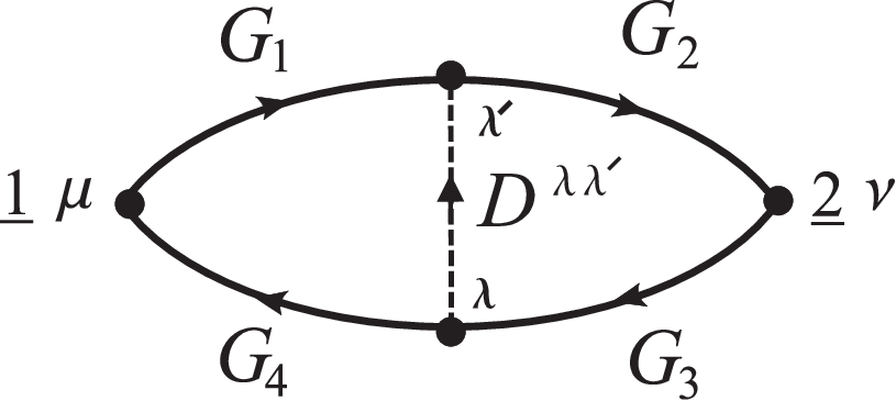
For convenience, we assign indices to the electron Green’s functions as shown in Fig. 7. Then, recalling the expression (2.38) for the bare four-vertex, we have

	$\displaystyle\hskip-20.0pt\left.\Pi_{\mu\nu}(\underline{1}\,\underline{2})\right\|_{\text{2-loop}}=e^{4}D^{\lambda\lambda^{\prime}}(\underline{6}^{\prime}\,\underline{3}^{\prime})$
	$\displaystyle{}\times{\rm tr}_{D}\left\{\delta_{\mu\sigma_{1}}(\underline{1}^{\prime}-\underline{1})\gamma^{\sigma_{1}}\,G_{1}(\underline{1}^{\prime}\,\underline{2}^{\prime})\,\delta_{\lambda^{\prime}\sigma_{2}}(\underline{2}^{\prime}-\underline{3}^{\prime})\gamma^{\sigma_{2}}\,G_{2}(\underline{2}^{\prime}\,\underline{4}^{\prime})\,\right.$
	$\displaystyle\hskip 60.0pt{}\times\left.\delta_{\nu\sigma_{3}}(\underline{4}^{\prime}-\underline{2})\gamma^{\sigma_{3}}\,G_{3}(\underline{4}^{\prime}\,\underline{5}^{\prime})\,\delta_{\lambda\sigma_{4}}(\underline{5}^{\prime}-\underline{6}^{\prime})\gamma^{\sigma_{4}}\,G_{4}(\underline{5}^{\prime}\,\underline{1}^{\prime})\right\}.$		(3.1)

For the polarization functions $\Pi^{<}_{\mu\nu}(12)=\Pi_{\mu\nu}(1_{+}\,2_{-})$ , this formula generates several terms which involve different canonical components of $D^{\lambda\lambda^{\prime}}$ and $G_{i}$ . Let ${\mathcal{P}}^{<}_{\mu\nu}(12)$ be one of these terms with some space-time functions ${\mathcal{D}}^{\lambda\lambda^{\prime}}(12)$ and ${\mathcal{G}}_{i}(12)$ . In the local Wigner form, we obtain (the fixed argument $X$ is omitted for brevity)

	$\displaystyle\hskip-20.0pt{\mathcal{P}}^{<}_{\mu\nu}(k)=\frac{e^{4}}{(2\pi)^{8}}\int d^{4}k^{\prime}\,\prod^{4}_{i=1}d^{4}p_{i}\,\delta^{4}(k-p_{2}+p_{3})\,\delta^{4}(k^{\prime}-p_{3}+p_{4})\,{\mathcal{D}}^{\lambda\lambda^{\prime}}(k^{\prime})$
	$\displaystyle{}\times\delta^{4}(p_{1}+p_{3}-p_{2}-p_{4})\,{\rm tr}_{D}\left\{\hat{\gamma}_{\mu}(k)\,{\mathcal{G}}_{1}(p_{1})\,\hat{\gamma}_{\lambda^{\prime}}(k^{\prime})\,{\mathcal{G}}_{2}(p_{2})\right.$
	$\displaystyle\hskip 170.0pt{}\times\left.\hat{\gamma}_{\nu}(k)\,{\mathcal{G}}_{3}(p_{3})\,\hat{\gamma}_{\lambda}(k^{\prime})\,{\mathcal{G}}_{4}(p_{4})\right\},$		(3.2)

where we have used the notation (4.36). Let us now compare Eq. (3.2) with the one-loop contribution to $\Pi^{<}_{\mu\nu}(X,k)$ that corresponds to the first diagram for $\Pi_{\mu\nu}(\underline{1}\,\underline{2})$ in Fig. 2:

	$\displaystyle\left.\Pi^{<}_{\mu\nu}(k)\right\|_{\text{1-loop}}=-i\,\frac{e^{2}}{(2\pi)^{4}}\int d^{4}p_{1}\,d^{4}p_{2}\,\delta^{4}(k+p_{2}-p_{1})$
	$\displaystyle\hskip 140.0pt{}\times{\rm tr}_{D}\left\{\hat{\gamma}_{\mu}(k)\,G^{<}(p_{1})\,\hat{\gamma}_{\nu}(k)\,G^{>}(p_{2})\right\}.$		(3.3)

A simple analysis based on Eq. (3.1) shows that each term (3.2) involves at least one electron correlation function $G^{<}$ ( ${\mathcal{G}}_{1}(p_{1})$ or ${\mathcal{G}}_{2}(p_{2})$ ), and at least one correlation function $G^{>}$ ( ${\mathcal{G}}_{3}(p_{3})$ or ${\mathcal{G}}_{4}(p_{4})$ ). As discussed in Section 4, the leading approximation for the two-loop contributions to the polarization functions is obtained by replacing $G^{{}^{\gtrless}}(p)$ by their quasiparticle parts $\widetilde{G}^{{}^{\gtrless}}(p)$ which are sharply peaked about the mass-shell. It is clear that, due to the four-dimensional delta functions, the terms (3.2) with products $\widetilde{G}^{<}(p_{1})\,\widetilde{G}^{>}(p_{4})$ and $\widetilde{G}^{<}(p_{2})\,\widetilde{G}^{>}(p_{3})$ correspond to the same scattering process as the one-loop term (3.3) in which $G^{{}^{\gtrless}}$ are replaced by $\widetilde{G}^{{}^{\gtrless}}$ . For weakly coupled plasmas, such two-loop corrections may be neglected¹⁵¹⁵ 15 Examples of the corresponding diagrams for the transverse polarization functions are given in Fig. 4.. On the other hand, the terms (3.2) with $\widetilde{G}^{<}(p_{1})\,\widetilde{G}^{>}(p_{3})$ and $\widetilde{G}^{<}(p_{2})\,\widetilde{G}^{>}(p_{4})$ describe new scattering processes and therefore must be retained. The corresponding diagrams for the transverse polarization functions are shown in Fig. 5.

Appendix D Electromagnetic Energy Production

In the notation of Appendix A, the average electromagnetic energy production in a unit volume due to the interaction with matter can be written as

\frac{\partial{\mathcal{E}}(x)}{\partial t}=-i\big\langle\big[\hat{\mathcal{E}}(x),H_{\rm int}(t)\big]_{-}\big\rangle,

(4.1)

where ${\mathcal{E}}(x)=\langle\hat{\mathcal{E}}(x)\rangle$ and

H_{\rm int}(t)=-\int d^{3}\vec{r}\,\hat{\vec{A}}(x)\cdot\hat{\vec{J}}^{\,T}(x)

is the interaction Hamiltonian. Using the relations (1.2) to calculate the commutator in Eq. (4.1) gives

\frac{\partial{\mathcal{E}}(x)}{\partial t}=\big\langle\hat{\vec{P}}(x)\cdot\hat{\vec{J}}^{\,T}(x)\big\rangle.

(4.2)

We now identify $x$ with the space-time point $X=(T,\vec{R})$ in the kinetic picture and rewrite Eq. (4.2) as

\frac{\partial{\mathcal{E}}(X)}{\partial T}=-\vec{E}(X)\cdot\vec{J}^{\,T}(X)+\left(\frac{\partial{\mathcal{E}}(X)}{\partial T}\right)_{\rm phot},

(4.3)

where $\vec{E}(X)=-\,\partial\vec{A}(X)/\partial T$ is the mean electric field, and $\vec{J}^{\,T}(X)$ is the mean transverse current density. The second term in Eq. (4.3) is associated with photons:

	$\displaystyle\hskip-20.0pt\left(\frac{\partial{\mathcal{E}}(X)}{\partial T}\right)_{\rm phot}=\frac{1}{2}\int d^{4}x_{1}\,d^{4}x_{2}\,\delta^{4}(x_{1}-X)\,\delta^{4}(x_{2}-X)$
	$\displaystyle\hskip 85.0pt{}\times\frac{\partial}{\partial t_{2}}\left[\big\langle\Delta\hat{J}^{\,T}_{i}(1)\,\Delta\hat{A}_{i}(2)\big\rangle+\big\langle\Delta\hat{A}_{i}(2)\,\Delta\hat{J}^{\,T}_{i}(1)\big\rangle\right],$		(4.4)

where $\Delta\hat{J}^{\,T}_{i}(1)=\hat{J}^{\,T}_{i}(x_{1})-{J}^{\,T}_{i}(x_{1})$ and $\Delta\hat{A}_{i}(2)=\hat{A}_{i}(x_{2})-{A}_{i}(x_{2})$ . The correlation functions in the above formula can be written in terms of the field Green’s functions and the polarization functions by noting that

\frac{1}{\langle S\rangle}\,\big\langle T_{C}\big\{S\,\Delta\hat{J}^{\,T}_{Ii}(\underline{1})\,\Delta\hat{A}_{Ij}(\underline{2})\big\}\big\rangle=i\,\frac{\delta J^{T}_{i}(\underline{1})}{\delta J^{\,(\text{ext})j}(\underline{2})}=-i\,\Pi_{ij^{\prime}}(\underline{1}\,\underline{1}^{\prime})\,D_{j^{\prime}j}(\underline{1}^{\prime}\,\underline{2})

as follows directly from Eqs. (2.5) and (2.6). In the physical limit one obtains

	$\displaystyle\big\langle\Delta\hat{J}^{\,T}_{i}(1)\,\Delta\hat{A}_{i}(2)\big\rangle=-i\left[\pi^{>}_{ij}(11^{\prime})\,d^{-}_{ji}(1^{\prime}2)+\pi^{+}_{ij}(11^{\prime})\,d^{>}_{ji}(1^{\prime}2)\right],$
	$\displaystyle\big\langle\Delta\hat{A}_{i}(2)\,\Delta\hat{J}^{\,T}_{i}(1)\big\rangle=-i\left[\pi^{+}_{ij}(11^{\prime})\,d^{<}_{ji}(1^{\prime}2)+\pi^{<}_{ij}(11^{\prime})\,d^{-}_{ji}(1^{\prime}2)\right].$

After inserting these expressions into Eq. (4.4) we use the rule (3.7) to express all functions in terms of their Wigner transforms, and then go over to the principal-axis representation (3.27). These manipulations give (on the right-hand side the $X$ -dependence is not shown explicitly)

	$\displaystyle\hskip-20.0pt\left(\frac{\partial{\mathcal{E}}(X)}{\partial T}\right)_{\rm phot}=-\,\frac{i}{2}\sum_{s}\int\frac{d^{4}k}{(2\pi)^{4}}\left(\frac{1}{2}\,\frac{\partial}{\partial T}+ik_{0}\right)$
	$\displaystyle\hskip 50.0pt{}\times\left[\pi^{+}_{s}(k)\big(d^{>}_{s}(k)+d^{<}_{s}(k)\big)+\big(\pi^{>}_{s}(k)+\pi^{<}_{s}(k)\big)d^{-}_{s}(k)\right].$		(4.5)

Here the contributions from the Poisson brackets have been omitted since they are small in the kinetic regime. For the same reason, the term with the derivative $\partial/\partial T$ can be neglected since it gives a relatively small correction to the energy density ${\mathcal{E}}(X)$ , which is unimportant for our present purposes. The remaining integral in Eq. (4.5) represents the photon contribution to the local electromagnetic energy balance. With the symmetry relations for the transverse functions

	$\displaystyle d^{{}^{\gtrless}}_{s}(X,-k)=d^{{}^{\lessgtr}}_{s}(X,k),\qquad\pi^{{}^{\gtrless}}_{s}(X,-k)=\pi^{{}^{\lessgtr}}_{s}(X,k),$
	$\displaystyle d^{\pm}_{s}(X,-k)=d^{\mp}_{s}(X,k),\qquad\pi^{\pm}_{s}(X,-k)=\pi^{\mp}_{s}(X,k),$

we get the expression in which the integration is over $k_{0}>0$ :

\left(\frac{\partial{\mathcal{E}}(X)}{\partial T}\right)_{\rm phot}=\sum_{s}\int\frac{d^{4}k}{(2\pi)^{4}}\,\theta(k_{0})k_{0}\left[\pi^{>}_{s}(X,k)d^{<}_{s}(X,k)-\pi^{<}_{s}(X,k)d^{>}_{s}(X,k)\right].

Recalling the decomposition (3.33), we see that here the field correlation functions ${d}^{{}^{\gtrless}}_{s}(X,k)$ can be replaced by their resonant parts $\widetilde{d}^{\,{}^{\gtrless}}_{s}(X,k)$ . Then, using the relations (3.41) and (3.43) leads to Eq. (6.1).

Appendix E Photon Dispersion

The dispersion relation for photons follows from Eq. (3.48). To solve this equation, one needs an explicit expression for ${\rm Re}\,\pi^{+}_{s}(X,k)$ . We start with the space-time functions $\pi^{\pm}_{ij}(12)$ which can be written in terms of the transverse polarization matrix $\Pi_{ij}(\underline{1}\,\underline{2})$ . Recalling the canonical notation (2.2) for functions on the contour $C$ , we have

\pi^{\pm}_{ij}(12)=\pm\,\Pi_{ij}(1_{\pm}\,2_{\pm})\mp\,\Pi_{ij}(1_{+}\,2_{-}).

(5.1)

Here it is sufficient to retain only the contribution of the one-loop diagram (see Fig. 2) that dominates in the case of a weakly coupled plasma. Then the functions (5.1) are given by the space-time diagrams

\pi^{\pm}_{ij}(12)=\,\raisebox{-26.0pt}{\includegraphics[scale={0.4}]{NewLoops12.eps}}

(5.2)

Going over to the local Wigner representation and using the first of Eqs. (3.24), we obtain

	$\displaystyle\hskip-15.0pt{\rm Re}\,\pi^{+}_{ij}(X,k)=-ie^{2}\Delta^{\perp}_{ii^{\prime}}(\vec{k})\,\Delta^{\perp}_{jj^{\prime}}(\vec{k})$
	$\displaystyle\hskip 20.0pt{}\times\int\frac{d^{4}p}{(2\pi)^{4}}\,{\rm tr}_{D}\left\{\gamma^{i^{\prime}}\left[g(X,p+k)+g(X,p-k)\right]\gamma^{j^{\prime}}\,G^{<}(X,p)\right\},$		(5.3)

where $\Delta^{\perp}_{ii^{\prime}}(\vec{k})$ is the transverse projector (3.16), and

g(X,p)=\frac{1}{2}\left[g^{+}(X,p)+g^{-}(X,p)\right].

Note that in Eq. (5.3) the off-shell part of $G^{<}(X,p)$ must be dropped since it gives the contribution of the same order as the two-loop diagram in Fig. 2, which has been neglected. In other words, the full function $G^{<}(X,p)$ is to be replaced by its quasiparticle part $\widetilde{G}^{<}(X,p)$ . To the leading approximation for a weakly coupled plasma, the local propagators $g^{\pm}(X,p)$ and the correlation functions $\widetilde{G}^{<}(X,p)$ may be taken in the collisionless form, Eqs. (4.16) and (4.27). Then, by changing the integration variable $p$ into $p+eA(X)$ , the polarization tensor (5.3) is expressed in terms of the gauge-invariant distribution functions (4.31). After some algebra, we have

	$\displaystyle{\rm Re}\,\pi^{+}_{ij}(X,k)=8\pi e^{2}\Delta^{\perp}_{ij}(\vec{k})$
	$\displaystyle{}\times\int\frac{d^{4}p}{(2\pi)^{4}}\left[1+\frac{k^{4}}{4}\cdot\frac{\wp}{(p\cdot k)^{2}-k^{4}/4}\right]\eta(p^{0})\,\delta\big(p^{2}-m^{2}\big)f^{<}(X,p)$
	$\displaystyle-8\pi e^{2}k^{2}\,\Delta^{\perp}_{ii^{\prime}}(\vec{k})\Delta^{\perp}_{jj^{\prime}}(\vec{k})$
	$\displaystyle{}\times\int\frac{d^{4}p}{(2\pi)^{4}}\,\frac{\wp}{(p\cdot k)^{2}-k^{4}/4}\,p_{i^{\prime}}p_{j^{\prime}}\,\eta(p^{0})\,\delta\big(p^{2}-m^{2}\big)f^{<}(X,p),$		(5.4)

where $\wp$ denotes the principal values of integrals. Two comments are relevant concerning the above expression. First, it should be noted that ${\rm Re}\,\pi^{+}_{ij}(X,k)$ contains a divergent vacuum term which is to be eliminated by applying the procedure of vacuum QED (for a discussion of this point see Bezzerides and DuBois [24]). In what follows we ignore this vacuum term, assuming the physical mass and charge throughout. Second, for experimental conditions available at present, the positron contribution to $f^{<}(X,p)$ may be neglected in calculating ${\rm Re}\,\pi^{+}_{ij}(X,k)$ . Therefore, in Eq. (5.4) we shall make the replacement

\eta(p^{0})\,\delta\big(p^{2}-m^{2}\big)f^{<}(X,p)=\frac{\delta\big(p^{0}-E_{p}\big)}{2E_{p}}\,f(X,\vec{p}),

(5.5)

where $E_{p}=\sqrt{\displaystyle|\vec{p}\,|^{\,2}+m^{2}}$ , and $f(X,\vec{p})\equiv f_{e^{-}}(X,\vec{p})$ is the electron distribution function.

The next step is to find eigenvectors and eigenvalues of the polarization tensor (5.4). In general this is a rather complicated problem which requires a knowledge of the nonequilibrium particle distribution functions. Note, however, that our main interest is in the region of sufficiently high frequencies $\omega=|k^{0}|$ where the dispersion curve for transverse photons is close to the vacuum limit $\omega=|\vec{k}|$ . Since in this region the quantity $k^{2}=\omega^{2}-\vec{k}^{\,2}$ is small compared to $\omega^{2}$ , a simple and reasonable approximation for the polarization tensor can be obtained from Eq. (5.4) by setting $k^{2}=0$ . Taking also Eq. (5.5) into account, we obtain a locally isotropic tensor

{\rm Re}\,\pi^{+}_{ij}(X,k)=\omega^{2}_{e}(X)\left(\delta_{ij}-\frac{k_{i}k_{j}}{|\vec{k}|^{2}}\right)

(5.6)

with $\omega_{e}(X)$ defined in Eq. (6.4). In this case ${\rm Re}\,\pi^{+}_{s}(X,k)=\omega^{2}_{e}(X)$ , so that the dispersion equation (3.48) reduces to $k^{2}-\omega^{2}_{e}(X)=0$ , whence follows the expression (6.5) for the effective photon frequencies. If $\omega^{2}\gg\omega^{2}_{e}$ , the anisotropic corrections to the polarization tensor (5.4) are relatively small. The leading anisotropic contribution comes from the last term and is given by

	$\displaystyle\hskip-15.0pt\left.{\rm Re}\,\pi^{+}_{ij}(X,k)\right\|_{\rm anisotr}=-4\pi e^{2}k^{2}\,\Delta^{\perp}_{ii^{\prime}}(\vec{k})\Delta^{\perp}_{jj^{\prime}}(\vec{k})$
	$\displaystyle\hskip 80.0pt{}\times\int\frac{d^{4}p}{(2\pi)^{4}}\,\frac{\wp}{(p\cdot k)^{2}}\,p_{i^{\prime}}p_{j^{\prime}}\,\frac{\delta\big(p^{0}-E_{p}\big)}{E_{p}}\,f(X,\vec{p}),$		(5.7)

where we have used Eq. (5.5).

Appendix F Longitudinal Field Correlation Functions

We start with the equation of motion for the longitudinal field Green’s function $D(\underline{1}\,\underline{2})\equiv D^{00}(\underline{1}\,\underline{2})$ on the time-loop contour $C$ . Recalling Eqs. (2.24) and (2.49), we have

-\nabla^{2}_{1}D(\underline{1}\,\underline{2})=\delta(\underline{1}-\underline{2})+\Pi(\underline{1}\,\underline{1}^{\prime})D(\underline{1}^{\prime}\,\underline{2}).

(6.1)

The adjoint of this equation reads

-\nabla^{2}_{2}D(\underline{1}\,\underline{2})=\delta(\underline{1}-\underline{2})+D(\underline{1}\,\underline{1}^{\prime})\Pi(\underline{1}^{\prime}\,\underline{2}).

(6.2)

Then, using the canonical form (2.2) of $D(\underline{1}\,\underline{2})$ and $\Pi(\underline{1}\,\underline{2})$ , it is an easy matter to derive the equations for the retarded and advanced longitudinal “propagators”


	$\displaystyle-\nabla^{2}_{1}D^{\pm}(12)=\delta(1-2)+\Pi^{\pm}(11^{\prime})D^{\pm}(1^{\prime}2),$		(6.3a)
	$\displaystyle-\nabla^{2}_{2}D^{\pm}(12)=\delta(1-2)+D^{\pm}(11^{\prime})\Pi^{\pm}(1^{\prime}2),$		(6.3b)

and the KB equations for the space-time correlation functions


	$\displaystyle-\nabla^{2}_{1}D^{{}^{\gtrless}}(12)=\Pi^{+}(11^{\prime})D^{{}^{\gtrless}}(1^{\prime}2)+\Pi^{{}^{\gtrless}}(11^{\prime})D^{-}(1^{\prime}2),$		(6.4a)
	$\displaystyle-\nabla^{2}_{2}D^{{}^{\gtrless}}(12)=D^{{}^{\gtrless}}(11^{\prime})\Pi^{-}(1^{\prime}2)+D^{+}(11^{\prime})\Pi^{{}^{\gtrless}}(1^{\prime}2).$		(6.4b)

The analysis of the above equations proceeds exactly in parallel with that for the transverse field fluctuations. By going over to the Wigner representation (3.6) and keeping only first order terms in the $X$ -gradients, the sum and difference of Eqs. (6.3) become

\left({\vec{k}}^{\,2}-\Pi^{\pm}(X,k)\right)D^{\pm}(X,k)=1,\qquad\left\{\vec{k}^{\,2}-\Pi^{\pm}(X,k),D^{\pm}(X,k)\right\}=0,

(6.5)

whence

D^{\pm}(X,k)=\frac{1}{{\vec{k}}^{\,2}-\Pi^{\pm}(X,k)}.

(6.6)

In the Wigner representation, the KB equations (6.4) are manipulated to

	$\displaystyle\hskip-15.0pt\left\{{\vec{k}}^{\,2}-{\rm Re}\,\Pi^{+},D^{{}^{\gtrless}}\right\}+\left\{{\rm Re}\,D^{+},\Pi^{{}^{\gtrless}}\right\}=i\left(\Pi^{>}D^{<}-\Pi^{<}D^{>}\right),$		(6.7)
	$\displaystyle\hskip-15.0pt\left\{{\rm Im}\,\Pi^{+},D^{{}^{\gtrless}}\right\}+\left\{{\rm Im}\,D^{+},\Pi^{{}^{\gtrless}}\right\}=2\left({\vec{k}}^{\,2}-{\rm Re}\,\Pi^{+}\right)\left(D^{{}^{\gtrless}}-\|D^{+}\|^{2}\,\Pi^{{}^{\gtrless}}\right),$		(6.8)

where the arguments $X$ and $k$ are omitted for brevity. Equation (6.7) is derived by taking the difference of Eqs. (6.4) and may be regarded as the transport equation for longitudinal field fluctuations. It is quite similar in structure to the plasmon transport equation in nonrelativistic plasmas [25]. Equation (6.8) is analogous to the mass-shell equation (3.28b) for transverse field fluctuations.

References

[1] D. Gordon et al., Phys. Rev. Lett. 80, 2133 (1998).
[2] C.E. Clayton et al., Phys. Rev. Lett. 81, 100 (1998).
[3] M.I.K. Santala et al., Phys. Rev. Lett. 86, 1227 (2001).
[4] S.P.D. Mangles et al., Phys. Rev. Lett. 94, 245001 (2005).
[5] E.L. Clark et al., Phys. Rev. Lett. 84, 670 (2000).
[6] E.L. Clark et al., Phys. Rev. Lett. 85, 1654 (2000).
[7] R.A. Snavely et al., Phys. Rev. Lett. 85, 2945 (2000).
[8] J.B. Rosenzweig et al., Phys. Rev. A 44, R6189 (2004).
[9] A. Pukhov, Z-M. Sheng, and J. Meyer-ter-Vehn, Phys. Plasmas 6, 2847 (1999).
[10] F.S. Tsung et al., Phys. Rev. Lett. 93, 185002 (2004).
[11] M. Honda, J. Meyer-ter-Vehn, and A. Pukhov, Phys. Rev. Lett. 85, 2128 (2000).
[12] A. Bret, M-C. Firpo, and C. Deutsch, Phys, Rev. E 70, 04641 (2004).
[13] J.T. Mendonça et al., Phys. Rev. Lett. 94, 245002 (2005).
[14] R.C. Tautz, R. Schlickeiser, and I. Lerche, J. Math. Phys. 48, 013302 (2007).
[15] S. Klein, Rev. Mod. Phys. 71, 1501 (1999).
[16] M.I.K. Santala et al., Phys. Rev. Lett. 84, 1459 (2000).
[17] S.R. de Groot, W.A. van Leeuwen, Ch.G. van Weert, Relativistic Kinetic Theory. Principles and Applications (North-Holland Publishing Company, Amsterdam-New York-Oxford, 1980).
[18] D.N. Zubarev, V.G. Morozov, and G. Röpke, Statistical Mechanics of Nonequilibrium Processes, Vol. 1 (Akademie Verlag, Berlin, 1996).
[19] D.N. Zubarev, V.G. Morozov, and G. Röpke, Statistical Mechanics of Nonequilibrium Processes, Vol. 2 (Akademie Verlag, Berlin, 1997).
[20] M. Bonitz, Quantum Kinetic Theory (Teubner, Stuttgart-Leipzig, 1998).
[21] L.P. Kadanoff and G. Baym, Quantum Statistical Mechanics (Benjamin, New York, 1962).
[22] P. Danielewicz, Ann. Phys. (N.Y.) 152, 239 (1984).
[23] W. Botermans and R. Malfliet, Phys. Rep. 198, 115 (1990).
[24] B. Bezzerides and D.F. DuBois, Ann. Phys. (N.Y.), 70, 10 (1972).
[25] D.F. DuBois, in Lectures in Theoretical Physics, edited by W.E. Brittin, (Gordon and Breach, New York, 1967) pp. 469-619.
[26] H.S. Köhler and R. Malfliet, Phys. Rev. C 48, 1034 (1993).
[27] V. Špička and P. Lipavský, Phys. Rev. Lett. 73, 3439 (1994).
[28] V. Špička and P. Lipavský, Phys, Rev. B 52 (20), 14615 (1995).
[29] Th. Bornath, D. Kremp, W.D. Kraeft, and M. Schlanges, Phys, Rev. E 54, 3274 (1996).
[30] D. Kremp, M. Schlanges, and Th. Bornath, J. Stat. Phys. 41, 661 (1985).
[31] V.G. Morozov and G. Röpke, Ann. Phys. (N.Y.) 278, 127 (1999).
[32] B. Vanderheyden and G. Baym, J. Stat. Phys. 93, 843 (1998).
[33] C. Itzykson and J.-B. Zuber, Quantum Field Theory (McGraw-Hill, New York, 1980).
[34] St. Mrówczyński and U. Heinz, Ann. Phys. (N.Y.), 229, 1 (1994).
[35] E. Quack and P.A. Henning, Phys. Rev. D 54, 3125 (1996).
[36] P. Aurenche, F. Gelis, R. Kobes, and E. Petitgirard, Z. Phys. C 75, 315 (1997).
[37] P. Aurenche, F. Gelis, and H. Zaraket, Phys. Rev. D 62, 096012 (2000).
[38] V.G. Morozov and G. Röpke, Cond. Matt. Phys. 9, No 3(47), 473 (2006).
[39] M. Tatarakis et al., Phys. Rev. Lett. 90, 175001 (2003).
[40] F.C. Jones, Phys. Rev. 167, 1159 (1968).
[41] G.R. Blumenthal and R.J. Gould, Rev. Mod. Phys. 42, 237 (1970).
[42] A.G. Pacholczyk, Radio Astrophysics (Freeman, San Francisco, 1970).
[43] P.S. Yeung and R.L. Brown, Phys. Rev. D 8, 4286 (1973).
[44] B. Altschul, Phys. Rev. D 75, 041301 (2007).
[45] S. Profumo, Phys. Rev. D 77, 103510 (2008).
[46] J. Braun and H.-J. Pirner, Phys. Rev. D 75, 054031 (2007).
[47] V.N. Tsytovich, Theory of Turbulent Plasma (Plenum, Oxford, 1977).
[48] B.B. Kadomtsev, Plasma Turbulence (Academic, N.Y., 1965).
[49] A. Gailitis and V.N. Tsytovich, Sov. Phys.-JETP 19, 1165 (1964).
[50] V.N. Tsytovich, Phys. Rep. 178, 261 (1989).
[51] K.G. Kato, G. Benford, and D. Tzach, Phys. Fluids 26, 3636 (1983).
[52] D.L. Newman, Phys. Fluids 28 1482 (1985).
[53] Yu.B. Ivanov, J. Knoll, and D.N. Voskresensky, Yad. Fiz. 66, 1950 (2003) [Phys. At. Nucl. 66, 1902 (2003)].
[54] A. Pukhov, Rep. Prog. Phys. 66, 47 (2003).
[55] C. Ren et al., Phys. Rev. Lett. 93, 185004 (2004).
[56] P. Antici et al., Phys. Rev. Lett. 101, 105004 (2008).
[57] S. Weinberg, The Quantum Theory of Fields, Vol. 1 (Cambridge University Press, Cambridge UK, 1995).