Anomaly-Mediated Supersymmetry Breaking Demystified
Abstract:
We reinterpret anomaly-mediated supersymmetry breaking from a field-theoretic perspective in which superconformal anomalies couple to either the chiral compensator or the vector superfield. As supersymmetry in the hidden sector is spontaneously broken by non-vanishing vacuum expectation values of the chiral compensator F-term and/or the vector superfield D-term, the soft breakdown of supersymmetry emerges in the visible sector. This approach is physically more understandable compared with the conventional approach where the chiral compensator is treated on the same footing as a spurion in gauge-mediated supersymmetry breaking scenario.
Keywords:
superconformal anomaly, supersymmetry breaking1 Introduction
The intensive study for the TeV scale physics is just around the corner thanks to the LHC. Many candidates of new physics beyond the Standard Model are about to be put to test as the LHC spawns a bonanza of new experimental data in the coming years. Soon after the first analysis arrives, many candidates will be immediately ruled out but some will survive the test. This procedure goes on as the opreation of the LHC continues. Supersymmetry is the most promising candidate to survive the LHC test. There are more reasons to support supersymmetry as the LHC’s choice. Supersymmetry provides a promising solution to the hierarchy problem, explains unification of gauge coupling constant, and encompasses a candidate for furtive dark matter of the Universe. All the three issues are the most urgent problems in particle physics.
Without question, supersymmetry is not found at least up to weak energy scale. It is believed tht supersymmetry is spontaneously broken in the hidden sector at some high energy scale and then its breaking is mediated to the visible sector, leading to the soft terms of the MSSM. Three prominent mechanisms for the mediation of supersymmetry breaking are Planck-scale-mediated 11 1 It is also referred to as gravity-mediated, which is an improper use of terminology., gauge-mediated and anomaly-mediated supersymmetry breaking (PMSB, GMSB, and AMSB). In this article we concentrate on AMSB scenario. Here the anomaly refers to superconformal anomaly and the history of its study goes back to mid 1970’s along with developments in rigid supersymmetry theories [1].
Though superconformal symmetry is classically preserved in theories without dimensionful parameters it is in general broken by the quantum effects. Interestingly, the resultant superconformal anomalies constitute distinct types of supermultiplet by themselves. There are at least two kinds of superconformal anomaly supermultiplets - the chiral anomaly and linear anomaly. The former contains three anomalies - trace anomaly, anomaly and local conformal supersymmetry anomaly while the latter encompasses only two anomalies (along with a conserved current) - trace anomaly and local conformal supersymmetry anomaly. Each anomaly supermultiplet couples to a distinctive superfield in Einstein supergravity. Though the superconformal anomalies do not break supersymmetry by themselves, the coupling of the superconformal anomalies to the superfields in supergravity play as a mediator of supersymmetry breaking from the hidden sector to the visible sector.
In the conventional AMSB scenario [2, 3] based on the lagrangian of the coupled matter-supergravity system in ref. [4, 5], the chiral compensator22 2 It is also referred to as the Weyl compensator or the conformal compensator. plays a central role not only as the mediator of supersymmetry breaking but also as the superfield spurion whose auxiliary component sets the supersymmetry-breaking mass scale. It is distinguishable from the GMSB scenario where the two roles are played separately by the two different superfields - the goldstino spurion and gauge messenger(s). On the other hand, in PMSB scenario the superfield spurion is played by a SM-singlet superfield of the hidden sector.
In this article we interpret the chiral compensator as a supersymmetric extension of the Nambu-Goldstone boson (NGB) associated with broken superconformal symmetry. With this interpretation we understand that the compensator not only plays the two distinctive roles simultaneously but also is regarded as the invariant measure of chiral superspace in supergravity. This leads to the coupling of the chiral compensator to the chiral anomaly supermultiplet [1] through the quantum effects. When the F-term vacuum expectation value (VEV) of the chiral compensator is turned on by the supersymmetry breaking in the hidden sector [6], the soft breaking of supersymmetry in the visible sector emerges through the chiral anomaly supermultiplet. Therefore the soft parameters of the visible sector are characterized both by the F-term VEV and by the beta function associated with superconformal anomalies.
As the chiral anomaly supermultiplet couples to the chiral compensator the linear anomaly supermultiplet [7, 8, 9] also couples to a superfield which is referred to as the vector superfield. This concurs with a supersymmetrization of the coupling of -current to the gauge field. In a similar manner to the chiral compensator, the vector superfield forms a genuine vector superfield. When the D-term of the vector superfield gets a non-vanishing VEV due to the hidden sector [6], the soft terms in the visible sector take place as well.
The article is organized as follows. In Section 2, we briefly review key ideas on the connection between conformal symmetry and gravity. In Section 3, we set up the chiral anomaly supermultiplet and chiral compensator, and then find the coupling between them. In Section 4, we establish the linear anomaly supermultiplet and vector superfield, and then acquire the coupling between them. In Section 5, the connection between the anomaly supermultiplet and supercurrent is demonstrated with the massless interacting Wess-Zumino model. In Section 6, we explain how to spawn the soft terms of the visible sector through the AMSB mechanism. In Section 7, we summarize the article with the outlook for the future works. Finally, there are four Appendices which elucidate how to evaluate the (super)conformal anomalies using (superspace) perturbation theory and (super)graphs.
2 Conformal symmetry and gravity
Let us consider the conformal symmetry in massless QCD. If all the quarks in QCD were massless then the theory would contain no dimensional parameters in the lagrangian,
| (1) |
and it would exhibit a classical scale invariance. For conformal (or scale) transformations where is arbitrary but real, the associated quark and gluon scale transformations would be
| (2) | |||||
| (3) |
These lead to a traceless energy-momentum tensor, with conserved dilatation current ,
| (4) |
where is the energy-momentum tensor.
But conformal symmetry is broken by the quantum effects. For instance, dimensional regularization imperatively brings about a renormalization mass scale which naturally introduces a dimensionful parameter to the theory, and therefore breaks conformal symmetry. Whenever a global symmetry is spontaneously broken the associated NGB takes place. The NGB for the broken conformal symmetry is referred to as the dilaton, denoted by from now. The dilaton couples to the trace of energy-momentum tensor , leading to an effecive action (see Appedix A for how to evaluate it):
| (5) | |||||
| (6) |
where is the beta function for QCD. is referred to as the conformal (or trace) anomaly. The effective action is regarded as the coupling of a source (conformal anomaly) to an external field (dilaton) from a field-theoretic viewpoint.
The effective action (5) can be viewed in a different perspective. If the gluon field is rescaled to , then the effective action is written as
| (7) |
That is, renormalization of the gluon field turns the effective action into the coupling of the dilaton to the lagrangian for the YM theory. As flat space is extended to curved space, the global parameter in flat space transmutes into the dynamical field in curved space. Indeed in (5) is an integral measure in Einstein gravity where gravity couples to energy-momentum tensor. It is the crossing point where Einstein gravity and quantum field theory without gravity confront in order to deal with conformal symmetry.
When gravity embraces supersymmetric matter, Einstein gravity is extended to Einstein supergravity. Likewise, conformal symmetry is extended to superconformal symmetry. Nonetheless conformal symmetry is broken at the quantum level and so is superconformal symmetry. As broken conformal symmetry generates a dilaton, broken superconformal symmetry brings about not only a dilaton but also its superpartner, dilatino. Moreover, both the dilaton and dilatino constitute a supermultiplet. We have already shown that a dilaton couples to quantum conformal anomaly. In the following two sections, we will extend the coupling of a dilaton to conformal anomaly to superspace - quantum superconformal anomalies form a supermultiplet and couples to the dilaton superfield. We will analyze two kinds of superconformal anomaly supermultiplets and then identify the corresponding dilaton superfields.
3 Chiral anomaly supermultiplet and chiral compensator
In conformal supergravity [10] all the relevant dynamical contents are encoded in a single gravitational superfield (i.e. in the Wess-Zumino gauge) as
| (8) |
Here and are a gauge transformations, vierbein and gravitino, respectively, and their degrees of freedom are three, five and eight, respectively. As for we remove one degree of freedom for the local -symmetry out of four so the three degrees of freedom turn out to form the gauge field. As for we subtract six degrees of freedom corresponding to local Lorentz invariance, and four degrees of freedom corresponding to general coordinate invariance, and one degree of freedom corresponding to dilatations. Similarly, as for we take off four degrees of freedom for local supersymmetry generators by and , and four degrees of freedom for local conformal supersymmetry generators and .
The conformal supergravity multiplet [10] couples to the supercurrent multiplet [1] - energy momentum tensor , supersymmetry current (along with its conjugate, )33 3 It is also referred to as spin- supercurrent in ref. [11]. and -current . When the supercurrent satisfies the conservation equations
| (9) |
its components form a (real scalar) supermultiplet. It can be easily read off from the fact that the degrees of freedom for and are three, five and eight, respectively. Recall that the supercurrent is not local but global current. Thus in rigid supersymmetry theories the superconformal gravity multiplets are treated as external fields for the supercurrent (we will exhibit it in Section 5). We apply the current-external-field relation to superconformal anomalies and superfield in Einstein supergravity as well.
We suppose that all the three symmetries are anomalous. That is, none of the three conservation equations is satisfied:
| (10) |
The degrees of freedom for the anomalies and turn out to be four, one and one, respectively. To become a supermultiplet we need two new bosonic degrees of freedom, denoted by and . They are auxiliary components. What’s more, the four bosonic degrees of freedom are divided into two distinct groups which contain two degrees of freedom each. It implies that the supermultiplet is chiral. The anomaly is referred to as the chiral anomaly supermultiplet (CASM) [12]:
| (11) |
where and . In contrast to a genuine chiral superfield which has auxiliary fields as the -component, the CASM places them at the zero-component, a fact which will have an immediate consequence for supersymmetry breaking. Since we know the mass dimension of conformal anomaly and/or supersymmetry anomaly, (, ), we find . Moreover the trace and anomalies go in pairs [13] so as to become complex. For instance, in SYM theory the trace anomaly is given as while the anomaly as . We will comment on it at the end of this section.
Let us figure out the superfield which couples to the CASM. As shown in Section 2, the trace anomaly should couple to the dilaton, . Similarly, the anomaly should couple to the degree of freedom for the local -symmetry. From a field-theoretic point of view, it is the NGB arising from the broken symmetry. We denote it as from now. The supersymmetry anomaly should couple to dilatino which couples to the degrees of freedom for the local conformal supersymmetry generators (approximately ). These all simply reinforce the fact that the Nambu-Goldstone bosons or fermions arising from broken global symmetries in rigid supersymmetric theories agree with the degrees of freedoms for broken local symmetries in supergravity. Nonetheless we need two more bosonic degrees of freedom to balance the bosonic and fermionic degrees of freedom. They are not associated with any symmetries so that they are auxiliary fields that couple to in (11) [14, 15]. Thus these four bosonic and four fermionic degrees of freedom are accommodated in a chiral superfield of the form [16]
| (12) |
where is complex. It is interesting to note that the role of the Bose components in the chiral compensator is reveresed by that of the CASM. This superfield is referred to as the chiral compensator. The mass dimension of the chiral compensator and its components are and .
In addition to constituting a chiral superfield, the chiral compensator plays a role in supergravity. As previously mentioned, it is eaten by the gravitational superfield , whose degrees of freedom are thereby increased by four, one, one, respectively. Moreover, to be a complete multiplet, the gravitational superfield also contains .
In Einstein supergravity, the chiral compensator is defined as an invariant measure in chiral superspace
| (13) |
We can comprehend this property by decomposing the chiral compensator as
| (14) |
Note that the term in the first curly bracket is the invariant measure in general relativity without supersymmetry while the first term in the second curly bracket is the integral measure in -space. is the phase associated with the local rotations. By rotating the phase can disappear in -space. But the rotation transforms and , respectively, as
| (15) | |||||
| (16) |
so the chiral compensator is not uniquely defined. This illustrates that the chiral compensator is covariant under a gauge group - the local rotations. This is a supergravity aspect. Therefore the local rotations in supergravity are anything but the global rotations in rigid supersymmetry theories so that the CASM components transform under the rotations as
| (17) | |||||
| (18) | |||||
| (19) |
We are ready to build up the coupling of the chiral compensator to the CASM. We utilize the properties of CASM and chiral compensator that we have found so far. The mass dimension of the CASM and the chiral compensator are three and zero, respectively, and the chiral compensator plays a role as an integral measure in chiral superspace. Moreover, we have already described how the components of the CASM couple to the components of the chiral compensator in advance. Thus it is not difficult to figure out an action of the form
| (20) |
For instance, we can come up with the same action by extending the effective action in (7) to superspace.
Let us view the action from the aspect of effective field theory. A genuine chiral superfield in rigid supersymmetry theories is achieved by multiplying the chiral compensator by a mass parameter which is assumed be the Planck mass. Then the chiral superfield is explicitly written as
| (21) | |||||
At much low energy scale (i.e. weak scale), the dilaton has no VEV () while is unknown. Therefore the component is given by at low energy scale. In this regard we fathom why is a complex auxiliary field. The action is rewritten as
| (22) |
It is a nonrenormalizable interaction suppressed by the Planck mass due to and . If has a non-vanishing VEV, (with ), then the action leads to soft terms in the visible sector. In this regard, we would say that anomaly mediation is regarded as Planck-scale-mediation.
Before ending up this section we would like to make a few comments on the action with regard to the rotations. Expanding the action (20) in components, we have
| (23) |
Let us consider the action in the limit . The first term leads to soft supersymmetry breaking terms in the visible sector if acquires a non-vanishing VEV. The second term represents the coupling of the dilatino (gravitino) to the supersymmetry anomaly. The third term is associated with both conformal and anomalies - the conformal anomaly survives while the anomaly fade away. The more interesting setup is that has a non-vanishing VEV, , regardless of . It triggers anomalies which are proportional to . For instance, in YM theory it brings in the term. The most interesting situation is that is a dynamical field like . It is anything but an axion arising from anomaly mediation. We will not discuss it in this article. Studies on phenomenologies of the axion arising from anomaly mediation under current investigation [17].
4 Linear anomaly supermultiplet and vector superfield
In this section we will address a new superconformal anomaly (superfield). To begin with, let us return to the three conservation equations (9). We now assume that only -current is still conserved but the other two currents become anomalous,
| (24) | |||
| (25) |
and then the degrees of freedom for and are one and four, respectively. To constitute a superfield, three new bosonic degrees of freedom are needed. is the conserved current for the global transformations in rigid supersymmetric theories (or for the local gauge transfortions in supergravity). Moreover, the degrees of freedom for are three, as shown in Section 3. Taking the two hints, we can figure out that the new three bosonic degrees of freedom are indeed . This in turn verifies that the anomaly supermultiplet is linear. It is referred to as the linear anomaly supermultiplet (LASM)44 4 It contains the same degrees of freedom with the tensor multiplet [19] where an antisymmetric-tensor gauge field takes the place of the gauge field in the linear superfield. in ref. [7, 8].
Let us identify the LASM components with its corresponding degrees of freedom. Using the most general expression for a real linear superfield, we can write down the LASM in terms of its power series expansion in and [16]:
| (26) | |||||
All the components are expressed by , and . Moreover, the -current is assigned to the -component, as expected. It is interesting to note that LASM has the field content of a vector superfield. However the roles of the Bose components of the LASM, compared with a vector field, are reversed: the scalar is now physical (instead of auxiliary), and the transverse vector now has one physical component and two auxiliary components (instead of two physical and one auxiliary). With a knowledge of we read off the mass dimension of its components - , and . Therefore we can identify the degrees of freedoms for (conformal anomaly) and (supersymmetry anomaly) with and , respectively.
Let us look for the superfield corresponding to the LASM. From a field-theoretic perspective, there must be an external vector field which couples to the -current. On the other hand, gravitational superfield encompasses the vector field as components, which is explained in Section 3 (when we count the degrees of freedom for the gravitational superfield (8)). Thus the vector field, , is transmuted into the vector superfield, . Using the following supersymmetric generalization of gauge transformations:
| (27) |
with being a chiral field , we construct the most general expression for written in terms of its power series expansion in and :
| (28) | |||||
Checking out mass dimension of its components, we come up with , , and . In the Wess-Zumino gauge where , we identify the remaining (physical) components - , and are the gauge field, gaugino, and -term, respectively, for gauge group. Fixing this gauge breaks supersymmetry but still allows gauge transformations
| (29) |
Note that and are gauge invariant component fields in , and must be connected to the degrees of freedom for the dilaton and dilatino, respectively. However, as we learned from Section 3, the mass dimensions of the dilaton and dilatino are, respectively, zero and 1/2 while and . The discrepancy addresses a question - how the components of the vector superfield are associated with the dilaton and dilatino. To answer the question, we should uncover the relation between the vector superfield and the chiral compensator.
Let us delve into the components of . We start with the lowest component or in eq. (28). From gauge transformations (29) it is clear that is proportional to the phase of rotations, . Therefore it is not difficult to expect that in (27) is proportional to the dilaton, , in that the chiral compensator contains the two fields as the scalar component (see eq. (12)). Thus we find that is proprotional to . Eventually as a consequence of the extended gauge transformations (27) we propose the equivalent of [18]:
| (30) |
where is the chiral compensator in Section 3. Why we name the relation as an equivalent (instead of an equality) is evident if we insert the explicit expression for into the log expression. One cannot achieve the full expression (28). This is the downside of presenting in terms of . However, this replacement is enough for us to identify the physical components of :
| (31) | |||||
| (32) | |||||
| (33) |
where . Evantually with these equalities we resolve the discrepancy of the mass dimensions between the dilaton (dilatino ) and ().
We will construct the coupling of the vector superfield to the LASM. There are three conditions that the coupling satisfies: it should be invariant under the extended gauge transformations, it should encompass the coupling of the -gauge field to the -current, and the role of the Bose components in the LASM is reveresed by that of the vector superfield in the Wess-Zumino gauge (note that this argument is also applied to the coupling of the CASM to the chiral compensator). The action for the coupling was found in ref. [18, 19]:
| (34) |
Remind that and .
We verify the requirements of the action. First, let us check the invariance of the action under the extended gauge transformations. The LASM should be invariant under the extended gauge transformations while the vector superfield transforms as (27). The action transforms as
| (35) | |||||
For the action to be invariant under the extended gauge transformations, the LASM satisfies the two conditions:
| (36) |
which in turn imply that is indeed the current superfield. As we previously mentioned, is anything but the -current superfield.
Let us find out the coupling of the -gauge field to the -current. As we expand the action in components, we get
| (37) |
As intended, the first term is the coupling of the -gauge field to the -current, and is invariant under the gauge transformations (29) due to the -current conservation equation (24). The second term is the only coupling associated with . It seems that the action embraces two more terms involved in ,
| (38) |
But they cancel each other by virtue of integration by parts. This is clear in the Wess-Zumino gauge where . Therefore, is the only term that exhibits the footprint of conformal anomaly. Once acquires a non-vanishing VEV which originates from the hidden sector, the action leads to the soft terms in the visible sector. The last two terms in (37) reveal the footprint of supersymmetry anomaly.
5 Supercurrent, supertrace and anomaly supermultiplet
In this section we describe the relation between the anomaly supermultiplets and supertrace. First of all, we review the relation between supercurrent and supertrace in the context of Einstein supergravity. Let us consider an action of matter chiral superfields living on a given (background) curved space with the gravitational superfeld and chiral compensator :
| (39) |
and satisfying their dynamical equations
| (40) |
The conservation equation leads to the relation
| (41) |
where and are supercurrent and supertrace, respectively, defined as
| (42) | |||||
| (43) |
and is a covariant derivative (a local version of in rigid supersymmetry). This indicates that the supercurrent and supertrace couple to the gravitational superfield and chiral compensator, respectively. The supertrace is anything but the CASM. It is worthwhile to remark that the is different from the -current superfield in Section.4.
If there are no dimensionful parameters in the action then the action is invariant under the superconformal transformations. Then the supertrace vanishes on-shell. Namely, . Due to the relation the classical supercurrent satisfies the conservation relation
| (44) |
which is equivalent to the superconformal conservation equations (9). Though a theory is classically invariant under superconformal symmetry the quantum effects break the symmetry. Even in flat space, superconformal anomaly takes place at the quantum level.
Let us evaluate quantum superconformal anomaly in flat space (). As a toy model, we compute the supercurrent in the massless interacting Wess-Zumino model described by the action:
| (45) |
where is a matter (chiral) superfield and is a dimensionless Yukawa coupling. As mentioned in Section 3, the classical supercurrent contains the three components - energy momentum tensor , supersymmetry current (along with its conjugate, ) and -current such as
| (46) |
Using the Noether procedure, the supercurrent is easily constructed as
| (47) |
The supercurrent satisfies the conservation equation
| (48) |
by virtue of the equation of motion. It implies that there is no supertrace and superconformal symmetry is preserved classically. This is because the massless interacting WZ model contains no dimensionful parameters.
Let us jump from classical theory to quantum theory. The supercurrent is replaced by a renormalized operator defined by computing 1PI Green functions with one insertion and subtracting divergences. Quantum effects lead to superconformal anomalies which are easily computed from the dependence of the effective action on the superconformal compensator of supergravity (see the ref. [20, 21] for the computation). The superconformal anomaly at one loop level is described by the relation
| (49) |
where is the chiral superfield , and is the beta funcion of the coupling ,
| (50) |
From the relation we can easily read off the supertrace,
| (51) |
Using the equation of motion
| (52) |
we can rewrite the CASM as
| (53) |
This is nothing but the CASM of the massless interacting WZ model. Note that it is given as a product of the beta function and the cubic interaction term.
So far we have taken into account of the CASM. We now turn our attention to the LASM. We will redefine the supercurrent in such a way that the -current is conserved:
| (54) | |||||
| (55) |
The redefined supercurrent satisfies the following relation at ,
| (56) |
This is nothing but the conservation equation involved with the LASM in the curved space:
| (57) |
where the LASM is given as
| (58) |
We note that the LASM is given as a product of the kinetic term and the gamma function at
| (59) |
In the context of Einstein supergravity, it indicates that the background curved space switches from and to (a new gravitational superfield) and .
Before closing this section we would like to comment a thing. In general any finite subtraction on the -current cannot be extended to the whole supercurrent without destroying the conservation or symmetry properties of the renormoralized energy-momentum tensor. The massless interacting WZ model is an exception to this rule [12].
6 Anomaly mediated supersymmetry breaking
So far we have concentrated on the couplings of superconformal anomalies to their corresponding superfields in supergravity. With these couplings we are equipped for probing the mediation of supersymmetry breakdown to the visible sector (i.e. MSSM). We assume that supersymmetry is broken in the hidden sector and then its effects cause both the F-term of the compensator and the D-term of the vector superfield to acquire non-vanishing VEVs. Moreover, the VEVs turn out to equal the gravitino mass, . We do not explain in the article why the VEV is set to be the gravitino mass. In the followings, the F-term of the chiral compensator is given by while the D-term of the vector superfield is given as .
We take into account a supersymmetric nonabelian gauge theory as a simplified version of the MSSM. Let the simple gauge group with a universal gauge coupling constant . For simplicity, the chiral matter superfields belong to the fundamental representation of . Let us also specify the superpotential to be that of the massless interacting Wess-Zumino model. The classical action is then expressed as
| (60) |
Since there are no dimensionful parameters in the theory, superconformal symmetry is classically preserved. But quantum effects break the superconformal symmetry, as explained in Section 2.
In the previous sections we have already established the formalism for the the coupling of superconformal anomalies to the corresponding superfields in supergravity. All we need is to acquire the superconformal anomaly (supermultiplet) of the model. As anticipated, the superconformal anomalies are given as the same form of the lagrangian. The CASM associated with the gauge kinetic term is evaluated at one loop (see Appendix B):
| (61) | |||||
| (62) |
where is the quadratic Casimir of the adjoint representation, and is the Dynkin index of the representation to which belongs.
Plugging the CASM (61) into the action (23), and opting for the term , we easily read off the gaugino mass,
| (63) |
Next, let us consider the CASM involved in the Yukawa term. The CASM is evaluated at one loop (see Appendix C) as
| (64) | |||||
| (65) |
where is the anomalous dimension of the chiral superfield , and is the quadratic Casimir of the representation to which belongs. Inserting the CASM (64) into the action (23) we directly get the -term,
| (66) |
Finally, we take into account the LASM engendered by the kinetic term of the matter superfield. The LASM is evaluated at two loop (see Appendix D):
| (67) | |||||
| (68) |
We insert the LASM into the effective action in (34). Thereafter we identify and replace by . The mass of the scalar field is immediately read:
| (69) |
7 Summay and outlook
We reviewed anomaly-mediated supersymmetry breaking scenario in the context of rigid supersymmetric field theory, almost without knowledge of supergravity aspects. It is revealed that anomaly-mediated supersymmetry breaking is anything but the chiral compensator-, and vector superfield-mediation in the sense that a gauge messenger mediates supersymmetry breaking in gauge-mediation theories. This interpretation is viable because both the chiral compensator and the vector superfield are identified as supersymmetric extensions of the dilaton arising from broken conformal symmetry, and couple to the chiral and linear anomaly supermultiplets of the visible sector, respectively. Spontaneous breakdown of supersymmetry in the hidden sector is communicated to the visible sector through non-zero vacuum expectation values of the chiral compensator F-term and the vector superfield D-term. In this regard, we understood why the auxiliary fields in Einstein supergravity play a key role in anomaly mediation. As a consequence, it is shown that the gaugino masses and trilinear scalar couplings arise from the chiral anomaly while the sfermion masses do from the linear anomaly.
We illustrated that both the chiral compensator and the vector superfield are contained in the gravitational superfield of Einstein supergravity. These fields fluctuate at the Planck scale so that anomaly mediation scenario can be regarded as a specific example of Planck-scale-mediated theories. On the other hand, at low energy scale their effects are left only with their non-vanishing vacuum expectation values, which explains why the chiral compensator is treated as a spurion superfield in the conventional anomaly mediation scenario.
We also learned that the vector superfield does not come into view because it is replaced approximately by the chiral compensator. Actually the chiral compensator and vector superfield are dynamical fields as like graviton and gravitino in the context of rigid supersymmetry theories. In this regard, the mechanism for supersymmetry breaking in the context of superconformal symmetry can be treated by the langauge of rigid supersymmetry theories. This viewpoint helps understand not only supersymmetry breaking but also supergravity itself. For instance, the F-term of the chiral compensator and the D-term of the vector superfield are intertwined with the gravitino mass through super-Higgs mechansim. Thus we may thoroughly investigate anomaly mediation not only at low energy scale but also at high energy scale (as high as GUT scale) including the hidden sector. Taking one step further toward this perspective, one can adopt this method to study the connection between supergravity and supersymmetry breaking in the hidden sector, and evaluate the soft terms arising from gauge- and anomaly-mediation at once.
8 Acknowledgements
We are very grateful to Hyun Seok Yang and Sungjay Lee for numerous discussions and helpful comments. We also thank Kwang Sik Jeong for pointing out the correct expression for the sfermion mass. DWJ is supported by the Taiwan NSC grants NSC 97-2811-M-008-024 and NSC 96-2112-M-008-007-MY3.
Appendix A The coupling of dilaton to conformal anomaly in massless QCD
In this appendix we evaluate the conformal anomaly of massless QCD. In particular, our concern is the coupling of the dilaton, , to the conformal anomaly, . Let us rescale the gluon field by so that the classical action for the gluon field is given in -space of Euclidean signature by
| (70) | |||||
where the integral variables are switched from -space to momentum-space in order to carry out loop calculations. This is because the quantum effects give rise to the conformal anomaly of the theory. The gluon self-interactions are omitted because our computation is involved only with the gluon kinetic term.
As one evaluates the quantum effects with loop diagrams, one in general renormalizes not only the wavefunctions but also the parameters of the lagrangian. However, the evaluation of the conformal anomaly is remarkably straightforward if one adopts the background field method which deals only with renormalization of the gauge coupling (see the section 16.6 in ref. [22]). All the Feynman diagrams contributing to the running gauge coupling in the background field method are shown in fig. 1.

Using dimensional regularization in dimensions, we find the one-loop effective action:
| (71) |
where is the gluon background (or external) field, and the first coefficient of the beta function is
| (72) | |||||
| (73) |
with being the quadratic Casimir constant of the adjoint representation, being the Dynkin index of the representation of the gauge group to which the quark field belongs.55 5 The subscript represents the distinctive gauge group for multi-gauge theories. Note that and for the gauge group and the quark with the fundamental representation.
It is worthwhile to remark that the beta function is the same with that obtained by the relation (in the conventional dimensional renormalization method)
| (74) | |||||
| (75) |
where is bare coupling, is the quark-gluon-gluon vertex renormalization constant, is the quark wavefuntion renormalization constant, and is the gluon wavefuction renormalization constant.
The expression for is given as
| (76) | |||||
Note that the factor comes from the relation between bare and renormalized couplings, and is given as
| (77) |
where is the Euler constant, and . Thus the effective action is written by
| (78) |
Scale transformations in loops are anything but the shifts in renormalization mass scale, . Since scale transformations in -space is set to be for arbitrary , transformations of renormalization mass scale is then given by
| (79) |
Recall that is a dimensionless parameter at this moment.
We now replace in eq. (78) by and then single out the linear term in . Regarding as a dynamical field (dilaton) from now, we immediately find the coupling of the dilaton to the (quantum) conformal anomaly:
| (80) | |||||
Thus the coupling is written by rescaling :
| (81) |
from which the conformal anomaly is direclty gleaned:
| (82) |
One can derive the conformal anomaly using either a path integral treatment by Fujikawa [23] or the calculation of a Feynman diagram, i.e. the triangle diagram. In comparison with other methods for evaluating (quantum) conformal anomalies, the advantage of employing this method is to make no use of either conformal (or dilatation) current or energy-momentum tensor. This method will be adopted for the evaluation of superconformal anomalies in the following Appendices.
Appendix B The chiral anomaly from the gauge kinetic term
In this appedix we evaluate the CASM coming from the gauge kinetic term of the action (60) in Euclidean -space [24]. We can directly evaluate the anomaly using superspace perturbation theory and supergraphs. Instead, we indirectly and effortlessly evaluate the anomaly using the analogy between this theory and massless QCD in Appendix A.
The CASM stemming from the gauge kinetic term, , can be evaluated in a straightforward way using the relations,
| (83) | |||||
| (84) |
Comparing them with eq. (82) we easily read off the (anti)chiral anomaly superfield:
| (85) | |||||
| (86) |
where the beta function of the theory is given at one loop by
| (87) | |||||
| (88) |
The beta function can be directly evaluated by the wavefuntion renormalization of the vector superfield with the knowledge of
| (89) |
where is the renormalization constant for the gauge coupling (the vector superfield). See fig. 2 for the relevant one-loop supergraphs.

Appendix C The chiral anomaly from the Yukawa interaction
In this appendix we evaluate the CASM arising from the Yukawa interaction of the action (60) in Euclidean -space [24]:
| (90) |
Recall that the sign is flipped due to Euclidean -space. Using dimensional regularization we evaluate the one-loop effective action from the diagrams in fig. 3:
| (91) |
It is noteworthy that the one-loop effects stem only from the wavefunction renormalization. One may take into account other one-loop diagrams shown in fig. 4. But they either vanish (fig. 4(a)) or make no contribution to the superconformal anomaly (fig. 4(b)). This is the consequence of the “non-renormalization” theorems for theories of left-chiral superfields.

The wavefunction renormalization constant for the matter fields is given as (see in Appendix D):
| (92) |
and the anomalous dimension of the matter superfield is given by
| (93) |
Here we assume that all anomalous dimensions are diagonal in field space, i.e. .
Replacing in eq. (91) by and then picking up the linear term in , we get the coupling of the dilaton to the chiral anomaly,
| (94) | |||||
The CASM for the Yukawa interaction is then gleaned from the effective action :
| (95) |
Recall that in Minkowski -space the sign of the CASM is flipped.

Taking one step further with this method we supersymmetrize the dilaton. That is, the dilaton is transformed into the the chiral compensator:
| (96) |
Under this transformation,
| (97) | |||||
The combination of and the trilinear operator in (94) gives rise to the coupling of the dilaton to the chiral anomaly superfield while the combination of and the trilinear operator yields the anomalous dimension of the operator . It is noticeable that the combination of and the trilinear operator yields the coupling of the axion to the the trilinear operator . Finally, the combination of and the lowest component of (that is, ) gives rise to the trilinear -term.
As for anti-CASM , the dilaton is transformed into the antichiral compensator:
| (98) |
Under this transformation,
| (99) | |||||
Before closing the Appendix we would like to emphasize that this observation helps probe the linear anomaly in Appendix D.
Appendix D The linear anomaly from the matter kinetic term
In this appendix we evaluate the LASM engendered by the kinetic term of the matter superfield of the action (60) (in momentum-space with Euclidean signature),
| (100) |
Utilizing dimensional regularization we evaluate the one-loop effective action from the diagram in fig. 5:
| (101) |
where the factor of is a symmetric factor, is the quadratic Casimir constant of the representation of the gauge group to which the ’s belong:
| (102) |
(summing over ), and is defined in Appendix A.
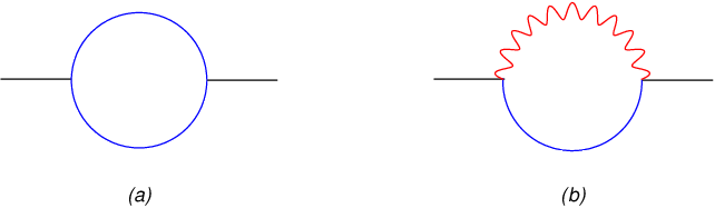
From (100) and (101), the wave function renormalization constant for the matter superfield is evaluated at one loop as
| (103) |
and the corresponding anomalous dimension (or gamma function) is immediately computed (in the limit ) as
| (104) | |||||
| (105) |
where superscript denotes -loop order. Replacing in (101) by , we get nothing involved either in or in . Here we assume that . That is, supersymmetry is not spontaneously broken in the visible sector. As a consequence, there is no one-loop contribution to the superconformal anomaly associated with the matter kinetic term.
Next, we inspect the two-loop contribution to the superconformal anomaly. First, the two-loop one-particle irreducible (1PI) supergraphs contributing to the propagator are shown in fig. 6, where a red blob denotes the relevant one-loop 1PI supergraph including any one-loop counter term that may be required [26]. Rather than directly calculate the two-loop 1PI supergraphs, we simply quote the result from the ref. [26, 27]. The infinite part of the two-loop contribution to the two-point function is [28]
| (106) | |||||
where we consider the general case with a semi-simple gauge groups with ’s being simple subgroups, and being the gauge coupling.

Comparing eq. (106) with the two-loop integral eq. (3.14) in ref. [29], we immediately find (see eq. (2.11) in ref. [30] or eq. (25) in ref. [26].)
| (107) | |||||
which is the coefficient of the finite term proportional to . What we need in two-loop contribution is indeed the finite term proportional to . This is because is replaced by
| (108) |

Second, there are one-particle reducible supergraphs at two-loop, shown in fig. 7. Each blue blob shown in fig. 7 represents either of the one-loop supergraphs shown in fig. 5. They should also be included in the computation for superconformal anomaly, which is very clear from Appendix C where the one-loop one-particle reducible vertex supergraphs make contributions to the superconformal anomaly but the one-loop 1PI vertex supergraphs do not. From eq. (101) and (105), we easily find that the coefficient of the finite term proprotional to is
| (109) |
Adding eq. (107) and (109) together we get the full expression proprotional to . This fact is clear from the relation, up to two-loop order,
| (110) |
with
| (111) | |||||
| (112) |
which agrees with the previous results computed using spurion method [6]. Eventually the LASM is given as
| (113) |
References
- [1] S. Ferrara and B. Zumino, Nucl. Phys. B 87 (1975) 207.
- [2] L. Randall and R. Sundrum, Nucl. Phys. B 557, 79 (1999) [arXiv:hep-th/9810155].
- [3] G. F. Giudice, M. A. Luty, H. Murayama and R. Rattazzi, JHEP 9812 (1998) 027 [arXiv:hep-ph/9810442].
- [4] E. Cremmer, S. Ferrara, L. Girardello and A. Van Proeyen, Phys. Lett. B 116 (1982) 231.
- [5] E. Cremmer, S. Ferrara, L. Girardello and A. Van Proeyen, Nucl. Phys. B 212 (1983) 413.
- [6] A. Pomarol and R. Rattazzi, JHEP 9905 (1999) 013 [arXiv:hep-ph/9903448].
- [7] M. F. Sohnius and P. C. West, Phys. Lett. B 105 (1981) 353.
- [8] V. P. Akulov, D. V. Volkov and V. A. Soroka, Theor. Math. Phys. 31 (1977) 285 [Teor. Mat. Fiz. 31 (1977) 12].
- [9] P. West, Introduction to supersymmetry and supergravity (1990), World Scientific.
- [10] M. Kaku, P. K. Townsend and P. van Nieuwenhuizen, Phys. Rev. D 17 (1978) 3179.
- [11] J. Wess and J. Bagger, Supersymmetry and Supergravity (1992), Princeton University Press.
- [12] T. E. Clark, O. Piguet and K. Sibold, Nucl. Phys. B 143 (1978) 445.
- [13] N. Arkani-Hamed and H. Murayama, JHEP 0006 (2000) 030 [arXiv:hep-th/9707133].
- [14] S. Ferrara and P. van Nieuwenhuizen, Phys. Lett. B 74 (1978) 333.
- [15] K. S. Stelle and P. C. West, Phys. Lett. B 74 (1978) 330.
- [16] S. Ferrara, L. Girardello, T. Kugo and A. Van Proeyen, Nucl. Phys. B 223 (1983) 191.
- [17] in preparation.
- [18] B. de Wit and M. Rocek, Phys. Lett. B 109 (1982) 439.
- [19] W. Siegel, Phys. Lett. B 85 (1979) 333.
- [20] M. T. Grisaru and P. C. West, Nucl. Phys. B 254 (1985) 249.
- [21] M. T. Grisaru, B. Milewski and D. Zanon, Nucl. Phys. B 266 (1986) 589.
- [22] Peskin, M. E. Peskin, D. V. Schroeder, Introduction to Quantum Field Theory (1994), Perseus Publishing
- [23] K. Fujikawa, Phys. Rev. Lett. 42 (1979) 1195.
- [24] M. T. Grisaru, W. Siegel and M. Rocek, Nucl. Phys. B 159 (1979) 429.
- [25] N. Arkani-Hamed, G. F. Giudice, M. A. Luty and R. Rattazzi, Phys. Rev. D 58 (1998) 115005 [arXiv:hep-ph/9803290].
- [26] P. C. West, Phys. Lett. B 137 (1984) 371.
- [27] D. R. T. Jones and L. Mezincescu, Phys. Lett. B 136 (1984) 242.
- [28] Y. Yamada, Phys. Rev. D 50 (1994) 3537 [arXiv:hep-ph/9401241].
- [29] L. F. Abbott and M. T. Grisaru, Nucl. Phys. B 169 (1980) 415.
- [30] S. P. Martin and M. T. Vaughn, Phys. Rev. D 50 (1994) 2282 [Erratum-ibid. D 78 (2008) 039903] [arXiv:hep-ph/9311340].