Proceedings of the Workshop
on Monte Carlo’s, Physics
and Simulations at the LHC
PART I
Authors
F. Ambroglini 19, R. Armillis 1, P. Azzi 20, G. Bagliesi 23, A. Ballestrero 4, G. Balossini 13, A. Banfi 5, P. Bartalini 26, D. Benedetti 35, G. Bevilacqua 30, S. Bolognesi 3, A. Cafarella , C.M. Carloni Calame 33, L. Carminati 6, M. Cobal 27, G. Corcella , C. Corianò 1, A. Dainese 29, V. Del Duca 41, F. Fabbri 9, M. Fabbrichesi 15, L. Fanò 16, Alon E. Faraggi 31, S. Frixione , L. Garbini 19, A. Giammanco 36, M. Guzzi 1, N. Irges 25, E. Maina 3, C. Mariotti 4, G. Masetti 8, B. Mele 12, E. Migliore 3, G. Montagna 13, M. Monteno 4, M. Moretti 18, P. Nason 10, O. Nicrosini 14, A. Nisati 12, A. Perrotta 9, F. Piccinini 14, G. Polesello 14, D. Rebuzzi 14, A. Rizzi 37, S. Rolli 42, C. Roda 23, S. Rosati 12, A. Santocchia 19, D. Stocco , F. Tartarelli 6, R. Tenchini 23, A. Tonero 17, M. Treccani , D. Treleani 7, A. Tricoli 38, D. Trocino 3, L. Vecchi 17, A. Vicini 6, I. Vivarelli 23.
- 1.
University of Salento and INFN, Lecce, Italy
- 2.
INFN, Frascati, Italy
- 3.
University of Torino and INFN, Torino, Italy
- 4.
INFN, Sezione di Torino, Torino, Italy
- 5.
University of Milano Bicocca and Sezione INFN, Milano, Italy
- 6.
University of Milano and Sezione INFN, Milano, Italy
- 7.
University of Trieste and Sezione INFN, Trieste, Italy
- 8.
University of Bologna and Sezione INFN, Bologna, Italy
- 9.
INFN, Sezione di Bologna, Bologna, Italy
- 10.
INFN, Sezione di Milano Bicocca, Milano, Italy
- 11.
INFN, Sezione di Milano, Milano, Italy
- 12.
INFN, Sezione di Roma, Roma, Italy
- 13.
University of Pavia and INFN, Pavia, Italy
- 14.
INFN, Sezione di Pavia, Pavia, Italy
- 15.
INFN, Sezione di Trieste, Trieste, Italy
- 16.
INFN, Sezione di Perugia, Perugia, Italy
- 17.
SISSA/ISAS, Trieste, Italy
- 18.
University of Ferrara and INFN, Ferrara, Italy
- 19.
University of Perugia and INFN, Perugia, Italy
- 20.
INFN, Sezione di Padova, Padova, Italy
- 21.
University of Padova and INFN, Padova, Italy
- 22.
University of Pisa and INFN, Pisa, Italy
- 23.
INFN, Sezione di Pisa, Pisa, Italy
- 24.
Scuola Normale Superiore and INFN, Pisa, Italy
- 25.
Department of Physics and Institute of Plasma Physics, University of Crete, Heraklion, Greece
- 26.
University of Florida, Gainesville, Florida, USA
- 27.
INFN Gruppo Collegato di Udine, Udine, Italy
- 28.
Museo Storico della Fisica e Centro Studi e Ricerche E. Fermi, Roma, Italy
- 29.
INFN, Laboratori Nazionali di Legnaro, Padova, Italy
- 30.
Institute of Nuclear Physics, NCSR “Demokritos”, Athens, Greece
- 31.
Department of Mathematical Sciences, University of Liverpool, Liverpool, United Kingdom
- 32.
Departamento de Física Teórica y del Cosmos, University of Granada, Granada, Spain
- 33.
INFN and School of Physics and Astronomy, University of Southampton, Highfield, Southampton, UK
- 34.
Subatech (Université de Nantes, Ecole des Mines and CNRS/IN2P3), Nantes, France
- 35.
Northeastern University, Department of Physics, Boston, MA, USA
- 36.
Université Catholique de Louvain, Louvain-la-Neuve, Belgium
- 37.
Institute for Particle Physics, ETH Zurich, Zurich, Switzerland
- 38.
Rutherford Appleton Laboratory, Science and Technology Facilities Council, Harwell Science and Innovation Campus, Didcot OX11 0QX, United Kingdom
- 39.
PH Department, TH Unit, CERN, Geneva, Switzerland
- 40.
ITPP, EPFL, Lausanne, Switzerland
- 41.
INFN, Laboratori Nazionali di Frascati, Frascati, Italy
- 42.
Tufts University, Medford, Massachusetts, USA
Preface
These proceedings collect the presentations given at the first three meetings of the “Workshop on Monte Carlo’s, Physics and Simulations at the LHC”, held on February 27-28, May 22-24 and October 23-25 2006 in Frascati (Italy). The purpose of the workshop, sponsored by the INFN, was to bring together all the complementary Italian scientific communities interested into high physics at the LHC. The workshop was thus attended by LHC experimental physicists, theoretical physicists dedicated to the calculation of matrix elements for collider processes and to the implementation of Monte Carlo programs, and theoretical physicists interested into model building and physics beyond the Standard Model. Theoretical Standard Model prediction, as well as physics signals from new models, are made available to the experimental community as Monte Carlo generators, that thus constitute the meeting points of the three communities mentioned above. The aim of the workshop was essentially to start to talk to each other, and to begin to understand the methods, the problems, and the language of the complementary communities.
Many of the presentations held at the first three workshop meetings were basic introductions to important theoretical and experimental topics relevant to LHC physics, and the speakers were requested to use a language suitable for people with no expertise in their field. The collection of these presentations constitutes thus an introduction to a few basic aspects of high LHC physics. It was decided to put them in the form of proceedings, maintaining the requirements of a language suitable for the complementary physics communities. In order to achieve this goal, the contributions were refereed internally, and have gone through several revisions. The second part of these proceedings collects more specialised presentations held at the workshop.
Although the very ambitious plan for these proceedings was not totally fulfilled (for instance, a few chapters were never completed), we feel that, at least for some of the chapters, we have met our goal. In particular, the first chapter constitute a very condensed presentation of the basics about LHC high physics, that can be used as a first introductory reading for the subject. The last chapter summarizes the basic features of the most important component of the ATLAS and CMS experiments, written in a way that should be easily understandable also by theorists. Many chapters of these proceedings11 1 together with the original slides of the presentations, available at http://moby.mib.infn.it/~nason/mcws/scientific_programme.htm. can be used for an introductory class on LHC high physics for graduate students in experimental and theoretical physics.
Although LHC physics is evolving rapidly, we believe that the basic argument treated in this volume will remain valid for an introduction, and that this effort will remain useful for the years to come.
Paolo Nason
Workshop’s Organizing Committee:
V. Del Duca,
B. Mele,
P. Nason,
G. Polesello (ATLAS),
R. Tenchini (CMS).
Workshop’s Conveners:
Shower Monte Carlo: S. Frixione, L. Fanó (CMS) S. Rolli (ATLAS);
Exact calculations at fixed order: F. Piccinini, P. Azzi (CMS);
SM and BSM Physics at LHC: B. Mele, M. Cobal (ATLAS), F. Fabbri (CMS);
Experimental Studies: F. Tartarelli (ATLAS), C. Mariotti, E. Migliore (CMS).
Introduction
Authors: Chiara Mariotti, Ernesto Migliore and Paolo Nason
Revisors: Sara Bolognesi
1.1 Physics at the Large Hadron Collider (LHC)
1.1.1 Introduction and basic references
In this chapter we give a very condensed summary of LHC physics. We assume that the reader has a basic familiarity with the Standard Model of electroweak and strong interactions. We summarize here some easily accessible basic references to introductory material. In ref. [1] an introduction to the Standard Electroweak theory can be found, together with a summary of precision tests, and hints on physics bejond the Standard Model. A very basic introduction to the theory of strong interaction can be found in refs. [2]. Summaries on the Electroweak and strong interaction, as well as on experimental methods, can be found in the reviews of the Particle Data Group, available at the URL http://pdg.lbl.gov.
1.1.2 Why LHC?
The Standard Model (SM) of electroweak interactions has been established experimentally by the observation of neutral current interactions in 1973 [3] and of the W and Z bosons in 1983 [4, 6]. From 1989 to 2000, the LEP and SLC experiments measured with a better than per-mill precision the properties of the W and Z bosons: their masses, their widths, their couplings with fermions and among themselves. These measurements were complemented by the Tevatron observation of the top quark. The piece of the SM which is still missing is the Higgs boson, which is a remnant of the scalars that provide masses to the particles. Actually, the same precision measurements of the electroweak observables hint to a light Higgs boson. In fact the accuracy reached requires that, when relating them among each other, genuine electroweak quantum corrections should be included, namely:
| (1.1) |
(see ref. [1])
where the quantum corrections have a quadratic dependence on the mass of the top
quark and a logarithmic dependence on the mass of the Higgs:
.
With , and being measured, can be
extracted from a global fit of the electroweak observables.
On the other hand the lower limit on the Higgs mass from direct searches is
currently 114.4 GeV at 95% confidence level. An upper limit on around 1.2 TeV is derived
within the SM requiring that the amplitude for the scattering of
longitudinally polarized vector bosons
does not violate unitarity.
The discovery of the mechanism which gives origin to the
masses requires the investigation of the energy range from 100 GeV to
1 TeV, and actually LHC has been designed as a discovery machine for processes with
cross-sections down to some tens of fb and in the energy range from 100
GeV to 1-2 TeV.
This physics goal influenced the main design parameters of the
machine:
- •
It is a hadron collider: the fundamental constituents entering in the scattering are the partons which carry a variable fraction of the beam four-momentum. Therefore the centre-of-mass energy of the hard scattering process can span different orders of magnitude.
- •
The centre-of-mass energy will be =14 TeV. In this way, incoming partons carrying momentum fractions of the incoming hadrons momenta, yield a partonic CM energy TeV, the energy range one wants to explore.
- •
It is a proton-proton collider since it is difficult to accumulate high intensity beam of anti-protons. Furthermore, the Higgs production process is dominated by gluon fusion, and therefore its cross section is nearly the same in proton-antiproton and proton-collision.
- •
The time interval between consecutive bunch crossing will be 25 ns, as the luminosity depends linearly on the bunch crossing frequency. The very short bunch crossing interval and the high number of bunches accelerated by the machine (2808 per beam) will allow to reach the peak luminosity of 1034 cm-2s-1.
With respect to an electron-positron machine, it is easier to accelerate protons to high energy since the energy lost for synchrotron radiation, proportional to (where ) is much lower than for the electrons. On the contrary precision measurements are more difficult. Since the kinematics of the initial state of the hard process can change from event to event, it is possible to have more than one fundamental interaction per bunch crossing, with the fragments of the protons mixing with the products of the hard process in the final state.
The luminosity delivered by LHC during the first 3 years will be of fb-1 per year or
cm-2s-1, and later
fb-1 per year or cm-2s-1.
Two general-purpose experiments are in construction: ATLAS (A Toroidal Lhc ApparatuS)
and CMS (Compact Muon Solenoid). A B-physics dedicated experiment (LHCb) is also
in preparation, and is dedicated to the study of b-hadrons produced at small angle
in p-p collisions at low luminosity. Finally, the LHC will also provide Pb-Pb collision
with TeV and a luminosity of cm-2s-1. The ALICE
experiment will be devoted to study these collisions.
1.1.3 The ATLAS and CMS physics program
The main goals of the two general purpose experiments are:
- •
study the mechanism that breaks the symmetry of the SM Lagrangian giving rise to the particle masses.
Whitin the SM this means to search for the SM Higgs boson from =100 GeV to =1 TeV. If the Higgs is found, understand if it is a SM Higgs or a SUSY Higgs; if the Higgs is not found, look for alternative models. - •
search for new physics, especially if the Higgs is not found.
Concerning supersimmetry, all the s-particles with mass 3 TeV will be accessible. For exotic models (lepto-quark, technicolor, new strong interaction, new lepton families, additional bosons, extra-dimensions …) the mass reach is 5 TeV. - •
perform precision measurements in the electroweak sector (, , triple gauge couplings, ), in QCD, and in the CP violation and B physics sector.
Concerning the precision electroweak measurements, it should be noted that, in order to have a comparable impact in the determination of the Higgs mass from the fit of the electroweak observables, the top mass and the W mass should be measured with a relative precision given by:Therefore the target precision on these quantities will be 15 MeV and 2 GeV. These precisions will not be trivial to achieve, since at a hadron collider the initial state of the parton-parton collision is not well known, and the final state is complicated by the presence of many other produced particles.
In figure 1.1 are shown some of the cross-sections (as a function of the centre-of-mass energy and the rate of production) of interesting processes. In table 1.1 we report the cross-section and the number of events produced per experiment for a given process, for low luminosity ( cm-2s-1).

| Process | Events/sec | Events/year | Other machine | |
|---|---|---|---|---|
| 20 nb | 15 | 108 | 104 LEP / 107 Tevatron | |
| 2 nb | 1.5 | 107 | 107 LEP | |
| 1 nb | 0.8 | 107 | 105 Tevatron | |
| 0.8 mb | 105 | 1012 | 108 Belle/BaBar | |
| (m = 1 TeV) | 1 pb | 0.001 | 104 | |
| H (m = 0.8 TeV) | 1 pb | 0.001 | 104 | |
| H (m = 0.2 TeV) | 20 pb | 0.01 | 105 |
1.2 The theory of Hadronic collisions
1.2.1 Hadron collider kinematics
A convenient set of kinematic variables for particles produced in hadronic collisions is the transverse momentum , the rapidity and the azymuthal angle . Assuming that the collision axis is the third axis, in the CM frame of the collision, for a particle with energy and three momentum we write
| (1.2) |
These variables have simple transformation properties under longitudinal boosts (i.e. boosts along the beam line direction), and being invariant, and
| (1.3) |
where is the boost velocity along the third direction. The energy and the longitudinal component of the momentum of a particle have the expression
| (1.4) |
where is the mass of the particle, and is called the transverse mass.22 2 In mass measurements at hadronic colliders the term “ transverse mass” is used to denote the observable , and has a totally different meaning from the one introduced here. One usually refers to the regions , and as to the forward, backward and central region.
Observe that the single particle invariant phase space is written in terms of rapidity and transverse momentum as
| (1.5) |
and is thus flat in rapidity. Furthermore, the cross section for the production of an object of mass , for not too extreme values of the mass and rapidity, is typically flat in rapidity. This can be seen as follows. The production cross section is proportional to
| (1.6) |
where are the parton densities and are the momentum fraction of the incoming partons. The rapidity of the produced particle is given by . Defining one can easily show that
| (1.7) |
Assuming33 3 This is the typical small- behaviour of parton densities, with . that , we see that formula (1.6) yields a flat rapidity distribution. This of course holds as long as the rapidity is not close to its maximum value . Thus the typical rapidity distribution has a bell shape with a central plateau, the plateau becoming wider as becomes small.
The use of boost invariant variables facilitates the description of particle production in hadronic collisions, since these phenomena are approximately boost invariant for not too extreme values of rapidity. This fact is particularly simple to understand for high energy scattering phenomena, where the incoming hadrons behave as beams of quark and gluons, with a given distribution in longitudinal momenta and limited transverse momentum. It is clear that, depending upon the energy of the incoming constituents, the same hard scattering phenomenon can take place with an effective center of mass (i.e. with a center of mass for the incoming constituents) that is moving along the collision direction.
Experimentally, it is more convenient to use the pseudorapidity, rather than the rapidity. It is defined as
| (1.8) |
where is the angle of with respect to the positive 3 direction. Being only a function of the angle, pseudorapidity is much easier to measure than rapidity, and for ultrarelativistic particles it coincides with rapidity. The analogue of eqs. (1.4) for pseudorapidity are
| (1.9) |
The particles distribution in hadronic collisions are often represented as a 3-dimensional histogram on a rectangle in the , plane (the range in being dependent upon the detector’s capability) obtained by cutting the , cylinder surrounding the colliding beams, and centered at the collision point, along the line. On this plane, one also defines a distance .
1.2.2 Orders of magnitude
The total cross section for proton-proton collisions is in the range of few tens of millibarns (). This is consistent with a transverse size of a hadron of the order of a femtometer (), a being equal to 10 mb. The cross section grows slowly with energy, so that projected values at LHC energies are around 100 mb, as one can see from fig. 1.2.
The total inelastic cross section is mainly made up of events with low hadrons in the final state.44 4 These events are often called minimum bias events. The term originates from the so called minimum bias trigger selection, that was the trigger using the less stringent criteria, thus yielding the least biased event sample. In older experiments, these events had typically some particles in the central region. Today, more detailed definitions are used, and we refer the reader to sec. Minimum Bias, Underlying Events and Multiple Interactions for further discussion. These events are sometimes classified according to the distributions of the produced particles in the available rapidity (or pseudorapidity) interval. If there are empty gaps, inelastic events are classified as diffractive events, as shown in fig. 1.3. The value of their measured cross section at Tevatron energy, and their extrapolated cross section al LHC energy is also shown in the figure.
Most of the total cross section is composed by events with no evident gaps. They are characterized by transverse momenta of the produced particles of the order of few hundred MeV, and particle multiplicity (that is to say, number of produced particles) of order of a few per unit of rapidity, with fluctuations of the order of 100%. A more detailed description of typical inelastic events will be given in chapter Minimum Bias, Underlying Events and Multiple Interactions.
An extrapolation of the average number of charged particles per unit of pseudorapidity to LHC energy is shown in fig. 1.4.
Observe that the distributions in fig. 1.4 have a dip at . This is a kinematical effect, due to the use of pseudorapidity instead of rapidity. Rapidity distributions would instead be flat in the small rapidity region, thus showing the boost invariant feature of particle production in hadronic collisions.55 5 From eqs. (1.4,1.9), we have , showing that, when mass effects are not negligible, for small pseudorapidity intervals are wider than the corresponding rapidity intervals.
The main purpose of high energy colliders is to study scattering phenomena with very large momentum transfer, or production processes of very massive, pointlike particles. These processes are collectively called “hard scattering” phenomena. In these cases, incoming hadrons can be regarded as beams of pointlike constituents. The cross sections for constituents hard scattering are much smaller than the total hadronic cross section. They are of the order of the squared inverse of the typical energy scale entering the process, sometimes called the hardness of the process, times a dimensionless coupling constant. Thus, for example, the cross section for production is of order66 6 The notation stands for the running QCD coupling constant at the scale . , corresponding to about GeV-2 or mb. This is to be compared with the 100 mb cross section for a typical low transverse momentum reaction, the ratio being . We notice that an estimate of the cross section for jet production is given by , where is the transverse momentum of the jet. For of the order of few hundreds MeV, the strong coupling becomes of order one, and thus this cross section becomes of the same order of the typical low transverse momentum reactions.
1.3 QCD description of hadronic collisions
1.3.1 Hard production processes
Inclusive cross sections for hard production processes are calculable in terms of the so called QCD-improved parton model formula
| (1.10) |
Here represents the cross section for some hard phenomenon to take place (for example, the production of some heavy particle, eventually with some kinematics constraints, the production of jets with a large transverse momentum, etc.). The labels and run over all quarks, antiquarks, and the gluon. The parton densities represent the probability to find the constituent inside the hadron , carrying a fraction of its momentum. The scale must be chosen to be of the order of the typical hard scale entering the process (like, for example, the mass of the in production, the transverse momentum of the jet in jet production, etc.). The so called “short distance” or “partonic” cross section is calculable in perturbation theory as an espansion in powers of the strong coupling constant , evaluated at a scale also of the order of the typical hard scale entering the process.
Formula (1.10) cannot be used to predict the detailed distribution of all final state particles. It must instead refer to a sum of final states, that is to say it must be inclusive to some degree. First of all, the formula does not say anything about the fate of the remnants of the incoming hadrons after the collisions. Beside this, certain characteristics of infrared insensitivity should be requested to the cross section in order for it to be calculable in QCD. In other words, our cross section should not depend upon the infrared cutoffs that we use in our calculation. In general, the differential production cross sections for heavy particles satisfy these requirements. Not so for massless coloured particle production. High transverse momenta coloured partons in the final state materialize as jets, that is to say as sprays of relatively collimated particles. Rather than the kinematical distribution of final state particles, it is the jet kinematics that is calculable. Thus, the cross section must be inclusive also in the composition of a jet, in that it must include all final states that have the same jet structure. Finally, one cannot forbid QCD radiation in any angular region of phase space, in order for the cross section to be calculable, that is to say, as in QED, one must require a minimal energy resolution of the measuring apparatus in order to obtain sensible results. This last point is basically related to the requirement of cancellation of soft divergences.
To better clarify the meaning of formula (1.10) and the origin of its limitations, we will now consider the example of production in hadronic collisions, depicted in fig. 1.5.
The diagram (a) represents the Born level cross sections, while (b) and (c) are next-to-leading order (NLO from now on) contributions. The Born result represents the cross section for the production of a with given kinematic properties, plus anything else. The next-to-leading contributions (b) and (c) represent corrections to (a) that are formally of order , but receive large contributions in particular regions of phase space. In particular, if the outgoing gluon momentum is parallel to one of the incoming quarks.
1.3.2 Collinear singularities
Let us briefly review what happens when a gluon is emitted collinearly by an initial state parton (like the incoming quark in our example). In lowest order perturbation theory, the emission cross section factorizes as
| (1.11) |
where is the gluon momentum, and we have assumed , i.e. we have decomposed the gluon momentum into a component parallel to the initial state parton , and a component orthogonal to it, . The collinear limit is reached when , so that the direction of the incoming quark and of the emitted gluon coincide. The cross section becomes the product of the production cross section with a reduced momentum for the incoming quark, times a splitting probability, proportional to the strong coupling constant evaluated at the characteristic transverse momentum of the splitting process. is the Altarelli-Parisi splitting function for finding a gluon in a quark with a fraction of its momentum
| (1.12) |
and it describes the distribution of the splitting probability as a function of the fraction of longitudinal momentum. Of course, formula (1.11) makes no sense for too near ( becomes too large and perturbation theory can no longer be applied), and for of order (factorization only works for small ). We can however use it to estimate the order of magnitude of the probability for the emission of an extra gluon. Using the one loop formula for the strong coupling constant
| (1.13) |
we can estimate the size of the contribution of one extra collinear emission in formula (1.11) by performing the integration
| (1.14) |
Assuming that and of the order of the transverse mass of the , we see that the right hand side of eq. (1.14) is not small, i.e. is not suppressed by a power of the strong coupling at the hard scale. However, most of the contribution to the integral take place at low , as can be seen from fig. 1.6, so that the probability to emit a hard gluon is indeed of order .
This reasoning can be extended for the emission for any number of gluons, with . We would find that also multiple emissions have probability of order 1. The presence of these large contributions due to collinear parton emissions are among the reasons why the detailed final state structure is not described by formula (1.10). In fact, the sum of all these large corrections (and of the associated large corrections present in the virtual contribution of fig 1.5 ) is already included in eq. (1.10), since the scale dependent parton densities include the effect of all emissions with up to . Thus, if , the only left over corrections in eq. (1.10) are genuine strong radiative corrections, suppressed by powers of . We must however assume that we sum over all final state configurations that have any number of collinear partons in the direction of the incoming quark or antiquark.
In processes with a massless parton with large transverse momentum in the final state, one also expects large corrections due to radiation collinear to it. The factorization formula is similar to eq. (1.11). Consider the example of diagram (b) in fig 1.5, under the assumption that the final state gluon has large transverse momentum. The gluon can split into a pair of collinear gluons, with cross section
| (1.15) |
where now , and is transverse with respect to the direction of the outgoing gluon. One noticeable difference between eq. (1.15) and eq. (1.11) is that in the former case gluon radiation reduces the momentum entering in the hard cross section. For final state splitting, instead, the momenta flowing through the hard scattering process are unchanged. These large final state radiation corrections, in fact, cancel out when virtual corrections are included. Virtual corrections do not change the structure of the final state, since they correspond to the emission and reabsorption of a virtual parton. Thus, the cancellation works only if one is allowed to sum contributions with different final state structure. In other words, rather than requiring a given light parton in the final state, we should require the presence of a jet, that is to say of a bunch of collimated particles.
1.3.3 Soft singularities
Soft gluon emission also gives rise to divergencies of the form , where is the gluon energy. These divergences are present whenever coloured particles are involved in a reaction, and are analogous to the soft divergences in electrodynamics. In electrodynamics, soft singularities are a basic consequence of quantization. In fact, the brehmmstralung frequency spectrum is known to approach a constant for small frequencies. Because of quantization, , so that, if is a constant, , that is to say it diverges at low frequencies. Because of this fact, QED radiative corrections have always infrared divergences related to (both real and virtual) emission of soft photons. It turns out, however, that if one assumes that there is a finite energy resolution for soft photons (i.e., that one cannot detect photons with energy below a given cut ), soft divergences between real and virtual corrections cancel out, yielding a finite result. The same thing happens in QCD. Because of this virtual-real infrared cancellation, it also turns out that we cannot totally veto radiation in any angular region of the phase space. This veto would affect the soft gluon emission contribution to the cross section, but would leave the corresponding virtual correction unchanged, thus spoiling the cancellation.
If massless coloured particles are present in a reaction, collinear and soft singularities are present at the same time. In particular, in formula (1.11), since , we see that the integration yields a integral, that corresponds (when is already small) to the gluon energy becoming small. The region where a gluon becomes both collinear and soft is sometimes referred to as the double logarithmic region, because of the presence of two factorized logarithmic singularities.
1.3.4 Jet definitions
We have seen that we cannot predict the distribution of individual massless partons in the final state, but we should instead talk about jets. There is much freedom in the way jets are defined. In order for a jet cross section to be calculable in perturbation theory, it should be insensitive to the splitting of a massless particle into two collinear partons, in such a way that the cancellation between real and virtual contributions to the cross section can take place. A typical jet definition may deal with the total amount of energy flowing from the interaction vertex into a cone of fixed aperture. A jet definition must be collinear insensitive in order to be calculable in perturbation theory. This is however not enough. We cannot characterize the final state by requiring that all final state particles lie inside cones of given aperture. In fact, because of soft divergences, we cannot require that there are regions in solid angle where there are no particles at all. This requirement would spoil the cancellation of infrared divergences. We should thus allow a limited fraction of the total energy to be present in arbitrary directions outside the cones (the so called Sterman-Weinberg jet definition), or we should instead deal with inclusive jet cross section, meaning of a given number of jets above a given energy plus an arbitrary number of jets of smaller energy.
1.3.5 Fixed order calculations
The QCD improved parton model formula, eq (1.10), applied at any given finite order in the strong coupling constant, can be used to compute certain cross sections, i.e. inclusive cross section for the production of heavy particles and/or jets. For these quantities, soft singularities cancel (and so do the collinear final state singularities) between real and virtual contributions. Initial state collinear singularities survive, but are subtracted and absorbed into the scale dependent parton densities. At the Born level, one only considers the cross section for the production of a given number of heavy particles, and of well separated massless partons. At this level, one associates a jet to each massless parton. At the NLO level, corrections due to the virtual exchange of a massless parton, or to its emission, are included. At this level, it is possible to have jets containing more than one massless parton, since the radiated particle can be collinear to any other massless parton in the process. The emitted parton can be soft, and their emission cross section diverges in the soft limit. These divergences cancel among real and virtual graphs. Fixed order calculations are the backbone of our theoretical ability to predict hard scattering cross sections. Automatic algorithms exist that allow one to compute arbitrary Born level cross sections, the only limitation being the computer time for very complex processes. For many processes of interest, the NLO corrections have also been computed, within a framework to deal with collinear and soft singularities in a consistent way. Since a few years, some results at NNLO level have also become available.
1.3.6 Shower Monte Carlo
From the discussion carried out so far, it is clear that the QCD parton model formula alone does not fully describe the final state in hadronic collisions. First of all, we lack a practical way of computing QCD at low energy, and thus we are incapable to describe the formation of a final state made up of hadrons. But, even if we put aside this problem, we have seen that the formation of a specific final state involves an arbitrary number of collinear (and soft) emissions, all of them contributing corrections of order one. These corrections cancel for inclusive observables. Sadly, a specific final state is not inclusive by definition, and so fixed order calculations cannot predict its probability. There are, however, algorithms that are capable to resum to all order in perturbation theory all most important real and virtual emission corrections (namely the corrections that are collinear divergent), the so called shower algorithms. These algorithms are thus capable to associate with a given hard event an arbitrary number of accompaning partons. In order to yield a finite result, they must contain an explicit cut-off on the transverse momentum of emitted partons, and on their energy. The final state they generate is still unphysical, since it is made up by quarks and gluons, rather than hadrons. In order to generate a physical final state, phenomenological models of hadron formation are used. These models are not soundly motivated from a theoretical viewpoint. However, it is also true that the same models should be applicable to any hard collision, since the part of the collision that involves distances below the typical hadronic scale is well described by the perturbative QCD formalism embodied in the computation of the short distance cross section and of the shower development. Shower Monte Carlo programs are thus event generators that can model the full final state. They have been successfully employed in several experimental frameworks, like electron-positron, lepton-hadron, and hadron-hadron collisions, at several different energies. We expect that they should work with some tuning also for LHC.
Underlying event
The QCD picture of an event, as represented by a shower Monte Carlo and a hadronization model, still misses one ingredient for the description of the full final state. In fact, at the end of the shower, the system is represented by two incoming partons and a number of final state partons. Given that the fragmentation process turns final state partons into real hadrons, we still have to specify how to treat the remnant of the two initial hadrons that have provided the initial state partons. These remnants carry energy, momentum, flavour and colour, so their treatment is indispensable for a realistic description of the event. We are unable, at present, to describe this aspect of the process within QCD, and thus we have to resort to a model, the so called “Underlying event model”. One very crude model would be to include the hadron remnant in the final state (for example, if the incoming parton is a quark, the hadron remnant is a di-quark), and provide a mechanism for the hadronization of the remnant (that will be typically correlated in colour to some final state partons) in the fragmentation stage of the shower.
The name “Underlying event” is somewhat unfortunate, since it gives the false impression that there is some uncorrelated activity accompaning any hard scattering process. It is also used with some ambiguity in the literature. In fact, there is no precise way to separate the underlying event from the hard process. In the framework of the Event Generators, the underlying event model (in general made up of several components) describes the physics of the hadronic remnants. When fitting the parameters of these components, one typically looks at regions of phase space where the influence of the hard process is as small as possible, like for example angular regions in the azimuth that are as far as possible from the jets in jet pair production. In case of production of colour neutral particles, like the or the , after the removal of the or decay products from the final state, the distribution of all remaining particles should be strongly dependent upon the “Underlying event” model.
Multiple parton interactions
The physics of the hadron remnants may influence in several ways the formation of the final state, and not only in the very forward direction. First of all, the remnants are coloured, and thus can radiate soft gluons. They can also give rise to secondary parton interactions. Thus, for example, in our production process, another pair of constituents from the incoming hadron can collide, and generate two balanced jets that accompany the , or they can even produce another .
The probability for a secondary interaction can be easily estimated. Since a hard scattering has taken place, this means that the two hadrons have overlapped in the transverse plane, with an overlapping area of the order of . An estimate of the probability for another hard cross section is given by the ratio of the hard cross section divided by the transverse area of the overlapping region. In the case of the production of an extra pair of jets with transverse momentum , the probability is
| (1.16) |
It is thus a power suppressed effect. The perturbative description of the collision we have introduced so far deals with effects that are at most suppressed by powers of the coupling constant, not by powers of the strong interaction scale. Nevertheless, for relatively small , multiparton interactions can be important for a full description of the event. Modern underlying event models do include secondary interactions, as discussed in Minimum Bias, Underlying Events and Multiple Interactions.
1.4 The detectors
This section is meant to be an introduction to the experimental aspects of the investigation of high energy proton-proton events. The outline of the section is the following:
- •
review the basic physics processes involved in the detection of particles in the energy regime typical of LHC;
- •
describe how different detection systems can be gathered into general purpose apparatus to provide the most exhaustive picture of each proton-proton collision;
- •
a short description of how these different components have been implemented in the ATLAS and in the CMS experiments.
Deeper discussion of physics objects, trigger, simulation will be done to Chapter/Session 4.
1.4.1 Basics of particle detection
Experimentally the measurement of a particle is the determination of its four-momentum and the identification of its type, namely mass and charge. Modern particle detectors are based on the conversion of an absorbed energy into an electrical signal. The processes leading to the formation of the signal depend on the particle type and energy. Considering only the energy range typical of particles produced in high energy collisions, i.e. from several hundreds MeV to several hundreds GeV, and the particles whose lifetimes are long enough to reach the detectors, i.e. cm, the main processes are:
- •
electrons/positrons: the energy loss is determined by ionization and bremsstrahlung processes the latter being dominant from the energy at which they are produced down to a critical energy whose typical value is of the order of ten(s) MeV.
- •
muons: the energy loss is determined by ionization and bremsstrahlung processes. As the dependence of the bremsstrahlung energy loss per unit length on the particle energy and mass goes as , the bremsstrahlung process for the muons starts to be relevant at hundreds GeV. As they do not interact strongly and as the probability of showering 77 7 See below for a description of a shower process. is small, they can penetrate deeply in the material, as Minimum Ionizing Particle (MIP).
- •
charged hadrons (essentially and protons): the energy loss is determined by ionization and strong interactions with the nuclei of the material.
- •
neutral hadrons (essentially and neutrons): the energy loss is determined by strong interactions with the nuclei of the material. It should be noted that neutral pions quickly decay electromagnetically (=25 nm) before having a chance of re-interacting hadronically.
- •
photons: the energy loss is determined essentially by pair production for energies above some MeV. The electron and positron produced behave as described above.
As the main interaction mechanisms of high energy electrons (i.e. Coulomb scattering and bremsstrahlung) and of high energy photons (i.e. pair production) are described by closely related diagrams they all can be characterized by the same parameter: the radiation length , which expresses the mean distance over which a high-energy electron loses all but of its energy by bremsstrahlung or equivalently of the mean free path for pair production by a high-energy photon.
All the charged particles interacts by elastic Coulomb scattering at low momentum transfer off the nuclei of the medium thus resulting in a change of direction which affects the direction of (Multiple Scattering). The distribution of initially collimated unit charge particles emerging from a slab of material of thickness and radiation length has a Gaussian core with a spread projected into a plane with non-gaussian tails generated by the collisions at large momentum transfer.88 8 A very rough explanation of this formula is as follows. Coulomb scattering and bremsstrahlung effects are related, since Coulomb scattering is the cause of bremsstrahlung. Thus the number and intensity of random transverse kicks is proportional to , and the variance in the total transverse kick goes like . The accounts for the fact that slower particles spend more time in traversing the atoms they collide with, and the kick in momentum is proportional to the product of force and time. The factor translates a transverse momentum kick into an angle.
1.4.2 Measurement of the four-momentum: spectrometers and calorimeters
Spectrometers.
Spectrometers determine the three-momentum of a charged particle from observing how it bends in a magnetic field. A unit charge particle crossing a uniform magnetic field with momentum in the plane perpendicular to the direction for a region of length deflects from the straight line of a sagitta (see figure 1.8):
| (1.17) |
with in T, in m and in GeV.
From and from the knowledge of the trajectory
(i.e. the angle between the track and the field directions)
the three-momentum is determined as .
If no particle identification is available, the energy of the particle
is then computed assuming the mass of the charged pion which is the most
abundant charged particle in the event.
The resolution on is related to the geometric accuracy on the
measurement of the sagitta by
| (1.18) |
To achieve observable bendings, in collider experiments magnetic
fields of several Teslas are used (2 T in the ATLAS and 4 T in the CMS
solenoids respectively).
For example the sagitta of a particle with =1 TeV crossing a 1 m long region with a 4 T
field is about 150 m. Thus a 10% measurement of the momentum
requires an accuracy on the sagitta of 15 m.
As the geometrical accuracy on the sagitta does not depend
on , decreases for
increasing values.
Multiple scattering mimics the magnetic field deflection thus
affecting the resolution by a factor which does not depend on .
The actual effect on the resolution depends on whether the measurament
of the trajectory is performed in a homogeneous volume (figure
1.8 left), as in the case of Time Projection Chambers,
or in an air-gap spectrometer with the track measured by discrete
tracking planes (figure 1.8 right), as in the case of
silicon strip tracking detectors.
In the case of the homogeneous volume the determination of the sagitta
is mainly affected by the lateral dispersion, , leading to:
| (1.19) |
In case of air-gap spectrometer the dominant contribution is the kink experienced by the particle when crossing a measurement plane of thickness :
| (1.20) |
The trajectory of the charged particle is measured by tracking detectors (cf. Sect. 1.4.3) which determine the points where the particle crossed their sensitive volume. Because of the multiple scattering, tracking detectors ideally should be massless and with no passive material in front. The multiple scattering dominates at low values of , while at high values the geometrical term dominates.
Calorimeters
Calorimeters are detectors which measure the energy of a particle by means of total absorption of its energy. The process at the basis of the degradation of the energy of the incoming particle is the development of a shower. Two kinds of showers can be distinguished according to the nature of the incoming particle:
- •
electromagnetic showers.
The interaction of photons and electrons above 10 MeV is dominated by the processes:- –
pair-production
- –
bremsstrahlung
both characterized by the radiation length . On average after 1 a produces an pair while an radiates a bremsstrahlung photon, with the produced particles sharing the energy of the initial one. The cascade of these processes produces a so-called electromagnetic shower which evolves with the number of particles increasing at each step while their energy is decreasing. Below a certain threshold the process stops with a number of particles in the shower related to the energy of the initial particle. The depth at which the shower stops grows logarithmically with the initial energy of the incoming particle. 99 9 Assuming that at each branching the energy equally splits among the decay products, the length for a full containment of a shower developed by an incoming particle of energy is The typical depth of an electromagnetic calorimeters in a high energy physics experiment is about 27 . The energy of an electron/photon is then obtained from counting the charged particles which are in the shower, actually measuring the energy deposited by them, and applying some calibration function which has been determined previously in conditions where the energy of the incoming particle was known, as in test-beam or in-situ, i.e. in the experiment itself using events where the energy is well known for example by kinematic constraints of the event. The determination of the energy with a calorimeter is a stochastic process (the measured quantity is the signal released by particles with ) and therefore its resolution improves with increasing energy 1010 10 The notation indicates the sum in quadrature.
(1.21) The first term is referred to as the noise term (signal fluctuations independent from the shower energy, typically electronics read-out noise), the second as the stochastic term (statistics fluctuations in the various processes from the shower development up to the signal formation), the last as the constant term (typically due to detector inhomogeneities).
Multiple scattering of produces a broadening of the shower also in the transverse direction which is characterized by the Moliere radius : 95% of the energy of the shower is contained within a cylinder of radius . - –
- •
Hadronic showers: if the incoming particle is a hadron, the showering process is dominated by a sequence of inelastic hadronic interactions. At high energy, these are characterized by multi-particle production and particle emission originating from nuclear decay of excited nuclei. The principle of the energy measurement is the same as for the electromagnetic case: counting the number of charged particles in the shower and converting it into an energy value by means of a known calibration function. Similar considerations for the energy resolution holds as for the case of electromagnetic calorimeters, but the energy resolution is worse than that of electromagnetic calorimeters essentially because of three effects:
- 1.
part of the energy goes into excitation of break-up nuclei without being detected;
- 2.
on average 1/3 of the pions produced (i.e. the lightest hadron) are which immediately decays electromagnetically giving a larger signal than a charged pion of the same energy;
- 3.
hadrons can decay in final state with a neutrino (undetected) or a muon (small signal).
The typical scale of the process is the nuclear interaction length which for materials heavier than iron is one order of magnitude larger than the electromagnetic interaction length . For this reason hadronic calorimeters are longer and placed besides electromagnetic calorimeters.
- 1.
Technically two types of calorimeters exists: homogeneous calorimeters where the same material acts as the medium where shower develops (absorber) and signal is produced (detector) and sampling calorimeters (absorber material different from detector material). Typical examples of homogeneous calorimeters are high-Z material crystals while for sampling calorimeters are sandwiches of high-Z materials and gas or liquid detectors or plastic scintillators. In the detector material the produced ionization or the scintillation light emitted in the de-excitation of the crystal lattice for inorganic scintillators (or of vibrational modes for organic ones) is collected. Hadronic calorimeters are usually sampling calorimeters.
The determination of the direction of the incoming particle with a calorimeter is achieved by means of a segmentation of calorimeter into cells read-out separately. In case of an electromagnetic shower the three-momentum is then just computed assuming a massless kinematics, i.e. the measured energy as the absolute value of the momentum and the same direction for and the shower.
1.4.3 Measurement of the topology of the event: vertex and tracking detectors
Because of their fast response, the LHC tracking systems are mainly based on finely segmented solid-state detectors: two or three shells of 2D pixel detectors close to the interaction point at 10 cm with a typical pixel size of 150x150 m2, followed by 4 shells of 1D strip detectors at 2050 cm with a typical pitch distance between neighboring strips of about 100 m. This layout is dictated by the requirement of keeping the fraction of hit channels of the detectors per LHC bunch crossing, called occupancy, at a level of 1-2% thus keeping at an affordable level the combinatorics that the track finding algorithms have to deal with.1111 11 At =14 TeV and at cm-2s-1 there are about 1000 tracks per bunch crossing which, in absence of magnetic field, would be distributed as . The magnetic field actually confines charged particle and the actual distribution is more (less) pronounced than the at lower (higher) radii. The position of the measured point is provided by the channel fired by the passing charged particle. Therefore the resolution (for a single coordinate) is basically the width of the read-out cell divided by that for the geometry described above is typically of about 30 m (a 3D point is reconstructed by the pixel detectors while a 2D point is typically reconstructed by the strip detectors: the extra coordinate is given by the position of the detector itself.) Accurate measurements of the particle tracks close to their production point can be exploited for:
- •
reconstruct the primary vertex of the event. At high luminosity there will be on average 20 inelastic proton-proton collisions at each bunch-crossing: grouping all particles coming from the same primary vertex is an essential simplification for the analysis of the LHC events;
- •
identify long-lived particles (typically hadrons containing a heavy quark) which travel up to few mm before decaying. They can be identified as their decay (secondary) vertex is displaced by their production (primary) vertex. This identification (tagging) is based on the fact that the impact parameter of the daughter particles produced at the decay vertex, i.e. the distance of minimum approach of daughter tracks to the primary vertex, is significantly different from zero. The impact parameter is larger than the one of particles coming from the interaction vertex, because of the large mass of the long living hadron (thus the relatively high of the decay products with respect to the hadron flight direction) and because the tracks come from a secondary vertex that is produced few millimeters away from the primary one.
The resolution on the impact parameter depends on the geometrical resolution of the detector and on the multiple scattering:
| (1.22) |
The geometrical resolution depends on the layout of the detector, namely the intrinsic resolution of the sensing element (i.e. the pitch of the strips or the dimension of the pixels, typically m), the distance from the primary vertex of the layer of the detector that gives the first measurement of the track, and on the total lever arm of the vertex-detector:
| (1.23) |
The multiple scattering term is due to the presence of material along the particle trajectory and it depends on the momentum of the particle, on the amount of material crossed (which in turn, assuming a detector with cylindrical geometry, depends on the angle at which the particle is emitted, being the angle with respect to the beam direction):
| (1.24) |
Thus a performant detector must have the first layer as close as possible to the interaction region (i.e. as small as possible), limited by the dimension of the beam pipe, the lever arm as large as possible and the material as thin as possible in unit of . Moreover the detector should maximize the number of layers, in order to minimize the error and ambiguities in the pattern recognition during the reconstruction of the trajectory.
1.4.4 General purpose detectors
General purpose detectors are designed to measure as many as possible of the particles produced in each proton-proton collision to get the most precise picture of each event. This is achieved basically by:
- •
organizing the detector in a “onion-like” structure (i.e. cylindric shells concentric with the beams direction) where each layer/subsystem measures the particles unmeasured by the previous layer;
- •
embedding the tracking detectors in a magnetic field in order to determine the momentum of charged particles from the deflection of their tracks.

Following the drawing of figure 1.9, first the trajectory
of all the stable charged particles are measured by the tracking
detector.
The electron and the photon are then stopped and their energy measured by the electromagnetic
calorimeter. When an electromagnetic shower is associated with a track it can be identified
as an electron. If no track corresponds to the shower, then this last one is produced by
a photon. Electron-photon identification is thus reached.
Then all the hadrons are stopped by the hadronic calorimeter and
their energy measured. Their momenta were already measured in the tracker, from the curvature
of their trajectory due to the magnetic field. For this, it is assumed that all the hadrons
have a pion mass.
The only particles that can travel through the full detector as MIP are the muons.
Their tracks are detected in the muon detector thus also identifying the presence of a
muon.
The momentum of the muon is measured by both the tracker and the muon chambers.
Depending on the strength of the magnetic field only muons above a certain could reach
the muon chambers (3 GeV for CMS, as an example).
The number of high muons in a LHC event is not very high,
since most of the muons coming from the semileptonic decay of B (D) hadrons have a small
(typically of the order of ) a large fraction of the muons reaching the muon
chambers are those from W and Z decay.
This means that muons are a very clean and powerful signature of interesting events at LHC.
1.4.5 ATLAS and CMS
ATLAS and CMS implement this general purpose structure in a different way because of the different configuration of the magnetic field. The chosen magnetic field intend to maximize the term determining the resolution on the measurement of the momentum of the muon. Good resolution for muons from few GeV up to 1 TeV are mandatory to fulfill the physics program.
The size of both the experiments are determined mainly by the fact that they are designed to identify and measure the energy and momentum of most of the very energetic particles emerging from the proton-proton collision. The interesting particles are produced over a wide range of energy (from few hundreds of MeV to a few TeV) and over the full solid angle. No particle of interest should escape unseen (except neutrinos that are instead identified by inbalance in the energy-momentum conservation).This means that the two experiments should avoid any cracks in the acceptance.
The configurations of the magnetic fields are the following:
- •
ATLAS has adopted a toroidal configuration where the relative lower magnetic field, =0.6 T, is balanced by a large lever arm = 11 m. The toroid is then complemented by an inner solenoid of reduced dimensions =1.2 m and relatively high value of the field =2 T. The calorimeters are placed in the field-free region.
- •
CMS has adopted a compact layout with a solenoid with a very intense field =4 T and moderate dimensions =3 m. The calorimeters are inside the field.
The main technological challenge for ATLAS is the mechanical precision at which the tracking elements should be positioned over such a large lever arm, while for CMS is to reach this high and uniform value of the field over such a large volume.
The ATLAS tracker is made by an inner part of silicon pixels and strips and an outer part made of TRD (Transition Radiation Detectors) in order to identify particles, and in particular the electrons. It is embedded in the 2 T magnetic field. The resolution on the charged particle momentum is . The CMS tracker is inside the 4 T magetic field and it is made entirely of silicon sensors (pixels and strips). The resolution on the charged particle momentum is . The outer radius of the tracking detectors of the two experiments is similar ( 110 cm).
The other important difference between ATLAS and CMS concerns the choice of the electromagnetic calorimeter:
- •
ATLAS has a Pb-LAr sampling calorimeter;
- •
CMS has an homogeneous calorimeter made of PbWO4 crystals.
The sampling structure of the ATLAS electromagnetic calorimeter allows the measurement
of the shower developement at different depths, thus allowing a better
determination of the shower axis and consequently of the
electron/photon direction.
Being homogeneous, the CMS electromagnetic calorimeter has instead an intrinsically better energy
resolution for electrons and photons.
The hadronic calorimeters of ATLAS is made by Fe-scintillator (in the barrel) and Cu-liquid argon (end caps) for a total of 10 . It has a relatively good energy resolution . The CMS hadronic calorimeter is made of Cu-scintillator with an energy resolution of . Due to the constraint of beeing inside the magnet the calorimeter is not long enough to contain the full hadronic shower, being only . Thus an additional tail catcher (the HO detector) has been placed after the calorimeter in order to limit the punch through into the muon system.
Finally muons are very robust, clean and unambiguous signature of much of the physics that ATLAS and CMS were designed to study. The ability to trigger and reconstruct muons at the highest luminosities of the LHC was incorporated into the design of the two detectors. The choice of the magnet, as already said, was motivated by the necessity to measure TeV muons. The ATLAS muon detector is placed in the air and the resolution on the muon transverse momentum is at 1 TeV. It provides an independent and high-accuracy measurement of muons over the full coverage required by physics. In CMS the muon chambers are placed in the iron of the magnet yoke and the muon transverse momentum is at 1 TeV.
Both the system can trigger muons from 3-5 GeV of momentum. Moreover they are able to distinguish bewtween successive beam crossing (spaced 25 ns in time).
1.4.6 Physics objects
The objects measured in collider experiments are: muons, electrons, photons, tau-jets, jets of hadrons (as signature of colored partons) and missing transverse energy (as signature of neutrinos and particles which have little or no interaction with ordinary matter).
Out of the elementary particles, only muons, electrons and photons are directly detected. From the processes listed in Section 1.4.1, those relevant for ATLAS and CMS detectors are: the ionization for muons, electrons and charged hadrons, and the detection of the low energy charged particles produced in the electromagnetic cascade for electrons and photons, or in the hadronic cascades for hadrons. The latter occurs collecting either the produced ionization or the scintillation light emitted in the de-excitation of the crystal lattice or of vibrational modes for inorganic and organic scintillators respectively.
Tau leptons are usually identified by their decay into a lighter charged lepton plus two neutrinos or in their decay into 1, 3 or 5 charged tracks, thus in collimated jets with a low number of particles.
The constituents of the hadronic matter (quarks and gluons) are revealed only in the form of jets of hadrons.
The presence of particles which have little or no interaction with ordinary matter, as neutrinos or neutral SUSY LSP, can be inferred only by the so-called missing transverse energy. In a hadron collider, because of the beam remnants carrying part of the longitudinal momentum of the incoming beams, kinematics constraints can be applied in the transverse plane only and the presence of such particles can be inferred from the component of the missing energy in the transverse plane.
More details about the physics objects can be found in session The experimental world.
1.4.7 Trigger for experiment at hadronic collider
Compared to electron-positron collider where all the inelastic cross section can be considered as a signal, in hadronic colliders the cross section for interesting processes is a very small fraction of the inelastic cross section.
At LHC, the inelastic, non single diffractive, proton-proton cross-section is expected to be 80 mb; this corresponds to an interaction rate at the LHC nominal luminosity of the order of 1 GHz. As the raw event has a typical size of 1 MB, the resulting amount of data would be way too prohibitive to record and process for a later offline analysis. Such rate has therefore to be reduced online to the order of 100 Hz, which is the upper limit for storing and processing data.
However the rate is dominated by low processes and most of the events available in this reaction is of no interest. The reduction corresponds therefore to selecting the events which have actually some physics interest, events which are a low fraction of the total (see Fig. 1.1). As an example, the rate of the SM Higgs boson decaying to the 2-photon final state is expected to be 1 Hz for mH=100 GeV/. Fitting the selection of high- processes within the allowed output rate is anyway difficult because processes like and already saturate the output rate if no selection is applied. In figure 1.10 the rates of single muons and two muons generated by different processes as a function of the threshold on their transverse momentum are shown.
The online selection of collisions potentially containing physics of interest, is accomplished by the trigger system. In order to provide huge rejection factors () and to keep at the same time the efficiency for interesting events as high as possible, the online selection has a level of complexity comparable to that of offline reconstruction. In addition, the trigger algorithms must be fast. In fact, the time available to perform the online selection is the interval between two bunch crossings, that at LHC is 25 ns: this time is too small even to read out all the raw data from the detector. Hence the final decision must be divided into subsequent steps of increasing refinement and length. Each step (level) accesses and uses only a part of the available data in order to take its accept/reject decision within the required time constraints. The following levels have a lower rate of events to process and more time available for the decision, so they can use larger sets of data and more refined algorithms.
The first level (L1) is hardware implemented, due to the strict timing constraints. It accesses data from the calorimeters and from the muon detectors with coarse granularity and performs low level analysis in custom trigger processors. On the basis of this limited information, it has to reduce the data rate to 100 kHz, which is the maximum input accepted by the Data Acquisition system (DAQ) at high luminosity.
All further levels are referred to as High Level Trigger (HLT). The HLT is fully implemented on software running on a farm of commercial processors: this ensures more flexibility and the possibility to improve the selection algorithms. The HLT performs the final selection and achieves the output rate of the order of 100 Hz. Only data accepted by the HLT are recorded for offline physics analysis.
Finally the selection efficiencies of the different trigger levels should be precisely known in order not to introduce biases that affect physics results.
For a detailed description of the ATLAS and CMS trigger see chapter The experimental world, section 10.49.
Bibliography
- [1] G. Altarelli, arXiv:hep-ph/0011078.
- [2] P. Nason, Prepared for The 1997 European School of High-Energy Physics, Menstrup, Denmark, 25 May - 7 Jun 1997
- [3] F. J. Hasert et al. [Gargamelle Neutrino Collaboration], Phys. Lett. B 46 (1973) 138.
- [4] G. Arnison et al. [UA1 Collaboration], Phys. Lett. B 122 (1983) 103.
- [5] Carlo Rubbia, ”Experimental observation of the intermediate vector boson W+, W- and Z.”, Rev of Mod Phys 57, July 1985
- [6] G. Arnison et al. [UA1 Collaboration], Phys. Lett. B 126 (1983) 398.
- [7] M. Deile et al. [TOTEM Collaboration], “Diffraction and total cross-section at the Tevatron and the LHC,” arXiv:hep-ex/0602021.
- [8] M. Dobbs et al., “The QCD/SM working group: Summary report,” arXiv:hep-ph/0403100.
- [9]
D.Froidevaux and P.Sphicas, “General -purpose detectors for the
Large Hadron Collider”, Ann. Rev. Nucl. Part. Sci. 56 (2006).
ATLAS Collaboration, “The ATLAS experimentat the CERN LHC”, to be submitted to JINST.
CMS Collaboration, “The CMS experimentat the CERN LHC”, to be submitted to JINST.
Shower Monte Carlo programs
Author: Paolo Nason
Revisors: Stefano Frixione and Roberto Tenchini
2.5 Introduction
In modern experimental particle physics, Shower Monte Carlo programs have become an indispensable tool for data analysis. From a user perspective, these programs provide an approximate but extremely detailed description of the final state in a high energy reaction involving hadrons. They provide an exclusive description of the reaction, as opposite to typical QCD calculations, that are only suitable to compute inclusive quantities.
Shower Monte Carlo programs are a mixture of several heterogeneous components, that are all needed to give a realistic description of the formation of the final state:
- 1.
A large library of Standard Model and Beyond the Standard Model cross sections. The user can choose the hard scattering process within this library.
- 2.
An algorithm for the generation of dominant perturbative QCD effects, called the shower algorithm. The shower algorithm adds to a given hard scattering a number of enhanced coloured parton emission processes. The enhancement is given by collinear and soft singularities, that can contribute large logarithms of the hard scale of the process over some typical strong interaction scale cutoff. These large log are of the order of the inverse of a strong coupling constant, and can thus give contributions of order 1 to the hard process.
- 3.
- 4.
They implement some model for the underlying event.
- 5.
They include libraries for the decay of weakly unstable hadrons.
The name “Shower” is from item 2, that can be considered the kernel of a Shower Monte Carlo program. The shower generation algorithm is in essence a method for the computation of a potentially infinite number of Feynman graphs (i.e. all those that are enhanced by infrared logarithms, so that their contribution to the cross section can be considered of order one). Besides being useful for simulation of physical processes, the shower algorithms also provide a remarkably simple mental model of the most important QCD effects in high energy processes, providing insights into jet structure, fragmentation functions, structure functions and their Altarelli-Parisi evolution.
2.6 Shower basics
2.6.1 Collinear Factorization
QCD emission processes are enhanced in the collinear limit, that is to say, when an emitted parton (gluon or quark) is collinear to an incoming or outgoing parton in the scattering process. In this limit, the cross section is dominated by a subprocess in which a parent parton with small virtuality is produced that decays into the two collinear partons. There are three possible decay processes: , and . The cross section factorizes into the product of a cross section for the production of the parent parton times a splitting factor. This factorization is depicted schematically in the following graphical formula, for the case of the splitting process
| (2.25) |
that has the following meaning: given a tree level amplitude with final state particles, assuming that a final state quark becomes collinear to a final state gluon (i.e. their relative angle goes to zero), we have:
| (2.26) |
where and are the amplitudes for the and body processes, represented by the black blobs in fig. 2.25. The and particle phase space is defined as usual
| (2.27) |
where is the total incoming momentum. The parameters , and describe the kinematics of the splitting process: is a parameter with the dimension of a mass, vanishing in the collinear limit, a variable that, in the collinear limit, yields the momentum fraction of the outgoing quark relative to the momentum of the quark that has split
| (2.28) |
and is the azimuth of the plane around to the direction. is the Altarelli-Parisi splitting function
| (2.29) |
Observe that there is some arbitrariness in the definition of and , since is invariant if we change by some (possibly dependent) scale factor, and for we only require that eq. (2.28) is satisfied in the collinear limit. We can, for example, define
| (2.30) |
or more generally define
| (2.31) |
that reduces to the definition (2.30) for ), and is perfectly acceptable as long as does not coincide with the collinear direction. For we can use, for example
| (2.32) | |||||
| (2.33) | |||||
| (2.34) |
where the kinematic is illustrated in the following figure
| (2.35) |
where , is the angle between and and the relations hold for small . Assuming that there is nothing special about the and points, alternative choices in the definition of and make a difference in subleading terms in eq. (2.26), that is to say, for terms that are non-singular when . Unfortunately, the and points are special: in fact, eq. (2.29) yields a divergent integration when . This is an infrared divergence in QCD, since when the energy of the radiated gluon goes to zero. We will forget for the moment about this complication, and deal with collinear divergences only. The treatment of the soft region will be discussed later on.
The factorization of eq. (2.26) holds as long as the angle (or, more generally, the variable) between the collinear partons is the smallest in the whole amplitude. This is, in some sense, natural: factorization holds if the intermediate quark with momentum can be considered, to all effects, as if it was on shell, that is to say, its virtuality must be negligible compared to all other energy scales entering the amplitude. It follows then that factorization can be applied recursively to an amplitude, to obtain its most singular contribution. This is shown pictorially in the following graphical formula
| (2.36) |
where we have two angles becoming small, maintaining a strong ordering relation, .
Factorization formulae, similar to the one for a collinear configuration (illustrated in eq. (2.25) and eq. (2.26)), also hold for the case of a , and collinear configuration, the only difference being in the form of the splitting functions. We thus have three possibilities
| (2.37) |
Some of the functions are singular for or . These singularities have an infrared origin. In the following, we tacitly assume that they are regularized by a tiny parameter
| (2.38) |
Notice that the functions in eqs. (2.37) are related to the standard1212 12 In fact, the unregularized Altarelli-Parisi splitting function. The difference with the standard, regularized splitting function will be clarified later. Altarelli-Parisi splitting functions [1], that are given by
| (2.39) |
The difference lies in the fact that the Altarelli-Parisi splitting functions tag one of the final state partons. Thus, in the case there is an extra factor of 2, because we can tag either gluons. Similarly, the splitting process is associated to two different Altarelli-Parisi splitting functions, since one can tag the final quark or the final gluon.
Strictly speaking, in the case of the and a complication arises: an azimuthal dependent term, that has zero azimuthal average should be added to eq. (2.26). This term is a consequence of the fact that, at fixed helicities of the final state or partons, the intermediate gluon can have two helicities, and they can interfere. We will ignore this complication in the following, reminding the reader that in some shower algorithms this angular correlation effects are dealt with to some extent.
2.6.2 Fixed order calculations
The factorization formula, eq. (2.26), reminds us immediately that real radiative corrections to any inclusive quantity are divergent. This is better seen in the simple example of . The real radiative corrections to this process are given by the emission process. When the gluon becomes collinear to the quark or to the antiquark, eq. (2.26) implies that there is a divergent integration. This divergence is, of course, limited by some physical cutoff, like the quark masses, or by confinement effects. But, even if we can reassure ourselves that no real infinity arises, the divergence implies that the real cross section is sensitive to low energy phenomena, that we cannot control or understand within perturbative QCD. Furthermore, the divergence yields a factor , where is the annihilation scale, and some typical hadronic scale, that acts as a cut-off. This factor is of order 1, since is of order . Fortunately, one can show that, if virtual corrections are included, these divergences cancel, thanks to a mechanism known as the Kinoshita-Lee-Nauemberg theorem. In the case at hand, the order virtual correction to the process contains a negative term behaving as , that cancels the divergence in the real emission term. Thus, the inclusive cross section, (that, being inclusive, requires that we sum over both the and the final states) does not depend upon the cutoff , and gives rise to the well-known correction factor to the total hadronic cross section in annihilation. At the same time, however, it becomes clear that it is impossible, at fixed order in QCD, to give a realistic description of the final state.
Similarities with QED
The reader familiar with the infrared problem in QED will find there some similarities with the problems discussed above. Also in QED, in order to get finite cross sections at any finite order in perturbation theory, one has to sum virtual contributions to real photon emission contributions, where photons with energy below a given resolution must be included. Thus, also in QED, at fixed order in the coupling constant, we cannot compute fully exclusive cross sections: we must always sum inclusively over soft photons below the resolution parameter.
While soft divergences are normally treated in textbooks on QED, collinear divergences are seldom considered. In fact, in electrodynamics, the mass of the electron screens the collinear divergences. This is easily understood: a massive, on shell electron cannot decay into an electron plus a photon, unless the photon has zero energy. At very high energy, however, the electron mass becomes negligible, and one should also consider the collinear singularities in QED. Charge particles, as well as photons, produced at ultra-high energy, will give rise to true electromagnetic jets. Even at more moderate energies, when considering, for example, the electron produced in the decay of a heavy object, for the purpose of mass measurements, it is better to measure the energy of the associated electromagnetic jet (as measured, for example, by an electromagnetic calorimeter) rather than that of the electron (as measured by a tracker), in order not to become sensitive to photon collinear emissions.
2.6.3 Exclusive final states
In order to describe the exclusive, detailed final state, we must thus sum the perturbative expansion to all orders in . This is in fact possible if we limit ourselves to the most singular terms of the perturbative expansion, that is to say, all terms that carry the collinear singularities , in strongly ordered sequences of angles. Sticking to our example, we consider configurations where the final state and split into a () pair at small angle. Each final state parton is allowed to split in turn into a pair of partons with even smaller angle. Thanks to the factorization properties of the amplitude, one can easily estimate the corresponding cross section. If one allows for splitting processes, the cross section goes as
| (2.40) |
where is the annihilation energy (that provides an upper cut-off to the virtualities in the splitting processes) and is an infrared cut-off. The function here is defined to be equal to 1 if its argument is true, zero otherwise. It is because of eq. (2.40) that the collinear approximation is sometimes called leading log approximation. As discussed previously, virtual corrections to all orders in perturbation theory yield a comparable term. Their leading logarithmic contribution should then be included in order to get sensible results.
2.6.4 Counting logs
The leading logarithmic approximation requires some more explanation. Let us look at a simplified factorization formula
| (2.41) |
that holds when , being the typical scales in the amplitude . We have
| (2.42) |
which follows from the fact that in the difference
| (2.43) |
the singularity for small cancels. Thus the difference must be of order 1. So, even if we have said that the factorization formula holds for , in order to get the leading logarithm, we can integrate it for up to . And furthermore, if we instead integrate it, for example, up to instead of , the difference is , and thus is of order 1, and the leading logarithm remains the same.
2.6.5 Leading log calculation of multiparticle production
I will now just give the recipe for the calculation of our multiparticle cross section, with the inclusion of the virtual corrections at the leading log level. The outcome of the recipe is the cross section associated to each given final state. We assume that we start from some hard process, like, for example, the production of a pair in annihilation. The cross section for the hard process is computed by usual means. The recipe tells us how to compute a weight for the evolution of each coloured parton in the hard process into an arbitrary number of coloured partons.
We begin by specifying how to construct all possible event structures:
- i.
We choose a Born kinematics, specifying the hard interaction.
- ii.
For each primary coloured parton produced in the hard interaction, we consider all possible tree-level graphs that can arise from it, obtained by letting the quark split into a pair, the gluon split into a or pair for any quark flavour, as many times as one wishes.
- iii.
With each splitting vertex in the graph, one associates a , , and value.
- iv.
One imposes that the are ordered: the for splitting near the hard process must be less than the hard process scale , and all subsequent ’s are in decreasing order as we go toward the branches of the tree-graph.
- v.
Given the initial hard parton momenta, and the , and variables at each splitting vertex, one reconstructs all the momenta in the tree graph.
We now specify the weight to be assigned to the given configuration:
- a)
The hard process has weight equal to its differential (Born level) cross section.
- b)
Each vertex has the weight
(2.44) where is the QCD running coupling
(2.45) In order not to reach unphysical values of the running coupling constant, we must introduce an infrared cutoff . The function in eq. (2.44) sets the lower bound on . The upper bound is determined by the ordering of point (iv).
- c)
Each line in the graph has weight , where is the value associated with the upstream vertex, with the downstream vertex, and
(2.46) In case the line is a final one, is replaced by an infrared cutoff . The weights are called Sudakov form factors. They represent all the dominant virtual corrections to our tree graph.
At the end of this procedure, some hadronization model will be invoked, in order to convert the showered final state partons into hadrons. For now, in order to better clarify the shower mechanisms, we will just neglect the hadronization stage, and consider the final states (and the initial states) as made of partons.
The form of the weight at (b) is simply a consequence of a recursive application of the factorization formula. The prescription for the argument of and the Sudakov form factors (c) are slightly more subtle: they arise from the inclusion of all leading-log virtual corrections to the process.
Momentum reshuffling
The final momentum assignment of step v is affected by some ambiguities, due to the fact that a parton line, when followed by a splitting process, acquires a positive virtuality larger than its mass. Because of these virtualities, the momenta of the parton must be adjusted, in order to conserve energy and momentum. For example, in the process , the initial quarks have energy , and (neglecting masses) momenta equal to their energy and opposite. If the quark undergoes a splitting process, it can no longer be considered an on-shell parton, and thus its momentum must be adjusted according to the standard formulae for two body decays, including the effect of the masses of the decay products. This procedure (referred to as momentum reshuffling) does not affect the leading logarithmic structure of the result.
2.6.6 Typical structure of a shower
According to the recipe (i-v) and (a-c), the shower will be characterized by a tree of splittings with decreasing angles, as depicted in figure 2.11.
At a given splitting vertex, the splitting angle will be typically smaller by a factor than its upstream angle. As the angles become small, they will reach a point where the scale is of the order of , so that , angles are no longer ordered and the whole picture breaks down. At this stage the shower stops, and some model of hadronization is needed in order to complete the description of the formation of the final state. Notice also the role of the Sudakov form factors of eq. (2.46). They suppress the configurations containing lines with very large differences between upstream and downstream angles. In fact, using eq. (2.45) we estimate
| (2.47) |
which becomes very small if . The behaviour of as a function of is shown in fig. 2.12.
2.6.7 Formal representation of a shower
In the following we will introduce some graphical notation for the representation of a shower. We use the symbol
| (2.48) |
to represent the ensemble of all possible showers originating from parton at a scale . The dependence of the shower upon the parton direction is not explicitly shown, since we will not need it in the following. We can think of as a function defined on the set of all final states (by final state we mean here a set of partons with specific momentum assignments), yielding the weight of the shower for that particular final state. When writing
| (2.49) |
we mean sum over all final states , i.e. the total weight of the shower attached to parton . Of course, is not a discrete set, so, rather than a sum we should have a sum over the number and type of final state particles and an integral over their momenta. Alternatively we may imagine to divide the phase space into small cells, so that can be imagined as a discrete set, and the sum notation is appropriate.
2.6.8 Shower equation
We can easily convince ourselves that the rules given in items (i-v) imply a recursive equation, that is illustrated in the following graphical equation
| (2.50) |
The meaning of the figure is quite intuitive: the ensemble of all possible shower histories is obtained by adding the case in which no branching takes place1313 13 In this case the shower terminates with the given final state parton. The hadronization model will take over when all showers are terminated, building up the hadrons from the given set of coloured partons. , to the case where one branching occurs, followed recursively by two showers starting at smaller energies and scales. The small blobs along the parton lines represent the Sudakov form factors, and the blob connecting the partons is the splitting probability. Notice that the phase spaces of the two independent showers, after the splitting, do not overlap in our collinear approximation, because the angle at the vertex is larger than all subsequent angles.
The mathematical translation of eq. (2.50) is given by the equation
| (2.51) |
where the two terms correspond to the terms in the figure: no branching, plus one branching followed by two showers. represents the final state consisting of the incoming particle alone, that has undergone no branching (since no branching is possible below ). Notice that the shower diagram for consist of a single line with the Sudakov form factor , i.e. the shower assigns probability 1 for particle to remain the same (i.e. to undergo no branchings).
We can easily see that satisfies the differential equation
| (2.52) | |||||
that arises because the derivative with respect to can act on the upper limit of the integral in the second term of eq. (2.51), giving rise to the first term of eq. (2.52), or on the Sudakov form factors in both terms of eq. (2.51), giving rise to the square bracket term in eq. (2.52). Eq. (2.52) is particularly instructive. It has the following meaning: if we raise the scale of the process by an infinitesimal amount, the shower has a larger probability to split into two subshowers (the first term on the right hand side), and a smaller probability to remain the same (the second term). By summing eq. (2.52) over all possible final state, and defining
| (2.53) |
we see that obeys the equation
| (2.54) | |||||
We immediately see that satisfies the above equation, and is also consistent with the obvious initial condition . We thus state the shower unitarity property
| (2.55) |
This property is at the basis of the formulation of the shower Monte Carlo algorithms. It has the following important consequence: the total cross section computed at the Born level is equal to the total multiparticle cross section. Of course, this statement holds in the approximation we are working with. Since we are only considering collinear-enhanced corrections, we should state more precisely that the net effect of collinear-enhanced processes is one, when we sum over all processes. We also remind the reader that this result also holds in QED. As known from textbooks QED, large soft effects cancel in inclusive cross sections, leaving only small (i.e. ) corrections to the Born cross section. The same is true also for collinear divergences, a fact that (as already remarked in 2.6.2) should be kept in mind when considering final stated with electrons at the LHC.
It is also instructive to check unitarity by expanding the shower order by order in . At order , for example, we may have at most a single splitting, since each splitting cost a factor . When we sum over all final states reached by parton , we should thus consider only the one and two parton final state. The weight of the one parton final state, at order is just the Taylor expansion of the Sudakov form factor at order
| (2.56) |
while the total weight for a two parton final state is
| (2.57) |
that summed to eq (2.56) yields 1. At this point, one can see that the form of the Sudakov form factor is dictated by the fact that collinear singularities, according to the Kinoshita-Lee-Nauenberg theorem, must cancel.
Shower unitarity makes it possible to write the branching process as a sequence of independent branching processes (i.e. as a Markov chain). In fact, after a branching, the total weight of the two newly initiated subshowers is one, i.e. they do not influence that branching process we are considering.
2.6.9 Shower algorithm for final state showers
It is apparent now that the development of the shower can be computed numerically using a simple probabilistic algorithm. We interpret
| (2.58) |
as the elementary branching probability in the phase space element . So
| (2.59) |
is the branching probability in the interval. Now we notice that, dividing the interval into small subintervals of width , calling the center of each subinterval, we have
| (2.60) |
that is to say, the Sudakov form factor corresponds to the non-emission probability in the given interval. The probability that, starting at the scale , the first branching is in the phase space element , is then
| (2.61) |
i.e. is the product of the no-branching probability from the scale down to times the branching probability in the interval . This is precisely equivalent to our shower recipe, if we remember that, because of unitarity, the total weight associated to further branchings of partons and is 1.
One can easily set up an algorithm for the generation of the process:
- a)
Generate a hard process configuration with a probability proportional to its parton level cross section (for example, for the case the configuration consists of two back-to-back quarks, with energy , distributed as ,). is in this case the typical scale of the process.
- b)
For each final state coloured parton, generate a shower in the following way:
- i.
Set
- ii.
Generate a random number .
- iii.
Solve the equation for .
- iv.
If then no further branching is generated, and the shower stops.
- v.
If then generate and with a distribution proportional to , and a value for the azimuth with uniform probability in the interval . Assign energies and to partons and . The angle between their momenta is fixed by the value of . Given the angle and the azimuth (together with the fact that the sum of their momenta must equal to the momentum of ) the directions of and are fully reconstructed
- vi.
For each of the branched partons and , set and go back to step bii.
- i.
2.6.10 A very simple example
The branching algorithm in a Shower Monte Carlo resembles closely the problem of the generation of decay events from a radioactive source. We call the elementary radiation probability in the time interval . The probability of having no radiation from time 0 up to time is given by the product of no-radiation probability in each time subinterval from 0 to
| (2.62) |
and the probability distribution for the first emission is
| (2.63) |
Thus, the probability distribution for the first emission is uniform in ; in order to generate the first emission at time , , we generate a random number and solve for .
2.6.11 The inclusive cross section for single hadron production
We will now compute the inclusive cross section for single hadron production, and show that it obeys the Altarelli-Parisi equation for fragmentation function. We begin by defining the fragmentation function
| (2.64) |
where stands here for all final states having a parton of type with energy between and . Notice that does not depend upon the absolute value of the energy, since the shower recipe only involves energy fractions. It is easy to see that the fragmentation function must obey the equation represented below
| (2.65) |
The meaning of the equation is quite simple. If we want to keep a final state particle of type and energy , the no-radiation term can contribute only if and . In case a splitting takes place, particle can be found in either of the two following showers. The graphical equation in eq. (2.65) can be written more precisely as follows
| (2.66) | |||||
The presence of the and on the middle member of eq. (2.66) is better understood if we imagine to multiply everything by ; we see then that is multiplied by , and , are multiplied by and respectively, as the definition of suggests. As a consequence of eq. (2.52), must also satisfy the equation
| (2.67) | |||||
Eq. (2.67) is just another way of writing the Altarelli-Parisi equations for fragmentation functions. Let us see in details how this works. We replace in the second term on the right hand side of eq. (2.67), and then use eqs. (2.39) to combine it with the first term. We get
| (2.68) | |||||
In the last equality we have introduced the regularized Altarelli-Parisi splitting functions . They are defined as follows
| (2.69) |
It is easy to verify that the above definitions are equivalent to the usual regularized Altarelli-Parisi splitting functions, defined in terms of the so called “+” distributions
| (2.70) |
by using the property
| (2.71) |
2.6.12 Initial state radiation
Until now, we have considered the problem of collinear splitting affecting final state partons. The phenomenon of collinear splitting of initial state partons is also relevant for hadronic collisions, and is commonly called initial state radiation (ISR from now on). The reader familiar with LEP physics will certainly remember the importance of QED ISR in collisions near the peak. QCD ISR is fully analogous, from a formal point of view, to QED ISR. There are, however, a few important differences:
-
The QCD coupling is much larger: thus QCD ISR is even more important.
-
The QCD coupling grows for small momentum transfer. Thus we can never neglect ISR in QCD.
Because of these differences, while for QED initial state radiation at LEP it was enough to work at one or two orders in the electromagnetic coupling, in QCD one has to resort to an all order treatment. In other words, in QCD initial state quarks and gluons always gives rise to an initial state showers, in the same way as final state quarks and gluons always manifest themselves as jets (i.e. as final state showers).
The treatment of initial state radiation in a shower Monte Carlo is very similar to the case of final state radiation. In this case, the basic factorization formula refers to the radiation from initial state particles that give rise to some hard collision. In this case, after radiation, the initial state acquires a spacelike virtuality, that is limited in magnitude by the scale of the hard process. The factorization formula, however, has essentially the same form
| (2.72) |
where now we consider a production process with a parton entering the graph. The process is represented in the graph below
| (2.73) |
In this case the initial parton is on shell, and the parton with reduced momentum acquires a negative virtuality. This is unlike the case of final state radiation, where the virtuality is positive. Multiple initial state radiation takes place with the virtuality ordered from small (absolute) values (near the initial state parton) to large values (near the hard scattering), limited by the hardness of the scattering process. In fact, factorization holds as long as the virtuality of the parton entering the hard scattering is negligible with respect to all the other scales entering the hard scattering amplitude. On the other hand, the radiated partons (like the gluon in (2.73)) can undergo further splitting with positive virtualities. This yields the following picture for a shower arising from an initial state parton in the collinear approximation
| (2.74) |
We have , and , . The intermediate lines between and and between and the hard scattering are spacelike. All other intermediate lines are timelike. The splitting functions and Sudakov form factors for initial state radiation splittings are the same that enter in the final state radiation process (differences arise only at the Next-to-Leading level). We now introduce a notation for the initial state shower
| (2.75) |
The meaning of the notation is as follows: is a function on all possible states (yielding the weight of the shower for such states) having a spacelike parton of type with energy between and , and scale .
The shower equation for the initial state (i.e., the spacelike shower) can be represented with the following graphical equation
| (2.76) |
The blobs marked with S represent spacelike showers, while the solid blob represents the timelike showers discussed in the previous subsections. Solving this equation would correspond to the so called forward evolution solution of the evolution equation. In modern Monte Carlo programs, it is preferred to solve the evolution equation in the opposite direction, i.e. according to the backward evolution method. The shower equation is then represented in an equivalent way, but with a recursive procedure that starts at the high scale instead of the low scale, as follows
| (2.77) |
The blob marked with I at the splitting vertex is given by the inclusive splitting kernel , instead of the exclusive one (this is because either branched parton can be spacelike). It is easy to convince ourselves that the pictures in fig. 2.76 and 2.77 represent the same object, with a different recursion rule.
The probability for the first branching is obtained by summing over all final states in the graphical equation of fig. 2.77. This sums yields 1 for the timelike blobs, as shown previously. Not so for the spacelike blob, that yields
| (2.78) |
the (scale dependent) parton density function1414 14 Since we are not yet considering hadrons, our parton density is now the probability to find a parton in a parton., and the graphical equation of fig. 2.77 yields
| (2.79) |
and taking the derivative of both sides with respect to yields
| (2.80) | |||||
which is equivalent to the ordinary Altarelli-Parisi equation for the parton densities. From fig. 2.77 and eq. (2.78) we find the probability distribution for the first backward branching
| (2.81) |
In order to generate the first branching, we must express eq. (2.81) as a differential in . Using the Altarelli Parisi equation, from eq. (2.81) we obtain
| (2.82) | |||||
Thus, the probability distribution for the first branching is uniform in . We just generate a random number , and then solve the equation
| (2.83) |
for . Observe that the factor in the denominator is introduced to normalize the right hand side to 1 when . The Sudakov form factor becomes very small when become small. Thus, the right hand side of eq. (2.83) can become very small, its smallest value being reached when . If is below the smallest possible value, no branching takes place. Sometimes the equivalent formula
| (2.84) |
is used.
We notice that, as in final state radiation, the Sudakov form factor suppresses the singularity for small values of , thus yielding a finite expression for the first emission probability.
2.6.13 Shower algorithm for processes with incoming hadrons
We can now formulate the full recipe for the generation of a process with incoming hadrons.One can easily set up an algorithm for the generation of the process:
- a)
Generate a hard process configuration with a probability proportional to its parton level cross section. This cross section includes now the parton density functions evaluated at the typical scale Q of the process
- b)
For each final state coloured parton, generate a shower in the following way:
- i.
Set
- ii.
Generate a random number .
- iii.
Solve the equation for .
- iv.
If then no further branching is generated, and the shower stops.
- v.
If then generate and with a distribution proportional to , and a value for the azimuth , with uniform probability in the interval . Assign energies and to partons and . The angle between their momenta is fixed by the value of . Given the angle and the azimuth (together with the fact that the sum of their momenta must equal to the momentum of ) the directions of and are fully reconstructed
- vi.
For each of the branched partons and , set and go back to step bii.
- i.
- c)
For each initial state coloured parton, generate a shower in the following way
- i.
Set
- ii.
Generate a random number .
- iii.
Solve the equation for .
where is the parton density for the hadron where parton is found, and is the momentum fraction of the parton.
- iv.
If then no further branching is generated, and the shower stops.
- v.
If then generate and with a distribution proportional to , and a value for the azimuth , with uniform probability in the interval . Call the radiated parton, and assign energies and to partons and . The angle between their momenta is fixed by the value of . Given the angle and the azimuth (together with the fact that the sum of their momenta must equal to the momentum of ) the directions of and are fully reconstructed
- vi.
- i.
2.6.14 Soft divergences
Besides having collinear divergences, QCD cross sections are also affected by soft divergences, that are associated to gluons with small energy, even in the case when the angles are not small. Soft and collinear divergences can take place at the same time, giving rise to the so-called double-log singularities. In the previous discussion we have only considered collinear singularities. We have assumed that there is nothing special about the and limits in the branching, that is to say, we have reasoned under the false assumption that the splitting functions are all finite in these limits. In particular, we have neglected the kinematic constraints that arise in these regions. Let us assume, for example, that our variable is the virtuality, and let us focus upon a single splitting at a scale and a given value of , that we assume to be the energy fraction. The two splitting partons have energies and , so they form a system with virtuality given by (neglecting their masses)
| (2.85) |
where is the angle between the two partons. Thus, we must have
| (2.86) |
in order for the splitting to be possible. Thus, the integration is (roughly) limited by
| (2.87) |
If there are no soft singularities, this complication can be neglected, because, under our assumptions, at any stage of the branching. In fact, at the beginning of the shower , and after each branching is reduced by a factor of order 1, while is reduced by a factor of order . Thus the ratio is of subleading logarithmic magnitude with respect to 1. On the other hand, since we do have soft singularities (i.e. the splitting functions are divergent for and ) these region of subleading logarithmic size can give contributions of order . Furthermore, splittings with small (or large) values of are enhanced, and one can no longer conclude that the energy of the partons are reduced by a factor of order 1 for each branching. In other words, in order to achieve logarithmic accuracy, soft divergences should be accounted for in a proper way.
Since soft emission is associated with the production of low energy particles, we expect them to have an important impact on the multiplicity of hadrons in the final state, and a smaller impact on the energy flow in the event. It is thus obvious that a correct treatment of soft singularities (especially in the double logarithmic region) is important in order to have a realistic description of the final state.
As discussed earlier, the choice of the hardness parameter affects the treatment of soft divergences. Let us estimate the difference in the exponent of the Sudakov form factor when we adopt the three different definitions of the ordering parameter given in eqs. (2.32), (2.33) and eq. (2.34). If is to be interpreted as the virtuality of the incoming line, then we must have , in order for eq. (2.32) to hold1515 15 We are interested here into small values of , so it is fair to assume . for some value of . This yields a double logarithmic integral of the form
| (2.88) |
the factor arising from the splitting functions. If instead is interpreted as the transverse momentum, then , and we get
| (2.89) |
If is interpreted as the angle, we get yet another result
| (2.90) |
In fact, if the ordering variable is proportional to the square of the angle, the value of is not constrained by it, and we must impose a cutoff on in such a way that the energy of the final state particles cannot become smaller than some typical hadronic scale .
It turns out that, in order to treat correctly the double logarithmic region, one should use as ordering parameter the angular variable . This is a profound result in perturbative QCD. It has also an intuitive explanation. Suppose that we order the emission in virtuality. Soft emissions always yield small virtuality. Thus, at the end of the shower, one has a large number of soft emissions, essentially unrestricted in angle. But soft gluons emitted at large angles from final state partons add up coherently.
The soft gluons emitted from a bunch of partons with angular separation that is smaller then the soft gluon emission angle sees all the emitting partons as a single entity (see fig. 2.13). In other words it is just as if the gluon was emitted from the parton that has originated the rest of the cascade. Summarizing: if a parton is emitted at large angle, and its energy is not small, then ordering in virtuality and ordering in angle does not make any difference. If the parton energy is small, the parton should be reordered by angle. Thus, ordering in angle from the beginning gives the correct answer. Observe that angular ordering also emerges naturally in case one has jets originating from the decay of a fast moving neutral object, like, for example a relativistic . Angular ordering tells us that radiation at angles larger than the angle of the two primary partons in the decay of the should be suppressed. But this must be the case, since the radiation pattern from the decay should be obtainable by considering the decaying in its own rest frame, and then boosting all decay products with the velocity. The effect of the boost is precisely to squeeze all shower products towards the direction, with the emission at large angle from both primary partons being highly suppressed.
2.6.15 Ordering variables: HERWIG and PYTHIA
In HERWIG, the ordering variable is defined as , where is the energy of the incoming parton, and is the angle of the two branched partons, carrying energies and . The Sudakov form factor is defined as follows
| (2.91) |
The argument of is of the order of the transverse momentum. The integral in is always infrared divergent. An infrared cut-off is needed, and is in fact provided by the function, that also avoids the region where the argument of becomes smaller than a given scale , of the order of . If a parton of energy branches at a scale into two partons of energies and , angular ordering is achieved by choosing as the initial condition for subsequent branchings the scales and .
The PYTHIA program has never adopted the angular ordering scheme. In PYTHIA, virtualities are strictly ordered in the shower. This yields a more natural kinematics, since virtuality is kinematically ordered in a branching process. The lack of coherence, however, causes an unphysical increase in the number of soft partons, so that the particle multiplicity in annihilation processes does not have the correct growth with energy. The remedy in PYTHIA is to veto branchings that violate angular ordering. This scheme (virtuality ordering with angular ordering imposed by veto) yields the correct multiplicity distributions. It can be understood as follows. Configuration soft radiation at a large angle sum up coherently, their sum being equivalent to a soft emission from the first parent parton that comes from a branching at angles larger than . Thus, many emissions become equivalent to a single emission, which can be approximated to zero, as far as the multiplicity is concerned. This is what PYTHIA does. It turns out that PYTHIA, with the angular order constraint, reproduces well the energy dependence of the multiplicity. On the other hand, the author is not aware of any relevant output differences between PYTHIA and HERWIG due to the remaining differences in the treatment of soft radiation.
Recently, new showering schemes have become available. In HERWIG, new showering variable have been introduce, that should be better from the point of view of boost invariance properties of the shower. The new versions of PYTHIA also offer an alternative showering scheme, ordered in transverse momentum, that implements a variant of the so called dipole shower approach, first implemented in the ARIADNE Monte Carlo.
2.6.16 Flavour, colour and hadronization.
The flavour flow in the collinear approximation is well defined. At the end of a shower we find quarks and antiquarks with a given flavour. The flavour content of the generated hadrons will depend to some extent upon the flavour content of the partons at the end of the shower, in a way that depends strictly upon the model of hadron formation.
The colour flow is not followed in the collinear approximation. In fact, the factorization formula deals with colour averaged cross sections. On the other hand, we know that final state hadrons are colour singlet. Whether or not we need to take colour into consideration depends only upon the hadronization model.
Independent fragmentation
The simplest hadronization model is the so called independent fragmentation model. This model converts each final state quark of flavour into hadrons. Each final state particle is treated independently from all the others. One operates typically in the centre of mass of the parton system. One picks up a random antiflavour , to be associated with the flavour to form a hadron with flavour . The momentum of the hadron is taken to be a fraction of the momentum of the quark , with a probability dictated by a fragmentation function , plus a transverse momentum, of the order of a typical hadronic scale, typically distributed according to a negative exponential. In order to conserve flavour and momentum, a quark with flavour is also generated, with momentum equal to a fraction of the initial quark momentum, and an appropriate transverse momentum. The procedure is then continued with the left-over quark, and it is stopped when the left over quark has momentum below a certain threshold. Flavour is not conserved with this procedure, unless one deals in some way with the left-over slow quarks. Also, the treatment of gluons is to some extent arbitrary. One possible approach is to always force a gluon splitting at the end of the shower. In order to deal with baryon production, quark flavours, also diquarks are introduced. One assumes that a colour singlet baryon can be formed combining a quark and a diquark.
Independent fragmentation ignores colour, and thus does not need any colour information about the showered partons. On the other hand it has some clear drawbacks, related to the arbitrarity in the choice of the hadronization frame. Consider in fact the simple example of a virtual photon with a relatively low invariant mass, decaying into a pair. We assume that, because of the low mass, no parton is radiated by showering. It is clear that the multiplicity of this event, in the independent fragmentation scheme, depends upon the frame of reference in which we look at the event, the minimum multiplicity being obtained in the photon CM frame. Of course, in this case we may then decide to fragment the photon decay product in the photon rest frame, i.e. in the frame of the colour singlet system formed by the pair. But, in order to be consistent, every colour singlet system formed by final state partons should be decayed in its own reference frame, and this requirement is in conflict with the setup of independent fragmentation, where a quark is decayed ignoring the kinematics of all other partons.
Large colour approximation
In order to deal more realistically with colour at the hadronization stage, Shower Monte Carlo’s adopt the so called large limit (also called planar limit), being the number of colours (i.e. in QCD). We should thus think that the number of colour is large, and keep only the dominant contribution in this sense.
The colour rules for the Feynman diagrams also become extremely simple in the large limit. Colour and anticolour indices range from 1 to . Each oriented quark line is assigned a colour index and an antiquark line is assigned an anticolour index (ranging from 1 to ). An oriented gluon is assigned a pair of indices, corresponding to a colour and an anticolour. This gives rise to gluons. We know that, in fact, there are gluons, since the combination (with running over all colours) is colour neutral (i.e. is a colour singlet). However, in the limit when is considered to be large, one can replace . Graphically, we may represent an oriented colour index with an arrow, and an anticolour is represented by an arrow in the opposite direction. The colour structure of a , and splitting is shown in the following figure:
| (2.92) |
Notice that the two colour configurations associated to the gluon splitting vertex turn into each other by exchanging the two final state gluons.
An illustration of the large limit of a contribution to the cross section is given in fig. 2.14.
The colour factor of the squared amplitude is obtained by summing over the colour indices, i.e. there is a factor of for each colour index. Notice that, when squaring the amplitude, interference terms are suppressed by powers of . In fact, in order to have interference, two colour indices must be the same, so that one looses a factor of .
When assigning a planar colour configuration to a set of showered partons, one begins by computing the Born level cross section in the large limit, for each independent colour structure that is allowed, and chooses the initial colour structure with a probability proportional to the corresponding contribution. In our example, there is only one such colour structure, that assigns opposite colours to the quark and the antiquark. Starting from the colour connections of the partons at the Born amplitude, one reconstructs the colour connections of all partons in the shower, according to the rules given in eq. (2.92). From the figure, we can see that there is only one way to assign colour connections in a or a vertex. On the other hand, there are two possible assignments in the splitting, corresponding to the exchange of two final state gluons. In this case, one chooses one of the two assignments with a probability. At the end of the procedure, one obtains the colour connections of all partons in the showered system.
Notice that, in the large limit, it is enough to know that the quark and the antiquark are colour connected. One does not need to know which specific colour is assigned to them. In fact, in the limit of large , the probability that two colour connected pairs of quarks have the same colour index is suppressed by a factor, and thus can be neglected.
Cluster and string based fragmentation models
The cluster and string fragmentation models are both based upon the assignments of colour connections illustrated in section 2.6.16.
In the cluster model, final state gluons are forced to split into quark-antiquark pairs. Then one decays each colour connected quark-antiquark pair independently. If the invariant mass of the colour connected pair is low enough, one matches mass and flavour with a corresponding hadronic two-body system (or with a resonance) with the same flavour. In angular ordered shower, one can show that configurations with colour connected pairs with large invariant mass are Sudakov suppressed (an effect known as preconfinement).
In the string fragmentation model, colour connected partons are collected in a system consisting of a quark, several intermediate gluons, and an antiquark. For example, in figure 2.14 there are two colour connected system, one formed by the quark with colour and the antiquark with colour , and the other one starting with the quark with colour , including the two final state gluons with colour and and ending with the antiquark . One then imagines that a colour flux tube (i.e. a string) is stretched from the quark to the antiquark of the colour connected system, going through each intermediate gluon.
In the simplest case, the string is stretched between a quark and an antiquark. The hadronic system is generated by pair creation by quantum tunneling inside the string. In practice, at this stage the fragmentation algorithm is similar to the independent fragmentation case. One goes to a frame where the two string ends have opposite momenta, and, starting from each string end, one has a fragmentation function to describe the probability to generate a hadron carrying away a given fraction of the longitudinal momentum of the string. To be more specific, let us assume that the string end has flavour . A hadron will be generated with flavour , and the left over string will have a flavour at his end. Unlike the case of independent fragmentation, besides having a more reasonable description of the role of colour in fragmentation, also flavour is treated consistently.
In the general case, with intermediate gluons in the colour connected system, a similar procedure is adopted, with some care for the treatment of the kinks in the string associated to the intermediate gluons.
It should be made clear that fragmentation models end up being one of the most complex aspects of Shower Monte Carlo. The underlying theory (i.e. QCD) is only used as a reasonable suggestions on certain features that the models should have. The models have unavoidably a large number of parameters, that are needed in order to represent faithfully the many final state features that are observed in strong interactions.
2.6.17 Dipole approach to Shower Monte Carlo
The historical development of shower algorithms has privileged the treatment of collinear radiation. One first deals with collinear shower, and then fixes the soft radiation. A different approach has also been pursued: one generates first a soft shower, and then fixes the collinear region. In this approach one begins with a formula for soft emission from the primary partons. Unlike collinear singularities, soft singularities do not factorize in a simple way in QCD. In order to illustrate this fact we begin by first considering QED, where soft singularities do indeed factorize according to the formula
| (2.93) |
where are the momenta of the outgoing particles, and their electric charge in positron charge units, and is the momentum of the emitted photon. Formula (2.93) holds as long as is much smaller than all the amplitude momenta . Thus, in QED, the emission of a soft photon factorizes in terms of the original squared amplitude times the sum of so called eikonal factors, associated to photon emission from a pair of final state partons. This formula is also independent upon the spin of the emitting particles; only their electric charge counts. When each eikonal term comes from the interference of the photon emission amplitude from partons and , as represented graphically in fig. 2.15.
In QCD, soft emission still involves the same eikonal factors that operate in QED. But the charges are replaced by colour matrices. So, while in QED the contribution of a single eikonal factor (like the one involving partons and in the figure) is always proportional to the Born squared matrix element, in QCD it is proportional to a square of the Born matrix elements where the colours of partons and have been scrambled. These colour scrambled Born contributions are potentially different among each other, so that simple, QED like factorization no longer holds. In order to recover some manageable simplicity, one takes the large limits of QCD. Planar soft emissions from a planar squared amplitude always amounts to add one colour loop (i.e. to an extra factor of ). Thus, a planar factorization formula holds in large QCD
| (2.94) |
where the sum extends over all colour connected final state partons, and “Symm” stands for symmetrization in the momenta of identical particles (the planar squared amplitude not being symmetric). Thus, even in the planar limit, soft factorization is not the same as in QED. It is however easily tractable, since symmetrization is unnecessary (as long as one computes symmetric observables).
In the dipole approach, one associates Sudakov form factors to dipoles, rather than to partons, computes a no-radiation probability, and generates the emission with a procedure similar to the one used in the single parton shower approach. One generates a for each dipole, and then picks the hardest to decide which dipole is emitting. In the limit when the emitted gluon is parallel to a final state parton, one adjusts the eikonal factors in such a way that they become correct even if the energy of the emitted parton is not small, in order to reproduce the Altarelli Parisi splitting probability. If the emitting parton is a gluon, two dipoles can contribute to its emission, and this has to be accounted for properly.
2.7 Underlying event
The hadronization model deals with final state partons, turning them into hadrons. Also initial state partons require some treatment, in order to give a realistic description of the physics of the hadronic remnants. First of all, what we have introduced as the parton density to find a parton in a parton (eq. (2.78)) should be immediately interpreted as the probability to find a parton in the incoming hadron. In the forward evolution scheme, this would require to introduce an initial parton density at the scale . In the backward evolution scheme this is unnecessary: one compute the cross section with the full pdf at the scale of the process, using standard pdf parametrization. However, when the backward shower stops (i.e. a scale is generated in the backward evolution formalism), we should provide some model for the structure of the remaining part of the incoming hadron. This is a subtle problem, that cannot be treated in a rigorous way in QCD. The crudest approach one can think of, is to force initial state gluons at the end of the shower to arise from a quark in backward evolution, then let the remaining diquark in the incoming proton, carrying the left over momentum of the initial hadron, hadronize with the remaining particles in the event. In other approaches, if the backward shower stops with a gluon, the remaining quarks in the incoming hadron are put into a colour octet state, and this system is broken up with various rules, to yield objects that the hadronization mechanism can handle. There is some evidence Minimum Bias, Underlying Events and Multiple Interactions that, in order to represent the activity of the underlying event in a reasonable way, the effect of multiparton interactions must also be included. In other words, one must assume that the remnants of the incoming hadrons can undergo relatively hard collisions. Even this phenomenon is implemented with phenomenological models in Shower Monte Carlo programs. Among the ingredients entering these models, one assumes that partons have a given transverse distribution in a hadron. The cross section for secondary interactions is assumed to be given by the partonic cross section with an appropriate cutoff in transverse momentum. This cutoff has to be carefully tuned, since the partonic cross section diverges as the cutoff goes to zero. The momentum of the spectator partons has to be properly rescaled, to account for the momentum taken away by the parton that initiates the spacelike shower. Flavour and colour of the spectators has to be properly adjusted.
2.8 Shower Monte Carlo resources
Here I collect useful references to Shower Monte Carlo physics. First of all, the pedagogic introductions in refs. [7], [3] and [5] offer an alternative introduction to the one presented here.
In ref. [2] a primer on the main available Monte Carlo codes and methods is given.
The PYTHIA manual [6] is a valuable source of information on several aspects of Shower Monte Carlo physics. In the original HERWIG paper [4], more thorough discussion of the problem of soft radiation can be found.
In the web page http://www.hepforge.org/, links to various Monte Carlo programs, as well as to tools typically used in this framework (like jet algorithms and the like) can be found.
Bibliography
- [1] Guido Altarelli and G. Parisi. Asymptotic freedom in parton language. Nucl. Phys., B126:298, 1977.
- [2] M. A. Dobbs et al. Les houches guidebook to monte carlo generators for hadron collider physics. 2004.
- [3] R. Keith Ellis, W. James Stirling, and B. R. Webber. Qcd and collider physics. Camb. Monogr. Part. Phys. Nucl. Phys. Cosmol., 8:1–435, 1996.
- [4] G. Marchesini et al. Herwig: A monte carlo event generator for simulating hadron emission reactions with interfering gluons. version 5.1 - april 1991. Comput. Phys. Commun., 67:465–508, 1992.
- [5] Torbjorn Sjostrand. Monte carlo generators. 2006.
- [6] Torbjorn Sjostrand, Stephen Mrenna, and Peter Skands. Pythia 6.4 physics and manual. JHEP, 05:026, 2006.
- [7] B. R. Webber. Monte carlo simulation of hard hadronic processes. Ann. Rev. Nucl. Part. Sci., 36:253–286, 1986.
Matrix Elements and Shower Matching
Author: Mauro Moretti
Revisors: Paolo Nason
3.9 Introduction
As discussed at length in the previous chapters, final states with many hard jets will play an essential role for LHC physics. These events will hide or strongly modify all possible signals of new physics, which involve the chain decay of heavy coloured particles, such as squarks, gluinos or the heavier partners of the top, which appear in little-Higgs models. Being able to predict their features is therefore essential. To this end it is crucial to describe as accurately as possible both the full matrix elements (ME) for the underlying hard processes, as well as the subsequent development of the hard partons into jets of hadrons.
It is therefore very important to design a strategy to take advantage of the strength (and avoid the drawbacks) of both fixed order calculations and of Parton Shower-like evolution with subsequent hadronization of the partonic event. A given -jet event can be obtained in two ways: from the collinear/soft-radiation evolution of an appropriate -parton final state, or from an -parton configuration where hard, large-angle emission during its evolution leads to the extra jet. A factorization prescription (in this context this is often called a “matching scheme” or “merging scheme”) defines, on an event-by-event basis, which of the two paths should be followed. The primary goal of a merging scheme is therefore to avoid double counting (by preventing some events to appear twice, once for each path), as well as dead regions (by ensuring that each configuration is generated by at least one of the allowed paths). Furthermore, a good merging scheme will optimize the choice of the path, using the one which guarantees the best possible approximation to a given kinematics.
Here we shall briefly review two such merging approaches: the CKKW scheme [1, 2], and the MLM scheme [3]. These two approaches are implemented in currently used matrix element event generators, combined with parton showers tools, like SHERPA [4, 5], ALPGEN [6], MADGRAPH [7] and HELAC [8].
Any merging algorithm is based on one or more resolution parameters which split the phase space into two regions one of soft/collinear emissions to be described by Parton Shower (PS) evolution and the other one of hard and large angle emission to be described by fixed order calculations. These resolution parameters play the role of soft/collinear cut-off for fixed order calculations and it is therefore crucial to assess the (in)dependence of the algorithm on these parameters. Notice that if both PS and ME descriptions would provide a perfect description of QCD the final result would be independent of the resolution parameters.
For the CKKW scheme, in the context of , it has been shown [1] that the dependence on the resolution parameter is shifted beyond the Next to Leading Log (NLL) accuracy.
Such a proof in the context of and collisions is missing and thus for both CKKW (adapted to hadronic collision [2]) and for MLM scheme we don’t have any avaliable extimate of the dependence of the final result on the resolution parameters. Ultimately, at present, such an extimate is possible only empirically: one has to study the effect of varying the resolution parameters on the widest possible range.
A first series of studies to address both dependence on the resolution parameters and the comparison of the two schemes has been presented in [10].
The internal consistency of CKKW (as implemented in the SHERPA [9] event generator) inspired approach for hadronic collisions has been studied in [11, 12, 13] for Drell-Yan processes at the TEVATRON and at the LHC.
The internal consistency for the MLM approach, as implemented in the ALPGEN [6] event generator, has been addressed in [14] for the process plus jets.
Monte Carlo event samples for associate productions of jets and and bosons and for jets productions at the TEVATRON colliders have been compared with data [15, 16, 17] finding an overall satisfactory agreement both for the shapes of the distributions and for relative jets multiplicities.
Finally an extensive set of comparisons among various codes and matching prescriptions has been presented in [19, 20] where, in addition to a wide range of tests of internal consistency for the variuos codes, a first attempt to assess some of the systematic uncertainties associated to these approaches ( and PS scales) is presented. In [19, 20] results are presented also for the event generator ARIADNE [21] and for the Lönnblad matching prescription [22, 23] (a variant to CKKW adapted to the dipole emission approximation which is the root of ARIADNE PS).
3.10 Matching
Let’s first try a sort of “pedagogical” introduction to the matching issue. Our goal is to use the capability to compute fairly complex leading order (LO) matrix elements (ME) to describe hard QCD radiation and to complement this description with showering, to include soft and collinear corrections, and hadronization, allowing a realistic description of the event.
The most simple approach is:
- •
Use the ME to compute the WEIGHT of a given event.
- •
Use the ME computation as a “seed” for the Parton Shower (PS) evolution: the PS needs as inputs the ME weight, the event kinematic, the colour flow associated to the event. (As well as the factorization and renormalization scales chosen for the ME calculation)
This approach, however, leads to double counting: the same final state can arise in many different ways just swapping ME element generated partons and shower generated partons as shown in fig. 3.16.
This effect is formally NLO (indeed any PS emission implies an additional power of ) and therefore beyond the accuracy of our computation. However it opens the possibility to particularly harmful events: soft and/or collinear ME partons toghether with hard shower emission to replace the missing hard jets, as shown in figg. 3.16 and 3.17. The ME weight is divergent for soft/collinear emissions and those events comes without the Sudakov suppression supplied by the showering algorithms and therefore leads to infrared and collinear sensitivity (it’s worth recalling that the PS algorithm doesn’t modify the ME WEIGHT, it simply dresses the event with soft and collinear radiation). Notice that, as thoroughly discussed in the previous chapters of these proceedings, soft/collinear emissions described by the PS don’t exibit the same unphysical behaviour: Sudakov form factors ensure that virtual effects are accounted for (in the NLL approximation) and thus enforce the appropriate dumping of the singularities.
We are therefore forced to find a way to avoid double counting or at least to push its impact below the accuracy of our prediction. The final goal is to split the phase space in two regions: one, of soft and/or collinear emissions, to be covered from the PS algorithm and the other one, of hard and large angle emissions, to be described by the matrix element. The separation among these two regions is achieved introducing one or more “resolution parameters” which discriminate among “resolved” jets (to be described by the ME) and “non resolved” jets to be described by the PS. Notice that the solution has to fulfill three main requirements
- •
It should avoid (minimize) double counting and ensure full phase space coverage
- •
It should ensure a smooth (as much as possible) transition among the PS and ME description
- •
It should ensure that the ME weight is reweighted with the appropriate Sudakov form factor, where by appropriate we mean that it should reabsorb the divergencies of the ME weight. 1616 16 If we denote with the real radiative correction to the jets squared matrix element with and the soft and collinear logarithms respectively and with an infrared/collinear finite quantity we shall have and the corresponding “Sudakov form factor” (to be used to reweight ) has to be Notice that with a wrong choice of (different ) one still obtains infrared/collinear finitness (for the reweighted ), the result however will exhibit a strong dependence on the chosen soft/collinear cut-off.
3.11 Matching ME and PS: a practical perspective
Let’s now have a look at the practical implications of the double countig problem. One has in mind an event generator which combines the benefit of (fixed-order) ME calculation and showering (+ hadronization).
Let’s first attempt the more naive approach:
- •
Use the ME to compute the WEIGHT of a given event.
- •
Use the ME computation as input for the PS
One immediately faces the problem to determine the appropriate parton level cuts required to build up the event sample. Notice that this is mandatory if one has final state coloured partons (emitted by coulored partons): in the absence of cuts the ME diverges.
A first attempt is to use, as parton level cuts, the same cuts used to define a jet in the analysis.
Let’s have a look at the consequences. We analyze the answer of our event generator (after ME computation and showering) looking at jets observables.
To reconstruct jets out of final state partons (namely those found after the showering stage) we shall use a simplified cone algorithm as provided by the GETJET package [24], which represents a simplified jet cone algorithm a la UA1. Jets are defined requiring that jet has to be at least Gev, the cone size is and the calorimeter coverage is .
Ultimately we shall study the signal with at least two jets with GeV and with at the LHC COLLIDER.
We start by generating () with Gev, and . After ME computation the event is showered with PITHYA PS and the jets are reconstructed according to the chosen jet algorithm.
In fig. 3.18 we display the of the second leading jet (jets ordered according to ) for the events that, at parton level (ME), have the second highest parton with a between 40 and 50 GeV and with a between 50 and 60 GeV. The effect of the shower is to smear the parton : some of the partons have their energy degraded by radiating energy, other partons actually originate a harder jet collecting soft energy (mostly originated by initial state radiation). We are now facing a problem: by imposing generation cuts equal to the jet resolution parameters we are loosing the contribution of ME partons with a just below threshold which after showering would anyhow make up a jet with a larger than that chosen in the analysis. A similar “edge effect” occur for “close” (), see fig. 3.18 or large rapidity partons (), see fig. 3.18.
An obvious solution to this problem is to soften the generation cuts. In this way we loose efficency since many of the soft/collinear partons don’t originate resolved jets, however we recover the event which we were missing in the previous analysis.
We however face another problem: our prediction is not stable against generation level cuts. To see the effect we study the subsample of events that, after showering have at least two jets with and . As it is seen in fig. 3.19 the cross section increases as parton level generation cuts are softened and also distributions are affected. Notice that resolution parameters for jets, as well as the event selection criteria, are unchanged and therefore the results, after showering should remain unchanged.
The reason of this behaviour can be traced back to the problem of double counting associated with soft/collinear ME emission. In the soft/collinear limit the ME weight diverge, the PS can supply a hard and large angle emission:1717 17 Notice that, if one or more ME parton are “soft”, there must be a corresponding number of “hard” PS emissions in order to preserve the number of “observed” hard jets this is suppressed by a factor of but enhanced by soft/collinear logarithms which (as opposite to soft/collinear PS emission) are not dumped by Sudakov suppression.
3.12 Catani, Krauss, Kuhn and Webber algorithm
A solution has been proposed in [1] in the context of collisions. The dependence on the resolution parameter is shifted beyond NLL. In [2] an extension of the procedure to and environments has been proposed, without however a proof that the dependence on the resolution parameter is below NLL. This algorithm is implemented [5] in the SHERPA MC [4] and has been studied in [10] for HERWIG and PITHYA showers.
3.12.1 PS and ME phase space boundaries
The first ingredient of the algorithm is the measure of parton-parton separation. To this pourpose the jet algorithm [25, 26, 27] is used: the distance among two final state partons is defined as
| (3.95) |
being the center of mass squared energy, the parton energies and their relative angles. The “distance” between a parton and the incoming partons (the beam) is defined as
| (3.96) |
The separation among ME partons and PS partons is achieved introducing a resolution parameter and
- •
requiring that ME partons are resolved:
- •
vetoing PS emissions at a scale harder than
This ensures that a given phase space configuration is covered only once
Notice that in the region described by the PS dead zones are still present and thus one has to choose in such a way to minimize these effects in the regions relevant for the analysis of interest.
One could also use a different measure of the parton-parton distance, it is however necessary that it preserve the properties of algorithm if one wishes to retain NLL accuracy.
3.12.2 Matching ME and PS weight
The second key ingredient is ME reweighting. The ME weight is infrared and collinear divergent and thus will diverge as becomes small. On the other hand the PS is well behaved in this limit due to soft and collinear emission resummation. The ME is thus reweighted in order to ensure a smooth transition among ME and PS description:
- •
for a given ME phase space point a branching tree is reconstructed by clustering toghether the two closest partons (according to measure given in eqns. (3.95,3.96)) and iterating the procedure until when the ”leading order” process is reached: for we proceed until is reached, for until is reached1818 18 some qualification is actually required: if the scale of some QCD emission is larger than the typical scale for the LO process the clustering is done in a different way. We refer to [2] for a more thorough discussion.
- •
for each branching reweight the squared ME by
Figure 3.20: Same symbols (and process) as in fig. 3.16. ME final state partons (originating from small dots) are clustered toghether to reduce the process to the leading order process. Small dots represents would be branchings in a PS-like picture of the event. The separation among the clustered partons is the appropriate PS scale for evaluation at the given branching. - •
to each internal and external line of the branching tree associate the proper combination of Sudakov1919 19 for a thorough discussion of Sudakov form factors meaning and definitions refer to the previous chapters of this proceedings. form factor: defining
where is the hard process scale, to each internal line, connecting a branching at a scale and a branching at a scale , associate a reweighting factor
where is the appropriate Sudakov Form Factor. To each external line, originating from a branching at a scale associate a reweighting factor
- •
also the PS needs to be modified:
- 1.
the scale for the PS evolution is given, for each parton, by the scale at which the parton was produced (the hard process scale for initial state partons)
- 2.
resolved PS emissions () are inhibited. Notice that this is done simply rejecting those emissions without affecting the event weight
- 1.
3.12.3 Building the event sample
- •
Finally one has to build event samples with up to ME partons (each normalized to the same luminosity, at least in principle) and sum them up toghether.
- •
One obviously has to stop to some finite number of ME partons. The highest multiplicity sample needs to be treated separately: for a given ME the smallest separation is computed and the PS is allowed to produce branching up to this scale. In this way the higher parton multiplicities are supplied by the shower emissions.
In [1] it is shown that, with the above prescriptions, the NLL resummed exclusive jets is reproduced.
A few remarks are in order
- •
the proof of NLL accuracy holds only for collisions;
- •
even in the framework, to achieve NLL accuracy, it is crucial that the employed PS correctly describes the soft sructure of the ME, including interferences: this is the case for PS incorporating coherent branching like HERWIG or based on dipole emission like ARIADNE but not for virtuality ordered PS like PITHYA. Notice that APACIC (SHERPA) provides both options: virtuality ordered and angular ordered PS2020 20 actually the first emission is not described by coherent branching and thus it provides the opportunity to study the numerical impact of the two approaches.
- •
ultimately the smoothness of the interpolation must be judged inspecting the stability of the relevant (for the analysis) ditribution over at least a sizable range for the resolution parameter.
- •
the sample with the highest multiplicity of ME emissions is also the one with the larger systematics. One should care to minimize its weight on the inclusive sample and anyway to check “indipendence” of the predictions from the maximum number of ME partons used to build up the sample.
Let’s finally add a few words of caution
- •
NLL accuracy is already ensured by the PS standalone (if coherent effects are included).
- •
the ultimate goal of ME-PS merging is to correctly describe hard and large angle emissions toghether with soft/collinear resummation. This class of events is suppressed by at least two powers of log and thus the proof of ([1]) doesn’t ensure that they are dealt with correctly.
- •
in particular if the Sudakov reweighting of hard and large angle emissions is not correct the hard tail of the distributions will suffer of LL dependence on the resolution parameter and thus of artificial enhancement/dumping.
3.12.4 Implementation and comparison with TEVATRON data
The CKKW algorithm for collisions, according to the proposal in ([2]), is implemented in SHERPA [9] and has been studied in [11, 12, 13]. The overall consistency looks good:
- •
the overall rate is stable against sizable changes of the resolution parameters.
- •
the distributions doesn’t show large discontinuities around the resolution parameters.
- •
stability is achieved with a moderately small number of ME partons.
- •
there is a nice agreement with MC@NLO ([28])
There is ongoing experimental activity in testing SHERPA predictions expecially for jet related quantities. D0 collaboration has studied production. A thorough account can be found in [15], the overall agreement looks pretty good. In fig. 3.21 we show the comparison of SHERPA prediction and data for the of the Z boson and of the two leading jets and for the jet multiplicity.
D0 collaboration has also studied [16] dijet azimutal correlation in pure jet sample and compared DATA to SHERPA predictions, again finding good agreement as shown in fig. 3.22.
3.13 Michelangelo Mangano matching prescritpion
An alternative prescription has been proposed by M. Mangano in [3].
The pourpose is to build up an inclusive event sample summing up ”exclusive” event samples with different m-clusters multiplicities. Clusters are just partons clustered toghether according to some arbitrary jet finding algorithm and doesn’t need to be identified with experimental jets, once the event sample is built the user can apply any kind of analysys to the resulting events.
To produce an event sample with m-clusters
- •
produce a sample of unweighted partonic events with
Notice that, in principle, , and are not parameters of the matching prescription. One should generate completely inclusive (no cuts at the generation level) and, once the matching step is performed, unwanted kinematics configuration will be rejected. However this is not possible since it will lead to null unweighting efficency and therefore one has to find a satisfactory balance: generation cuts should be soft enough to avoid edge effects and hard enough to obtain a good unweigthing efficency.
- •
for the given kinematic configuration a PS-like branching tree is obtained clustering (see fig. 3.20) the final partons according to [25, 26, 27] algorithm until when the LO process is obtained. Namely for -jets cluster until when is reached, for -jets cluster until when is reached, … Then at each “branching” assign the proper factor. In this way the ME is reweighted to mimic more closely the PS weight. This step is the same as in CKKW algorithm.
- •
perform the shower and merge toghether the obtained partons (ME + PS) to reconstruct cluster of partons according to a jet finding algorithm, see figg. 3.16 and 3.17 where small arcs denote clusters. In ALPGEN Paige’s GETJET algorithm is used. The minimum jet transverse momentum , and separation toghether with maximum rapidity are the genuine matching parameters. Notice that, to avoid edge effects due to the smearing of jet momenta induced by the shower, matching parameters should be harder than generation cuts
The larger the difference the smaller the edge effects and the unweighting efficency. Actually for there is an additional subtlety to be discussed later.
- •
now reject the event if the number of clusters is not equal to the number of ME generated partons. These events will be generated in other event samples with different parton multiplicities and this prescription avoids double counting. Notice that by performing the PS till the very end and applying the rejection criteria to the final PS generated partons we achieve, at least in the limit of no cuts at the generation level, a net separation among PS and ME generated events, indeed there is no chance that the same event can be generated by ME with different multiplicities.
- •
if the number of cluster is equal to the number of ME generated partons define the matching of a parton and a cluster as follows. A parton matches a cluster is the relative separation is smaller than , namely if the parton is inside the jet cone. If more than one parton matches the same cluster (collinear ME partons) or if a parton doesn’t match to any cluster (soft ME partons), reject the event. With this prescription we avoid double counting and we reweight the ME with the appropriate Sudakov form factor 2121 21 Actually a residual infrared sensitivity is left: a soft partons might accidentally fall inside the cone of a cluster originated from a hard PS emission. This is suppressed by the small avaliable phase space and in the studies performed insofar we havn’t found any appreciable effect even pushing the generation cuts close the soft/colliner PS cut-off. . Indeed (with this prescription toghether with the requirement imposed at the previous step) a ME ‘‘event’’ will be accepted according to the probability that the PS doesn’t emit any ‘‘hard’’ (above the chosen resolution) radiation 2222 22 Actually the prescription overestimate the Sudakov form factors: two “soft” partons can be clustered even if they can’t be traced back to a single splitting. If the resulting cluster is hard enough the event is vetoed. The lower multiplicity sample will not return this PS history it will simply return the contribution of the production and subsequent splitting of the hard parton. This is again a phase space suppressed Log term. . An important point has to be noticed here regarding and . We have already noticed that to avoid edge effects we should have . There is an additional subtlety here. If one is not inclusive in we don’t obtain the proper Sudakov form factor. This is due to the fact that, not being inclusive in we reweight the ME with the probability that the PS doesn’t produce any hard emission inside the given rapidity range. This probability, with shrinking rapidity range, obviously approaches one rather than the Sudakov form factor which we wish. Therefore strictly speaking both and should go to . Taking smaller values increases the unweighting efficency and again the actual choice is a matter of balance among the increasing efficency and the increasing systematic effects. Notice that whereas for and we are indeed forced to choose non zero values to avoid null unweighting efficency, for there is actually a natural maximum allowed value once is chosen and therefore, at least in principle, it’s possible to avoid completely this problem.
- •
the cross section of the event sample is simply the input, parton level, cross section times the ratio between the number of accepted events and the total number of processed events.
- •
we repeat the above steps for ME with 0 up to light quarks and jets and we sum up the various event samples
- •
actually, since it is impossibile to compute ME with an arbitrary number of legs, we shall stop at a definite number of light quarks or gluons (). For the corresponding matrix element the matching procedure has to be modified, to define an inclusive event sample (see fig. 3.23), as follows
Figure 3.23: Same symbols (and process) as in fig. 3.16. Hard emissions from ME and one hard emission from PS, the number of reconstructed clusters will be greater than the number of ME partons. This event will be retained only in inclusive samples, namely events initiated by ME with the highest particle multiplicity. - 1.
events with a number of reconstructed clusters equal or larger than are accepted.
- 2.
events are accepted only if -ME partons match the hardest m-clusters (ordinated by ).
- 1.
The major advantage of the above prescription is to be independent from the PS algorithm which is employed and to require minimal interaction with the PS code itself: it is enough to have access to the final partonic configuration after the shower.
From a theoretical poin of view it has the disadvantage that a clean classification of the Logarithmic structure accounted for or missed is very hard. It’s hard to work out a closed analytical form for the “Sudakov” reweighting imposed by the algorithm and ultimately it rests on the empirical evidence provided by the smooth behaviour of the distributions and their (in)dependence from the matching parameters. On the other hand it has the advantage that the “Sudakov” reweighting is borrowed from the PS: assuming that indeed this is done exactly (a strong and undemonstrated assumption), this would be the best possible recipe. In fact if, for the given kinematical configuration, the PS reproduces correctly the divergent structure of the ME the two descriptions will merge correctly, otherwise it will be anyway impossible to achieve simultaneously a correct infrared/collinear damping and a smooth interpolation among PS and ME description.
3.13.1 Implementation and comparisons with Tevatron data
The algorithm described in the previous section is implemented into the ME event generators ALPGEN [6], HELAC [8] and MADGRAPH [7].
A fairly extensive exploration of the matching prescription, for the case of jets production is reported in [14]. The overall consistency looks good, the prediction is stable against sizable variations of the matching parameters and also the comparison with MC@NLO description is good, once the appropriate K-factor rescaling is imposed.
The prescrition has also been tested against Tevatron data mostly looking at jets productions.
CDF has looked at jets production [17] in Drell-Yan processes finding a satisfactory agreement between data and ALPGEN +PITHYA predictions, once MC predictions are normalized to the data. Preliminary results are shown in fig. 3.24 (left panel, from [17]). Once the overall normalization is fitted to data also jet multiplicities are well reproduced as shown in fig. 3.24 (right panel from [18]).
D0 collaboration has studied [16] dijet azimutal correlation in pure jet sample and compared DATA to ALPGEN+PITHYA predictions predictions, again finding good agreement as shown in fig. 3.25.
3.14 Comparison among matching prescriptions
These comparisons have been performed for the Drell-Yan process both at the Tevatron and at the LHC.
The overall agreement is relatively good as shown in fig. 3.26 (from [20]) and the differencies are compatible with the effect of the factorization scale variation for a LO calculation. ARIADNE exhibits larger variation mostly due to the different approach to the shower evolution.
In [20] it is also provided an extimate of (at least some of) the systematic uncertainties associated to the approach varying scale and, for SHERPA and ARIADNE, also the PS scale. In fig. 3.27, from [20], we show an example of this exploration for MADEVENT.
- •
As step zero, to gain confidence on an event sample, one should first investigate the dependence on the resolution parameters looking at the impact of moving away from the various codes default setting. We emphasize once again that this is the only way to extimate this dependence since we lack an analitical extimate.
- •
Some of the differencies among the various recipes can be minimized adjusting the resolution parameters and/or scale. This doesn’t make much sence in the absence of data. However once data are avaliable all these parameters provide an handle to improve the description of data.
- •
Having performed step zero one should also move to step one: investigating the impact of scale variation on the prediction (expecially to assess the impact on the shapes of the various observables).
- •
As a final remark let’s outline that if one is interested in a fairly exclusive region of phase space one should repeat the above steps for the region of interest: an overall stable and satisfactory picture for production doesn’t gurantee that the same holds in the hard mass tail, say TeV.
Bibliography
- [1] S. Catani, F. Krauss, R. Kuhn, and B. R. Webber, JHEP0111, 063 (2001).
- [2] F. Krauss, JHEP0208, 015 (2002).
- [3] M.L. Mangano, presentation at the FNAL Matrix Element/Monte Carlo Tuning Working Group, 15 Nov 2002, http://www-cpd.fnal.gov/personal/mrenna/tuning/nov2002/mlm.pdf .
- [4] T. Gleisberg, S. Höche, F. Krauss, A. Schälicke, S. Schumann, and J. Winter, JHEP0402, 056 (2004).
- [5] A. Schälicke and F. Krauss, JHEP07, 018 (2005).
- [6] M. L. Mangano, M. Moretti, F. Piccinini, R. Pittau and A. D. Polosa JHEP 07 (2003) 001
- [7] T. Stelzer and W. F. Long Comput. Phys. Commun. 81 (1994) 357 F. Maltoni and T. Stelzer JHEP 02 (2003) 027
- [8] A. Kanaki and C. G. Papadopoulos Comput. Phys. Commun. 132 (2000); A. Cafarella, C. G. Papadopoulos and M. Worek, e-Print: arXiv:0710.2427 [hep-ph]
- [9] F. Krauss, A. Schalicke and G. Soff, Comput. Phys. Commun. 174 (2006) 876
- [10] S. Mrenna and P. Richardson, JHEP05, 040 (2004).
- [11] F. Krauss, A. Schalicke, S. Schumann and G. Soff, Phys. Rev. D 72 (2005) 054017
- [12] F. Krauss, A. Schalicke, S. Schumann and G. Soff, Phys. Rev. D 70 (2004) 114009
- [13] T. Gleisberg, F. Krauss, A. Schalicke, S. Schumann and J. C. Winter, Phys. Rev. D 72 (2005) 034028
- [14] M. L. Mangano, M. Moretti, F. Piccinini, M. Treccani; JHEP 0701:013,2007.
- [15] see for example, D0 collaboration (Jeroen Hegeman for the collaboration, Jet Production in the D0 experiment, in QCD06, Montpellier July 2006.
- [16]
see for example,
By D0 Collaboration (Marek Zielinski for the collaboration).
Published in AIP Conf.Proc.842:265-267,2006.
Also in *Santa Fe 2005, Particles and nuclei* 265-267
e-Print: hep-ex/0602019 - [17]
see for example, CDF collaboration,
(Andrea Messina for the collaboration),
Braz.J.Phys.37:840-842,2007.
e-Print: arxiv:0708.1380 [hep-ex] - [18] see for example; D0 collaboration (Gavin Hesketh for the collaboration), Proceedings of the XLI Rencontres de Moriond, QCD and Hadronic Interactions.
- [19] S. Höche et. al. [http://arXiv.org/abs/hep-ph/0602031hep-ph/0602031].
- [20] J. Alwall et al. Eur.Phys.J.C53 (2008) 473.
- [21] L. Lönnblad Comput. Phys. Commun. 71 (1992) 15–31.
- [22] L. Lönnblad JHEP 05 (2002) 046
- [23] N. Lavesson and L. Lönnblad JHEP 07 (2005) 054
- [24] F.E. Paige and S.D. Protopopescu, in Physics of the SSC, Snowmass, 1986, Colorado, edited by R. Donaldson and J. Marx.
- [25] S. Catani, Y. L. Dokshitser, M. Olsson, G. Turnock, and B. R. Webber, Phys. Lett. B269, 432 (1991)
- [26] S. Catani, Y. L. Dokshitser, and B. R. Webber, Phys. Lett. B285, 291 (1992)
- [27] S. Catani, Y. L. Dokshitser, and B. R. Webber, Nucl. Phys. B406, 187 (1993)
- [28] S. Frixione and B. R. Webber, JHEP 0206 (2002) 029
Jets at LHC
Authors: Daniele Benedetti, Andrea Giammanco, Paolo Nason, Chiara Roda, Attilio Santocchia, Iacopo Vivarelli
This chapter deals with several aspects of jet physics at the LHC. It is mostly based upon the study of ref. [2], and thus many results that appear here are bound to become obsolete with time. Nevertheless, we believe that this chapter condenses the main theoretical and experimental problems that one encounters when studying jets at hadron colliders.
In section 4.15, we formulate the basic concepts of jets, as the manifestation of energetic coloured particles in high energy reaction. The concept of infrared-safe jet observables is discussed there. In sec. 4.16 the most popular jet finding algorithms are introduced.
In section 4.17 the study of [2] on the optimization of the jet finding algorithm is reported. Different algorithms are compared according to their ability to relate jets to primary partons in the hard interaction. No detector effects are considered in this section. Jets are reconstructed from the output of a Shower Monte Carlo program. The goal of the optimization is to find the optimal jet parameters (like, for example, the jet cone radius) to be used. The quality criteria to use for the optimization are defined as the goodness of the matching between jets and hard partons emerging from the primary interaction, as can be inferred from the Monte Carlo program. Although this connection is only approximate, and, to some extent, Monte Carlo dependent, it is certainly adequate to perform this task.
In section 4.18 we discuss the problem of jet calibration. The methods adopted for the definition of calorimeter jets are briefly outlined, and the results of the calibration studies of ref. [2] are reported. The concepts of calibration to the particle jet, and calibration to the parton level are illustrated and discussed.
In sec. 4.19, the particle flow method for the reconstruction of jets is discussed. The term particle flow (or energy flow) refers to the use of other relevant information for jet reconstruction, other than calorimetry, i.e. tracker and partiocle identification information. These information can considerably improve the energy resolution, in view of the fact that a large fraction of the energy of the jet is carried by charged particles.
4.15 Introduction
In high energy reactions, quarks and gluons manifest themselves as jets of particles. This fact has been discussed in many places in these proceedings, and is due to the fact that collinear and soft QCD radiation is a dominant process at high energy. A quark or a gluon produced at a primary interaction will very often radiate soft and collinear partons. Furthermore, only color neutral hadrons can appear in the final state: quarks and gluons must undergo strong non-perturbative interactions that lead to the formation of hadrons. Thus, the concept of jet must be carefully defined in order to simplify the interpretation of high energy events. It should represent the footprint of a hard coloured parton. Ideally, a jet should be in a one-to-one correspondence with a coloured parton. In practice, this is possible only in an approximate sense. A minimal requirement that we should make on the jet concept is that it should at least be possible to use it to define and compute cross sections.
4.15.1 Infrared safe jet definitions
Theoretical physicists have always advocated the use of jet definitions that are calculable in perturbative QCD as a power expansion in the strong coupling constant, with an accuracy that is ultimatly limited by power suppressed corrections (i.e. by terms of the order of a power of , where is a typical hadronic scale and is the scale involved in the jet definition). This requirement is met by jet definitions that allow for the cancellation of infrared divergences in the cross section, the so called IR-safe (for Infrared-Safe) jet definitions. It turns out that, in order for the cancellation of infrared divergences to take place, a QCD observable must have the following properties:
- •
It should be collinear safe: this means that if the momenta , of two light final state particles form a small angle, and we substitute the two final state particle with a pseudoparticle with momentum , the change in the observable becomes tiny as the angle goes to zero.
- •
It should be soft-safe: if the momentum of a light particle becomes small, if we remove that particle from the final state the change in the observable should become tiny as the small momentum goes to zero.
In the above definitions, the terms ‘‘light’’ refer to particles with masses of the order of typical hadron masses. When we say that the change in the observable should be ‘‘tiny’’, we mean that it should be suppressed by a power of the mass of the particle divided by the hard scale of the process2323 23 When heavy quarks like charm and bottom are involved, depending upon the value of the hard scale, they may or may not be considered light. The corresponding QCD calculation of the given observable is performed in terms of quarks and gluons, rather than hadrons, where gluons and light quarks are taken to be strictly massless (i.e. the light quark masses are neglected), so that the terms “light” and “tiny” in the above definitions should be replaced by “massless” and “zero”.
Notice that if an observable is IR-safe, it should not make much difference whether we define it in terms of particles energies and directions, or in terms of energy deposition in calorimeter cells and the associated direction, at least if we assume that we have ideal calorimetric energy measurement. In fact, the particles entering a calorimetric cell are at relative small angle, and so, if we merge them into a pseudoparticle, with energy equal to the total energy deposited in the calorimeter, the observable should not change much. Furthermore, particles with very small energy, if removed, cause only a small change in the energy deposited in the calorimeter cells.
In practice, an infrared safe definition of jets yields results that are less affected by QCD effects, the conditions listed above precisely requiring small sensitivity to dominant QCD effects. In order to be able to compare a measured cross section with a QCD calculation, infrared-safeness is a mandatory requirement. We should stress, however, that there are measurements where extracting a cross section is not so important, like, for example, in the reconstruction of a mass peak or shoulder. One may argue that in these cases, the sharpness of the peak should be pursued, even at the price of giving up IR-safety.
4.16 Jet finding algorithms
The iterative cone algorithm had its origin in ref. [39], where an accord2424 24 The so called Snowmass accord on jet definitions. was reached for a jet algorithm that was satisfactory to both experimentalists and theoreticians. A cone algorithm is characterized by a cone radius in the plane. A stable cone is such that
| (4.97) |
where is the transverse energy of the particle or calorimetric tower, and are its distances in and from the cone center. Stable cones can be found by starting with any cone, compute the “center-of-weight” of its transverse energy distribution, and then iterating the procedure with a new cone around its center of weight, untill the procedure stabilizes. The set of all stable cones is obviously an infrared safe concept. However, it would seem that, in order to find all stable cones, one should start the stabilization procedure with cones centered in all possible points, which seemed unfeasible at that time. In the Snowmass accord, a compromise procedure is adopted, where one takes all particles or towers with energy above a certain threshold (i.e. seeds) as cone center from where one starts the iteration procedure. Unfortunately, in this way IR-safety is lost. Various attempts were maid in order to restore IR-safety, but apparently, as long as we use seeds, all fixes are bound to fail at some level, thus leading to an increasing complexity in the jet definition. Very recently, a fast algorithm for the computation of stable cones in a seedless approach has been found [36], the so called SISCone algorithm. It is concievable that LHC experiments will move soon to this approach.
In the iterative cone algorithm (ICA from now on), an -ordered list of input objects (particles or calorimeter towers) is created. A cone of size in space is cast around the input object having the largest transverse energy above a specified seed threshold. The objects inside the cone are used to calculate a proto-jet direction and energy. The computed direction is used to seed a new proto-jet. The procedure is repeated until stability is reached (i.e. the energy of the proto-jet changes by less than 1% between two consecutive iterations and the direction of the proto-jet changes by ). When a stable proto-jet is found, all objects in the proto-jet are removed from the list of input objects and the stable proto-jet is added to the list of jets. The whole procedure is repeated until the list contains no more objects with an above the seed threshold. The cone size and the seed threshold are tunable parameters of the algorithm.
An improvement over the ICA was introduced in CDF, in order not to privilege too much the hardest seeds in the construction of the jet. With this procedure, no particles were removed from the list. So, at the end of the procedure there are overlapping jets. The following merging-splitting procedure was adopted: if two jets share more than a given fraction of the energy, they are merged into a single jet. Otherwise, the energy is assigned to the closest (in ) jet.
The midpoint-cone algorithm (MCA from now on) was designed to improve over the iterative cone algorithm, by increasing the number of cone directions from where stable coned are searched, thus moving closer to a seedless approach. It also uses an iterative procedure to find stable cones (proto-jets) starting from the cones around objects with an above a seed threshold. No object is removed from the input list. Then, a second iteration of the list of stable jets is done. For every pair of proto-jets with distance less than the cone diameter, a midpoint is calculated as the direction of the combined momentum. All these midpoints are then used as additional seeds to find more proto-jets. When all proto-jets are found, a splitting and merging procedure is applied, starting with the highest proto-jet. If a proto-jet does not share objects with other proto-jets, it is defined as a jet and removed from the proto-jet list. Otherwise, the transverse energy shared with the highest neighbouring proto-jet is compared to the total transverse energy of this neighbour proto-jet. If the fraction is greater than a given threshold (typically 50%) the proto-jets are merged, otherwise the shared objects are individually assigned to the closest proto-jet. The procedure is iterated, always starting from the highest proto-jet, until no proto-jets are left. The parameters of the algorithm include a seed threshold, a cone radius, the threshold mentioned above, and also a maximum number of proto-jets that are used to calculate midpoints.
The inclusive jet algorithm is a cluster-based jet algorithm. The cluster procedure starts with a list of input objects, stable particles or calorimeter cells. For each object and each pair the following distances are calculated:
where is a dimensionless arbitrary parameter.2525 25 Sometimes, instead of transverse energy and pseudorapidity, transverse momentum and rapidity are used. This makes a small difference at the first iteration step, but can make a substantial difference after a few steps, when the original input objetcts have been replaced by massive clusters. In particular, the use of rapidity makes the algorithm invariant under longitudinal boosts. The algorithm searches for the smallest or . If a value of type is the smallest, the corresponding objects and are removed from the list of input objects. They are merged using one of the recombination schemes and filled as one new object into the list of input objects. If a distance of type is the smallest, then the corresponding object is removed from the list of input objects and filled into the list of final jets. The procedure is repeated until all objects are included in jets. The algorithm successively merges objects which have a distance . It follows that for all final jets and .
The cluster jet definition is IR-safe, and does not suffer from the jet overlapping problem typical of the cone algorithms.
The algorithm has found limited applications in hadron collider physics, mostly due to algorithmic speed limitations, and partly due to the fact that (unlike to cone algorithm) it is harder to define a jet area, in order to subtract the effects of the underlying event. This situation has recently changed. In ref. [37] a fast algorithm has been constructed. A viable method for the subtraction of the underlying event has also been suggested in [38]. Thus, today it become feasible to use fully infrared safe algorithms, which is in fact the current tendency. In fig. 4.28 a comparison of the performance of different algorithms is displayed.

In ref. [36], a more thorough discussion of how the ICA and midpoint algorithms fail the IR-safety criteria is also given.
The code for SISCone and FastJet can be found in
http://projects.hepforge.org/siscone/
http://www.lpthe.jussieu.fr/˜salam/fastjet/
4.17 Optimization of the jet finding algorithms
This section summarizes the studies of Ref. [2] on the optimization of the jet finding algorithm. This optimization is defined in terms of quality criteria or quality markers, related to the reconstruction efficiency of the complete kinematics of the primary quark event topology. Physics effects like QCD radiation, underlying event and pile up enlarge the error of the reconstruction procedure. This study has been performed with simulated particle information as input to the jet finding algorithms, and deals with algorithmic and physics effects, independently of detector specificities.
The scope of this study is to find the most efficient jet finding setup in the presence of these effects, in order to maximise the fraction of events for which all quarks are matched to reconstructed jets, according to some predefined criteria. Hence, events suffering from a large amount of hard gluon radiation will be rejected.
It has to be kept in mind that instrumental effects can, in principle, alter significantly the conclusions of this study. Work is currently in progress in CMS for an analogous study with the full detector simulation and reconstruction chain.
In the studies performed in the present work, only the following jet reconstruction algorithms have been considered: the iterative cone algorithm (IC), the inclusive algorithm () and the MidPoint Cone algorithm (MC) [5]. For all jet finding algorithms, generated and stable final state particles are used as input.
Particle Jets
We call ‘‘particle jets’’ those that can be reconstructed from particles if one had a perfect detector (i.e. if one new the momentum of all final state particles). In simulated data, they are obtained by applying the jet clustering algorithms to all stable particles (charged and neutral) as obtained at the generator level after the hadronization step, without considering any of the detector effects (like calorimeter resolution or the sweeping from the magnetic field2626 26 The minimum transverse momenta required to reach the calorimeter inner surface is about MeV for the ATLAS system and about MeV for the CMS system.). A particle jet includes all particles. Thus, in simulated data, any particle emerging from the hard scattering process or from the underlying event should be included. Some authors exclude the neutrinos from the list of input particles, since they cannot give a signal in the detector, not even in principle. In the present study, muons and neutrinos are excluded, and the effects of the magnetic field are not taken into account. All particles are assumed to emerge from the primary vertex.
4.17.1 The parton-jet connection
Within the Shower Monte Carlo model of hard collisions, one has access to the kinematics of partons arising in the hard process, before the shower takes place. One can therefore study the connection of the jet kinematics to the parton kinematics, setup a method to reconstruct the parton kinematics given the jet kinematics, and associate an error with this procedure.
It is important to stress that the parton-jet connection is not simply rooted in the physics of hard processes. It may very well depend upon the particular Shower Monte Carlo one is using. This is even more apparent if one notices that in the dipole showering schemes (like in ARIADNE, or in PYTHIA 6.4), radiated partons arise from dipoles, i.e. from pairs of partons, rather than from a single one. Furthermore, even in the framework of traditional single-parton showers, the momentum reshuffling stage in the shower (see chapter Shower Monte Carlo programs) differs in different implementation. This yields an explicitly different kinematic relation between the four-momentum of a shower and the four-momentum of the initial parton.
However, since the most important QCD processes are small angle or soft emissions, at least as a first approximation the parton-jet connection is universal. Thus, parton-jet matching can be used to device simple quality criteria to compare different jet finding algorithms.
4.17.2 Event generation
For this study, processes with two, four, six and eight primary quarks in the final state (dileptonic and single-leptonic top decays in events, single-leptonic and fully hadronic top decays in ) have been considered.
Proton collisions at 14 TeV have been generated at a luminosity of 2 1033 cm-2s-1. The events were generated using PYTHIA version 6.2 [3] and the events were generated with compHEP version 41.10 [4], interfaced to PYTHIA version 6.215 for showering and hadronization. For the leptonic decays, only electrons and muons are considered.
4.17.3 Event selection and jet-quark matching
A realistic event selection (inspired by and analyses) is applied. The reconstructed jets are required to have a transverse energy larger than 20 GeV, and to be within the tracker acceptance required for a proper -tagging performance (in modern experiment the tracker generally reach ). Isolated signal leptons from the W-decay are removed from the jet finding input. Only if the number of jets passing these criteria is larger than or equal to the number of primary partons the event is considered for the analysis.
An iterative procedure is used to match the reconstructed jets to the generated quarks based on the distance in the (,) plane. For each possible jet-quark couple the -value is calculated, and the smallest value is considered as a correct jet-quark matching and is removed from the list for the next iteration. When more jets have a minimal -value with the same quark, the couple with the lowest -value is taken. This procedure is iterated until all jets have their respective quark match.
4.17.4 Description of the quality markers
In order to obtain an efficient reconstruction of the kinematics of the primary partons, the selected jets should match both in energy and direction the primary partons. Variables called quality markers are defined to quantify the goodness of the event reconstruction from that perspective. Although physics effects of pile-up, gluon radiation and underlying event will degrade the overall event reconstruction efficiency, it has to be reminded that in principle they can affect differently the considered jet definitions.
Event selection efficiency “”
This efficiency is defined as the fraction of events that pass the event selection, i.e. the events with a number of jets with GeV and , greater or equal to the number of partons. When the selection is applied on quark level (i.e. before the shower), the efficiency is equal to 80% for the two quarks final state, 62% for the four quarks final state, 61% for the six quarks final state and 52% for the eight quarks final state.
Angular distance between jet and parton “Frac ”
A jet is considered to be well reconstructed, if the distance between its direction and its best matched quark direction, , is sufficiently small. For each event, this results in a list of increasing -values, , where is the amount of primary quarks in the considered event topology. Hence, is defined as the maximum -value of all jet-quark pairs in the event. The distributions for a four quarks final state are shown in Fig. 4.29.
The last of these plots represents the variable. To quantify the angular reconstruction performance of a particular jet definition, a quality marker is defined as the fraction of events with a value lower than 0.3 and denoted as “Frac ”.
Energy difference “Frac ”
The reconstructed energy of the primary parton is usually biased (i.e. the reconstructed energy of the parton does not equal in the average the energy of the jet) and has a broad resolution. Figure 4.30 (left) shows the average fraction of the quark energy that is reconstructed for a specific algorithm as a function of the reconstructed transverse jet energy. Such a calibration curve can be interpreted as an estimator for the expected reconstructed energy 2727 27 For this plot only well matched (0.3), non-overlapping jets were taken into account. For the iterative cone algorithm, a jet is considered to be non-overlapping, if its distance to any other jet is larger than twice the value of the cone radius parameter of the algorithm It is the aim of jet calibration studies to determine the average corrections to be applied on the reconstructed jet energies. The remaining important component is the energy resolution: after the reconstructed parton energy has been corrected for the bias, its difference from the jet energy, in units of standard deviation, characterizes the quality of the reconstruction procedure fot the given event.
The values are defined for each primary quark as the distance from the expected energy fraction (deduced from the fitted function in Fig. 4.30 left) in units of standard deviations. For each selected event, the primary quark with the highest value, called is considered to be the one with the worst reconstruction performance from the energy point of view. An example for the distribution is shown in Fig. 4.30 (on the right). An energy related quality marker is defined as the fraction of events with a lower than 2 standard deviations, and denoted as “Frac ”.
Combined variable “Frac(+)”
This combined variable is defined as the fraction of events in which both the direction and the energy of the primary quarks are well reconstructed following the definitions described above. The correlation between and is shown in Fig. 4.31 (left), where both quality criteria define a rectangular area in which the kinematics of the primary quarks are sufficiently well reconstructed from the analysis performance point of view. As an illustration of the separation power of this combined variable, the reconstructed spectrum of the hadronic top quark mass in the semileptonic final state is shown in Fig. 4.31 (right). The black histogram refers to the events in which the jets are reconstructed with and (events inside the box of Fig. 4.31 left). The grey histogram refers to the events in which the kinematics of the primary quarks are badly reconstructed based on the combined variable (events outside the box of Fig. 4.31 left).
 |
 |
Overall quality marker ”FracGood”
The fraction of selected and well reconstructed events, i.e. the selection efficiency , multiplied by the combined variable Frac(+) is defined as “FracGood”.
This last quality marker is interpreted as an estimate for the reconstruction efficiency of the kinematics of the primary quarks of the complete event, and therefore used to compare different algorithms and setups. Fig. 4.32 shows the “FracGood” variable as a function of the cone radius or the R-parameter for the three jet finding algorithms considered. It has to be remarked that a stronger dependence as well as a larger optimal cone radius (or R-parameter) is however expected when the jet input is changed from simulated to reconstructed particles and when the effects of the magnetic field are taken into account.
Although this variable gives a powerful overall indication of a reasonable jet definition, it is sometimes useful to consider the partial information of the individual quality markers. Depending on the priorities of a specific physics analysis, one would be interested in the average number of reconstructed jets, or the energy resolution for non-overlapping jets, or the efficiency of the angular matching between primary quark and jet. The average number of jets gives an idea of the sensitivity to pile-up, underlying event, and the rate of fake jets, while the energy resolution can be linked to the issue of jet calibration.
4.17.5 Results
Table 4.2 summarizes the optimal parameter values for the three jet clustering algorithms, and for each of the considered event topologies. For each optimal jet configuration, the respective estimate of the fraction of well reconstructed events is given.
| IC | MC | |||||
|---|---|---|---|---|---|---|
| jet radius | R-parameter | jet radius | ||||
| 2 quarks | 0.5 | 53.9 | 0.6 | 54.9 | 0.5 | 42.4 |
| 4 quarks | 0.5 | 22.3 | 0.5 | 23.8 | 0.3 | 22.8 |
| 6 quarks | 0.3 | 11.2 | 0.4 | 12.9 | 0.2 | 12.1 |
| 8 quarks | 0.3 | 4.85 | 0.3 | 5.93 | 0.2 | 5.72 |
Robustness of the method against hard radiation
The sensitivity of the overall observations to the radiation of gluons with a large transverse momentum relative to their mother quark, or from the initial state proton system, is investigated in the following. The distributions of the -values ordered by their magnitude within an event are shown in Fig. 4.33 for a sample without initial and final state radiation2828 28 PYTHIA parameters and were switched off..
This has to be compared directly to Fig. 4.29 which shows the same plots including final state radiation. Obviously, the long tails are not present in the case without radiation which indicates that the cut of 0.3 for the worst jet is not expected to have an effect in this case. The observation is indeed, that the Frac(+) quality marker has a flat distribution, but not the selection efficiency and therefore the “FracGood” quality marker.
Fig. 4.34 (left) shows the fraction of selected, well clustered semileptonic events with and without initial and final state radiation for the Iterative Cone algorithm. The addition of radiation results in an overall lower efficiency, but the optimal cone radius and the shape of the curve are robust. A similar observation was obtained for the inclusive algorithm in Fig. 4.34 (right).
 |
 |
In order to quantify the effect of radiation on the resolutions, Fig. 4.35 shows the energy and angular resolution are plotted together for the Iterative Cone and the inclusive algorithm, for the case with four partons in the final state. The curves are obtained by varying the parameter of the jet algorithm. The energy resolution is defined as the RMS divided by the mean value of the distribution, and the angular resolution is defined by the width of a gaussian fit to the symmetrized distribution. As expected, the overall resolutions are better in the case without radiation, but the shape of the curves remains invariant.


4.18 Jet Calibration
4.18.1 Calorimeter Jets
The calorimeter jets, or reconstructed jets2929 29 Although it has to be reminded that jets can be formed from other inputs, e.g., the Particle Flow objects (until very recent times, the slightly confusing term “Energy Flow” was instead used in the literature). (see Sec. 4.19.), are obtained by applying the jet clustering algorithm to the calorimeter signals. Calorimeter signals are defined by grouping the calorimeter cells to obtain a granularity best suited to the scale of hadronic showers.
A considerable problem in the construction of calorimetric jets is noise. In essence the output signal of a calorimeter cell, in the absence of any energy deposition, has a continuous component superimposed to electronic noise. The continuum component is subtracted from the signal. A symmetric noise remains. Typical size of noise fluctuations fake a signal of few hundred MeV.
The most common clusterization consists in assembling calorimeters cells into towers in space. CMS builds towers of dimension (the granularity of the hadronic section) in the central region, gradually increasing in the end-cap and forward region, for a total of 4167 towers. The noise suppression algorithm consists in building the towers using only those cells whose signals is higher than a predefine energy threshold, whose value depends on the cell position in the calorimeters, i.e. on the pseudorapidity and on the longitudinal position (where longitudinal refers to the direction pointing to the interaction region). Various threshold schemes have been considered, and the most used so far in the analyses uses 0.7 GeV and 0.85 GeV thresholds for the Hadronic calorimeter barrel and outer section respectively. In this scheme the noise contribution for a cone jet is equal to 1.4 GeV with a negligible loss of signal.
In ATLAS 6400 towers are built with a fixed dimension of , corresponding to the granularity of the central hadronic section. There is no noise suppression applied by the tower builder algorithm.
A second and more evolved clusterization scheme has been developed to obtain a good noise suppression while avoiding large biases in the energy measurement. This scheme consists of building three-dimensional clusters associating neighboring cells which belong to any calorimeter section[1], with three minimum cell thresholds: If a cell has energy higher than , it starts a cluster, and all cells confining with it and having transverse energy higher than are added to it. Finally, all contour cells (i.e. cells confining with any of the cells included with the two steps above) with transverse energy greater than are added to the cluster. The defaults threshold values, applied to the absolute cell energy, are , , . The last condition means that all contour cells are added to the cluster.
The resulting clusters may contain one or more local maxima. Eventually, the local maxima are interpreted as contributions from multiple particles and a splitting procedure is applied to separate superimposed or connected clusters. A large reduction of noise is obtained if three-dimensional clusters are used instead of the towers.
4.18.2 Calibration
The goal of jet calibration is to correct for various effects that degrade the measurement of the jet energy in the calorimeter. These effects may be divided in two classes: detector driven effects (noise, non-compensation, cracks, dead-material, magnetic field effects, pile-up) and physics driven effects (underlying event, showering effects, clustering). Many different strategies may be chosen to implement the jet calibration and to check its performance and systematics. In the next subsections the baseline strategies for the two experiments are discussed.


4.18.3 Calibration to the Particle Jet
The degradation of the jet measurement performance
caused by the detector effects may be corrected by applying weights that
calibrate the reconstructed jet to the particle jet. The idea to separate
detector and physics effect corrections is based on the fact that these
two classes of effects have different correlation to the jet kinematics.
In order to obtain the calibration parameters, both ATLAS and CMS use QCD di-jet
events generated with PYTHIA [3] and simulated with the full detector descriptions.
Calorimeter and particle jets are matched on the base of
their distance in the space.
In CMS the pseudo-rapidity range is divided into 16 regions. For each region the mean ratio of reconstructed jet transverse energy () to particle jet transverse energy (), , as a function of , is approximated by a set of functions [15]. Thus, let us stress that is the jet obtained by applying the jet finding algorithm to the calorimeter energy deposition, which in turn is obtained by grouping valorimeter cells and applying the noise reduction procedure (as outlined in sec. 4.18.1) to the output of the full simulation, with the magnetic field included. With (where stands for “particles”) we denote the transverse energy obtained by applying the jet finding algorithm to the particles generated by the Monte Carlo. The values of obtained are then used to correct the transverse jet energy. Since is a function of , which is unknown in real data, an iterative procedure is used to obtain for each calorimeter jet energy the best estimate of the calibration parameter [7]. The linearity and the resolution obtained by applying this calibration to a statistical independent sample of QCD di-jet events are shown in Figure 4.36. The maximum deviation from linearity for the range [20 GeV - 4 TeV] is . The energy resolution in the region is :
| (4.98) |
.
In ATLAS the calibrated jet energy is obtained by applying the weights ()
to the cell energies () that compose the
jets:
| (4.99) |
The weights, which depend on the position and energy density of the cells, are extracted by minimizing a defined as :
| (4.100) |
where the index runs on the ensemble of jets of all the events.


The dependence of the weight on the cell energy density is parameterized with a polynomial. The basic idea behind this kind of calibration, which exploits the shower shapes, is that hadronic showers are diffuse while electromagnetic ones are dense. Therefore is typically larger than 1 for low cell energy densities and is around 1 for high cell energy densities. This is a consequence of the fact that the ATLAS calorimeter (as the CMS one) is non–compensating (i.e. it has different efficiency in the measurement of the electromagnetic and hadronic part of the shower), and thus the calorimeter response to hadrons is non–linear with the energy. To understand the lower (and non–linear) response of non–compensating calorimeters to hadrons, consider the following three facts:
- •
Part of the shower produced by hadrons in the calorimeter is electromagnetic. This is because of the decay of produced in the shower.
- •
In non–compensating calorimeters, the efficiency of the measurement of the electromagnetic and hadronic part of the shower are different (). This is mainly because part of the hadronic energy is lost in nuclear reactions to break the nuclei.
- •
The electromagnetic fraction, i.e. the fraction of the shower energy carried by photons, depends on the energy of the impinging hadron. This can be understood with the following, simplified model [16]. Suppose a charged pion is impinging on the calorimeter: on the first hadronic interaction, mainly charged and neutral pions will be produced. On average, 1/3 of the energy will be carried by neutral pions. On the second stage, the fraction of the energy carried by will be . On the –th stage, , where , the maximum number of interactions, is energy dependent.
This three facts together make the calorimeter response to hadrons non–linear. Furthermore, since the fraction of produced neutral pions undergoes large fluctuation, non-compensation also induces a worse resolution in the jet energy measurement.
The linearity and resolution, as a function of the particle jet energy, obtained on a sample of QCD di-jet events for various pseudo-rapidity regions are shown on figure 4.37. The maximum deviation from linearity is within in the jet energy range [40 GeV - 2 TeV] and the resolution in the pseudo-rapidity region is equal to :
| (4.101) |
The jet linearity, as estimated using a sample of events with different parton composition and topology, generated by HERWIG [17], is also well within .
4.18.4 Parton-level calibration
Calibration to the parton jet can be implemented as a second step in addition to particle jet calibration or as a single step which corrects for both detector and physics effect. ATLAS is presently considering the first strategy, while CMS has implemented both [18].
The definition of the parton jet energy is somehow artificial, since partons cannot be defined as isolated objects (not even in the short time scales of the hard interactions). Furthermore, as previously, discussed, the association of a primary parton to a jet is unavoidably dependent upon the Monte Carlo one is using. It has been however widely used by previous experiments [19]. It is fair to say that, with this method one can use the kinematics of the reconstructed partons to look for mass peaks; however, the method cannot yield an accurate mass measurement.
A first difference between particle and parton jet is caused by the smearing produced during final state radiation and fragmentation. Both phenomena generate particles which may not be clustered into the particle jet. This results in a fraction of the parton jet energy not attributed to the particle jet. In the case of cone clustering algorithms these losses are indicated as out-of-cone losses. Second, some of the particles generated in the underlying event may fall in the jet region and be attributed to the particle jet although this contribution is not related to the parent parton jet. In this section some possible strategies to correct for these effects are discussed.
A first possibility, exploited by CMS, to obtain the parton jet energy scale is
to use simulated events and obtain a calibration constant
as a function of the transverse energy of the parton.
In figure 4.38 (left) the values of
are
shown for generic QCD jets and for gluon and quark generated jets separately.
The scale uncertainty due to the different fragmentation of gluon and quark
generated jets is estimated by comparing the values obtained
in the two cases. If cone jets are considered the calibration
coefficients differ by for GeV [20].
A second possibility to obtain calibration is to exploit kinematic constraints
from real data such as the W mass in decays or the balance in events where
the jet is generated back-to-back with a well measured particle, either a
Z decaying to leptons or a . In this note
studies using +jet events are discussed.
ATLAS and CMS
plan to use these events in different ways. CMS exploits
the balance constraint to obtain the calibration from
calorimeter jet to parton jet while ATLAS plans to apply first
the calibration to particle jet and than use the balance
constraint as a further step to correct to the parton jet energy scale.
In the first phase of data taking the primary role of these events
will be to help in understanding particle jet level calibration by
comparing the data and Monte Carlo balance distributions.


The selection of events in CMS requires a well isolated photon having a opening angle with the jet [7, 20]. Events containing more than one jet with GeV are rejected. The main background is given by QCD di-jet events where one jet is misidentified as a photon. Background is suppressed well below the signal for GeV. The ratio is calculated as a function of and defines the calibration coefficients. The complication given by the presence of initial state radiation that spoils the balance constraint is partially overcome by defining, for each , the calibration coefficient to correspond to the most probable value of the spectrum. The predicted values for the calibration coefficients and their true values () for quark jets and for jets from QCD background are shown in figure 4.39. At a transverse energy of 100 GeV a difference of about is observed between QCD jets and quark jets. It should be noticed that this difference may be originated both by the different fragmentation spectrum of particles inside the jet and by the different out-of-cone losses.

The coverage of this channel after analysis cuts,
indicates that, from a purely statistics evaluation,
with a statistical error is obtained up to a transverse
energy of 800 GeV in the central region.
The event selection of ATLAS also starts with the requirement of
a well isolated photons with
GeV having an opening angle with respect to the highest
jet in the event of [10, 21].
In order not to introduce a
bias in the definition of the calibration coefficient due to the initial state
radiation, the binning is done in bins of . The
calibration coefficient in each bin, as for CMS, is defined as the most probable
value of the balance spectrum. Distributions of the balance,
defined as , as a function of
are shown in
figure 4.39. The three curves correspond to
the balance obtained using the
jet calibrated to the particle jet (as described in
the previous section), the particle jet,
and the parent parton. The balance obtained from particle jets and from
calibrated
jets agree within indicating that the particle level calibration,
obtained on QCD di-jet events, may be applied also to different event
topologies and different mixtures of partons.
This result is somehow in
disagreement with what is obtained by CMS (figure 4.38)
where a large difference
between quark and gluon jets is observed.
It should be noticed, however, that the
different cone size and the different correction for energy inside the cone
makes it difficult to better understand the significance of
this discrepancy.
We also notice that jet at LHC is dominated by quark jets, while
the typical QCD jets are gluon jets.
The particle level and parton
level balance agree within indicating that
underlying event contribution and the out-of-cone losses compensate
each other to this level. Studies are ongoing to disentangle the two effects.
4.19 Energy Flow
Although the conceptual simplicity of calorimetric jets is a great asset for very early calorimeter understanding and calibration, an integration of the informations coming from the other detector components can provide a substantial improvement in both the measurement biases and the jet resolution.
In order to estimate the potential for improvement, one has to consider that 65% of the energy in an event is carried by charged particles (including the decays of unstable neutral particles into charged ones, the so called ’s, like and ), 25% by photons (including decays) and only 10% by long-lived neutral hadrons. This means that ideally, if all the photons were identified and corrected with specific calibrations and all the charged particles were measured by the tracking system, 90% of the energy could be better known. Additional improvement comes from particle identifications: not only electrons and muons would benefit from specific calibrations (since electrons loose most of their energy in the electromagnetic calorimeter and the muons deposit much less energy than hadrons in the calorimetric systems) but also recognition (since the measured invariant mass of the decay products can be replaced by the known mass of the “mother”) and eventually the identification of the charged hadron as pion, kaon or proton (since all the particles, in jet, in first approximation are usually treated as pions, or even as massless particles, but at momenta of the same order of the particle mass this affects the energy measurement).
This ideal goal is made difficult by the unavoidable detector inefficiencies (e.g., the least energetic charged particles never reach the calorimeters due to the magnetic bending, so this part of the jet energy is unrecoverable) and by the identification ambiguities. Moreover, since the most important source of improvement is the replacement of the calorimetric measurement with the tracking information for charged hadrons, a critical factor is the ability of 1-to-1 association between tracks and calorimetric clusters, and this is limited by the coarseness of the calorimeter.
4.19.1 Energy Flow Algorithms in ATLAS
Inside the ATLAS collaboration, two different approaches to the use of the energy flow have been been studied. The first one [30] (approach A in the following) builds EnergyFlow objects from calorimeter towers and tracks and uses them as input objects for the jet reconstruction algorithm, while the second [31] (approach B) applies energy flow techniques on reconstructed jets. Both of them are at present somewhat limited by the ad interim solutions used inside ATLAS for the clustering. While at present the standard clustering for jets is done only in the – space, the final clustering, which is under development, will make use of the complete –- segmentation of the ATLAS calorimetry, thus allowing for 3D clusters, more efficient in recognizing energy deposits belonging to a jet and less sensitive to noise.
The aim of the approach A is to define consistently topologically connected EnergyFlow objects. Each charged track seeds an EnergyFlow object. The tracks are then associated to calorimeter clusters both in the EM and in the HAD calorimeter extrapolating the track trajectory (assumed to be helicoidal) and making a matching in the – space. The energy deposit expected for the particle (given its identification and its momentum measured by the tracker) is then subctracted from the calorimeter clusters. If the remaining energy in the cluster is within 1.28 from zero, the cluster is removed from the cluster list. The remaining non–zero EM clusters seed EnergyFlow objects, the – association is repeated and the expected energy deposits in the HAD clusters is subctracted. The remaining HAD clusters seed EnergyFlow objects.
Finally, EnergyFlow objects that are topologically connected (an EM cluster can be associated to more than one HAD cluster because of the bending of the magnetic field, for example) are grouped together in only one EnergyFlow object.


Approach B considers as input for the Energy Flow algorithm the already reconstructed jets. The idea is to identify (within a jet) clusters generated from charged hadrons, photons, electrons and finally neutral hadrons. To do this, a first iteration is performed on EM clusters. The central cell of those clusters that do not have a charged track pointing to them is chosen as a seed, and all the cells within are labelled as EMCL. Then an iteration over the tracks is performed, and all the cells within from the track are labelled as CHRG. Finally, unassigned cells are labelled as NEUH. Ideally, EMCL should take into account photons, CHRG should account for charged pions, while NEUH should inlcude neutrons.
It has been already pointed out that the Energy Flow algorithms work at best with high granularity calorimeters and low multiplicity enviroment. If the subtraction of the expected energy is performed on an isolated cluster, one can expect an improvement on the resolution. But as soon as the clusters are not well separated, the subtraction of the expected value does not lead to an improvement of the resolution. This can be seen for example in fig. 4.40, where a “jet” composed by only three particles () is considered. If the particles are far away in the – space (left plot), the distribution of the measured energy is well shaped, but as soon as the particles become close (right figure), the Energy Flow response loose its regularity. Therefore, a refined 3D clustering algorithm is mandatory to improve the performances of the Energy Flow algorithms in ATLAS.
Fig. 4.41 shows the results of both the approaches discussed. Noise and pile–up are not included in the simulation. The left figure shows the current performances of approach A for 50 GeV jets. Two different contributions can be seen. The core of the distribution (whose is 7%) shows the performances where the track subtraction has worked, while in the broad peak, it did not work. The right figures shows the performances of approach B on jets with energy between 20 and 60 GeV. While the distribution is much more regular, the peak is broader () with respect to the core of the left plot. For comparison, the resolution quoted in the TDR for 50 GeV jets (from the standard calotimeter measurement) is 8%. The improvement of the clustering strategy could give an important improvement to the Energy Flow performances.


4.19.2 Energy Flow Algorithms in CMS
The improvement coming from the use of an Energy Flow technique is expected to be even more important for CMS than for ATLAS, due to their different detector designs: CMS has a more precise tracking system (thanks to the higher magnetic field and to the choice of using only pixel and microstrip silicon modules, while part of the ATLAS tracking system is constituted by the Transition Radiation Tracker (TRT), with coarser resolution), while the requirement of compactness makes its hadronic calorimeter less precise than the ATLAS counterpart. For this reason, a big effort is currently under way in CMS for the development of an optimal Energy Flow algorithm (actually called “Particle Flow”, since particle identification plays a big role in it), with a large dedicated development group. This section presents only the first partial results towards this goal. Although these will be soon out of date and superseded by the complete algorithm, they show how much can be gained in CMS from the technique.
The simplest version [32] corrects the jet energy and direction after its reconstruction by the jet-finding algorithm (that uses the calorimetric deposits only).
The integration between Calorimeter and Tracking system measurements is performed by the EF algorithm through the following steps:
- •
Jets in the event are reconstructed by the calorimeter using an iterative cone algorithm. The jet object is defined by the collected energy and the direction.
- •
In the event all tracks with GeV and are reconstructed and selected at the vertex in a cone around jet direction. The cone is the same of the jet-finding algorithm.
- •
For each track the impact point on the ECAL inner surface is extracted and extrapolated to the HCAL one.
- •
The expected response of the calorimeter to each charged track is subtracted from the calorimetric cluster and track momentum is added.
- •
Other low charged tracks, swept out of the jet cone definition by the magnetic field, are added to jet energy.


The algorithm performance has been tested comparing Montecarlo3030 30 Montecarlo jets are reconstructed implementing the same jet-finding algorithm than for reconstructed jet with tracks information from the MC truth and reconstructed jets, with and without EF applied. Di-jet events with between 80 and 120 GeV/c were generated with PYTHIA and fully simulated and reconstructed inside the CMS software framework [35] [34]. Effects due to low luminosity () pile-up have been included. The resolution and the reconstructed jet energy fraction are shown for jets generated with in fig. 4.42. When the EF algorithm is applied, the reconstructed jet energy fraction for 40 GeV generated jets increases form 0.80 to 0.99 and the same fraction for 100 GeV jets increases from 0.85 to 1.00. The resolution improves by about 20-25% as a result of adding the out-of-cone tracks.
In the endcap region (figs. 4.43), jets with the same as in the barrel are more energetic and, in addition, the tracking efficiency is smaller in the endcap than in the barrel. Therefore, the tracker information is not relevant in the endcap above 80-90 GeV and is less rewarding for lower jets than in the barrel. Besides jets in the endcap are more affected by pile-up than in the barrel.


The performance of the EF algorithm has been tested also on events with a 120 X object decaying into light quarks with initial and final state radiation switched on. The X mass is reconstructed from the two leading jets that are within of the direction of the primary partons. The ratio of the X mass reconstructed to the X mass generated for calorimetry jets and calorimeter-plus-tracker jets is shown in Fig. 4.44. The di-jet mass is restored with a systematic shift of about 1% and the resolution is improved by 10%. The ratio of the reconstructed to the generated X mass is 0.88 before corrections with tracks and 1.01 after corrections.
An improvement of the simple algorithm described above makes use of two cones with different size [33]: a smaller one for the jet-finding step and a larger one for the out-of-cone charged tracks recovery step. The idea of two different cones is suggested by the fact that neutral tracks release their energy basically along the jet direction , since they are not deflected by the magnetic field. Therefore a small cone is sufficient to recover most of the neutral deposits in the calorimeter; the charged contribution to the jet energy is subsequently recovered by the tracker using a larger size cone. In this way, for the same amount of charged and neutral jet fragments recovered, the contamination by neutral deposit which do not belong to the jet (pile-up, underlying event, etc.) can be reduced.
Bibliography
- [1] C. Cojocaru et al., Nucl.Instrum.Meth.A531:481-514,2004.
- [2] D. Benedetti, S. Cucciarelli, A. Giammanco, J. Heyninck, J. D’Hondt, A. Schmidt, C. Weiser, Study of jet clustering algorithms at the LHC, included in: C. Buttar et al. Les Houches Physics at TeV Colliders 2005, Standard Model and Higgs working group: Summary report, hep-ph/0604120
- [3] T.Sjstrand, S.Mrenna, P.Skands, JHEP 05 (2006) 026.
- [4] A. Pukhov et al., hep-ph/9908288.
- [5] G.C. Blazey et al., hep-ex/0005012.
- [6] CMS Collaboration, CMS HCAL TDR, CERN/LHCC 97-31, 1997.
- [7] CMS Collaboration, CERN/LHCC 2006-001 CMS TDR 8.1.
- [8] ATLAS Collaboration, CERN/LHCC/96-41; ATLAS Collaboration, CERN/LHCC/96-42.
- [9] CMS Collaboration, Nucl. Instrum. and Methods A457(2001) 75-100.
- [10] ATLAS Collaboration, CERN/LHCC/99-15.
- [11] ATLAS Collaboration, Nucl. Instrum. and Methods A449(2000) 461-477;
- [12] G.Blazey et al., hep-ex/0005012v2 10 May 2000.
- [13] J.E.Huth et al.in ”Proceedings of Research Directions For The Decade: Snowmass 1990”, July, 1990, p. 134.
- [14] ATLAS Collaboration, CERN/LHCC/96-40
- [15] A.Heister et al., CMS NOTE 2006/036.
- [16] R.Wigmans, Calorimetry, energy measurement in particle physics, Oxford Science Pubblication, Clarendon Press, 2000.
- [17] HERWIG 6.5, G. Corcella, I.G. Knowles, G. Marchesini, S. Moretti, K. Odagiri, P. Richardson, M.H. Seymour and B.R. Webber, JHEP 0101 (2001) 010 [hep-ph/0011363]; hep-ph/0210213.
- [18] A.Santocchia, Optimization of Jet Reconstruction Settings and Parton-Level Correction for the Channel, CMS NOTE 2006/059
- [19] A.Bhatti et al., hep-ex/0510047, 2005.
- [20] O.Kodolova et al., CMS IN 2002/071.
- [21] S.Jorgensen Roca, “+jet in-situ process for validation of the jet reconstruction with the ATLAS Detector“, Universitat Autnoma de Barcelona, September 2006.
- [22] ATLAS Calorimeter performance Technical Design Report, CERN/LHCC/96-40
- [23] M.P. Casado and M. Cavalli Sforza, TILECAL-NO-75,1996
- [24] S.Akhmadaliev et al., Nucl. Inst. and Meth., A429, pag. 461, 2000
- [25] Inner Detector Technical Design Report, CERN/LHCC 97–16 and 97–17
- [26] The HCAL Technical Design Report, CERN/LHCC 97–31
- [27] The ECAL Technical Design Report, CERN/LHCC 97–33
- [28] V.V.Abramov et al., Nucl. Inst. and Meth., A457, pag. 75, 2001
- [29] The Tracker Technical Design Report, CERN/LHCC 98–6
- [30] Talk given at 4th ATLAS Physics Workshop, Athens, 21–25 May 2003
- [31] Talk given at ATLAS Software Workshop, 4th March 2004
- [32] O.Kodolova et al., Jet energy correction with charged particle tracks in CMS, CMS NOTE 2004/015
- [33] D.Spiga, A. Santocchia, L.Fano, Double Cone Algorithm for Jet Energy Correction, CMS IN 2005/013
- [34] http://cmsdoc.cern.ch/orca/
- [35] http://cmsdoc.cern.ch/cmsim/cmsim.html
- [36] G. P. Salam and G. Soyez, JHEP 0705 (2007) 086 [arXiv:0704.0292 [hep-ph]].
- [37] M. Cacciari and G. P. Salam, Phys. Lett. B 641 (2006) 57 [arXiv:hep-ph/0512210].
- [38] M. Cacciari and G. P. Salam, arXiv:0707.1378 [hep-ph].
- [39] J. E. Huth et al.,
Minimum Bias, Underlying Events and Multiple Interactions
Authors: Filippo Ambroglini, Paolo Bartalini, Livio Fanò, Lucia Garbini, Daniele Treleani
Revisors: Paolo Nason
5.20 Introduction
This chapter is sub-divided in four sections. The next section gives the definition of “min-bias” and “underlying event”. A brief review of the current status of the phenomenological studies and theoretical models is given in section 5.22. The measurement plan at the LHC is described in section 5.23, where the relevant observables sensitive to the examined processes are introduced by comparing different tunings of the most popular Monte Carlo models.
5.21 Definition of the physics processes
Events collected with a trigger that is not very restrictive are referred to as minimum bias events (MB). The total proton-proton cross section is the sum of the elastic cross section and the inelastic cross section. The inelastic cross section receives contributions from single and double diffraction. The remainder of the inelastic cross section is referred to as the “hard core” component. Minimum bias events typically contain some single and double diffraction as well as most of the “hard core” component of the inelastic cross section. The “hard core” component does not always correspond to a “hard scattering”. Quite often the beam and target hadrons ooze through each other and fall apart without any “hard” collisions occurring in the event. At the Tevatron about of min-bias events contain a jet with transverse energy. At the LHC we expect the fraction of MB events with a jet to increase by more than a factor of from the Tevatron to about . We expect about of MB events at the LHC to contain a jet. Understanding and modeling the jet structure of MB events is crucial at the LHC because of the large amount of pile-up expected.
From an experimental point of view, in a hadron-hadron interaction with jets in the final state, the “underlying event” is all the activity accompanying the 2 hard scattered outgoing jets. It is impossible to separate these two components due to the lack of knowledge in modeling the underlying jet structure. Anyway one can use the topological structure of hadron-hadron collisions to define physics observables that are mostly sensitive to the underlying activity. The typical approach is to rely on particle and energy densities in - regions that are well separated with respect to the high objects (for example jets). In shower Monte Carlo model, the “underlying event” is a component of the process simulation that acts at the end of the showering and before the hadronization, in order to complete the process description taking into account soft components (hadronic remnants and multiple interaction).
Huge progress in the phenomenological study of the underlying event in jet events has been achieved by the CDF experiment at the Tevatron [18, 19], using the multiplicity and transverse momentum spectra of charged tracks in different regions of the azimuth-pseudorapidity space, defined with respect to the direction of the leading jet. Regions that receive energy flow contributions mostly by the underlying event have been identified. The CDF UE analysis showed that the density of particles in the UE in jet events is about a factor of two larger than the density of particles in a typical Minimum Bias (MB) collision. This effect, referred to as ”pedestal effect”, is well reproduced only by varying impact parameters models with correlated parton-parton interactions. Simpler models seem to be ruled out. In general the most successful models predict an even more relevant difference between the MB and the UE activities at the LHC, with deep consequences on lepton and photon isolation, jet energy calibrations, etc.
5.22 The QCD models and the Multiple Parton Interaction concept
In the years ’80, the evidence for Multiple Parton Interaction (MPI) phenomena in the high-PT phenomenology of hadron colliders [1, 2, 3] suggested the extension of the same perturbative picture to the soft regime, giving rise to the first implementation of the MPI processes in a QCD Monte Carlo model [4].
These models turned out to be particularly adequate to describe the MB and the UE physics. In particular, the pedestal effect mentioned in sec. 1.2 can be explained partly3131 31 A second important effect that can contribute to the pedestal is the increase in initial state radiation associated to the presence of a hard scattering as an increased probability of multiple partonic interaction in case a hard collision has taken place (a hard scattering is more likely to be present in a small impact parameter collision, which thus implies more additional parton-parton interactions).
Examples of MPI models are implemented in the general purpose simulation programs PYTHIA [5], HERWIG/JIMMY [6] and SHERPA [7]. Other successful descriptions of UE and MB at hadron colliders are achieved by alternative approaches like PHOJET [8], which was designed to describe rapidity gaps and diffractive physics (relying on both perturbative QCD and Dual Parton Models). The purely phenomenological UE and MB description available in HERWIG [9] provides a very useful reference of a model not implementing multiple interactions. The most recent PYTHIA version [10] adopts an optional alternative description of the colliding partons in terms of correlated multi-parton distribution functions of flavours, colors and longitudinal momenta.
All these models have to be tested and tuned at the LHC, in particular for what concerns the energy dependent parameters.
5.22.1 The SPS and Tevatron legacies
The QCD models considered here are three different PYTHIA Tunes (with 2 different MPI models) and HERWIG (without MPI) as reference. The relevant parameters of the different PYTHIA Tunes are summarized in table 5.3.
The main parameter of the PYTHIA tunes, , is the minimum transverse momentum of the parton-parton collisions; it effectively controls the average number of parton-parton interactions, hence the average particle multiplicity. The studies reported in [11], considering a homogeneous sample of average charged multiplicity measurements at six different center-of-mass energies ( , , , , and GeV) in the pseudo-rapidity region [12, 13], show that the power law expressed in the following Equation:
| (5.102) |
holds for values of between and if post-HERA parton distribution functions are used.
All the considered PYTHIA tunes adopt varying impact parameter models with a continuous turn-off of the cross section at and hadronic matter in the colliding hadrons described by two concentric Gaussian distributions[15]. These models were initially developed to reproduce the UA5 MB charged multiplicity [16]. The variations of the impact parameter introduce correlations between the MPI, giving rise to a charged multiplicity shape which is basically the convolution of several Poissonians. This can be clearly seen in Fig. 5.46.
All the considered PYTHIA tunes describe the basic Tevatron UE phenomenology in a reasonable way. One of the PYTHIA models is Tune DW [20], a tune by R. Field which is similar to Tune A [21], reproducing also the CDF Run 1 Z-boson transverse momentum distribution [22] Tune DWT [20] is identical to Tune DW at the Tevatron (i.e., ), but uses the same MPI energy dependence parameter as the ATLAS tune [23] (). Tune S0 [24] also adopts the same energy dependence parameter as the ATLAS tune, however, In contrast to DW and DWT, it does adopt the new PYTHIA multiple interaction framework.
| Parameter (Pythia v.6412+) | A | ATLAS | DW | DWT | S0 |
| UE model MSTP(81) | 1 | 1 | 1 | 1 | 21 |
| UE infrared regularisation scale PARP(82) | 2.0 | 1.8 | 1.9 | 1.9409 | 1.85 |
| UE scaling power with PARP(90) | 0.25 | 0.16 | 0.25 | 0.16 | 0.16 |
| UE hadron transverse mass distribution MSTP(82) | 4 | 4 | 4 | 4 | 5 |
| UE parameter 1 PARP(83) | 0.5 | 0.5 | 0.5 | 0.5 | 1.6 |
| UE parameter 2 PARP(84) | 0.4 | 0.5 | 0.4 | 0.4 | n/a |
| UE total gg fraction PARP(86) | 0.95 | 0.66 | 1.0 | 1.0 | n/a |
| ISR infrared cutoff PARP(62) | 1.0 | 1.0 | 1.25 | 1.25 | ( = PARP(82) ) |
| ISR renormalisation scale prefactor PARP(64) | 1.0 | 1.0 | 0.2 | 0.2 | 1.0 |
| ISR factor PARP(67) | 4.0 | 1.0 | 2.5 | 2.5 | n/a |
| ISR infrared regularisation scheme MSTP(70) | n/a | n/a | n/a | n/a | 2 |
| ISR FSR off ISR scheme MSTP(72) | n/a | n/a | n/a | n/a | 0 |
| FSR model MSTJ(41) | 2 | 2 | 2 | 2 | () |
| FSR PARJ(81) | 0.29 | 0.29 | 0.29 | 0.29 | 0.14 |
| BR colour scheme MSTP(89) | n/a | n/a | n/a | n/a | 1 |
| BR composite enhancement factor PARP(79) | n/a | n/a | n/a | n/a | 2 |
| BR primordial width PARP(91) | 1.0 | 1.0 | 2.1 | 2.1 | n/a |
| BR primordial UV cutoff PARP(93) | 5.0 | 5.0 | 15.0 | 15.0 | 5.0 |
| CR model MSTP(95) | n/a | n/a | n/a | n/a | 6 |
| CR strength PARP(78) | n/a | n/a | n/a | n/a | 0.2 |
| CR gg fraction (old model) PARP(85) | 0.9 | 0.33 | 1.0 | 1.0 | n/a |
5.23 The Measurement plan at the LHC
5.23.1 The Basic Minimum Bias Observables
5.23.2 The Underlying Event as Observed in Charged Jet Events
One can use the topological structure of hadron-hadron collisions to study the UE. Furthermore, this can be done by looking only at the outgoing charged particles [18]. Jets are constructed from the charged particles using a simple clustering algorithm and then the direction of the leading charged particle jet is used to isolate regions of the - space that are sensitive to the UE. As illustrated in Fig. 5.49, the direction of the leading charged particle jet, chgjet, is used to define correlations in the azimuthal angle, . The angle is the relative azimuthal angle between a charged particle and the direction of chgjet.
The charged jet energy provide an indication of the energy scale of the event. Adopting the charged does allow to investigate the very low energy scale region (down to GeV/c) which is not accessible to the calorimetric jets. In other words, the charged jet does provide a better understanding of the systematic effects in the low limit, that can be interpreted in terms of very well understood quantities like the tracking efficiency and fake rate. Another big advantage of the measurement relying on the charged tracks is its intrinsic insensitiveness to the pile up effect as only the charged particles coming from the primary vertex are retained in the computation of the UE observables.
The “transverse” region is almost perpendicular to the plane of the hard -to- scattering and is therefore very sensitive to the UE. We restrict ourselves to charged particles in the central region and consider two thresholds, the nominal CMS cut and a lower threshold with .
Ultimately we would like to disentangle the hard initial and final state radiation (i.e., multijet production) from the beam-beam remnants and MPI components. This can be done by separating the various jet topologies. First one considers events with at least one jet and uses the leading jet direction to define the “transverse” region (referred to as “leading jet” events). Of course some of these “leading jet” events contain multijets that contribute to the activity in the “transverse” region. Next one considers “back-to-back” dijet events which are a subset of the “leading jet” events. The “transverse” region for the “back-to-back” dijet events contains much less hard initial and final state radiation and by comparing the two classes of events one can learn about gluon radiation as well as the beam-beam remnants and the MPI component. In this note we will only discuss the “leading jet” events.
The charged jet range to shown in Figs. 5.50 and 5.51 is quite interesting. The three versions of PYTHIA (with MPI) behave much differently than HERWIG (without MPI). Due to the MPI the PYTHIA tunes rise rapidly and then reach an approximately flat “plateau” region at . Then at they begin to rise again due to initial and final state radiation which increases as the scale of the hard scattering increases. The rise is more evident for the high threshold . HERWIG has considerably fewer particles in the “transverse” region and predicts a steady rise over this region resulting from initial and final state radiation.
Due to higher effective cut off in the of the MPI, the Tune DW does achieve predictions which are around 25% below with respect to the DWT and S0 for what concerns both the particle and energy densities. Even with a modest statistics, at the LHC we will be able to distinguish between these two different trends reflecting different choices of the energy dependent parameters in multiple interactions.
The S0 tune predicts a larger charged particle density in the “transverse” region than Tune DWT for . However, the S0 and the DWT tunes have similar charged particle densities in the “transverse” region for . This is because the S0 tune has a slightly “softer” charged particle distribution than Tune DWT.
S0 and DWT have very similar energy densities in the “transverse” region, however there are interesting differences in shape: in particular S0 predicts a steeper rise with a flatter plateau at for both and .

Figures 5.50 and Fig. 5.51 show the QCD Monte-Carlo models predictions for the average density of charged particles, , and the average charged density, , respectively, in the “transverse” region for with and versus the transverse momentum of the leading charged particle jet. The charged particle density is constructed by dividing the average number of charged particles per event by the area in - space (in this case ). The charged density is the average scalar sum of charged particles per event divided by the area in - space. Working with densities allows one to compare regions of - space with different areas.
Figures 5.52 and Fig. 5.53 show the same quantities, and for QCD Monte-Carlo models and superimposed the full simulation results for CMS experiment. The reconstructed point are referred to 10 of low luminosity operation at LHC, without pile up. The complete analysis is described elsewhere [25]. Even with a reduced integrated luminosity, 10 , it is possible to discriminate between different models taking the advantage to reconstruct tracks down to of 500 MeV/c.
5.24 The Direct Observation of Multiple Partonic Interactions
The final goal of the MPI study is to achieve a uniform and coherent description of MPI processes for both high- and the low- regimes. Recent theoretical progress in this field has been reported [26].
The cross section for a double high- scattering is parameterized as:
where A and B are 2 different hard scatters, m=1,2 for indistinguishable or distinguishable scatterings respectively and contains the information about the spatial distribution of the partons [27] [28]. In this formalism is the probability that an hard scatter B occurs given a process A and this does strongly depend on the geometrical distribution of the partons inside the interacting hadrons. The LHC experiments will perform this study along the lines of the CDF experiments [29] [30]), i.e. studying 3jet+ topologies. On top of that the extension to the study of same sign W production (Fig. 5.54) is also foreseen. Here we would like to propose an original study concentrating on the search for perturbative patterns in MB events looking for minijet pair production.

Let’s introduce the formalism for the study of MPI in mini-jet production. We re-write the inelastic cross section as the sum of one soft and one hard component.
| (5.103) |
with the soft contribution to the inelastic cross section , the two contributions and being defined through the cutoff in the momentum exchanged between partons, . Notice that, differently from the case of the inclusive cross section (), which is divergent for , both and all exclusive contributions to , with a given number of parton collisions, are finite in the infrared limit.
A simple relationship links the hard cross section to , i.e. the average number of partonic interactions:
| (5.104) |
While the effective cross section turns out to be linked to the dispersion :
| (5.105) |
These relationships can be used to express in terms of the statistical quantities related to the multiplicity of partonic interactions:
| (5.106) |
This last equation is particularly relevant from an experimental point of view. Indeed, even with a reduced detector acceptance and detection efficiency, one can always measure the physical observable that accounts for the probability enhancement of having additional partonic interactions above the scale .
We propose to perform this measurement counting the charged mini-jet pairs above a minimal scale in MB events. Mini-jets are reconstructed along the lines described in the previous sub-section. First of all the charged jets are -ordered. A pairing criteria is introduced which is based on the maximum difference in azimuth between the charged jets. The pairing algorithm starts from the leading charged jet and associates the first secondary jet in the hierarchy that respects the criteria. The highest of the pair is assumed to be the scale of the corresponding partonic interaction. The paired charged jets are removed from the list and the remnant charged jets are re-processed following the same steps. One end-up with a list of paired charged jets. N is the number of charged pairs above the scale .
Fig. 5.55 shows the difference in azimuth versus the ratio between the first and the second charged jet in the event. Right plot shows the case when both MPI and radiation are switched off to study the sensitivity of the pairing algorithm in a clean hard process. Two cuts have been set to define the pairs: and .
Fig 5.56 reports for two different pseudorapidity ranges () and (). As expected does not depend on the detector acceptance. In the same figures is shown the sensitivity of the pairing algorithm to radiation coming from initial and final state (red points refer to the no-radiation case).
Notice that, while in the result of the simulation the effective cross section does not depend on the acceptance of the detector, one observes same dependence of on also after switching off the radiation. One should emphasize that this feature would not show up in the simplest model of multiparton interactions, where the distribution in the number of collisions, at fixed hadronic impact parameter, is a Poissonian. In this case one would in fact obtain that the effective cross section is constant not only as a function of the acceptance of the calorimeter, but also as a function of the cutoff. A cutoff dependent effective cross section might be produced by a distribution in the number of collisions at fixed impact parameter different from a Poissonian. It should be remarked that considering a distribution, at fixed impact parameter, different from a Poissonian one introduces correlations in the multiparton distributions additional to the correlation in the transverse parton coordinates, taken into account by the dependence of the average number of multiparton collisions on the impact parameter. Observing a dependence of on one would hence provide evidence of further non trivial correlations effects between partons in the hadron structure. To trace back the origin of the dependence of on , observed in the simulation, one might notice that, in the simplest uncorrelated Poissonian model, the impact parameter is chosen accordingly with the value of the overlap of the matter distribution of the two hadrons and independently on value of the cutoff . In Pythia, on the contrary, events are generated through a choice of the impact parameter which is increasingly biased towards smaller values at large . The correlation induced in this way between the impact parameter of the hadronic collisions and the scale of the interaction has the result of decreasing the behavior of at large .
Bibliography
- [1] T. Akesson et al., “Double parton scattering in collisions at GeV”, Z. Phys. C 34 (1987) 163.
- [2] J. Alitti et al., “A Study of multii-jet events at the CERN collider and a search for double parton scattering”, Phys. Lett. B 268 (1991) 145.
- [3] F. Abe et al., “Study of four jet events and evidence for double parton interactions in COLLISIONS AT TEV”, Phys. Rev. D 47 (1993) 4857.
- [4] T. Sjostrand and M. van Zijl, “Multiple Parton-Parton Interactions in an Impact Parameter Picture,” Phys. Lett. B 188 (1987) 149.
- [5] T. Sjostrand, P. Eden, C. Friberg, L. Lonnblad, G. Miu, S. Mrenna and E. Norrbin, “High-energy-physics event generation with PYTHIA 6.1,” Comput. Phys. Commun. 135 (2001) 238 [arXiv:hep-ph/0010017].
- [6] J. M. Butterworth, J. R. Forshaw and M. H. Seymour, “Multiparton interactions in photoproduction at HERA,” Z. Phys. C 72 (1996) 637 [arXiv:hep-ph/9601371].
- [7] T. Gleisberg, S. Hoche, F. Krauss, A. Schalicke, S. Schumann and J. C. Winter, “SHERPA 1.alpha, a proof-of-concept version,” JHEP 0402 (2004) 056 [arXiv:hep-ph/0311263].
- [8] F. W. Bopp, R. Engel and J. Ranft, “Rapidity gaps and the PHOJET Monte Carlo,” arXiv:hep-ph/9803437.
- [9] G. Corcella et al., “HERWIG 6: An event generator for hadron emission reactions with interfering gluons (including supersymmetric processes),” JHEP 0101 (2001) 010 [arXiv:hep-ph/0011363].
- [10] T. Sjostrand and P. Z. Skands, “Transverse-momentum-ordered showers and interleaved multiple interactions,” Eur. Phys. J. C 39 (2005) 129 [arXiv:hep-ph/0408302].
- [11] P. Nason et al., “Bottom production,” hep-ph/0003142 (2000) 293.
- [12] G.J. Alner et al., “Scaling of pseudo-rapidity distribution at c.m. energies up to TeV”, Z. Phys. C 33, 1 (1986).
- [13] F. Abe et al., “Pseudo-rapidity distribution of charged particles produced in interactions at GeV and GeV”, Phys. Rev. D 41, 2330 (1989).
- [14] G. Gustafson, L. Lonnblad and G. Miu, Phys. Rev. D 67 (2003) 034020 [arXiv:hep-ph/0209186].
- [15] T. Sjostrand, S. Mrenna and P. Skands, JHEP 0605 (2006) 026 [arXiv:hep-ph/0603175].
- [16] G.J. Alner et al., “A general study of proton-antiproton physics at GeV”, Phys. Reports 154, 247 (1987).
- [17] F. Sikler, “Low p(T) hadronic physics with CMS,” arXiv:physics/0702193.
- [18] A. A. Affolder et al. [CDF Collaboration], “Charged jet evolution and the underlying event in proton anti-proton collisions at 1.8-TeV,” Phys. Rev. D 65 (2002) 092002.
- [19] D. Acosta et al. [CDF Collaboration], “The underlying event in hard interactions at the Tevatron anti-p p collider,” Phys. Rev. D 70 (2004) 072002 [arXiv:hep-ex/0404004].
- [20] D. Acosta, F. Ambroglini, P. Bartalini, A. De Roeck, L. Fano, R. Field and K. Kotov, “The underlying event at the LHC,”
- [21] R. Field [CDF Collaboration], “Min-bias and the underlying event in Run 2 at CDF,” Acta Phys. Polon. B 36 (2005) 167.
- [22] F. Abe et al. [CDF Collaboration], “Measurement of the Z (p(T)) distribution in anti-p p collisions at s**(1/2) = 1.8-TeV,” Phys. Rev. Lett. 67 (1991) 2937.
- [23] C. M. Buttar, D. Clements, I. Dawson and A. Moraes, “Simulations Of Minimum Bias Events And The Underlying Event, Mc Tuning And Predictions For The Lhc,” Acta Phys. Polon. B 35, 433 (2004).
- [24] P. Skands and D. Wicke, “Non-perturbative QCD effects and the top mass at the Tevatron,” Eur. Phys. J. C 52, 133 (2007) [arXiv:hep-ph/0703081].
- [25] F. Ambroglini et al., “Measurement of the Underlying Event in Jet Topologies using Charged Particle and Momentum Densities,” Note in preparation
- [26] Heavy-quark production in proton-nucleus collisions at the LHC, D. Treleani et al., Int. J. Mod. Phys. A20: 4462-4468 (2005)
- [27] N. Paver and D. Treleani, Nuovo Cim. A 70 (1982) 215.
- [28] L. Ametller and D. Treleani, Int. J. Mod. Phys. A 3 (1988) 521.
- [29] Measurement of Double Parton Scattering in Collisions at sqrt(s) = 1.8 TeV, F. Abe et al., Phys. Rev. Lett. 79, 584 (1997)
- [30] Measurement of Double Parton Scattering in Collisions at sqrt(s) = 1.8 TeV, F. Abe et al., Phys. Rev. D 56, 3811 (1997)
Early Standard Model physics at the LHC
Marina Cobal, Giacomo Polesello, Roberto Tenchini
6.25 Introduction
We will concentrate here on the first physics measurements that the LHC experiments will be able to perform from the very beginning of the data taking at 14 TeV.
6.26 QCD measurements
The hard scattering cross-section at the LHC is dominated by the production of QCD jets, which surpass by many orders of magnitude any other physics process. Therefore, at soon as the LHC switches on jet production will be observed at the LHC, even for extremely small integrated luminosity. For instance the cross-section for jets with transverse momentum above 50 GeV is 25 , i.e. for an integrated luminosity of 1 nb, 25k such jets will be observed.
Jets will therefore be the main tool for understanding the detector performance, and already starting from luminosities as low as a few , the LHC collaborations will use jets for e.g. equalizing the azimuthal response of the calorimeter, and, through the exploitation of the jet balance in the transverse plane, start chasing down the instrumental sources. Some very detailed considerations on the usage the jet statistics collected with the first nb-1 of data is given in [4].
The further step, is the measurement of the jet cross-section, and the comparison with the predictions of QCD calculation. This will be the first benchmark of the ability of the LHC experiments for cross-section measurement, and possibly a first window on discovery physics, as the high tails in the inclusive jet cross-section are sensitive to the presence of new physics, and the invariant mass distribution of the two jets can show the appearance of new physics under the form of resonances. The measurement is in principle simple, as high jets are easily identified the LHC detectors, and the statistics is enormous. In practice this is a difficult measurement, involving a large number of uncertainties both from the theoretical and experimental point of view. The complex issues related to the definition of the object ”jet”, and to the determination of the correct energy calibration for the optimisation of the jet energy response are the subject of another contribution. We will here limit ourselves to evaluate the contribution of the most basic sources of uncertainty on the measurement of the jet cross-section.
The distribution of calculated at NLO with the program of [5] for three different ranges of pseudorapidity is shown in the left side of Fig 6.57, from [7]. One sees that with 1 jets with of 800 GeV will be measured, and with 1 the kinematic range is extended up to TeV.
A more quantitative estimate of the achievable statistical error is shown in the right side of Fig 6.57, always from [7], where naively for each bin in Jet the quantity is shown, where is the number of events per bin for jets within . A statistical error of is expected for a of 1 TeV and an integrated luminosity of 1 fb-1.


The estimate is correct for high values of the jet , however for lower jets the statistical uncertainty will be determined by the online selection of the events. This issue is particularly relevant for the search of resonances in the jet-jet invariant mass, where an approximately uniform statistical error is desirable over a large range of invariant mass. The argument goes as this: the technical and financial limit on the number of events which can be selected and analyzed by each experiment is 100-200 Hz. Now, even considering a low initial luminosity of a process with 1 cross-section, such as the production of jets with 100 GeV would saturate the trigger bandwidth. It is therefore necessary to adopt a flexible trigger strategy, evolving with luminosity, whereby jets are selected with multiple thresholds and the events selected with lower threshold are prescaled, i.e. only a predetermined fraction of the events which would pass the trigger are actually written on mass storage. The prescaling factor is defined as 1 over the fraction of accepted events.

For example, one may want to achieve at a luminosity of a jet trigger rate of 20 Hz, with an approximately flat rate for jets with GeV. A possible way of achieving this aim is selecting jets with a set of 6 thresholds: {25, 50, 90, 170, 300, 400} GeV with respective prescaling factors {10k, 1k, 25, 1, 1, 1}. The distribution for the accepted jets, is shown as the lower line in Fig. 6.58, from [6]. A similar effect is shown in a CMS study shown in Fig. 6.59 from [2]. The fractional statistical errors for the jet-jet invariant mass distribution are shown as a function of the jet-jet invariant mass for one month of data taking at . The distribution comes from the combination of three different jet trigger thresholds: {60, 120, 250} GeV with different levels of prescaling.
The precision of the comparison with the theoretical prediction
will thus, up to a scle of a few TeV,
be dominated by systematic effects, coming from two sources:
theoretical uncertainties in the prediction of the jet cross-section
and experimental uncertainties.
The jet cross-section, as explained in the introductory
chapter of this report is calculated as
the convolution of of the Parton Distribution Functions (PDFs)
with the partonic cross-section. From the jet studies at the Tevatron
the two main sources of theoretical uncertainty are: a) the
uncertainty on renormalization()/factorisation(),
arising from the perturbative calculation of the partonic cross-section at fixed order, and b) the uncertainty on the PDFs. The effect of the uncertainty
on and has been studied in [7]
by varying and
independently between and ,
where is the transverse momentum of the leading jet.
The effect has little dependence on the jet and it induces an
uncertainty of approximately 10% at 1 TeV.


The PDFs are not predicted by theory, but extracted from phenomenological fits to a mix of experimental results, dominated by experiments measuring the deep inelastic scattering of leptons on hadrons. The distributions are then evolved through the DGLAP equations to the range relevant for the LHC. This procedure has two main sources of uncertainty: the input phenomenological function used for the fit of the experimental data, which is different for the different groups performing PDF fits, and the propagation of the statistical and systematic errors of the used data to the parameters of the PDF. The most recent generations of PDFs provide a way of propagating the errors from the fit to the cross-section calculation, based on a common standard called LHAPDF [10]. In Fig 6.60 the extreme variations with respect to the central value for the structure function set CTEQ6M are shown as a function of the of the jet. The resulting uncertainty is of order 15% for a jet of 1 TeV. This large uncertainty is due to the fact that the jet cross-section at high are determined by the value of the gluon structure function at high which is poorly determined by the available experimental data. A possibility is to use the ATLAS data to constrain the gluon structure function. Work in this direction using the rapidity distribution of W production is described in detail in the next section. In order to reach high values of , though, the jet data themselves must be used. In Fig. 6.61, from [8], the uncertainty of the gluon structure function as a function of is shown. The hatched band is the uncertainty from the ZEUS PDFs, the grey (yellow) band would be the uncertainty if the ATLAS jet data are incorporated into the ZEUS PDF fit. An uncorrelated experimental systematic error of 10% on the ATLAS jet measurement is assumed in the fit. A significant improvement is observed, strongly dependent on the assumed experimental systematics. It might be argued that using the LHC jet data to reduce the high- uncertainty would basically hide any signal of new physics into a redefinition of the structure functions. Indeed, there are two ways of selecting events where one of the two partons has a high . The invariant mass of the two jets can be written as where =14 TeV at the LHC. Therefore one can sample high either with central events () at high invariant mass, or events with small invariant mass and large boost in one direction (). New physics effects are expected to become visible for high jet-jet invariant mass, therefore the constraints from events with high boost can be used to reduce the PDF uncertainty in the high mass region without biasing the sensitivity to new physics.
There are many possible sources of experimental errors for the jet cross-section determination, for instance the uncertainty on jet energy scale and jet resolution, uncertainty on the subtraction of the underlying event. For the Tevatron studies, the uncertainty of the jet energy scale is the dominant factor. If the slope of the of the jet distributions goes approximately as , for an uncertainty on the energy scale of, say, 1% the uncertainty on the cross-section is approximately . For LHC jets is approximately 6 for a range between 200 and 1550 GeV, and the slope drastically increases for larger values of . This is shown in Fig. 6.62 where for an 1% change in jet energy the shift on the cross-section value is , up to 1.5 TeV, rising to higher values for higher when the . An equivalent result is shown from a CMS study, Fig. 6.63 where a 3% variation on the jet energy scale gives a 15-20% uncertainty on the cross-section at low , rising to 50% for a of 4 TeV. It is therefore mandatory to control the jet energy scale at the percent level up to a of a few TeV if we want the jet cross-section measurement to be dominated by the theoretical uncertainties. This is a hard requirement which will require a very intense work on the experimental data to be satisfied.

6.27 W, Z and Drell-Yan Physics
The production cross sections of W and Z bosons at 14 TeV in hadronic collisions are large and their leptonic decays are characterized by clear signatures. The cross section for vector boson production at LHC, followed by leptonic decay, is about 20 nb for the W and 2 nb for the Z. Decays to electrons and muons will be detected in the very early phase of the experiments, as the commissioning of electron and muon triggers is expected to be relatively fast. Atlas and CMS studies show that should be straightforward to obtain combined trigger and offline-selection efficiency around 50%. Because of the high rates these processes will play the rôle of standard candles for many other studies. W and Z physics will start already with the first inverse picobarns collected by the two experiments. Decays to tau leptons require higher luminosities, because triggering is based on more sophisticated criteria. Nevertheless, when the integrated luminosity will reach one hundred picobarns or more, tau decays will provide unvaluable information for the commissioning of the tau trigger. Off-shell Drell-Yan leptonic decays have a considerable lower cross section, a few femtobarns are expected for dilepton invariant mass larger than 1 TeV. During the first year of operation, the detection of WZ, ZZ and WW events will provide information on important backgrounds to searches, while W and Z will be important tools for physics commissioning. In the next paragraphs the main measurements that can be performed with these processes, with total integrated luminosity lower than 1 , are briefly described.
6.27.1 W and Z decays to electrons and muons
The Tevatron experience has shown that W and Z decays to electrons and muons can be selected with simple criteria and low background. This is confirmed by the the Atlas and CMS detailed simulations at 14 TeV. Since cross sections are high and good selection efficiencies can be obtained, the crucial point in this case is to design robust selections, with low dependence on experimental systematic uncertainties. Therefore the main selection criteria are aimed to select events in well defined geometrical acceptance region and within the trigger acceptance. The typical trigger thresholds for isolated electrons and muons will be set at values around 20-30 GeV. For the electron channel CMS is quoting [11] efficiencies of 57% and 26% for the Z and W bosons, respectively. In the muon channel [12] these become 52% and 40%, respectively. (Different fiducial regions and trigger criteria are used in the electron and muon cases.)
Triggering of high isolated electrons and muons normally requires isolation criteria, i.e. a region around the lepton (typically a cone) is defined and low activity (low total energy in the calorimeters or low total of additional tracks) is required in this isolation region. This is a potential source of inefficiency and must be carefully controlled. In order to study isolation effects the initial data at very low luminosity, where the trigger criteria can be relaxed, can be used. When the luminosity increases, di-lepton trigger streams, where isolation criteria are less strong or even abstent, are a further tool for monitoring inefficiencies.
The trigger efficiency itself must be carefully studied. The methods for doing this are essentially three:
- •
Boostrap procedure. At very low luminosity very loose trigger criteria, collecting events with minimum bias are set. This allow to study inefficiencies in an unbiasied way with offline methods. At higher luminosities the thresholds are raised to a value whose efficiency is known from the first step. Higher thresholds values are used, employing the same method, at even higher luminosities.
- •
Orthogonal signatures. Detectors dedicated to triggering at LHC detectors are often redundant and independent information, from two different subsystems, can be used for a direct measurement of the efficiency. This is done by counting double and single trigger rates.
- •
Double physical objects. Events like, for instance, can be used to determine the muon trigger efficiency but triggering on one muon and studying the unbiased behaviour of the other muon. Particular care should be taken to take into account other physical sources of dimuons ( , etc.)
The study of the trigger efficiency will be one of the most important activity at the startup and during the lifetime of the LHC experiments.
6.27.2 W and Z cross-sections and the PDFs
It has been already mentioned in the introduction of this report, that in hadronic collision the production cross section can be described by the convolution of an hard process with the parton density functions (PDFs). In the process the momentum fraction of the initial partons is given by where the W (Z) mass is indicated by , the proton-proton centre-of-mass is and is the rapidity, already defined in the introduction. The angular coverage of the apparatus is typically limited in the pseudorapidity region and since in the relativistic limit the two variables ( and ) are equivalent the geometrical coverage translates in a rapidity coverage in the plane described in Fig 6.64.


It is evident from this figure that the phase space region explored by LHC is largely unknown and analysis of LHC data will be of paramount importance in order to gain understanding. The right-side figure shows the pdf for , making evident that at the electroweak scale the gluons are the dominant partons at LHC.
The present PDF fits [13] are based on the data of HERA and Tevatron. The resulting predictions for the and Z diffential cross sections are shown in Fig. 6.65.

The different and differential cross sections are due to the structure of the weak charged current and to the presence of the proton valence quarks. The cross section, integrated in the apparatus acceptance, is approximately 35% higher than the one. The uncertainty due to the limited knowledge of the PDFs on the total and Z cross section is around 5% .
As the main source of uncertainty in the PDFs is due to the gluon component, and this affects in the same way all vector bosons, more robust predictions can be made when ratios are used:
| (6.107) | |||
| (6.108) | |||
| (6.109) |
where the last ratio concerns the leptons from decay. The ratios themselves can be used to constrain the quark PDFs once LHC data will be there. A preliminary study [14] indicates that already interesting improvements can be obtained with 100 .
6.27.3 Measurement of the luminosity and parton luminosities
The selections described in Section 6.27.1 can be used to measure the experimental W and Z cross sections through the usual relation
| (6.110) |
where N is the number of selected events, is the background contamination (expected to be small for these channels), is the selection efficiency and is the integrated luminosity. The latter one can be calculated, with an uncertainty that is expected to be from the accelerator beam parameters:
| (6.111) |
where N is the number of protons in a bunch, is the number of bunches, is the beam revolution frequency (11 kHz at LHC), F is a factor that accounts for the non-zero beam crossing angle (about 0.9 at LHC) and are the horizontal and transverse bunch widths at the interaction point.
A more precise determination of the luminosity is obtained with dedicated forward detectors (roman pots) measuring the rate of elastic scattering at very small transferred momentum. From the optical theorem a relationship between the rate of elastic scattering at zero transfer momentum () and the total rate of interactions () can be obtained :
| (6.112) |
where , amounting to about 0.1, is the ratio of the real to imaginary part of the elastic forward amplitude. This method is potentially very precise, but requires a special beam optics and low luminosity to avoid pile-up.
Alternatively the W and Z rates themselves can be compared to the theoretical cross sections in order to extract the luminosity. It is clear from previous Section that the main limitation would be related to the knowledge of the PDFs, which are required to compute the total W and Z expected cross sections. Other theoretical uncertainties are related to the calculation of the elementary process, in particular to the knowledge of the NLO cross sections and of the EW corrections.
Another approach is to use the inclusive W and Z production to normalize other processes accessing the same parton phase space (). Indeed the measurement of the W, Z rates correspond to the determination of the integral
| (6.113) |
which provides the so called ”parton luminosity” [15]. By measuring cross section ratios the uncertainty on integrated luminosity cancels out and the PDF uncertainty is greatly diminished.
6.27.4 Determination of the W mass
The precision electroweak measurements at LEP and SLC have shown that the Standard Model is tested at one-loop level at the Z-pole. On the other hand, the direct measurements of the W and top mass, from LEP and Tevatron, provide an additional stringent test and contribute to the global picture indicating a rather light Higgs boson. Once the Higgs is discovered, it will be important to compare its mass with the predicted value: improving the precision on the measurement of the W and top mass is therefore important. The current W mass World Average has an uncertainty of about 30 MeV [16].
The traditional method to determine the W mass at hadron colliders is based on the measurement of the transverse mass
| (6.114) |
where is the angle, in the transverse direction, between the lepton and the neutrino. The neutrino transverse momentum, , is assumed to be equal to the missing transverse energy (missing ). The transverse mass, compared to other variables as the lepton transverse momentum (), has a reduced sensitivity on the transverse motion of the W, but depends on the accuracy of the measurement.

With the huge W boson statistics expected at LHC, the statistical uncertainty on the W mass measurement will not be an issue; using the transverse mass, for instance, an uncertainty of about 5 MeV is expected with 1 . The measurement will be limited by systematic effects, in particular by the knowledge of the lepton energy scale. Both experiments, Atlas and CMS, are developing techniques based on the large sample of Z leptonic decays to control the main systematic effects, at the price of a larger statistical uncertainty due to the lower Z production rate [17] [18]. For example the differential cross sections for a given boson observable can be used to set a relationship between W and Z bosons, such as [19]
| (6.115) |
where R(X) is given by theoretical calculations and the scaled variable is used. Using this method, a Monte Carlo study [18] based on the electron channel has shown that a statistical error of 40 MeV is foreseen at an integrated luminosity of 1 , with a similar instrumental uncertainty. By combining two channels and two experiments one could potentially gain interesting information on the W mass already in the initial phase of LHC.
6.27.5 Lepton pairs from Drell-Yan
The production of lepton pairs from the process , usually called the Drell-Yan (DY) process [20], is dominated by the already-described on-shell Z production. Above the Z pole, the DY cross section is steeply falling, as can be seen from table 6.4. The rapidity of the lepton pair is related to the scaled momentum of the partons () as and the invariant mass of the pair is , where TeV. The production cross section can be written as
| (6.116) |
where is the probability to find a parton of momentum fraction in the proton and indicates the subprocess. At LHC the dominant combinations are , with the antiquarks picked up from the sea.
| 160 GeV | 200 GeV | 500 GeV | 1 TeV |
|---|---|---|---|
| 5800 fb | 2500 fb | 100 fb | 6.6 fb |
The measurement of Drell Yan production, below and above the Z-pole, will provide additional information on the PDFs. In the intial phase of LHC the measurements, however, will be dominated by the low available statistics, especially for high-mass pairs. Trigger, reconstruction and selection efficiencies for high-mass pair are high [21]; the crucial experimental issues in the initial phase will be related to the knowledge of the tracking alignment for the muon channel and to the knowledge of the electromagnetic calorimeter calibrations for the electron channel. High mass dilepton pairs provide a rich field of investigation for many new physics models, and searching for high-mass dilepton peaks will be an important activity in the early phase of LHC. A good control of alignments and calibrations will be important in order to reduce the width of possible peaks, opening the road to early discoveries.
6.27.6 Multiboson production
In the initial phase of LHC, measurement of multiboson production (, , , , ) will constitute an important step forward in understanding potential backgrounds to searches. At high luminosity these processes will allow improved measurements of the Triple Gauge Couplings. The typical cross sections for the five processes are given in Table 6.5. Different cross sections are expected at LHC for () and (), in the first case the yield is typically 50% higher. Triggering these events requires the presence of an isolated lepton, and first measurements will be made in fully leptonic channels with electrons and muons. The proper W and Z leptonic branching ratios must be applied the cross sections given in Table 6.5.
| 120 pb | 50 pb | 16 pb | 350 fb | 35 fb |
A recent study has shown [22] that the process, in the three-lepton decay channel (), can already provide a distinctive signature at 1 , as shown in Fig. 6.67. This measurement can provide a benchmark for multiboson production already in the early phase of LHC.
6.28 Top quark physics
6.28.1 Introduction
The top quark, discovered at Fermilab in 1995 [23], completed the three generation structure of the Standard Model (SM) and opened up the new field of top quark physics. In hadron-hadron collisions the top quark is produced predominantly through strong interactions, and as single or in electroweak interactions. Top then decays rapidly without forming hadrons. The relevant CKM coupling is already determined by the (three-generation) unitarity of the CKM matrix. Yet the top looks unique in between the other quarks because of its large mass, about 35 times larger than the mass of the next heavy quark, and close to the scale of electroweak (EW) symmetry breaking. This unique property raises a number of interesting questions. Is the top quark mass generated by the Higgs mechanism as the SM predicts and is its mass related to the top-Higgs-Yukawa coupling? Or does it play an even more fundamental role in the EW symmetry breaking mechanism? If there are new particles lighter than the top quark, does the top quark decay into them? Could non-SM physics first manifest itself in non-standard couplings of the top quark which show up as anomalies in top quark production and decays?
6.28.2 pair production and decay
At LHC, top quarks will be mainly produced as unpolarised pairs via pair production mechanisms. At the center-of-mass energies of 14 TeV the hard process contributes to 90 of the total cross-section (the quark annihilation process accounts for the remaining 10) according to the large gluon component in the proton parton distributions.
The cross-section for production at the LHC has been calculated up to NLO order including NLL soft gluon resummation, and results in about 833100 pb, where the uncertainty reflects the theoretical error obtained from varying the renormalisation scale by a factor of two [24]. This translates to 83,000 top-quark pairs in a sample of 100 pb-1 and of the order of 107 top quark pairs produced per year before any selection or detection criteria are applied.
We therefore expect to examine the top quark properties with significant precision. In the SM the decay of top-quarks takes place almost exclusively through the tWb decay mode. The experimental signature for pairs is therefore defined by how the two daughter W-bosons decay. A W-boson decays in about 1/3 of the cases into a lepton and a neutrino. All three lepton flavors are produced at equal rate. In the remaining 2/3 of the cases, the W decays into a quark-antiquark pair, and the abundance of a given pair is determined by the magnitude of the relevant CKM matrix elements. Specifically, the CKM mechanism suppresses the production of b-quarks as . Thus the quarks from W-boson decay can be considered as a clean source of light quarks.
The following experimental signatures can be defined:
- •
Fully leptonic: it counts 1/9 of the . Both W-bosons decay into a lepton-neutrino pair, resulting in an event with two leptons, two neutrinos and two b-jets. This mode is identified by requiring two high PT leptons and the presence of missing ET, and it allows to obtain a clean sample of top events. However, this sample has limited use in probing the top reconstruction capability of the experiment, due to the two neutrinos escaping.
- •
Fully hadronic: represents 4/9 of all the decays. Both W’s decay hadronically, which gives six jets in the event: two b-jets from the top decay and four light jets from the W boson decay. In this case, we do not have a high PT lepton to trigger, and the signal is not easily distinguishable from the abundant SM QCD multi-jets production, which is expected to be order of magnitudes bigger than the signal. Another challenging point of this signature is the presence of a high combinatorial background when reconstructing the top mass.
- •
Semi-leptonic: Again, 4/9 of the whole decays. The presence of a single high PT lepton allows to suppress the SM W+jets QCD background. The PT of the neutrino can be reconstructed as it is the only source of missing ET for signal events. A schematic view of the topology of these events is shown in fig. 6.68
6.28.3 Top studies at LHC
As the LHC startup is approaching, both the ATLAS and CMS experiments have concentrated on studies
to be performed with a very low integrated luminosity, typically
with only 10 or 100 pb-1 of data. In this frame, two main analysis streams are the
top mass and cross-section measurements.
Apart from the intrinsic value of these two measurements, it should not be forgotten that the
top pair production process will be valuable for the in-situ calibration of the LHC detectors during the
commissioning stage.
The early top samples selected will be a critical tool for many applications, for example they will be
useful to calibrate the jet energy scale (if one imposes the value of the reconstructed di-jet peak to
be centered at the world average value of the W mass, a precision of about 1 can be reached [25]).
Top events can be used to estimate and calibrate the b-tagging efficiency.
In addition, a top sample can be an excellent pool
to study the lepton trigger or to calibrate the missing ET, using the W mass constraint in the event.
The relevant processes for any study which investigates the production and decay of events
are the signal itself, but also the background from
Drell-Yan (DY)+jets, dibosons, W/Z-boson+jets and QCD multi-jet production.
In CMS (ATLAS) the Alpgen [26] (mc@nlo) [27])
generator is used for the simulation of the signal.
Both experiments use Alpgen for DY and W/Z+jets backgrounds.
Di-boson and QCD background events are generated with Pythia [29].
In the simulations used for all the analyses covered in this part, the limited understanding of the two detectors
during the initial period of data taking has been taken into account. This, by using realistic scenarios of misalignment of the tracking systems and
miscalibration of the calorimeters.
Before concentrating on the first top quark measurements which will be done,
it is quite important to list and describe the main sources of
systematic uncertainties present in all the analyses that will be described.
Experimental systematic uncertainties
The following uncertainties have been evaluated by the ATLAS experiment.
Luminosity.
At the LHC start-up in 2008 only a rough measurement of the machine parameters will be available.
The expected uncertainty on the luminosity during this phase will be of the order of 20-30. From
2009 onwards, a better determination of the beam profiles using special runs of the machine will lead
ultimately to a systematic uncertainty of the order of 5. Further, in 2009 the proposed ALFA detector
will come on-line to measure elastic scattering in the Coulomb-Nuclear interference region using special
runs and beam optics, determining the absolute luminosity with an expected uncertainty of the order of
3. The optical theorem, in conjunction with a precise external measurement of the total cross-section,
can achieve a similar 3 precision.
Lepton identification efficiency.
The lepton identification efficiency error is expected to be of the order of 1% for electrons and muons for
the first 100 pb-1 of integrated luminosity.
Lepton trigger efficiency.
The lepton trigger efficiency is measured from data using Z events. The uncertainty is expected to be of
the order of 1.
Jet energy scale (JES).
In the difficult hadron collision environment, the determination of the jet energy scale is rather challenging.
While several methods are proposed, such as using +jet events to propagate the electromagnetic
scale to the hadronic scale, the jet energy scale depends on a variety of detector and physics effects. This
includes non-linearities in the calorimeter response due, for example, to energy losses in “dead” material,
and additional energy due to the underlying event. Energy lost outside the jet cone can also affect the
measured jet energy. Effects due to the initial and final state radiation (ISR/FSR) modelling could also
affect the JES but they are evaluated separately. The ultimate goal in ATLAS is to arrive at
a 1% uncertainty on jet energy scale though such performance is only reachable after several years of
study. To estimate the sensitivity of the analyses to the uncertainty on the jet energy scale in early data we
have repeated them while artificially rescaling the energies of the jets by 5. The resulting variation
in the analysis measurement (i.e. cross-section, mass etc.) gives a good measure of the
systematic uncertainty due to the jet energy scale.
b-tagging uncertainties.
The use of b-tagging in and single top events is essential in order to reduce the backgrounds, in
particular that from W+jets, and the combinatorial background when reconstructing the top. At the
beginning of data taking the b-tagging performance will need to be understood and events will be
used as a calibration tool for the determination of the b-tagging efficiency. To avoid having a large
dependence on the b-tagging efficiency in the early days of data taking we have studied methods to
extract the cross-section and the top mass without applying b-tagging. The uncertainty on the b-jet
efficiency is currently estimated to be of the order of 5.
ISR and FSR systematics.
More initial and final state QCD radiation increases the number of jets and affects the
transverse momentum of particles in events. Selection cuts for top events include these quantities, therefore
ISR and FSR will have some effect on the selection efficiency. In order to evaluate the effect of
the ISR and FSR systematics, several studies have been performed using the AcerMC [28] generator
interfaced with the PYTHIA [29] parton showering.
Samples of and single top events with separate variations of the PYTHIA ISR and FSR parameters
have been generated. The study was limited to parameters which have been shown to have the biggest
impact on event properties at the generator level. The choices of the parameters depend on the analysis
Parton density uncertainties.
The systematic error due to the parton density functions (PDF) uncertainties is evaluated on signal
samples. Both the PDF error sets CTEQ6M and MRST2002 at NLO are used. Both sets
have positive and negative error PDFs. In order to evaluate the systematic effect on an observable,
the approach proposed in reference [30] has been adopted.
Top mass determination
EW precision observables in the SM and in the Minimal Supersymetric Standard Model (MSSM) depend on the value of the top mass (Mtop); therefore, a high accuracy in the measurement of Mtop is needed for consistency tests of the SM, constraints on the Higgs mass (MH) within the SM and a high sensitivity to physics beyond the SM. The most important Mtop-dependent contribution to the EW observables arises via the one-loop radiative correction term [1], related to the W mass through the following relation : = . Mtop appears in via terms proportional to M/M, while the Higgs mass gives rise to terms proportional to log(MH/MZ): the dependence on MH is much weaker than the dependence on Mtop. The relation thus obtained is used as an indirect estimate of MHiggs, relying on W boson and top quark masses measurements as accurate as possible. The current value for Mtop = 172.6 1.4. The allowed region in the (MW, Mtop) plane is displayed in the right plot of fig. 6.68, for different MHiggs, in the SM and in the MSSM.

In order to ensure a similar contribution to the indirect measurement of the Higgs mass, the precision on MW and Mtop must fulfill the following relation: 0.710-2 . At LHC, we expect to reach an accuracy of 15 MeV on MW and 1 GeV on Mtop . With these precision measurements, the relative precision on a Higgs boson mass of 115 GeV would be of the order of 18.
The lepton plus jets channel will provide a large and clean sample of top events and is probably the most promising channel for an accurate measurement of Mtop. The main background is due to W+jets and Z+jets from QCD, single top and events with a different decay mode, di-boson events. The QCD production of is characterized by a cross-section of about 100 b, and can therefore be an important background for the signal. Requiring the presence of a high PT lepton and missing energy can reduce its contribution, but since the cross-section difference with the signal is so important, there might be QCD events with a fake lepton and/or bad missing energy reconstruction that may pass these requirements as well. The rate for extra (medium) electrons per jet is roughly 1.0 and is divided between semi-leptonic B(D) decays and true fakes, i.e hadronic objects identified as electrons. The origin of extra isolated muons is dominated by semi-leptonic B decays, i.e. by the presence of hard b-quarks. The isolated muon rate per b-parton reaches a few times for b-parton momenta around 40 GeV, while the fake rate is only a few times . By studying their origin and dependence on jet/parton kinematics like the PT, , jet multiplicity and quark content of the jet, an estimate of the fraction of multi-jet events that will pass the lepton requirement in the event selection can be obtained. The validity of this approach has been checked using a large sample of di-jet events at various transverse momenta. One of the strategy developed by ATLAS to measure Mtop, is to select events by requiring one isolated lepton (e or ) with PT 20 GeV, missing ET 20 GeV, and at least four jets with PT 40 GeV, of which two of them are required to be tagged as b-jets. After these cuts, a S/B5 is obtained [31].
Mtop is then estimated from the reconstruction of the invariant mass of a three-jet system: the two light jets from the W and one of the two b-jets. The determination of this combination of three jets proceeds in two steps : the choice of the two light jets, and the choice of the b-jet associated to the reconstructed hadronic W. Events kept after the selection described above have at least two light jets above a given threshold on their transverse momentum. In a first step, the hadronic W candidates are selected in a mass window of 5 around the peak value of the distribution of the invariant mass of the light jet pairs, made with events with only two light jets ( is the width of this distribution). In order to reduce the incidence of a light-jet energy mis-measurement (due to the energy lost out of cone) on the precision of the top mass measurement, an in-situ calibration of these jets is performed, through a minimization procedure. This minimization is applied event by event, for each light-jet pair combination. The is the sum of three terms: the first (and leading) one corresponds to the constrain of the jet pair invariant mass mjj to the PDG W mass; the others correspond to the jet energy correction factors, (i =1,2), to be determined by this minimization which includes the resolution on the light jet energy ( (i =1;2)). The is minimized, event by event, for each light jet pair; the light jet pair j1 , j2 corresponding to the minimal is kept as the hadronic W candidate. This minimization procedure also leads to the corresponding energy correction factors , . The hadronic W is then reconstructed with the light jets chosen by this minimization.
Several methods have been investigated to choose the b-jet among the two candidates, and the one giving the highest purity has been kept: the b-jet associated to the hadronic W is the one leading to the highest PT for the top. The reconstructed three jets invariant mass is shown in the left plot of fig. 6.69, fit to the sum of a Gaussian and a polynomial. For 1 fb-1, the Gaussian fit has its mean at 175 0.2 GeV and a width of 11.6 0.2 GeV.
An alternative method for the top mass measurement in the lepton plus jets channel consists in reconstructing the entire final state, in order to reduce the systematic error due to FSR. The hadronic part is reconstructed in a similar way to the previous section. The leptonic side can not be directly reconstructed due to the presence of the undetected neutrino, but can be estimated with these three steps: 1) assuming that PT( )=missing ET 2) evaluating Pz( ) by constraining the invariant mass of the lepton-neutrino system to the PDG W mass value: this kinematic equation leads to two Pz( )solutions 3) associating the remaining b-jet to the reconstructed Ws. The systematics errors for the top mass reconstruction are listed in Table 6.6, assuming 1 fb-1 of integrated luminosity.
| Source of uncertainty | Hadronic top |
|---|---|
| Mtop (GeV/c2) | |
| Light jet energy scale (1) | 0.2 |
| b-jet energy scale (1) | 0.7 |
| b-quark fragmentation | 0.1 |
| ISR/FSR | 0.3 |
Requiring missing ET, two high PT leptons and 2 b-tagged jets, and applying a Z-mass veto, one can also reconstruct the top mass in the di-lepton channel, as done by CMS [32]. In this case the event is under-constrained, so that Mtop and the longitudinal direction of the neutrinos have to be assumed. The system has to be solved analytically, by generating many Monte Carlo samples with different top masses, stepping in top mass values between 100 and 300 GeV, and weighting the event solutions according to the missing ET measured and the expected neutrino distributions. The algorithm ends with the choice of the most likely Mtop. The mass spectrum for the most likely solution is shown in the right plot of fig. 6.69. The overall uncertainty is of about 4.5 (1.2) GeV for less than 1 (10)fb-1 of data, mainly due to the effect of ISR and FSR and of the JES.


In conclusion, with the current simulations, Mtop is expected to be measured with high accuracy, already using 1 fb-1 of data. For data commisioning without the use of b-jets tagging, a mass accuracy of 3.5 GeV is expected, assuming an initial JES uncertanty of 5. Good consistency can be validated between channels already at low integrated luminosity. At higher luminosities independent mass measurements can be made which are less sensitive to jet modelling.
Top cross section determination
The determination of the top pair production cross-section is linked to the intrinsic properties of the top quark and its electroweak interactions. Cross-section measurements are also an important test of perturbative QCD at high PT, as non-SM top quark production (for example resonant top-quark production) can lead to a significant increase of the cross-section. New physics may also modify the cross-section differently in various decay channels, as for example predicted by Supersymmetric models [33] with charged Higgs particles, or super partners to the top-quark. Presently, the measurements performed at Tevatron are in good agreement with the theoretical predictions. With the collected luminosity of 1 fb-1 the errors have been sizeably reduced and in some of the decay channels reached the . From a combination of all results an experimental error of the order of the theoretical error is expected.

CMS proved that by requiring two opposite-charge leptons with PT 20 GeV, missing ET 20 (30) GeV if
looking at e (ee,), and imposing
a cut on the dilepton mass, to remove the ’s background, a top peak can be identified
already with only 10 pb-1 of data [34].
The statistical error is of the order of 9 and the systematics are expected
to be similar. Fig. 6.70 shows the jet multiplicity distribution for
the signal events and
all the relevant backgrounds.
ATLAS developed a robust analysis for the first 100-1 of
data in the semi-leptonic decay channel [35]. The strategy is based upon the
attempt to identify top events without utilizing the
full b-tagging capabilities. This is brought about by the fact
that efficient b-tagging is non trivial and implies to have reached
a precise level of alignment of the tracking detector, a situation which
will probably require several months of data taking.
Such an analysis solely relies on the measurement of jets, leptons and missing ET, and requires a
functioning lepton triggering system.
Events are selected requiring one lepton (electron or muon) with PT 20 GeV, missing ET 20 GeV, at least four jets with PT 20 GeV of which at least three jets with PT 40 GeV. A top quark decay candidate is defined as the three-jet combination of all jets, which has the highest transverse vector sum momentum. One can exploit additional information: every 3-jet combination that originates from a top decay also contains a 2-jet combination that originates from a W decay. An unbiased W mass distribution is preferred in the analysis, for which we choose not to pick/define one particular W di-jet pair out of the three permutations, but rather require that at least one of the three di-jet invariant masses is within 10 GeV of the reconstructed mass of the W. This selection will be referred to as the W mass constraint selection.
A number of background processes have been considered. The most dominant expected background is the W+jets, but also single top production and others are sizeable. After the W-mass constraint a S/B of about 4 is reached.
The distribution of the invariant mass of the three-jet combination that forms our hadronic top-quark candidate with the default selection and with the backgrounds added together, is shown in the left plot of fig. 6.71. The events where the correct top-quark pair was chosen are clearly visible as the mass peak on top of a smooth background distribution. The cross-section can be obtained by performing a counting experiment:
.
where , the number of background events estimated from Monte Carlo simulations and/or data samples, is subtracted from , the number of observed events meeting the selection criteria of a top-event signature. This difference is divided by the integrated luminosity and the total acceptance . includes the geometric acceptance as well as trigger efficiency and event selection efficiency and is slightly dependent on Mtop. The advantage of using event counts in the commissioning phase is that early on, the Monte Carlo simulations will presumably not predict the shapes of distributions very well. With the first 100-1 of data, we expect to reach the following accuracies (for the default selection + the W-boson mass constraint, and for the combined electron and muon channels):
| (6.117) |
The main sources of systematics are the ISR and FSR as well as the JES. Once there will be a reliable algorithm for the identification of the jets coming from a b-quark, the b-tagging will greatly help in improving the S/B. Requiring one or two b-tagged jets improves the purity of the sample by more than a factor of 4, while the signal efficiency is only reduced by a factor of 2. In fig. 6.71, the reconstructed 3-jets mass is shown when one or two b-tagged jets are required for the default selection (left plot) and for the default selection plus the W-boson contraint (right plot). To reconstruct the top mass, we find the three jets combination with the highest possible PT, obtained by requiring that one and only one of the three jets is a b-jet. When the W-boson mass constrain is applied, it’s applied on the two jets among those three which are not b-tagged. Thus if the maximum triple found above is such that the two non-b-jets don’t combine to give a W, that event is rejected.

The statistical error on the cross-section which is obtained by requiring one or two b-tagged jets is 4.5. The systematic error due to the jet energy scale is in this case of 4.9 about, while a wrong normalization of the W+jets background by a factor of 20, 50 or even two, brings a systematic error on the cross-section of 3.4, 4.7 and 6.9 respectively. For the b-tagging efficiency, the various on-going studies seem to indicate that a 5 relative error on the b-tagging efficiency is what one should have with 100 pb-1, for the usual efficiencies around 50-60.
6.28.4 Electroweak single top production and decay
In the SM three production modes are available for single top events, distinguished by the virtuality of the W boson coupled to the top (see fig. 6.72)

Just recently, the D0 experiment gave evidence of single top events [36], but LHC will provide much higher statistics for all the three channels (the production of single top quarks will account for a third of the top pair production), allowing the observation also of the Wt production mode, and a more precise study of the single top phenomenology. The study of single top production provides a unique possibility to investigate some aspects of top quark physics that cannot be studied in production. In particular, the only way to measure directly Vtb (CKM matrix element), to investigate the tWb vertex structure and the FCNC coupling directly in the production processes, and to search for possible manifestation of New Physics beyond SM such as anomalous couplings and s-channel resonances. Moreover, the single top quark production presents an irreducible background to several searches for SM and New Physics signals (for example Higgs boson searches in the associated production channel) and may provide additional measurements of Mtop and of the top quark spin, together with the top pair channel. The EW single-top-quark production rate at the LHC is also calculated in the SM to the NLO level of accuracy for all three production mechanisms. The computed NLO cross-sections for the t-channel, the tW and the s-channel are respectively 240, 60 and 10 pb. The three single-top processes result in quite distinct final states, leading to the definition of specific analyses in each case, making use of differences in jet multiplicity, number of b-tagged jets required, as well as angular distributions between lepton and/or jets present in the final states. Besides, important differences subsist in the level of backgrounds that are faced in the various analyses, leading to the development of tools dedicated to the rejection of specific backgrounds.
Similarly to the situation at the Tevatron, the selection of single top events will suffer from the presence of both W+jets and background, which are produced at much higher rates. Thus, careful approaches devoted to the understanding of these backgrounds in terms of shape and normalization performed directly from data will have to be defined. Besides, single top analyses will be very early dominated by the systematic uncertainties, and will require a good control of b-tagging tools and a reliable determination of the jet energy scale.
t-channel
CMS has performed a study for 10 fb-1 of integrated luminosity, with the pile-up expected for a luminosity of 1033. They assume to extract only the cross-section, with a simple counting experiment and without the use of any multivariate methods [37]. The generators which have been used for the signal are: SingleTop [38] and TopRex [39]. ATLAS explored the case of 1fb-1 of integrated luminosity, with no pileup [40]. A cut-and-count analysis consitutes a baseline; more complex multivariate methods have been developed in addition to get a better background rejection. The AcerMC Monte Carlo has been employed to generate the signal events. ATLAS made use of the fact that there are similar features in the three channels: a common pre-selection is therefore possible to reduce backgrounds. This pre-selection requires exactly one isolated high PT lepton, from 2 to 4 jets, one of which is tagged ad a b-jet, missing ET 20 GeV. The efficiency for a single-top signal is 9-10 (10-12 ) for electron (for muons). With these cuts, the rejection of W+jets is of order O(104), while for is O(20). As shown in fig. 6.72 (left graph) for the t-channel, the final partons (b-quark from top-quark decay, the charged lepton and light quark) have relatively large transverse momenta. However, an additional b-quark is produced with small transverse momentum. This will make very difficult to identify the low PT jet originating from this quark and tag it as b-jet. Another specific feature of the t-channel single top events is the production of a light jet in the forward/backward direction. A cut on b-tagged jet pT 50 GeV reduces the W+jets significantly, while a cut on the hardest light jet .5 can reject events. With this simple cut and count analysis a S/B value of 0.37 is reached. The statistical error on the cross-section measurement is around 5, while the systematics (b-tagging, JES scale, ISR/FSR) reach 44.7. The left plot in fig. 6.73 shows the number of jets for single top candidates in the t-channel and for the relevant backgrounds. By applying a more sophisticated multivariate analysis (Boosted Decision Tree), this last one can be reduced by a factor of 2 about.
Wt channel
From the theoretical point of view the definition of the Wt signal is not trivial, since at NLO it mixes with . The final state is very similar to production, except for the presence of one less b-jet: jet counting is therefore critical. Since it is not possible to achieve a good S/B, a correct background normalization from data will be important, to avoid large systematic uncertainties. CMS selects the events by requiring exactly one lepton (e or ), one b-jet and two light quark jets, and missing ET. The correct (Wb) pairing is obtained from a Fisher discriminant using variables like the PT(b+W), R(W,b) and the product of the b-quark and W charges.
s-channel
The identification of s-channel events will be much harder at LHC than at Tevatron, as the relative cross-section is much smaller. The CMS selection requires one isolated lepton (e or ), exactly two jets, both b-tagged, missing ET, and cuts on the transverse mass of the reconstructed W, on Mtop, on PT(top), on and on HT. The uncertainty which can be reached on a cross-section measurement with 10 fb-1 of data, is of 18 (statistical) and 31 (systematics), not including the error coming from the luminosity measurement. The right plot in figure 6.73 shows the reconstructed mass for single top candidates in the Wt channel and for the relevant backgrounds (CMS)
In a context of low S/B, the use of sophisticated tools like likelihoods and Boosted Decision Trees, appears very useful if one wants to reach evidence of the signal with the early data or to determine precisely their cross-section. These techniques, which are now of common use at the Tevatron, will require the use of reliable event samples for modeling signal and backgrounds, that will presumably be produced from the data. The analyses should also be optimized with respect to the total level of systematic uncertainty, which will be the main limiting factor for 30 fb-1 measurements. Finally, a precise determination of single top cross-sections can be achieved for a few fb-1 in the t-channel and the Wt-channel , while for the s-channel, higher statistics will be required. Their interpretation in terms of new physics should thus come at a later stage, once the systematic effects are under control.


6.28.5 Top properties
The sensitivity which can be reached at the LHC in the measurement of many top properties, like the top charge, the spin and spin correlations, the rare top decays associated to flavour changing neutral currents (FCNC: t qX, with X = ,Z,g) and the resonances, has been studied. ATLAS measured the precision of these measurements which can be obtained with 1 fb-1 of integrated luminosity citeatlasproperties. For the tests of physics beyond the SM associated with the production of top quarks, the 95 CL limit (in the absence of a signal) was also derived. Several sources of systematic errors were considered using an approach common to all studies, as mentioned at the beginning. Few examples follows: the sensitivity of the ATLAS experiment to the top quark charge measurement is such that already with 1 fb-1 (using the semi-leptonic b-decay) it is possible to distinguish with a 5 significance, between the SM scenario (q=2/3) and the alternative (q=4/3). A complete study of the precision reachable on the W polarisation fractions F0, FL and FR (respectively 5, 12 and 0.03) and the spin correlation parameters A and AD (50 and 34) has been performed in the semileptonic channel. Reconstructed and corrected angular distributions are used to extract polarisation measurements. Expected limits on the top quark rare decays through FCNC processes (t qZ, q,qg) were set at 95 CL in the absence of signal . The discovery potential of the ATLAS experiment for the resonances decaying in the semileptonic channel, have been studied as a function of the resonance mass. Using this information, Kaluza-Klein gluon resonances with masses up to 1.5 TeV can be excluded with 1 fb-1 of data.
Bibliography
- [1] CMS Collaboration: CMS physics : Technical Design Report v.1 : Detector performance and software CERN-LHCC-2006-001 (2006). http://cdsweb.cern.ch/search.py?recid=922757.
- [2] CMS Collaboration CMS physics : Technical Design Report v.2 : Physics performance CERN-LHCC-2006-021 (2006). http://cdsweb.cern.ch/search.py?recid=942733.
- [3] ATLAS Collaboration, ATLAS detector and physics performance Technical Design Report, CERN/LHCC 99-14/15 (1999). http://atlas.web.cern.ch/Atlas/GROUPS/PHYSICS/TDR/access.html.
- [4] D. Green, “An LHC run plan: The first inverse femtobarn,” arXiv:hep-ph/0601038.
- [5] Z. Nagy, Phys. Rev. Lett. 88 (2002) 122003 [arXiv:hep-ph/0110315].
- [6] T. Lecompte, in preparation. Presented by C. Roda at The Hadron Collider Physics Symposium 2006 (HCP 2006) Duke University, Durham, US May 22-26.
- [7] D. Clemens, C. Buttar, in preparation. Presented by I. Vivarelli at XXXIII International Conference on High Energy Physics (ICHEP’06) Moscow, Russian Federation, July 26 to August 02, 2006.
- [8] D. Clemens, ….., Presented by D. Clemens at 14th International Workshop on Deep Inelastic Scattering (DIS 2006), Tsukuba, Japan, 20-24 Apr 2006.
- [9] J. Pumplin, D. R. Stump, J. Huston, H. L. Lai, P. Nadolsky and W. K. Tung, JHEP 0207, 012 (2002) [arXiv:hep-ph/0201195].
- [10] M. R. Whalley, D. Bourilkov and R. C. Group, arXiv:hep-ph/0508110. http://hepforge.cedar.ac.uk/lhapdf/
- [11] CMS Note-2006/124
- [12] CMS Note-2006/082
- [13]
Referenza a CTEQ
A Les Houched Accord
ZEUS Collaboration, Phys. Rev. D67 (2003) 012007. - [14] A. Tricoli, ATL-PHYS-CONF-2005-008
- [15] M. Dittmar, F. Pauss, D. Zurcher, Phys. Rev./ D56 (1997) 7284.
- [16] http://lepewwg.web.cern.ch/LEPEWWG/Welcome.html
- [17] ATL-Phys-PUB-2006-007
- [18] CMS Note-2006/061
- [19] W.T. Giele and S. Keller, Phys. Rev. D57 (1998) 4433.
- [20] S. D. Drell and T. M. Yan, Phys. Rev. Lett. 25 (1970) 316.
- [21]
CMS Note-2005/002
CMS Note-2005/022
CMS Note-2006/123
CMS Note-2004/024
CMS Note-2006/083. - [22] CMS Note-2006/108
- [23] CDF Coll., Phys. Rev. D 50 (1994) 2966-3026; CDF Coll., Phys. Rev. D 50 (1994) 2966-3026; CDF Coll., Phys. Rev. D 50 (1994) 2966-3026; CDF Coll., Phys. Rev. Lett. 74 (1995) 2626-2631; CDF Coll. Phys. Rev. Lett. 73 (1994) 225-231; D0 Coll., Phys. Rev. Lett. 74 (1995) 2632-2637; Phys. Rev. Lett. 74 (1995) 2632-2637.
- [24] R. Bonciani et al., Nucl., Phys. B529, 1998.
- [25] ATLAS Coll., “Light jets in events”, The Expected Performance of the ATLAS experiment Physics, Trigger and Detector, CERN report in preparation.
- [26] M.L. Mangano, M. Moretti, F. Piccinini, R. Pittau, and A. Polosa, “ALPGEN, a generator for hard multiparton processes in hadronic collisions”, JHEP, 0307, 2003, 001, arXiv:hep-ph/0206293.
- [27] S. Frixione and B.R. Webber, “Matching NLO QCD computations and parton shower simulations”, JHEP, 0206, 2002, 029, arXiv:hep-ph/0204244; S. Frixione, P. Nason and B.R. Webber, “Matching NLO QCD and parton showers in heavy flavour production”, JHEP, 0308, 2003, 007, arXiv:hep-ph/0305252.
- [28] B. P. Kersevan and E. Richter-Was, “The Monte Carlo event generator AcerMC version 2.0 with interfaces to PYTHIA 6.2 and HERWIG 6.5,” arXiv:hep-ph/0405247.
- [29] T. Sjostrand, S. Mrenna and P. Skands, “PYTHIA 6.4 physics and manual”, JHEP 0605, 2006, 026, arXiv:hep-ph/0603175.
- [30] J. Pumplin et al., Phys. Rev. D 65 (2002) 014013, arXiv:hep-ph/0101032.
- [31] ATLAS Coll., “Top quark mass measurements with ATLAS”, The Expected Performance of the ATLAS experiment Physics, Trigger and Detector, CERN report in preparation.
- [32] M. Davids et al., CMS Note 2006-077.
- [33] J.F. Gunion, H. Haber, G. kane, S. Dawson and H.E. Haber, “The Higgs Hunter’s Guide”, ISBN-10: 073820305X, Westview Press, 2000.
- [34] CMS Coll., CMS PAS TOP-08-001, “Expectations for observation of top quark pair production in the dilepton final state with the first 10 pb-1 of CMS data”.
- [35] ATLAS Coll., “Determination of Top pair production cross-section in ATLAS”, The Expected Performance of the ATLAS experiment Physics, Trigger and Detector, CERN report in preparation.
- [36] D0 Coll., “Evidence for production of single top quarks”, Phys. Rev. D 78 012005 (2008).
- [37] CMS Coll., Physics TDR Vol. II, CERN-LHCC=2006-021.
- [38] L.V. Didko and V. I. Savrin, “SingleTop - an Event Generator for the single top quark production at LHC”, CMS Note 2000-065.
- [39] S.R. Slabospitsky, L. Sonnenschein, “Toprex 3.25: A specialized event generator for use with Pythia”, Comp. Phys. COmm. ISSN 0010-4655.
- [40] ATLAS Coll., “Determination of Top pair production cross-section in ATLAS”, The Expected Performance of the ATLAS experiment Physics, Trigger and Detector, CERN report in preparation.
- [41] ATLAS Coll., “Top Quark properties”, The Expected Performance of the ATLAS experiment Physics, Trigger and Detector, CERN report in preparation.
The Standard Model Higgs Boson
Authors: Sara Bolognesi, Chiara Mariotti and Daniele Trocino
Revisors: Barbara Mele, Paolo Nason
7.29 Higgs Boson Mass
The Higgs boson mass is the only yet unknown free parameter of the SM. The Higgs in fact has never been observed experimentally and its mass cannot be predicted by the SM. It depends on the parameters and , but while the former can be estimated by its relation with the constant of Fermi’s theory, the latter is characteristic of the field and cannot be determined other than measuring the Higgs mass itself. Both theoretical and experimental constraints exist, including those from direct search at colliders, in particular LEP.
7.29.1 Theoretical constraints
Theoretical constraints to the Higgs mass value [1] can be found by imposing the energy scale up to which the SM is valid, before the perturbation theory breaks down and non-SM phenomena emerge. The upper limit is obtained requiring that the running quartic coupling of Higgs potential remains finite up to the scale (triviality). A lower limit is found instead by requiring that remains positive after the inclusion of radiative corrections, at least up to : this implies that the Higgs potential is bounded from below, i.e. the minimum of such potential is an absolute minimum (vacuum stability). A looser constraint is found by requiring such minimum to be local, instead of absolute (metastability). These theoretical bounds on the Higgs mass as a function of are shown in Fig. 7.74.
If the validity of the SM is assumed up to the Plank scale , the allowed Higgs mass range is between 130 and 190 , while for the Higgs mass can be up to 700 . On the basis of these results, the LHC has been designed for searches of the Higgs boson up to masses of . If the Higgs particle is not found in this mass range, then a more sophisticated explanation for the EWSB mechanism will be needed.
7.29.2 Experimental constraints
Bounds on the Higgs mass are also provided by measurement at LEP, SLC and Tevatron [2] (updated at July 2007). A lower bound at 114.4 (at C.L.) has been established by direct searches at LEP [3]. Moreover, since the Higgs boson contributes to radiative corrections, many electroweak observables are logarithmically sensitive to and can thus be used to constraint its mass. All the precision electroweak measurements performed by the four LEP experiments, SLD, CDF and D have been combined together and fitted, assuming the SM as the correct theory and using the Higgs mass as free parameter. The result of this procedure is summarized in Fig. 7.75, where is plotted as a function of .
The solid curve is the result of the fit, while the shaded band represents the theoretical uncertainty due to unknown higher order corrections.
As of Summer 2007, the indirectly measured value of the Higgs boson mass, corresponding to the minimum of the curve, is (at C.L. for the black line in Fig. 7.75, thus not taking the theoretical uncertainty into account). An upper limit of can also be set (one-sided C.L.) including the theoretical uncertainty; this limit increases to 182 when including the direct search limit of 114.4 .
Such results are obviously model-dependent, as the loop corrections take into account only contributions from known physics. This result is thus well-grounded only within the SM theory and has always to be confirmed by the direct observation of the Higgs boson.
7.30 Standard Model Higgs Boson search at LHC
The experiments at the LHC will search for the Higgs boson within a mass range going from 100 to about 1 . In this section, the main Higgs boson production and decay processes are described, in order to determine the most promising channels for the Higgs discovery at LHC.
While the Higgs boson mass is not predicted by the theory, the Higgs boson couplings to the fermions and bosons are predicted to be proportional to the corresponding particle masses (for fermions) or squared masses (for bosons). For this reason, the Higgs boson production and decay processes are dominated by channels involving the coupling of Higgs boson to heavy particles, mainly to and bosons and to the third generation of fermions. For what concerns the remaining gauge bosons, the Higgs boson does not couple to photons and gluons at tree level, but only by one-loop graphs where the main contribution is given by loops for the channel and by and loops for the channel.
7.31 Higgs boson production
The main processes contributing to the Higgs boson production at a hadron collider are represented by the Feynman diagrams in Fig. 7.76. The corresponding cross sections for a center of mass energy , corresponding to the design value at the LHC, are shown in Fig. 7.77.
(a) (b) (c) (d)
7.31.1 Gluon-gluon fusion
The fusion is the dominating mechanism for the Higgs boson production at the LHC over the whole Higgs boson mass spectrum. The process is shown in Fig. 7.76(a), with a quark-loop as the main contribution.
The cross section for the basic gluon to Higgs boson process is [6]
| (7.119) |
where with is a form factor [7].
The lowest order cross section has large corrections from higher order QCD diagrams. The increase in cross section from higher order diagrams is conventionally defined as the -factor
| (7.120) |
where LO (NLO) refer to leading (next-to-leading) order results. The -factor for gluon fusion is evaluated in Ref. [8] with a next-to-leading order calculation and it results 2.
The value of the cross section including the -factor has two main uncertainties. The first is from the gluon structure function which still has large uncertainty in the low region. The cross section using a large set of todays best available structure functions was calculated in Ref. [9] and the results differ by around which can be taken as the theoretical uncertainty from the gluon structure function. At the time of data taking for LHC it can be expected to have much better structure functions available with data from HERA and the Tevatron.
Next-to-next-to leading order calculations are also available and show a further increase of about to . Other sources of uncertainty are the higher order corrections ( estimated).
The production of the Higgs boson through gluon fusion is sensitive to a fourth generation of quarks. Because the Higgs boson couples proportionally to the fermion mass, including a fourth generation of very heavy quarks will more than double the cross section.
7.31.2 Vector boson fusion
The fusion (Fig. 7.76(b)) is the second contribution to the Higgs boson production cross section. It is about one order of magnitude lower than fusion for a large range of values and the two processes become comparable only for very high Higgs boson masses (). However, this channel is very interesting because of its clear experimental signature: the presence of two spectator jets with high invariant mass in the forward region provides a powerful tool to tag the signal events and discriminate the backgrounds, thus improving the signal to background ratio, despite the low cross section. Moreover, both leading order and next-to-leading order cross sections for this process are known with small uncertainties and the higher order QCD corrections are quite small.
7.31.3 Associated production
In the Higgsstrahlung process (Fig. 7.76(c)), the Higgs boson is produced in association with a or boson, which can be used to tag the event. The cross section for this process is several orders of magnitude lower than and fusion ones. The QCD corrections are quite large and the next-to-leading order cross section results to be increased by a factor of with respect to the leading order one.
The last process, illustrated in Fig. 7.76(d), is the associated production of a Higgs boson with a pair. Also the cross section for this process is orders of magnitude lower than those of and fusion, but the presence of the pair in the final state can provide a good experimental signature. The higher order corrections increase the cross section of a factor of about 1.2.
7.32 Higgs boson decay
The branching ratios of the different Higgs boson decay channels are shown in Fig. 7.78 as a function of the Higgs boson mass. Fermionic decay modes dominate the branching ratio in the low mass region (up to 150 ). In particular, the channel has the highest branching ratio since the quark is the heaviest fermion available. When the decay channels into vector boson pairs open up, they quickly dominate. A peak in the decay is visible around 160 , when the production of two on-shell ’s becomes possible and the production of a real pair is still not allowed. At high masses (350 ), also pairs can be produced.
As shown in Fig. 7.78, the branching ratios change dramatically across the possible range of the Higgs boson mass requiring different strategies for the different Higgs boson mass range. The most promising decay channels for the Higgs boson discovery do not only depend on the corresponding branching ratios, but also on the capability of experimentally detecting the signal rejecting the backgrounds. Fully hadronic events are the most copious final states from Higgs boson decays. These decays can not be easily resolved when merged in QCD background, therefore topologies with leptons or photons are preferred, even if they have smaller branching ratio.
Such channels are illustrated in the following, depending on the Higgs boson mass range.
7.32.1 Low mass region
Though the branching ratio in this region is dominated by the Higgs boson decay into , the background constituted by the di-jet production (more tan six order of magnitude higher than the signal) makes quite difficult to use this channel for a Higgs boson discovery. Some results from this channel can be obtained when the Higgs boson is produced in association with a or via Higgsstrahlung, since in this case the event has a clearer signature, despite its low cross section.
The most promising way of identifying a Higgs boson in the low mass region is to select the decay channel . In spite of its lower branching ratio (around ), the two high energy photons constitute a very clear signature, which only suffers from the and backgrounds or jets faking photons. The expected signal to background ratio is , which make this channel much more attractive than the channel.
7.32.2 Intermediate mass region
For a Higgs boson mass value between , the Higgs boson decays into and open up and their branching ratios quickly increase. Thus the best channels in this mass region are and with only one vector boson on-shell.
The branching ratio of is higher, because of the higher coupling of the Higgs boson to charged current with respect to neutral current. Moreover, this decay mode becomes particularly important in the mass region between and , where the Higgs boson can decay into two real ’s (and not yet into two real ’s): its branching ratio is 1. Anyway, in such channel because of the presence of the two ’s in the final state, the Higgs boson mass cannot be reconstructed. Such measurement can be performed instead when one decays leptonically and the other one decays in two quarks. But, in this case, the final state suffers from the high hadronic background.
The decay , despite its lower branching ratio, offers a very clear experimental signature and high signal to background ratio. Furthermore, it allows to reconstruct the Higgs boson mass with high precision. Therefore, this channel seems to be the best candidate for a Higgs boson discovery in this mass range.
7.32.3 High mass region
This region corresponds to Higgs boson mass values above the 2 threshold, where the Higgs boson can decay into a real pair. Though the width is still lower than one, a decay into four charged leptons (muons or electrons) is surely the “golden channel” for a high mass Higgs boson discovery.
The upper mass limit for detecting the Higgs boson in this decay channel is given by the reduced production rate and the increased width of the Higgs boson. As an example, less than 200 Higgs particles with will decay in the channel in a year at high luminosity and the large width will increase the difficulty to observe the mass peak.
In order to increase the sensitivity to a heavy Higgs boson production, decay channels with one boson decaying into jets or neutrinos can be also considered. The decay channel , where j denotes a jet from a quark in the W decay, has a branching ratio just below , yelding a rate some 50 times higher than the four lepton channel from decays. The decay channel which has a six times larger branching ratio than the four lepton channel could also be interesting.
7.32.4 Higgs boson total decay width
The total width of the Higgs boson resonance is shown in Fig. 7.79 as a function of . Below the threshold, the Higgs boson width is of the order of the , then it rapidly increases, but remains lower than 1 up to : the low mass range is therefore the most challenging region, because the Higgs boson width is dominated by the experimental resolution.
In the high mass region (2), the total Higgs boson width is dominated by the and partial widths, which can be written as follows:
| (7.121) | |||||
| (7.122) |
where
As the Higgs boson mass grows, and the leading term in Eqs. 7.121 and 7.122 grows proportional to . Summing over the and channels, the Higgs boson width in the high mass region can be written as
| (7.123) |
From Eq. 7.123, it results that for . When becomes larger than a , therefore, it becomes experimentally very problematic to separate the Higgs boson resonance from the continuum. Actually, being the resonance width larger than its own mass, the Higgs boson cannot be properly considered as a particle any more. In addition, if the Higgs boson mass is above 1 , the SM predictions violate unitarity. All these considerations suggest the as a limit to the Higgs boson mass: at the scale at least, the Higgs boson must be observed, or new physics must emerge.
7.33 The Higgs search from the first fb-1 to 100 fb-1
In this session the discovery strategies for the Standard Model Higgs boson are presented with the focus on the results with 1, 10 and 30 , which should correspond respectively to about one year of data taking at the start-up luminosity and the first year and three years at low luminosity (). Finally the significances for a Higgs discovery after 100 fb-1 are summarized.
7.34
If GeV/c2 the decay with the highest probability to observe it in . Even if the BR is very low, NLO BR ( 0.002), we expect a narrow peak in 2 photon invariant mass (see Fig. 7.80). The amount of background is very high: Drell-Yan , (irreducible), and where one or more jets are misidentified as (reducible). In particular this last kind of background has a big dependence on the detector performance and it involves not well known QCD physics. Therefore there is a great deal of uncertainty in the benchmark estimate of significance and of needed luminosity (shown in Figures 7.83 and 7.84. However this will not be a systematic error on real data since the background will be precisely measured from the data themselves, exploiting the big sidebands signal free ( 1%).
For this channel the resolution on the electromagnetic calorimeters is critical, as it is the amount of material in front of them. In ATLAS and CMS there is about 1.5 of material in front of the electromagnetic calorimeter, that makes 50% of the electrons and photons loose more than 50% of their energy.
At LHC the longitudinal spread of the interaction vertexes is of 53 mm resulting in almost 2 smearing on . The charged tracks in the event will allow the determination of the primary vertex with a 5 mm precision in most of the signal events.
7.35
Experiments are putting a lot of effort in the search for a Higgs boson decaying into b quarks, in order to have an alternative channel with respect to the photonic one for low Higgs masses. The background is the production of and pairs than it is impossible to think to be able to isolate a Higgs produced via gluon fusion. The Higgs boson production via fusion presents a possible solution. Three possible final state are taken into consideration: the fully leptonic: , the semi-leptonic: and the fully hadronic: This signal will be recognized due to the presence of a high lepton from one of the two W and missing energy and 4 b-tagged jets (of which two from the Higgs). The background will be high to due the presence of many jets in the event. The major backgrounds are the production of , , and multi-jets QCD events. The main sources of uncertainty are the MC predictions, the jet energy scale the b-tagging efficiency.
A novel study for the search for a Higgs into [12] considers the production via Vector Boson Fusion in association with a photon. The final state is then characterized by two forward/backward jets, two b-jets and a central high photon. The additional request of a photon in the detector increases drastically the signal over background ratio. Studies after detector effects are under way.
7.36
These channels are very promising for the Higgs detection in the mass range 130 -500 , with the exception of a small interval near 160 where the branching ratio (BR) has a big drop due to the opening of the on-shell production.
The main backgrounds are: ( 840 ), ( 280 ) usually it is generated with CompHEP ( and initial state), and the irreducible ( 30 ) generated as well with CompHEP (both ans channel) to be compared with the cross section of about 10-50 . has been found to be negligible.
The trigger and the offline cuts applied in the analysis rely on the presence of isolated charged leptons coming from the primary vertex and with high transverse momentum. The mass peak is also a powerful feature: more than 50% (80%) of the events have at least one on-shell for . Requiring lepton isolation and cutting differently on the sorted of the leptons the reducible background become negligible. The irreducible background can be partly cut away with cuts on angular variables (that are Higgs Mass dependence).
The studied final states are , and . The first has the biggest BR while the second is the cleanest one. The main concern of the last channel is the presence, for low Higgs masses, of very soft electrons, well below the range for which the reconstruction will be best controlled via single and measurements. The main systematics error sources are: the choice of the PDF and the QCD scale, the NLO versus the LO dynamics, the isolation cut and its efficiency, the electron reconstruction efficiency, the energy and momentum scale and the charge identification. It is important to normalize with the data itself by using two other control samples: the Drell-Yan and the side bands of the Higgs spectra that suffer from low statistics.
7.37
The leptonic decays of both the in the , and combinations have been studied. The signal has a cross section of 0.5-2.3 with a peak at but does not present an invariant mass peak due to presence of the two neutrinos. This channel present a very clean signature: 2 isolated high leptons pointing to the primary vertex and high missing energy and no hadron activity. The main backgrounds are single and double top production ( 90 ) and double boson production ( 15 ), considering only the fully leptonic decays. The Drell-Yan background after the full selection should be less than 2% of the total background (there is no high missing energy). Figures 7.83 and 7.84 shows the luminosity needed for a discovery and the significance obtained with 30 as a function of the Higgs mass.
The final state selection relies mainly on the request of high missing energy () and on a central jet veto. The main kinematic peculiarity of this channel is the closeness of the two charged leptons due to the fact the Higgs boson is a scalar and that the V-A structure of the weak interaction. For this channel the correct simulation of the spin correlation matters (see Figure 7.81) The absence of the Higgs peak requires an high signal over background ratio and a good control of the background shape. Therefore a procedure to normalize the background from the data is necessary: a different signal free region for each background has been defined varying the analysis cuts. The uncertainties for the various backgrounds are between 15% and 20%, with the exception of single top and processes for which it’s not possible to find a good normalization region so that the systematics ( 30%) are dominated by MC theorethical errors.
7.38 Vector Boson Fusion Production
During the last years a lot of effort has been put on the Vector Boson Fusion production channels. These channels present a very clear signature given by the two forward and backward jets. The presence of these two jets together with the decay products of the Higgs allows a good rejection of dominant background coming from V+n jets, VV+n jets and production. The forward and backward jets tend to be well separated in pseudo-rapidity and to have a very high invariant mass.
More generally the Vector Boson Fusion cross section (with or without a production of a Higgs particle) is an extremely interesting process to study because the cross section and the polarizations of the pair depend sensitively on the presence or absence of a light Higgs in the physical spectrum. If a massive Higgs boson exists, a resonance will be observed in the invariant mass spectrum in correspondence of the Higgs mass. In absence of the Higgs particle, the Standard Model (SM) predicts that the scattering amplitude of longitudinally polarized vector boson grows linearly with and violates unitarity at about 1–1.5 TeV. As a consequence, the measurement of the cross section at large could provide information on the existence of the Higgs boson independently of its direct observation. In particular, absence of strong interactions in high energy boson-boson scattering could provide a strong incentive to probe harder for a light Higgs, which will require several years of data taking for a reliable discovery. But even if a Higgs particle is discovered, in this or other channels, it will be necessary to verify that indeed longitudinally polarized vector bosons are weakly coupled by studying boson-boson scattering in full detail.
The following vector boson fusion processes can be studied at LHC:
They offer a clear experimental signature, because of the presence of high leptons from the or decay, together with the highest branching ratio among the final states which are possible to reconstruct in an hadronic environment. In fact boson-boson scattering with a totally hadronic final state cannot be isolated from the non resonant QCD backgrounds whose cross section is much higher.
Final states where both bosons decay leptonically have been also analyzed:
They have a small rate but a very clear signature. Moreover in these channels both of the outgoing bosons can be unequivocally recognized as or and this can be useful for the study of the cross section behavior at high boson-boson invariant mass. Finally in the process the exact invariant mass cannot be reconstructed so an appropriate kinematic treatment is necessary. Nevertheless the study of this final state in the high invariant mass region is very promising because in the process the enhancement of the cross section due to the unitarity violation in the no-Higgs case is large.
All the listed channels have similar kinematic behavior. The particles in the final state coming from the decay of a (or a ) are expected to have quite high transverse momentum () and to be mostly produced centrally in the detector, i.e. at low absolute value of pseudo-rapidity (). On the contrary, the two quarks that have radiated the vector bosons, the so called “spectator quarks”, tend to go in the forward/backward regions at high and they have very large energy and . Thanks to their peculiar kinematic pattern, the presence of these two spectator quarks is essential to tag the fusion events as a six fermions final state, therefore they also are called “tag quarks”.
The most problematic background for the vector boson fusion signal in the semi-leptonic final state is the production of a single (or ) in association with n jets (n=2,3,4,5) which has a huge cross section (of the order of nanobarns). The background most difficult to reject in the totally leptonic channel is instead the production of a couple of bosons in association with n jets (n=0,1,2,3) with a cross section of some picobarns. Another potentially dangerous background with a big cross section is the QCD production of top pairs ( pb). Lastly, the irreducible background coming from Electroweak production, Triple and Quartic Gauge Coupling (TCG,QGC) and non resonant 6 fermion final state, must be considered, which has a cross section of the same order as the signal and a very similar kinematic behavior.
For a complete overview of one of the analysis see e.g. [11]. In the following section some of the final state already accessible at low luminosity will be addressed as an example. In general, the discovery of the Higgs mass peak up to 500 GeV should require something more than 100 fb-1, while in the case of absence of the Higgs, due to the quite poor signal over background ratio, it is still difficult to say how long it will take to be able to relay only on the high region to understand the mechanism which breaks the symmetry, and high luminosity will surely be needed.
with
The analysis of the fully leptonic decay channel ( final state) is similar to that described in the previous section (Sec. 7.37). This process has a lower cross section (50-250 ) but the presence of the two additional quarks from the VBF, with high energy and pseudorapidity, can be exploited to disentangle the signal from the background.
The semileptonic decay channel ( final state) has the advantage of a higher BR and it allows to reconstruct the Higgs mass peak. On the other hand it suffers from very high background: double top ( 840 ), single top ( 100 ), double boson plus jets ( 100 ) and single boson plus jets ( bigger than 1 ), to be compared with the cross section of about 0.6-2.7 . Thus strong cuts are necessary and this implies a good knowledge of the physics involved. However the cross sections of the multiple jets processes at the LHC scale are not yet very well known and they will be measured precisely only from the LHC data themselves. Moreover many systematics about the jets detection and reconstruction are still quite uncertain, they can be understood and measured only from the data.
with
This channel has been analyzed with one decaying into leptons and the other into hadrons ( 50-160 ). The irreducible backgrounds are the QCD and EW production of two leptons from with associated jets (QCD 2+2/3 jets 1.6 , EW 2+2 jets 230 fb). The reducible backgrounds considered are the + multi-jet production (+3/4 jets 14.5 pb with ) and events ( 86 pb with ), in which one of the jets can be misidentified as a -jet.
This analysis has to reconstruct a very complex final state. The hadronically decaying is reconstructed from a little () isolated jet. A very low impurity (2.7%) is obtained thanks to the selection cuts, costing a low reconstruction efficiency (30%). The energy resolution on the reconstructed is 11.3%. The leptonically decaying is recognized from the electron or muon with highest transverse momentum, requiring 15 . The energies are calculated using collinear approximation of visible part of decay products and neutrinos. A raw (not calibrated) missing transverse energy (MET) greater than 40 is required. The MET resolution after all corrections is 20%, this is the largest contribution to the Higgs mass resolution. Finally the presence of the two quarks emitting the bosons in the VBF process can be exploited: they have very high energy and high rapidity gap (as shown in Figure 7.82) because there is not color exchange between them, being produced trough an EW process. After having removed the jet and the two VBF jets, a central jet veto is applied using a Monte Carlo jet energy calibration.
The significance exceeds 3 with 30 , as reported in Figures 7.83 and 7.84(left). The number of events is measured directly from the data fitting the distribution. The uncertainty on the number of background events (7.8% with 30 ) is computed from its spread in 10.000 toy Monte Carlo data distributions generated following the fit results.
7.38.1 The Higgs signal Significance at LHC
Figure 7.83 and figure 7.84 (see ref. [13] and [14]) are a good summary of the CMS and ATLAS potential for the Higgs discovery with low luminosity.
The various channels will be combined to get a coherent picture. Depending on the Higgs mass and on the cross section only 10 fb-1 or few years of data taking will be necessary to get a undiscussed significance. Figure 7.85 shows instead the ATLAS and CMS potential for the Higgs discovery including as well one year at high luminosity. In figure 7.86 the needed luminosity for a 95% exclusion and for a 5 discovery are shown as a function of the Higgs boson mass. It should be noticed that a careful preliminary work must be done in order get those results: the first data will be used to study the detector systematics (in particular the control of the jets response and of the MET resolution will be difficult at the beginning) and to measure the cross sections of multi-jets background processes (mainly and single and double boson production in association with jets).

Bibliography
- [1] G. Ridolfi, “Search for the Higgs boson: theoretical perspective”, hep-ph/0106300.
- [2] The LEP Collaborations, the LEP Electroweak Working Group and the SLD Heavy Flavour Group, “A combination of Preliminary Electroweak Measurements and Constraints on the Standard Model”, LEPEWWG 2003-01.
- [3] The LEP Working Group for Higgs Boson Searches, “Search for the Standard Model Higgs boson at LEP”, Phys. Lett. B 565(2003)61-75.
- [4] M. Spira, “HIGLU: a Program for the Calculation of the Total Higgs Production Cross Section at Hadron Collider via Gluon Fusion Including QCD Corrections”, DESY T-95-05 (1995), hep-ph/9510347.
- [5] J. Pumplin, D. R. Stump, J. Huston, H. L. Lai, P. Nadolsky and W. K. Tung, “New generation of parton distribution with uncertainties from global QCD analysis”, JHEP 0207:012, (The CTEQ Collaboration).
- [6] H. Georgi, S. Glashow, M. Machacek and D. Nanopulous, “Higgs Bosons from Two Gluon Annihilation in Proton Proton Collision”, Phys Rev. Lett. 40, (1978) 692.
- [7] A. Djouadi, “The Anatomy of Electroweak Symmetry Breaking”, LPT-Orsay 06-17 (2006), hep-ph/05031724.
- [8] R. Rainwater, M. Spira and D. Zeppenfeld, “Higgs Boson Production at Hadron Collider”, hep-ph/0203187.
- [9] M. Kramer, E. Laenen and M. Spira, “Soft gluon radiation in Higgs boson production at the LHC”, Nucl. Phys. B511 (1998) 523, hep-ph/9611272.
- [10] A. Djouadi, J. Kalinowski and M. Spira, “HDECAY; a Program for Higgs Boson Decay in the Standard Model and its Supersymmetric Extension”, DESY 97-079 (1997), hep-ph/9704448.
- [11] N.Amapane et al., Study of VV-scattering processes as a probe of electroweak symmetry breaking, CMS AN 2007/005.
- [12] E. Gabrieli, F. .Maltoni, B. Mele, F. Piccinini and R. Pittau Higgs Boson Production in Association with a Photon in Vector Boson Fusion at the LHC, Nucl. Phys. B781 (2007) 64.
- [13] CMS Collaboration, Jour. Phys. G34 (2007) 1.
- [14] ATLAS Collaboration, hep-ph/0401148, ATLAS collaboration ATL-PHYS-2004-034.
- [15] ATLAS Physics TDR.
WW Scattering
Authors: Alessandro Ballestrero and Ezio Maina
The Standard Model (SM) has passed with flying colours about twenty years of comparisons with precision electroweak data[1]. However at present we don’t have yet any direct experimental evidence for the mechanism which breaks the down to . In the SM this is accomplished by a single scalar doublet which also provides masses to all fermions. Despite its simplicity, elegance and spectacular succes the SM leaves a number of unanswered questions [2]:
- •
Why Electroweak Symmetry Breaking (EWSB) occurs and why at the weak scale GeV.
- •
Why fermions have the experimentally measured masses. Why three families.
and a number of shortcomings:
- •
It involves fundamental scalars, while none such particle has been observed (In a supersymmetric world however fundamental scalars would be quite natural).
- •
If the theory has to be valid up to the GUT or Planck scale, the parameters of the theory have to be fine-tuned in order to keep the electroweak scale low instead that at the large mass scale.
- •
Scalar theories, if they have to make sense, that is if their running couplings must remain finite, at arbitrary large energies, are trivial: the quartic coupling at low energies must be zero.
- •
It generates a cosmological constant about 50 orders of magnitude larger than the experimental upper bound.
Several theories have been proposed, which solve at least some of the above problems. Schematically one can group them in four categories [3]:
-
- Supersymmetry. The Higgs sector consists of two Higgs doublets which result in 5 Higgs particles: 2 neutral, two charged and one pseudoscalar. The lightest neutral Higgs is predicted to be not heavier than about 160 GeV.
-
- Little Higgs. In these models there is an expanded gauge symmetry at the TeV scale that contains the standard . An approximate global symmetry prevents the Higgs from obtaining quadratically divergent mass at one loop. The Higgs boson is a pseudo-Golstone boson resultimg from spontaneous breaking of the approximate symmetry and it is therefore light. These models contain new heavy gauge bosons whose mass is of the order of the TeV.
-
- Dynamical symmetry breaking. EWSB arises in these theories from chiral symmetry breaking of a new strong interacting gauge sector. The role of the Higgs is played by a condensate of new heavy quarks (techniquarks). The oldest version of these theories, Technicolor, dates back to 1976 but it was incompatible with electroweak data. Then Extended Techincolor was intended to explain also the problem of quarks and leptons flavour but this induced problems in preventing flavour changing neutral corrents. Successive versions went under the name of Walking Technicolor (with different scales of chiral symmetry breaking). For a modern realization of these kind of theories see ref. [4]
-
- Higgless models. Models with extra dimensions can generate EWSB from boundary conditions on the brane of the extra dimensions. The Higgless models all contain a tower of Kaluza Klein particles with the quantum numbers of the SM gauge bosons. These particles take part in the elastic scattering amplitudes and restore unitarity as the Higgs does in the SM.
The last two groups of theories, as any theory in which there is no elementary Higgs particle or this is much heavier than 1 TeV, give rise to strong scattering among heavy bosons at high energy, which results in predictions markedly different from the SM case and in possible formation of resonances. There are also interesting theories with pseudo Goldstone Higgs in which, even though a low mass Higgs is present, strong scattering between bosons at high energies is predicted [5].
The centrality of WW scattering to the exploration of EWSB stems from the issue of cancellation of high energy divergences. Any scattering amplitude in a consistent quantum mechanical theory must respect the unitarity of the matrix, which is equivalent to the conservation of total probability. This implies that no amplitude can indefinitely grow with energy. The reaction which best exemplifies the relationship between unitarity and EWSB is the scattering among longitudinally polarized vector bosons. The Feynman diagrams for are shown in Fig.(8.87). The polarization vectors of a transversely/longitudinally polarized boson traveling along the axis are:
| (8.124) |
so that for . Therefore
| (8.125) |
and the leading behaviour of each diagram in the top row of Fig.(8.87) is:
| (8.126) |
However the terms proportional to cancel when we sum the five diagrams in the top row, leaving an amplitude proportional to . This unacceptable behaviour is canceled by the sum of the two Higgs exchange diagrams leaving an amplitude which tends to a constant in the high energy limit.
The linear rise with of the scattering amplitude in the absence of the Higgs, which is predicted by the Low Energy Theorem (LET) [8],is completely analogous to the threshold behavior of the pion-pion amplitude. In both cases it is a consequence of their nature of Goldstone bosons.
It should be noticed that the issue of bad high energy behaviour of electroweak amplitudes for longitudinally polarized vector bosons and its link with the Higgs boson is completely general. For instance the amplitude for with massive electons grows as in the absence of the Higgs and only when the Higgs exchange graph is included the amplitude displays an acceptable high energy limit.
The analysis of the interactions among longitudinally polarized bosons is simplified by the Equivalence Theorem which states that for any longitudinally polarized boson and corresponding Goldstone boson :
| (8.127) |
The Equivalence Theorem, in addition to make the calculation of high energy reactions among longitudinal vector boson easier, is physically interesting because it allows to link boson boson scattering with pion pion scattering at low energies. This is because the Lagrangian of the Goldstone bosons, is identical to the linear -model which has been used to describe pion-pion interactions (Veltman [2]). In the limit the linear sigma model leads to the non–linear sigma model [6] in which the effects of the heavy Higgs appear via an infinite tower of non-renormalizable terms of progressively higher dimension. These terms are multiplied by appropriate inverse powers of the heavy Higgs mass in order to keep the overall mass dimension to four as required. More generally one use this approach to parametrize any new physics effect, with the scale of the onset of new physics in place of the Higgs mass. This leads to the so called Electroweak Chiral Lagrangian (EChL). In this effective field theory corrections to observables generated by new physics can be computed systematically truncating the series in at some fixed order, where is the relevant energy of the experiment. This procedure is equivalent to taking into account only operators up to a fixed dimension and is valid for .
In scattering, in the absence of a relatively light Higgs boson, tree-level unitarity is violated at about 1 TeV (Typically other processes clash with unitarity at a much larger energies), therefore either the Higgs must exist or some other mechanism must intervene at about the TeV scale and play the same role in taming the divergent behaviour of high energy ampitudes. Hence these processes are the ideal testing ground for the mechanism of EWSB.
However at the LHC, or any other collider, no beam of on shell EW bosons will be available. Boson boson interactions will be initiated by the emission of spacelike virtual bosons from the incoming quarks. These bosons will eventually scatter among themselves and finally decay. These kind of events is characterized by the presence of two energetic jets in the forward and backward direction and by high jets or leptons in the central part of the detector from the decay of the final state bosons. It is by studying these Vector Boson Fusion (VBF) events that we hope to obtain clues about the behaviour of boson-boson scattering.
The analogy with pion-pion scattering suggests to apply the same unitarization techniques which have proved useful in low-energy QCD also in high-energy boson scattering. There are various methods to construct amplitudes which satisfy the unitarity constraints on the basis of the first few terms in the perturbative expansion. Unfortunately the different methods result in different predictions for boson-boson scattering. This is illustrated in Fig.(8.88) which is based on the paper of Butterworthet al. [7] to which we refer for the details. In Fig.(8.88) we present the predictions at the LHC for the Pade’ and N/D method (for three values of the mass parameters M) for a specific set of values of the coefficient of the dimension–4 operators in the EChL. For comparison we also show the cross section for a Heavy Higgs of 1 TeV and the result from the LET amplitude which corresponds to the infinite Higgs mass case. Notice that the growth proportional to of the LET amplitude is completely swamped by the decresase of the PDF distribution functions at large . The results of Fig.(8.88) have been obtained in the Equivalent Vector Boson Approximation (EVBA) [9] and only include longitudinal ’s. The EVBA provides a particularly simple and appealing framework in which the cross section for the full process is approximated by the convolution of the cross section for the scattering of on shell vector bosons times appropriate distribution functions which can be interpreted as the probability of the initial state quarks to emit the EW bosons which then interact. This approach relies on the neglect of all diagrams which do not include boson boson scattering subdiagrams and on a suitable on-shell projection for the scattering set of diagrams. It has been shown [10] that in general EVBA results and their relationship to exact results depend quite sensitevely on the set of cuts which need to be applied in order to obtain a finite result when photon exchange diagrams are included. Therefore, it is extremely difficult to extract from the EVBA more than a very rough estimate of the actual behaviour of the Standard Model predictions for boson boson scattering.
Whether or not the LHC will be able to determine the details of EWSB depends on the mechanism Nature has chosen to accomplish the task. To put things in perspective the peak at about 800 GeV in the Pade’ unitarization scheme in Fig.(8.88) corresponds to a cross section of about 150 . At high luminosity, , and with BR()=8/27 this corresponds to about 4400 semileptonic events per LHC year, which will be very difficult to miss. If on the other hand we assume the unfavourable scenario of a very heavy Higgs, the signal to search for is an increase in the cross section for events at large invariant mass without resonant structures. The corresponding mass distribution is compared in Fig.(8.89) with the distribution obtained with a light Higgs. Fig.(8.89) has been produced using a full six fermion event generator [11] which includes all possible polarizations of the vector bosons, after standard acceptance cuts. With the help of a Neural Net analysis it has been shown that the event rate in the no Higgs case can be about twice the rate for a light Higgs, with about 200 events per high luminosity year in the no Higgs case.
It is clear that the investigation of the mechanism of EWSB will be among the priorities of the LHC physics agenda, in parallel with the quest for the Higgs with which it is intimately related, as we have seen. Soon data will start guiding our speculations and efforts and some answers will hopefully start to emerge.
Bibliography
- [1]
the LEP Electroweak Working Group and the SLD Heavy Flavour Group,
[hep-ex/0412015];
http://lepewwg.web.cern.ch/LEPEWWG
- [2] M.J.G. Veltman, CERN-97-05; M.S. Chanowitz, [hep-ph/9812215]; S. Dawson, [hep-ph/9901280]; Chris Quigg, Acta Phys.Polon. B30 (1999) 2145. [hep-ph/9905369].
- [3]
see for instance the reviews
and references therein:
S. Dawson Int.J.Mod.Phys. A21 (2006) 1629. hep-ph/0510385
R. Rattazzi PoS HEP2005 (2006) 399. [hep-ph/0607058] - [4] F. Sannino [hep-ph/0606128]
- [5]
K. Agashe , R. Contino.
Nucl.Phys. B742 (2006) 59. [hep-ph/0510164]
K. Agashe, R. Contino, A. Pomarol. Nucl.Phys. B719 (2005) 165. [hep-ph/0412089] - [6] T. Appelquist and C. Bernard Phys. Rev. D22 (1980) 200; A.C. Longhitano, Phys. Rev. D22 (1980) 1166.
- [7] J. Bagger et al., Phys. Rev. D52 (1995) 3878; A. Dobado, M.J. Herrero, J.R. Peláez and E. Ruiz Morales, Phys. Rev. D62 (2000) 055011 ,[hep-ph/9912224]; J.M. Butterworth,B.E. Cox and J.R. Forshaw, Phys. Rev. D65 (2002) 96014. [hep-ph/0201098]
- [8] S. Weinberg, Phys. Rev. Lett. 17 (1966) 616 . M.S. Chanowitz, M.Golden and H.M. Georgi, Phys. Rev. D36 (1987) 1490; Phys. Rev. Lett. 57 (1986) 2344.
- [9] S. Dawson, Nucl. Phys B249 (1985) 42; G. Kane, W.W. Repko and W.B. Rolnick, Phys. Lett. B148 (1984) 367; J. Lindfors, Z. Phys. C28 (1985) 427.
- [10] E. Accomando, A. Ballestrero, A. Belhouari and E. Maina, Phys. Rev. D74 (2006) 073010.
- [11] E. Accomando, A. Ballestrero, S. Bolognesi, E. Maina and C. Mariotti, JHEP 03 (2006) 093, [hep-ph/0512219].
Gauge boson scattering at the LHC without a light Higgs boson
Authors: Marco Fabbrichesi, Alberto Tonero and Luca Vecchi
9.39 Motivations
A common prediction of weakly coupled models like the standard model (SM) and minimal SUSY as well as strongly coupled composite models of the Higgs boson is that the breaking of the electro-weak (EW) symmetry is due to a light—that is, with a mass less than 300 GeV—Higgs boson.
What happens if the LHC will not discover any light Higgs boson? Most likely, this would mean that the EW symmetry must be broken by a new and strongly interacting sector.
In this scenario—in which there is no SUSY and no light (fundamental or composite) Higgs boson to be seen—it becomes particularly relevant to analyze the physics of gauge boson scattering—, and —because it is here that the strongly interacting sector should manifest itself most directly. For a short review, see these proceedings [1].
Gauge boson scattering in this regime looks similar in many ways to scattering in QCD and similar techniques can be used. The natural language is that of the effective electro-weak lagrangian introduced in [2]. This lagrangian contains all dimension four operators for the propagation and interaction of the Goldstone bosons of the breaking of the global symmetry. If we knew the coefficients of these operators we could predict the physics of gauge boson scattering at the LHC. Unfortunately the crucial coefficients do not enter directly in currently measured observables. We do not know their values and constraints on them can only be inferred by their effect in small loop corrections to the EW observables. Accordingly they are rather weak. In addition, even though the LHC will explore these terms directly, its sensitivity is not as good as we would like it to be and an important range of values will remain unexplored.
This lack of predictive power can be ameliorated if we assume some model of the strong dynamics responsible of the electro-weak symmetry breaking. In this case, additional relations among the coefficients can be found and used to relate them to known constraints. Our strategy is therefore to use our prejudices—that is, model-dependent relationships among the coefficients of the effective lagrangian—plus general constraints coming from causality and analyticity of the amplitudes to see what values the relevant coefficients of the effective electro-weak lagrangian can assume without violating any of the current bounds.
We are aware that in many models the relations among the coefficients we utilize can be made weaker and therefore our bounds will not apply. Nevertheless we find it useful to be as conservative as possible and explore—given what we know from electro-weak precision measurements and taking the models at their face values—what can be said about gauge boson scattering if electro-weak symmetry is broken by a strongly interacting sector. Within this framework, we find that the crucial coefficients are bound to be smaller than the expected sensitivity of the LHC and therefore they will be probably not be detected directly.
This is not the end of the story though. The cutoff scale of the effective theory is given by the energy at which unitarity is lost. This is around 1.3 TeV in the case of the electro-weak theory as described by the effective lagrangian at the tree level. Unitarity is recovered after introducing additional states which are the Higgs boson in the case of the standard model while they are resonances made of bound states of the strongly interacting sector in our case. On a more practical level, there exist unitarization procedures that move the scale at which unitarity is lost to higher values and we will consider one of them. It is characteristic of these procedures to automatically include the necessary resonances in the spectrum. The presence of resonances is particularly interesting if the coefficients of the effective lagrangian cannot be measured. They may well be the only signatures of the strongly interacting sector accessible at the LHC. We discuss in same detail the most likely masses and widths of these resonances and their experimental signatures.
9.40 Gauge boson scattering
Consider the case in which the LHC will not find any new particle propagating under an energy scale around 2 TeV. By new we mean those particles, including the scalar Higgs boson, not directly observed yet. In this case—since —the physics of gauge boson scattering is well described by the standard model (SM) with the addition of the effective lagrangian containing all the possible electro-weak (EW) operators for the Goldstone bosons (GB)—, with —associated to the symmetry breaking. The GB are written as an matrix
| (9.128) |
where are the Pauli matrices and is the electro-weak vacuum. The GB couple to the EW gauge and fermion fields in an invariant way. As usual, under a local transformation , with and an and transformation respectively. The EW precision tests require an approximate custodial symmetry to be preserved and therefore we assume .
The most general lagrangian respecting the above symmetries, together with and invariance, and up to dimension 4 operators is given in the references in [2] of which we mostly follow the notation:
| (9.129) | |||||
In (9.129), , and
| (9.130) |
with is expressed in matrix notation.
This lagrangian, as any other effective theory, contains arbitrary coefficients, in this case called , which have to be fixed by experiments or by matching the theory with a UV completion. The coefficients and contribute at tree level to the gauge boson scattering and represent anomalous triple and quartic gauge couplings respectively. They are not directly bounded by experiments. On the other hand, the coefficients , and in (9.129) are related to the electro-weak precision measurements parameters , and [3] and therefore directly constrained by LEP precision measurements.3232 32 The authors of [4] defined the complete set of EW parameters which includes—in addition to , and — and . These latter come from terms and can be neglected in the present discussion.
Precision tests, custodial symmetry and the effective lagrangian
The EW precision measurements test processes in which oblique corrections play a dominant role with respect to the vertex corrections. This is why we can safely neglect the fermion sector (in our approximate treatment) and why the parameters , , , and represent such a stringent phenomenological set of constraints for any new sector to be a candidate for EW symmetry breaking (EWSB). The good agreement between experiments and a single fundamental Higgs boson is encoded in the very small size of the above EW precision tests parameters. The idea of a fundamental Higgs boson is perhaps the most appealing because of its extreme economy but it is not the only possibility and what we do here is to consider some strongly interacting new physics whose role is providing masses for the gauge bosons in place of the Higgs boson.
To express the precision tests constraints in terms of bounds for the coefficients of the low-energy lagrangian in eq. (9.129) we have to take into account that the parameters , and are defined as deviations from the SM predictions evaluated at a reference value for the Higgs and top quark masses. Since we are interested in substituting the SM Higgs sector, we keep separated the contribution to of the Higgs boson and write
| (9.131) |
and analog equations for and . The contributions coming from the SM particles, including the GB, are not relevant because they appear on both sides of the equation. is given by diagrams containing at least one SM Higgs boson propagator while represents the contribution of the new symmetry breaking sector, except for contributions with GB loops only. We thus find that, in the chiral lagrangian (9.129) notation,
| (9.132) |
The coefficients , and typically have a scale dependence (and the same is true for , and ) because they renormalize the UV divergences of the GB loops which yields a renormalization scale independent , and . One expects by dimensional analysis that and therefore is typically ignored. The relationships (9.132) have been used in [5] to study the possible values of the effective lagrangian coefficients in the presence of SM Higgs boson with a mass larger than the EW precision measurements limits.
Using the results of the analysis presented in [4], taking as reference values GeV, GeV and summing the 1-loop Higgs contributions, we obtain:
| (9.133) |
at the scale . We shall use these results to set constraints to the coefficients of the effective lagrangian (9.129).
The smallness of the parameter can be understood as a consequence of an approximate symmetry of the underlying theory under which the matrix carries the adjoint representation. In fact, if we require a global pattern the operator would not be present in the non-gauged chiral lagrangian. The gauge interactions break explicitly this symmetry through (and consequently by ) thus producing a non-vanishing parameter as a small loop effect proportional to . Moreover, any new EWSB sector must eventually be coupled with some new physics responsible for the fermions masses generation and thus requiring a breaking of the . Due to this approximate symmetry we expect the couplings to be subdominant with respect to the custodial preserving ones.
Most of the strongly coupled theories have large and positive and the assumption that this sector respects an exact custodial symmetry is in general in contrast with smaller values of the parameter. In fact, a small deviation from the point can lead to a negative correction of the same order in the parameter. Using the effective lagrangian formalism and going to the unitary gauge we find
| (9.134) |
where the are the shifts in the photon and kinetic terms due to new physics—once the shifts in the propagators have been rescaled to write its kinetic term in the canonical way [6]. If a new theory has with a custodial symmetric term and small custodial-symmetry breaking term satisfying then and . This result agrees with the experiments: a large and positive can only be consistent with data if is greater than zero.
Bearing the above arguments in mind, we can, in first approximation, consider the custodial symmetry to be exact and therefore discuss only those terms in the lagrangian (9.129) that are invariant under this symmetry. Gauge boson scattering is then dominated by only two coefficients: and .
Scattering amplitude
Being interested in the EW symmetry breaking sector, we will mostly deal with longitudinally polarized vector bosons scattering because it is in these processes that the new physics plays a dominant role. We can therefore make use of the equivalence theorem (ET) wherein the longitudinal bosons are replaced by the Goldstone bosons [7]. This approximation is valid up to orders , where is the center of mass (CM) energy, and therefore—by also including the assumptions underlaying the effective lagrangian approach—we require our scattering amplitudes to exist in a range of energies such as .
Assuming exact , the elastic scattering of gauge bosons is described by a single amplitude . Up to , and by means of the lagrangian (9.129) we obtain [8]
| (9.135) | |||||
where are the usual Mandelstam variables satisfying which in the CM frame and for any process can be expressed as a function of and the scattering angle as and .
The couplings appearing in (9.135) are the effective coefficients renormalized using the minimal subtraction scheme and they differ by an additive finite constant from those introduced in [8]. In the latter non-standard renormalization, the numarator of the one loop term in the first bracket of (9.135) is shifted from to .
The GB carry an isospin charge and we can express any process in terms of isospin amplitudes for :
| (9.136) |
From the above results, we obtain the amplitudes for the scattering of the physical longitudinally polarized gauge bosons as follows:
| (9.137) |
It is useful to re-express the scattering amplitudes in terms of partial waves of definite angular momentum and isospin associated to the custodial group. These partial waves are denoted and are defined, in terms of the amplitude of (9.136), as
| (9.138) |
Explicitly we find:
| (9.139) |
where the superscript refers to the corresponding power of momenta.
The contributions from starts at order and turn out to be irrelevant for our purpose. The channel is related to an odd spin field due to the Pauli exclusion principle. The channel has a dominant minus sign which, from a semiclassical perspective, indicates that this channel is repulsive and we do not expect any resonance with these quantum numbers.
Unitarity violation
The amplitudes (9.135) (or, equivalently (9.139)) show that, for , the elastic scattering of two longitudinal polarized gauge bosons is observed with a probability that increases with the CM energy . We expect that for sufficiently large energies the quantum mechanical interpretation of the -matrix will be lost. This fact can be restated more formally in terms of the partial waves defined in eq. (9.139). The unitarity condition for physical values of the CM energy can be written as
| (9.140) |
which, up to order terms, reads . This relation leads to an upper bound on the cut-off scale above which the theory is no more unitary. A necessary condition to satisfy is therefore that , which at tree level yields 1.3 TeV. This constraint holds irrespective of the value of the and is even lower when loops are included. We explicitly show the unitarity bound thus obtained as a dashed line in the plots presented below in Figures (9.92) and (9.93) at the end of the paper.
9.40.1 Limits and constraints
If we knew all the coefficients of the lagrangian (9.129), and and in particular, we could fully predict gauge boson scattering at the LHC. We therefore turn now to what is known about them in order to review all current constraints on their possible values and compare them with the limits on their values which are going to be explored given the expected LHC sensitivity. As we shall see, these two crucial coefficients are poorly known quantities which furthermore will not be fully explored at the LHC.
LHC sensitivity
First of all, let us consider the capability of the LHC of exploring the coefficients and of the effective lagrangian (9.129). This has been discussed most recently in [10] by comparing cross sections with and without the operator controlled by the corresponding coefficient. They consider scattering of , and ( gives somewhat weaker bounds) and report limits (at 99% CL) that we take here to be
| (9.141) |
The above limits are obtained considering as non-vanishing only one coefficient at the time. It is also possible to include both coefficients together and obtain a combined (and slightly smaller) limit. We want to be conservative and therefore use (9.141). Comparable limits were previously found in the papers of ref. [11].
To put these results in perspective, limits roughly one order of magnitude better can be achieved by a linear collider [12].
EW precision measurements: indirect bounds
Bounds on the coefficients and can be obtained by including their effect (at the one-loop level) into low-energy and physics precision measurements. They are refereed as indirect bounds since they only come in at the loop level.
As expected, these bounds turn out to be rather weak [10] :
| (9.142) |
at 99% C.L. and for TeV. Comparable bounds were previously found in the papers in ref. [13]. As before, slightly stronger bounds can be found by a combined analysis.
Notice that the preserving triple gauge coupling has not been considered in the computations leading to the previous limits. Once its contribution is taken into account, the LHC sensitivity and the indirect bounds presented here are slightly modified although the ranges shown are not changed drastically.
Unitarity, analyticity and causality
The requirement of unitary of the theory, as we have seen, forces the cut off of the lagrangian (9.129) to be TeV but does not impose any constraint on the coefficients . Other fundamental assumptions like causality and analyticity of the -matrix do give rise to interesting constraints.
In particular, the causal and analytic structure of the amplitudes leads to bounds on the possible values the two coefficients and can assume. This is well known in the context of chiral lagrangians for the strong interactions [14] and can be extended with some caution to the weak interactions. It can be shown in fact that the second derivative with respect to the center of mass energy of the forward elastic scattering amplitude of two GB is bounded from below by a positive integral of the total cross section for the transition . The coefficients and enter this amplitude and one can use the mentioned result to bound them.
The most stringent bounds come from the requirement that the underlying theory respects causality [15]. The causality bound can be understood by noticing that, given a classical solution of the equations of motion, one can study the classical oscillations around this background interpreting the motion of the quanta as a scattering process on a macroscopic object [16]. If the background has a constant gradient, the presence of superluminal propagations sum up and can in principle become manifest in the low-energy regime. Following the argument in [16], we obtain the free equations of motion by considering oscillations around one of the possible backgrounds , where is a general direction is isospin space. They can be written as
| (9.143) |
with or . In this derivation we made use of the assumption which is necessary to ensure a perturbative expansion in the framework of the effective theory. The above relations imply a subluminal group velocity only in the case . These classical results can be implemented in a quantum framework provided we take into account that all of the coefficients are formally evaluated at a scale through a matching procedure between the UV theory and the lagrangian (9.129).
In conclusion, the causality constraints can be taken to be
| (9.144) |
9.40.2 EW precision measurements: direct (model dependent) bounds
Given the results in Fig. 9.90, we can ask ourselves how likely are the different values for the two coefficients and among those within the allowed region. Without further assumptions, they are all equally possible and no definite prediction is possible about what we are going to see at the LHC.
In order to gain further information, we would like to find relationships between these two coefficients and between them and those of which the experimental bounds are known. In order to accomplish this, we have to introduce some more specific assumptions about the ultraviolet (UV) physics beyond the cut off of the effective lagrangian. We do it in the spirit of using as much as we know in order to guess what is most likely to be found.
As a first step, simple relations for and are found by means of assuming that their values are dominated by the integration of particles with masses larger than the cut off. It is what is successfully done in QCD, following vector meson dominance, and estimating the coefficient of the chiral lagrangian by integrating out the meson.
The spin 1, particles can be introduced as gauge vectors of a hidden local symmetry and in this case . The integration of a scalar particle gives and . Scalar particles give . Massive spin 2 particles yield, for the isoscalar , while for the and .
This kind of matching is what we would expect from a weakly coupled model or even from a strongly coupled theory in a large- approximation. This exercise provides us with some insight into the possible and most likely values for the coefficients. In particular we can see the characteristic relations between and depending on the different quantum numbers of the resonance being integrated.
A further step consists in assuming a specific UV completion beyond the cut off of the effective lagrangian in eq. (9.129). The two most likely scenarios which can be studied with the effective lagrangian approach are a confining theory (essentially the gauge sector of a strongly interacting model of a rescaled QCD) and the strongly coupled regime of a model like the SM Higgs sector in which the Higgs boson is heavier than the cut off. For each of these two scenarios it is possible to derive more restrictive relationships among the coefficients of the EW lagrangian and in particular we can relate parameters like and to and . These new relationships make possible to use EW precision measurements to constrain the possible values of the coefficients and .
Large- scenario
This scenario is based on a new gauge theory coupled to new fermions charged under the fundamental representation. By analogy with QCD these particles are invariant under a flavor chiral symmetry containing the gauged as a subgroup. Let us consider the case in which no other GB except the 3 unphysical ones are present and therefore the chiral group has to be , with . The new strong dynamics leads directly to EWSB through the breaking of the axial current under the confining scale around and to the appearance of an unbroken custodial symmetry. Following these assumptions, there are no bounds on the new sector from the parameter and the relevant constraints come from the parameter only.3333 33 We are not concerned here with the fermion masses and therefore we can bypass most of the problems plaguing technicolor models.
At energies under the confining scale, the strong dynamics can be described in terms of the hadronic states. Their behavior can be simplified by making use of the large- approximation. The main result is that the resonances appearing as low-energy degrees of freedom have negligible self-interactions with respect to the couplings to the GB. This limit turns out to be a good approximation of low-energy QCD even if is not large.
The large- approximation allows us to readily estimate the coefficients of the effective lagrangian. At the leading order, we find that and are finite and (by transforming the result of [17] for QCD)
| (9.145) |
which provide us with the link between gauge boson scattering and EW precision measurements—the coefficient being directly related to the parameter as indicated in eq. (9.132).
In a more refined approach, the non-perturbative effects have been integrated out giving rise to a constituent fermion mass and a gauge condensate. The chiral lagrangian is a consequence of the integration of these massive states. The result becomes [18]:
| (9.146) |
where is an average over gauge field fluctuations. The latter is a positive and order 1 free parameter that encodes the dominant soft gauge condensate contribution which there is no reason to consider as a negligible quantity. Without these corrections the result is equivalent to those obtained considering the effect of a heavier fourth family. Causality requires and therefore we will consider values of ranging between .
The coefficients are scale independent at the leading order in the expansion.
The parameter gives stringent constraints on :
| (9.147) |
which is slightly increased by the strong dynamics with respect to the perturbative estimate, in good agreement with the non-perturbative analysis given in [3]. From the bounds on , we have 4 () and N 7 () respectively.
The relevant bounds on is then obtained via and yields
| (9.148) |
We are going to use the bounds given in eq. (9.146) and eq. (9.148).
Taking at the central value of gives , which is outside the causality bounds. This is just a reformulation in the language of effective lagrangians of the known disagreement with EW precision measurements of most models of strongly interacting EW symmetry breaking.
We expect vector and scalar resonances to be the lightest states. The high spin or high representations considered earlier are typically bound states of more than two fermions and therefore more energetic. Their large masses make their contribution to the coefficients subdominant.
The relations (9.144) and (9.146) satisfied by the model imply that , an indication that scalar resonances give contributions comparable with the vectorial ones in the large- limit. If vectors had been the only relevant states, the relation would have been .
It is useful to pause and compare this result with that in low-energy QCD.
Whereas in the EW case we find that the large- result indicates the importance of having low-mass scalar states, the chiral lagrangian of low-energy QCD has the corresponding parameters and saturated by the vector states alone. This vector meson dominance is supported by the experimental data and in agreement with the large- analysis, which in the case of the group is different from that of the EW group .
Even though the scalars have little impact on the effective lagrangian parameters of low-energy QCD, they turn out to be relevant to fit the data at energies larger than the mass where the very wide resonance appearing in the amplitudes is necessary [19]. One may ask if something similar applies to the EWSB sector, it being described by a similar low-energy action. This can be seen by looking at the contribution of a single vector to the tree-level fundamental amplitude:
| (9.149) |
with (not to be interpreted as a gauge coupling) and representing the only two parameters entering up to order . The limit corresponds to integrate the vector out and gives the low energy theorem with the previously mentioned , while the opposite limit is not well defined. The condition erases the linear term but cannot modify the divergent behavior of the forward and backward scattering channels. In fact we still find the asymptotic form which has to be roughly less than one half to preserve unitarity. This shows why models with only vector resonances cannot move the UV cut off too far from the vector masses, as opposed to what happens in the case of scalar particles.
Heavy-Higgs scenario
This scenario is a bit more contrived than the previous one and a few preliminary words are in order.
A scalar Higgs-like particle violates unitarity for masses of the order of 1200 GeV [20]. Moreover, the mass of the Higgs is proportional to its self coupling and from a naive estimate we expect the perturbation theory to break down at , that is GeV. What actually happens in the case of a non-perturbative coupling is not known. Problems connected with triviality are not rigorous in non-perturbative theories and therefore the hypothesis of a heavy Higgs cannot be ruled out by this argument.
As long as we intend such a heavy Higgs boson only as a modeling of the UV completion of the EW effective lagrangian, we can study this scenario by assuming a Higgs mass between 2 and 2.5 TeV. Even though we cannot expect the perturbative calculations to be reliable at these scales, they may still provide some insight into the strongly interacting behavior.
The effective lagrangian parameters in the case of a heavy Higgs can be computed by retaining only the leading logarithmic terms to yield:
| (9.150) |
which contains the link between gauge boson scattering and the coefficient we need. A more complete computation [21] gives
| (9.151) |
and
| (9.152) |
The causality constrain (9.144) applied to the above equations implies a bound on the possible values of the cutoff compared to . An effective lagrangian cutoff consistent with LHC physics yields a Higgs mass at least of the order of 2 TeV.
Putting these equations together, we obtain:
| (9.153) |
As before in the large- scenario, the central value of yields a value of outside the causality bounds.
At this point we can collect these results with those of the previous section and conclude that in both scenarios under study, the limits on the coefficients and are well below LHC sensitivity (compare Fig. 9.90 and Fig. 9.91). If this is the case, the LHC will probably not be able to resolve the value of these coefficients because they are too small to be seen. It goes without saying that this can only be a provisional conclusion in as much as in many models the relations among the coefficients we utilize can be made weaker by a variety of modifications which make the models more sophisticated. Accordingly, our bounds will not apply and the LHC may indeed measure or and we will then know that the UV physics is not described by the simple models we have considered.
A comment about Higgsless models
Higgsless models [22] have been proposed to solve the hierarchy problem. They describe a gauge theory in a 5D space-time that produces the usual tower of massive vectors on the 4 dimensional brane (our world). The lightest Kaluza-Klein modes are interpreted as the and while those starting at a mass scale , represent a new weakly coupled sector.
The scale of unitarity violation is automatically raised to energies larger than 1.3 TeV because the term in the amplitude linearly increasing with the CM energy is not present in these models. Every 5D model, whatever the curvature, has this property and fine tuning is neither required nor possible. For this reason, a saturation of the unitarity bound of the term of the amplitude linear in with just a few vector states, as done in [23], cannot be considered a characteristic signature of the Higgsless models.
These 5D models fear no better than technicolor when confronted by EW precision measurements. There exists an order 1 mixing among the heavy vectors which contribute a tree level exchange and consequently a . In 5D notation and for the simplest case of a flat metric, , in agreement with [24]. This result can be ameliorated by the introduction of a warped 5D geometry, or boundary terms or even by a de-localization of the matter fields [25]. In a certain sense these fine tuning can be seen as a 5D analog of the walking effect on a QCD-like Technicolor.
As it will become clear in the next section, our general analysis of the resonant spectrum relies on the presence of the linear term in and therefore any 5D Higgsless model is a priori excluded. Nevertheless, since we already know what is the spectrum, we can give some indicative result of what an Higgsless model implies for the coefficients and .
These models present the relation which is characteristic of all models with vector resonances only. This line in the plane of Fig. 9.91 lies on the causality bound and coincides with the large- scenario in which the strong dynamical effect is maximal or, equivalently, in the case in which the scalar resonances are excluded. If we content ourselves with an estimate in the 5D flat space approximation we can write some explicit result [26]. For example, the asymptotic behavior of in the case of a flat 5D geometry is found to be
| (9.154) |
and represents an upper bound on the mass of the lightest massive excitation of the .
The coefficient is related to . We find that
| (9.155) |
and therefore,
| (9.156) |
The constraints on of eq. (9.133) lead to 2.5 TeV which implies a violation of unitarity, and consequently the need of a UV completion for the 5D theory, at the scale .
The parameters and are—as in the other scenarios considered—too small to be directly detected at the LHC. The large mass of the first vector state makes it hard for the LHC to find it.
In case of a warped fifth dimension these relations are slightly changed but the tension existing between the unitarity bound (9.154) (which requires a small to raise the cut off above 1.3 TeV) and the parameter (which requires a large ) remains a characteristic feature of these models.

9.41 Experimental signatures: resonances
Even though the values of the coefficients may be too small for the LHC, the unitarity of the amplitudes is going to be violated at a scale around 1.3 TeV unless higher order contributions are included. Following the well-established tradition of unitarization in the strong interactions, we consider the Padé approximation, also known as the inverse amplitude method (IAM) [27]. Other unitarization procedure have been used in the literature but we find them less compelling than IAM because they introduce further (unknown) parameters.
This procedure is carried out in the language of the partial waves introduced in (9.139). In fact, using analytical arguments we find that
| (9.157) |
Equation (9.157) is the IAM, which has given remarkable results describing meson interactions, having a symmetry breaking pattern almost identical to our present case. Note that this amplitude respects strict elastic unitarity, while keeping the correct low energy expansion. Furthermore, the extension of (9.157) to the complex plane can be justified using dispersion theory. In particular, it has the proper analytical structure and, eventually, poles in the second Riemann sheet for certain and values, that can be interpreted as resonances. Thus, IAM formalism can describe resonances without increasing the number of parameters and respecting chiral symmetry and unitarity.
By inspection of eq. (9.157), the IAM yields the following masses and widths of the first resonances:
| (9.158) |
for scalar resonances, and
| (9.159) |
for vector resonances.
A few words of caution about the IAM approach are in order.
The resonances thus obtained represent the lightest massive states we encounter (above the pole) in each channel which are necessary in order for the amplitude to respect unitarity. These resonances are not the only massive states produced by the non-perturbative sector but those with higher masses give a contribution that is subdominant with respect to the IAM prediction and can safely be ignored.
Since we neglect terms, the regime is not completely trustable. The larger the resonance peak, the larger the error and therefore we expect the IAM prediction to give good results only in the case of very sharp resonances. This is the reason behind the success of the IAM for the vector resonances in QCD as opposed to the more problematic very broad scalar .
Similarly, if we integrate a Higgs boson at the tree level and substitute the and parameters we find in the IAM formula, we obtain a value for the scalar resonance mass given by eq. (9.158) which is smaller, that is .
Nevertheless, we consider the IAM result a remarkable prediction, given the very small amount of information needed.
One way to check the reliability of this method consists in separating the plane into three areas depending on the predicted lowest laying resonances being a vector, a scalar or even both of them. This partition follows the coefficients patterns one expects by studying the tree level values for and as given in section 9.40.2. It is represented in Fig. 9.91 by the two oblique and dashed lines which mark the limit where is less or more than 1/4 for the case of scalar (oblique line with negative angular coefficient) and vector (oblique line with positive angular coefficient) resonances.
Another check on the consistency of the method is obtained by taking the unrealistic example in which . In this case one finds a pole at an energy —at which we already know unitarity is violated—thus indicating the unreliability of the input. More generally, a naive estimate—based on integrating out massive states like in the vector meson dominance of QCD—shows that for resonance masses between the range of hundreds GeV and a few TeV we should expect from to which agrees with the IAM formula.
Gauge boson scattering and the presence of resonances have previously been discussed in a number of papers [28, 29].
9.41.1 Parton-level cross sections
Our plan is to choose two representative points for each of the considered scenarios in the allowed region and then find the first resonances appearing in the elastic scattering using the IAM approximations. The points are shown in Fig. 9.91. We take
| (9.160) |
for the large- scenario and
| (9.161) |
for the heavy-Higgs scenario.
The first pair corresponds to having vector resonances at
| (9.162) |
together with heavier (2 TeV) and very broad scalar states, while the second pair to scalar resonances at
| (9.163) |
These points are representative of the possible values and span the allowed region. The resonances become heavier, and therefore less visible at the LHC, for smaller values of the coefficients. Accordingly, whereas points and give what we may call an ideal scenario, the other two show a situation that will be difficult to discriminate at the LHC.
We can now consider the physical process and plot its differential cross section in the CM energy for the values of the coefficients and we have identified. To simplify, we will use the effective approximation [31].
Once the amplitude is given, the differential cross-section for the factorized process is
| (9.164) |
while the differential cross section for the considered physical transition reads:
| (9.165) |
where is the CM energy which we take to be 14 TeV, as appropriate for the LHC, and
| (9.166) |
where . For the structure functions we use those of ref. [32].
The high-energy regime will be very much suppressed by the partition functions so that the resonances found by (9.158) and (9.159) turn out to be the only phenomenologically interesting ones. Because of this, we can safely make use of the approximation (9.157) in the whole range from 400 GeV to 2 TeV and thus we take to be given by the IAM unitarization of (9.137).
Figures 9.92 and 9.93 give the cross section for the large- and heavy-Higgs scenario, respectively. The scalar resonance corresponding to is particularly high and narrow and a very good candidate for detection. For a LHC luminosity of 100 fb-1, it would yield events after one year. If it exists, it will appear as what we would have called the Higgs boson even though it is not a fundamental state and its mass is much heavier than that expected for the SM Higgs boson.
9.42 Experimental analysis
The actual signal at the LHC requires that the parton-level cross sections derived here be included in a Montecarlo simulation (of the bremsstrahlung of the initial partons, QCD showers as well as of the final hadronization) and compared with the expected background and the physics of the detector. In the papers of ref. [29, 30] it has been argued that resonances in the range here considered can be effectively identified at the LHC. Similar signals have also been analyzed in [33].
Our plan is to do a preliminary study choosing the scalar resonance corresponding to the rappresentative point because it is narrow and relatively light and therefore good candidate for the detection.
We use PYTHIA [34] as Monte Carlo event generator to simulate a proton-proton collison events taking into account intial state and final state radiation, QCD showers, final hadronization and decaying. The fast detector simulator used in our study is PGS [35]. The analysis of the PGS output has been done using CHAMELEON [36], a MATHEMATICA package.
The PYTHIA Monte Carlo generator has been modified to include the EW effective approach using the IAM protocol [30]. Signal samples containing the final state (including all charge combinations) have been generated using PYTHIA 6.4 with the IAM unitarization scheme.
The relevant backgrounds are QCD production and QCD radiative production, as illustrated in Fig. 9.94. These backgrounds have been generated using the standard version of PYTHIA 6.4. The generated statistics for each process are described in Table 9.7.

| Process | N events generated | ||
|---|---|---|---|
| (PYTHIA) | |||
| (MCatNLO) | |||
| (PYTHIA) |
9.42.1 Extracting the signal
We focus on the selection of the semileptonic decay mode for the system because this channel is cleaner with respect to the statistics. To identify semileptonic decays and isolate the signal we select first the leptonically decaying (charge lepton and missing transverse energy), then the hadronically decaying (jet invariant mass) and finally we select the event enviroment (tagging jets, top veto). We only keep events with 1 charged lepton with GeV and missing transverse energy (MET) GeV in order to eliminate leptons from non leptonically decayin . The charged lepton+MET system is the leptonic candidate. We next cut on the of the leptonic candidate selecting events in which this candidate has GeV.
To identify the hadronic candidate we select events in which the invariant mass of the system (hardest jet+second or third hardest jet) reconstructs the mass. The range of this mass reconstruction is from GeV to GeV.
Finally, to further reduce the backgrounds, cuts related to the event enviroment must be applied:
- •
in the scattering process the gauge bosons are radiated from quarks in the initial state (see Fig. 9.94). The quark from which the boson is radiated will give a jet at high pseudorapidity (i.e. close to the direction of the hadron from which it emerged). A forward (backward) tag jet is defined as the highest transverse energy jet in the forward (backward) region. For an event to be included it must have a tag jet with the forward and backward regions satisfying GeV and .
- •
in the remaining events containing a genuine leptonic , this will combine with a jet other than the hadronic candidate to give a mass close to the top mass. Any event with a mass in the region GeV GeV is rejected.
The cut flow and the effect of each cut on signal and background are shown in Table 9.8.
| Cut | Signal | Efficiency | Bckg 1 | Bckg 2 | Signal/ | Signal/ |
| Signal | () | () | ||||
| Events | 100% | |||||
| generated | ||||||
| 1 Lepton | ||||||
| e | 33400 | 33.4% | 18723 | 10871 | ||
| MET | ||||||
| (Lept.) | ||||||
| GeV | 31342 | 31.3% | 13521 | 2337 | ||
| MET GeV | 25189 | 25.1 % | 6929 | 794 | ||
| () | 13475 | 13.5% | 588 | 9 | ||
| GeV | ||||||
| GeV | 5510 | 5.5% | 96 | 0 | - | |
| M() | ||||||
| GeV | ||||||
| “Tag jet” | 1862 | 1.8 % | 18 | 0 | - | |
| “Top veto” | 1338 | 1.3 % | 0 | 0 | - | - |
9.42.2 Results
Even though our study is only preliminary, the results obtained from the analysis can be considered encouraging. The selection of events imposing the cuts described in Table 9.8 allows us to eliminate completely the background with 1.3 % of efficiency on the signal. In Fig. 9.95 is shown the reconstuction of the resonance corresponding to the rappresentative point and, for comparison, the continuum corrisponding to the choice .
Bibliography
- [1] A. Ballestrero and E. Maina, WW Scattering, these proceedings.
- [2]
T. Appelquist and C. W. Bernard,
Phys. Rev. D 22, 200 (1980);
A. C. Longhitano, Phys. Rev. D 22, 1166 (1980); Nucl. Phys. B 188, 118 (1981);
T. Appelquist and G. H. Wu, Phys. Rev. D 48, 3235 (1993) [arXiv:hep-ph/9304240]. - [3] M. E. Peskin and T. Takeuchi, Phys. Rev. Lett. 65, 964 (1990); Phys. Rev. D 46, 381 (1992).
- [4] R. Barbieri, A. Pomarol, R. Rattazzi and A. Strumia, Nucl. Phys. B 703, 127 (2004) [arXiv:hep-ph/0405040].
- [5] J. A. Bagger, A. F. Falk and M. Swartz, Phys. Rev. Lett. 84, 1385 (2000) [arXiv:hep-ph/9908327].
- [6] B. Holdom, Phys. Lett. B 259, 329 (1991).
- [7]
J.M. Cornwall, D.N. Levin and G. Tiktopoulos, Phys. Rev. D 10 (1974) 1145;
B.W. Lee, C. Quigg and H. Thacker, Phys. Rev. D 16 (1977) 1519;
M.S. Chanowitz and M.K. Gaillard, Nucl. Phys. B 261 (1985) 379. - [8] J. Gasser and H. Leutwyler, Annals Phys. 158, 142 (1984).
- [9]
J. F. Donoghue, C. Ramirez and G. Valencia,
Phys. Rev. D 39, 1947 (1989);
A. Dobado and M. J. Herrero, Phys. Lett. B 228, 495 (1989);
A. Dobado, D. Espriu and M. J. Herrero, Phys. Lett. B 255, 405 (1991). - [10] O. J. P. Eboli, M. C. Gonzalez-Garcia and J. K. Mizukoshi, Phys. Rev. D 74, 073005 (2006) [arXiv:hep-ph/0606118].
- [11]
H. J. He, Y. P. Kuang and C. P. Yuan,
Phys. Rev. D 55, 3038 (1997)
[arXiv:hep-ph/9611316];
A. S. Belyaev, O. J. P. Eboli, M. C. Gonzalez-Garcia, J. K. Mizukoshi, S. F. Novaes and I. Zacharov, Phys. Rev. D 59, 015022 (1999) [arXiv:hep-ph/9805229]. - [12] E. Boos, H. J. He, W. Kilian, A. Pukhov, C. P. Yuan and P. M. Zerwas, Phys. Rev. D 61, 077901 (2000) [arXiv:hep-ph/9908409].
- [13]
S. Dawson and G. Valencia,
Nucl. Phys. B 439, 3 (1995)
[arXiv:hep-ph/9410364];
A. Brunstein, O. J. P. Eboli and M. C. Gonzalez-Garcia, Phys. Lett. B 375, 233 (1996) [arXiv:hep-ph/9602264];
S. Alam, S. Dawson and R. Szalapski, Phys. Rev. D 57, 1577 (1998) [arXiv:hep-ph/9706542]. - [14] T. N. Pham and T. N. Truong, Phys. Rev. D 31, 3027 (1985).
- [15] L. Vecchi, arXiv:0704.1900 [hep-ph].
- [16] A. Adams, N. Arkani-Hamed, S. Dubovsky, A. Nicolis and R. Rattazzi, JHEP 0610, 014 (2006) [arXiv:hep-th/0602178].
- [17] R. I. Nepomechie, Annals Phys. 158, 67 (1984).
- [18] D. Espriu, E. de Rafael and J. Taron, Nucl. Phys. B 345, 22 (1990) [Erratum-ibid. B 355, 278 (1991)].
- [19]
F. Sannino and J. Schechter,
Phys. Rev. D 52, 96 (1995)
[arXiv:hep-ph/9501417];
M. Harada, F. Sannino and J. Schechter, Phys. Rev. D 54, 1991 (1996) [arXiv:hep-ph/9511335]; Phys. Rev. D 69, 034005 (2004) [arXiv:hep-ph/0309206]. - [20] S. Dawson and S. Willenbrock, Phys. Rev. Lett. 62, 1232 (1989).
- [21] M. J. Herrero and E. Ruiz Morales, Nucl. Phys. B 437, 319 (1995) [arXiv:hep-ph/9411207].
- [22]
C. Csaki, C. Grojean, H. Murayama, L. Pilo and J. Terning,
Phys. Rev. D 69, 055006 (2004)
[arXiv:hep-ph/0305237];
C. Csaki, C. Grojean, L. Pilo and J. Terning, Phys. Rev. Lett. 92, 101802 (2004) [arXiv:hep-ph/0308038]. - [23] A. Birkedal, K. Matchev and M. Perelstein, Phys. Rev. Lett. 94, 191803 (2005) [arXiv:hep-ph/0412278].
- [24] R. Barbieri, A. Pomarol and R. Rattazzi, Phys. Lett. B 591, 141 (2004) [arXiv:hep-ph/0310285].
- [25] G. Cacciapaglia, C. Csaki, C. Grojean and J. Terning, Phys. Rev. D 71, 035015 (2005) [arXiv:hep-ph/0409126].
- [26] R. Sekhar Chivukula, E. H. Simmons, H. J. He, M. Kurachi and M. Tanabashi, Phys. Rev. D 75, 035005 (2007) [arXiv:hep-ph/0612070].
- [27]
T.N. Truong, Phys. Rev. Lett. 6̱61, 2526 (1988); Phys. Rev. Lett. 67, 2260 (1991);
A. Dobado et al., Phys. Lett. B 235, 134 (1990);
A. Dobado and J.R. Peláez, Phys. Rev. D 47, 4883 (1993); Phys. Rev. D 56, (1997) 3057;
J.A. Oller et al., Phys. Rev. Lett. 80, 3452 (1998); Phys. Rev. D 59, 074001 (1999). - [28]
J. R. Pelaez,
Phys. Rev. D 55, 4193 (1997)
[arXiv:hep-ph/9609427];
A. Dobado, M. J. Herrero, J. R. Pelaez, E. Ruiz Morales and M. T. Urdiales, Phys. Lett. B 352, 400 (1995) [arXiv:hep-ph/9502309]. - [29] A. Dobado, M. J. Herrero, J. R. Pelaez and E. Ruiz Morales, Phys. Rev. D 62, 055011 (2000) [arXiv:hep-ph/9912224].
- [30] J. M. Butterworth, B. E. Cox and J. R. Forshaw, Phys. Rev. D 65, 096014 (2002) [arXiv:hep-ph/0201098].
- [31] S. Dawson, Nucl. Phys. B 249, 42 (1985).
- [32] H. L. Lai et al., Phys. Rev. D 55, 1280 (1997) [arXiv:hep-ph/9606399].
- [33]
E. Accomando, A. Ballestrero, A. Belhouari and E. Maina,
Phys. Rev. D 74, 073010 (2006)
[arXiv:hep-ph/0608019];
E. Accomando, A. Ballestrero, S. Bolognesi, E. Maina and C. Mariotti, JHEP 0603, 093 (2006) [arXiv:hep-ph/0512219]. - [34] T. Sjöstrand, P. Eden, C. Friberg, L. Lönnblad, G. Miu, S. Mrenna and E. Norrbin, Computer Physics Commun. 135 (2001) 238
- [35] See, http://www.physics.ucdavis.edu/ conway/research/software/pgs/pgs4-general.htm
- [36] Chameleon 1.02, N. Arkani-Hamed, M. Baumgart, C. Cheung, L. Fitzpatrick, T. Hartman, C. Kilic, A. Pierce, P. Schuster, J. Thaler, N. Toro, L.-T. Wang (July, 2006).
The experimental world
Authors: Giuseppe Bagliesi, Leonardo Carminati, Andrea Giammanco, Chiara Mariotti, Ernesto Migliore, Aleandro Nisati, Andrea Perrotta, Andrea Rizzi, Stefano Rosati, Francesco Tartarelli, Iacopo Vivarelli
Revisors: Paolo Nason
This chapter is meant to provide an introduction of the actual implementation in ATLAS and in CMS of the experimental techniques used for the detection of the physics objects introduced in Chapter Introduction. A detailed description of the individual subdetectors can be found in the Technical Design Reports from the two collaborations [1, 2].
10.43 Muons
S. Rosati
Final state with muons will be amongst the most promising and robust physics signatures
at the LHC. Because of their crucial role in
the trigger of the experiment, the description of the muon system
of ATLAS and CMS should include both the online and
the offline identification and reconstruction of the muons.
Two different approaches have been chosen for the muon systems of ATLAS and CMS:
- -
in ATLAS the system is an air-core spectrometer of three toroids, one for the barrel (=4.25 m =10 m), two for the endcaps, with an average magnetic field of 0.6 T. The inner tracking detectors are instead placed in the central solenoid (=1.2 m), in a 2 T magnetic field. The bending planes are thus different for the two systems, respectively the and the for the Inner Detector and the Muon Spectrometer.
- -
in CMS the muon detectors are placed in the return yoke of the 4 T solenoid (=3 m).
The detectors composing the ATLAS muon system are the Muon Drift
Tubes (MDT), the Cathode Strip Chambers (CSC), the Thin Gas Chambers
(TGC) and the Resistive Plate Chambers (RPC).
In CMS they are the Drift Tubes (DT), the Cathode Strip Chambers (CSC) and the
Resistive Plate Chambers (RPC).
All these detectors are based on the collection of the ionization
produced by the passage of the muon in a gas filled volume.
The different choice of the detector mode of operation (drift,
proportional, streamer) depends on the value of the magnetic field and
the rate of charge particles expected in the region where the detector
is actually placed.
In the case of CMS the resolution is dominated by the contribution of the multiple scattering
while for ATLAS by the calibration and alignment of the tracking
detectors.
In both cases the combination of the track reconstructed by the muon detector, with the one
reconstructed by the inner tracking detectors is necessary to obtain optimal resolution.
At LHC experiments, the trigger system has the task of reducing the event rate from the 40 MHz bunch-crossing rate to the rate of about 100 Hz, which can be afforded by the event storage system. The muon trigger is designed to accept events with one or more muons with above a given threshold; the trigger decision of the muon system can then be combined with the one of the other subdetector systems to give the final experiment’s trigger decision. The trigger is organized over more than one level: the first one (L1) has to operate a fast choice (to be taken in less than 10 ns) on the and also identify the region of the detector, the so-called Region of Interest, that has to be taken into account by the following trigger levels. These levels reconstruct the muons with higher resolution and detail, refining the initial choice operated by the L1. The final trigger level uses algorithms very close to those used for the offline reconstruction.
The offline reconstruction has the task of providing optimal muon identification and momentum resolution over the range 5 GeV/-1TeV/. The reconstruction in the muon spectrometer standalone can exploit the cleaner environment of the muon system, while the combination with the inner tracking detector is performed in order to improve the performance.
The contributions to the momentum resolution for the standalone reconstruction
in the ATLAS Muon Spectrometer are shown in
Figure 10.96 [1].
At low momenta, for 20 GeV/, the main contribution
comes from the fluctuations of the energy loss in the calorimeters. The spatial resolution
of the muon spectrometer tracking detectors and of their calibration and alignment becomes
relevant for 200 GeV/.
In Figure 10.97 the resolution using the Muon Spectrometer and the Inner Detector
is shown.
The resolution of the muon reconstruction in the CMS experiment is shown in Figure 10.98 at two values representative of the barrel and of the endcap regions, respectively =0.5 and =1.5 [2]. To obtain optimal resolution, the combination with the inner tracking system can be performed. The combined resolution, compared to the standalone resolutions of each of the two systems, is shown in the two figures. The expected efficiency and the resolution for the reconstruction of di-muon masses are shown in Figures 10.100 and 10.100. Shown in the figures is also the expected effect on efficiency and resolution of the detector misalignment remaining after the calibration with the first data (few 100 pb-1) and after long-term (few fb-1).
|
|
|
|
|
|
10.44 Electrons and Photons
L. Carminati, F. Tartarelli
Electrons and photons (EM objects) are reconstructed using information from the tracking detector and the calorimeters. The electromagnetic calorimeter occupies a cylindrical volume located outside the tracking system (at smaller radii) and inside the hadronic calorimeter (at higher radii). An EM object looses its energy in the calorimeter material so that an energy measurement can be performed. A high-energy EM object hitting the calorimeter will create lower energy electrons and photons (via bremssthralung and pair production), the so-called electromagnetic shower, in a process known as electromagnetic cascade. The lower energy particles created in the cascade can then be detected using different techniques:
- -
in ATLAS the shower develops in several layers of lead plates. These are interleaved with 2 mm-thick layers of liquid Argon where the energy of the low energy electrons created in the cascade is deposited as ionization energy. The signal in the detector is generated by the drift of the ionization electrons in an electric field placed in the liquid Argon gap. The gap extends between the lead absorbers and copper-kapton electrodes where the signal is collected. To keep the Argon liquid at a temperature of about 90 K, the ATLAS electromagnetic calorimeter is kept into 3 cryostats (one for the barrel region and two for the endcaps). The alternance of layers of active and passive material makes it a so-called sampling calorimeter.
- -
in CMS the same material, Lead Tungstate (PbWO4) crystals, used to degrade the energy of the impinging EM object is also used to obtain a signal. The CMS calorimeter is a so-called homogeneous calorimeter. The low energy electrons created in the cascade excite the crystal lattice which emits blue-green (420 nm) scintillation light.
The detection principle is different in the two experiments: ATLAS collects charge while CMS collects light. In ATLAS the electrical signal produced in the liquid Argon gap in a purely ionization regime (no charge multiplication) is sent via transmission lines to the front-end electronics located outside the cryostats where the signal is amplified, changed in shape to optimize the signal-to-noise ratio and put in digital format. In CMS, the relatively low light yield (30 photons/MeV) requires the use of photodetectors (avalanche photodiodes in the barrel and vacuum phototriodes in the endcap) with intrinsic amplification. The produced signal (about 4.5 photoelectrons/MeV) is sent to the front end electronic (located just outside the crystals) where the signal is amplified, shaped and digitized.
The bulk calorimeter is subdivided in smaller units called towers or cells which project back to the interaction point. In CMS the crystals have a size (front face) of about 2222 mm2 (in the barrel), approximately the Moliere radius in PbWO4 and the towers cover regions of size 0.01750.0175 in the space; the CMS calorimeter has no longitudinal (along the radius) segmentation. In ATLAS the calorimeter is subdivided in three sections called (from inward outward) strips, middle and back. The middle section cells (which collects most of the energy) have a square size of 44 cm2. The strips have a rectangular size with a very small dimension along , 4 mm. The longitudinal subdivision allows to sample the development of the shower in three points and helps in particle identification (see below). In CMS, the gaps between each cell and the neighboring ones would produce inefficiency in the shower reconstruction in those regions. To reduce this effect, the crystals are mounted in a quasi-projective configuration with the crystal axis making a 3∘ angle with a vector coming from the nominal interaction point in both the and direction. In ATLAS, along these effects are much reduced as the cells are not mechanical units but they are obtained by etching copper strips on the readout electrodes and so the gaps are much smaller. Along the geometry with accordion-shaped electrodes is such that there is 100% coverage with no gaps at all. The pseudorapidity coverage of the CMS calorimeter is ¡1.479 in the barrel and 1.55¡¡3 in the endcap. The ATLAS calorimeter covers the regions ¡1.475 in the barrel and 1.375¡¡3.2 in the endcap.
10.44.1 Effects of material
Ideally one would like to have the EM object hitting the calorimeter, to start the electromagnetic cascade just in the calorimeter material and have all its energy lost in the calorimeter, in one cluster of its cells. To accomplish these goals it is necessary to keep the material in front of the calorimeter (the so-called material budget) to a minimum so that the shower does not develop before the calorimeter and to build a calorimeter that has enough thickness to accommodate the development of the electromagnetic shower.
Concerning the latter point, one should note that luckily, when the length needed to accommodate a certain shower is expressed in units of the radiation length () of the calorimeter material, it scales only with the logarithm of the shower energy. Both the ATLAS and CMS calorimeters have a longitudinal depth of 24-26 (it varies along ) which has been calculated to accommodate showers up to 500 GeV and keep to a minimum the contribution to the energy resolution due to the energy fluctuation for showers of higher energies.
Incidentally, one should note that the electromagnetic calorimeter represent about one absorption length () for charged hadrons. About 10 are needed to contain hadronic showers and limit the background in the muon system. This goal is accomplished by the hadronic calorimeter which surrounds the electromagnetic calorimeter.
Every effort has been done in the design and construction phases of the ATLAS and CMS experiment to keep the material in front of the calorimeter to a minimum. In both ATLAS and CMS the material in front of the calorimeter is represented by the beam pipe walls and by the inner tracking detectors which amounts to about 1 at small ’s and it increases in the endcap regions. The most of the material is due not just to the thin (usually 300 m) active layers of silicon (strips or pixels) of the inner tracking detectors but rather to the mechanical supports, electronics, cabling and services associated to the tracker operation and readout.
In ATLAS additional material in front of the calorimeter is due to the walls of the cryostat used to keep the liquid Argon at a temperature of about 90 K. To save material, this cryostat also integrates the cryostat for the superconducting coil that produces the 2 T magnetic field into the tracker volume. This last effect is not present in CMS as both calorimeters (the electromagnetic and most of the hadronic one) are placed inside a large solenoid, so that the material of the coil and of the cryostat does not enter in the EM calorimeter material budget.
Electrons will undergo bremsstrahlung in the upstream material. Soft brems radiation will increase the size of the cluster. The effect is larger along the direction due to the effect of the magnetic field that bends the electron direction. As a consequence the cluster becomes larger and asymmetric. If a hard bremsstrahlung photon is emitted along the electron direction, it is also possible that the electron and the emitted photon reach the calorimeter into separate clusters. Moreover, the electron trajectory is no more a helix and this makes the electron track reconstruction in the tracker more difficult. Fig. 10.101 shows the average energy deposited by electrons before the arrive to the ATLAS calorimeter and before the presampler. The curve follows the material profile before the calorimeter and has a maximum around 1.5: this corresponds to the gap between the barrel and end-cap calorimeter (a region that cannot be used for precision physics).
Photons can convert in the tracker material and give origin to an electron-positron pair. Fig. 10.101 shows the fraction of conversions as a function of for photons: the quantity is shown for two radii, corresponding approximately to the end of the tracking detector (80 cm) and to the beginning of the calorimeter (115 cm). With respect to an unconverted photon, a converted photon will deposit its energy in a larger and asymmetric cluster: the superposition of the two electron-positron clusters. Again the cluster is larger along the direction due to the bending of the electrons along this direction.
In both cases, material at low radii is the most dangerous as these effects are amplified by the longer electron(s) path into the magnetic field. Electrons from early conversions might be reconstructed as two separate clusters into the calorimeter. Effects are also larger in CMS where the magnetic field is 4 T (to be compared to the 2 T in ATLAS). Material at high radius is anyway detrimental for the calorimeter performance due to the fluctuations in the energy lost before the calorimeter as the shower starts earlier. In ATLAS, where the effect is larger due to the presence of the coil and of the cryostat walls, a presampler detector is placed just in front of the calorimeter. This consists of a 11 mm thick layer of liquid Argon that samples the early development of the cascade.
However, the tracker itself provides information useful to recover some of the problems it creates. In case of hard electron bremsstrahlung one can try to reconstruct the typical ”kink” in the track trajectory (where the photon is emitted). The calorimeter cluster also provides an additional point that can be included in the track fit. Moreover, one can exploit the fact that the energy weighted barycenter of the electron and brems photon clusters in the calorimeter provides the extrapolated trajectory of the electron before the brems emission occurred.
If a photon converts early (the most dangerous situation), the two electrons can leave enough hits in the silicon layers so that their tracks can be reconstructed: the converted photon energy and direction is then obtained from the four-momenta of the two electrons. The situation is more difficult for late conversions as the number of hits left by the two electrons cannot be enough for them to be reconstructed with satisfying efficiency. In any case, an ad-hoc tracking in which the electron track is reconstructed from the outer layers of the tracker inwards is usually needed. With respect to a track coming from the primary vertex, a reduced number of hits in the detector is also allowed (at the expense of an increased number of reconstructed fake tracks). There are cases in which a conversion cannot be reconstructed as one of the two electrons is not reconstructed: this might happen in case of asymmetric conversions with one of the two electrons having a low transverse momentum. ATLAS studies have shown that a track matched to a calorimeter cluster that does not have a hit in the innermost pixel layer are coming from conversions, if a non-negligible fake rate (around 8%, from charged pions) can be accepted. Of course this strategy strongly depends on pile-up and on the inefficiencies in the pixel layer.
10.44.2 Clustering
The energy of the EM object is deduced by summing together the energy of contiguous towers using an appropriate algorithm, usually seeded by energy deposits in the calorimeter itself. A pattern recognition algorithm is needed to locate the EM clusters and discriminate between noise clusters, by searching for local maxima (above a certain threshold). Once the cluster is found, its energy and position are reconstructed by using all cells included in a window (usually rectangular) centered around the direction provided by the previous algorithm. The size of the window is a compromise between the need to recover as much as possible of the particle energy (which would favor a larger window) and the need to limit the noise (electronic and pile-up noise). The size can also depend on the particle type (electron or photon).
In the absence of material effects a square cluster would provide the optimal energy resolution. As this is not the case, ATLAS uses rectangular clusters with the longer dimension along the direction: in the barrel part of the calorimeter a 35 cell cluster (in term of middle cells, see above) is usually used for unconverted photons and a 37 cell cluster for electrons and converted photons. In the endcap a 55 clusters is used for both electrons and photons. The longer dimension along the azimuthal angle, the direction of magnetic bending of the electrons, is used to recover energy lost in bremsstrahlung emission or to correct for undetected converted photons.
In CMS a 55 cluster provides best results for unconverted photons and electrons that have not radiated. In the other cases best energy resolution performance is obtained by algorithms that cluster together cells dynamically according to a certain algorithm instead of using fixed-size arrays. These clusters, which are called superclusters in CMS, have no predefined size nor a fixed number of cells. Two algorithms have been developed: the Hybrid and the Island algorithms. The Hybrid algorithm, as its name says, uses a standard fixed size approach along the direction, while searching dynamically for separated energy deposits along the direction. This algorithm gives the best results for electrons in the barrel. In the endcap the Island algorithm is used. This algorithm starts from cells above a certain threshold (the seed) and adds neighbouring cells (scanning first in then in ) until there is a rise in the energy (or the crystal energy is below threshold). Then clusters found like this can in turn be clustered together into a supercluster, associating to a seed cluster nearby clusters in a narrow window along and in a wider -window.
Dynamic clustering algorithms have also been studied in ATLAS (where they are called topoclusters): however, at the moment, they are not used in the studies of electromagnetic clusters but rather for hadronic ones.
Whatever the clustering method and the cluster size are, reconstructed clusters undergo a series of offline corrections which are described in the following.
10.44.3 Calibration
Calibration is the set of procedures needed to go from the energy deposited into the calorimeter to the best estimate of the electron or photon energy (and direction) produced in the interaction point. A set of corrections to the raw energy is applied in various stages to correct for various effects. These corrections have been studied using very detailed simulation of the detector (not only of the calorimeter but also of the tracker and material in front of it) and using data collected exposing modules of the calorimeter to test beams (mainly electrons of known energies).
There are various operation involved that may also be performed at the same time according to the calibration strategy adopted:
- -
electronic calibration;
- -
cluster correction for containment and material effects;
- -
estimate of the material in front of the calorimeter;
- -
intercalibration of different regions/cell of the calorimeter to ensure the uniformity of the response;
- -
absolute calibration of the response.
The calibration strategy adopted by the experiments,especially at the beginning of data taking, will evolve with time depending on the performance available on the detectors involved (tracker and calorimeters) and on the availability of data samples. Cross-checks of various calibration techniques and iterative procedures will be needed. For example, one of the first information needed is an accurate estimate of the material in front of the calorimeter. Although various methods are planned and are briefly described below, these will already require that an energy reconstruction scheme for electrons and photons is in place. Then, once a new estimate of the material is available, the procedure will be iterated up to the desired precision.
Estimation of the material in front of the calorimeter
An accurate modelling of the material in front of the calorimeter is needed to reach the best performance in electron and photon reconstruction. During construction of the detectors, components of the trackers have been weighted and also data from beam tests are available. However, even if these data will provide a reasonable starting point, the precision in the estimation of the material which is needed (about 1% of radiation length) can only be achieved using LHC data.
A very accurate estimation of the material in front of the calorimeter will be performed using the radii of identified photon conversions. Another method is the study of the -ratio distributions, where is the energy of an electromagnetic cluster and is the momentum of the matching charged track. Other variables that have been studied and that are sensible to the material are shower shape variables along and and variables connected to the quality of the reconstructed associated track.
ATLAS
In ATLAS, the raw ADC values coming from the electronics are corrected for:
- -
an optimal filtering technique to reconstruct the signal from a certain number of samples (usually 5 samples, taken every 25 ns);
- -
a factor that corrects for the different gain of the front-end electronics. An electronic calibration system generates and sends to the preamplifiers a well known electrical signal;
- -
a factor (studied on test beams) that translated the ADC counts of the electronics signal into an energy value (GeV);
- -
a raw sampling fraction factor. The sampling fraction, typical of sampling calorimeter (like the ATLAS LAr calorimeter), gives the ratio between the active material and the total material. So that if a certain energy is deposited into the calorimeter one has to divide by the sampling fraction to have recover the energy of the incident particle.
Once clusters are formed in each section in which the ATLAS calorimeter is divided (four sections, including the presampler) the energy of the EM object is the sum of four clusters located along the same direction. However, a better estimate of the produced EM objects is obtained by using appropriate weights in the sum. The weights correct for the energy lost in inactive layers (like the absorbers) of the calorimeters and dead regions like the solenoid, the cryostat and in particular the material of the tracking detector in front of the calorimeters. These coefficients are determined using detailed Monte Carlo simulations of the detector. The energy lost in front of the calorimeter is recovered by an appropriate weight of the energy deposited into the presampler. The energy lost in the dead material of the calorimeter is corrected by weighting the energy deposited into the calorimeter with a factor that depends on the longitudinal barycenter of the shower.
The chosen technology for the EM calorimeter is such that enough uniformity is guaranteed by design so that there is no need to intercalibrate at cell level. Indeed, extensive test-beam studies on production modules have successfully verified that the response is uniform at better than 0.5% on regions of dimension of , that’s to say the dimension of an electronic readout board (128 middle cells). Then it will be necessary to intercalibrate these regions at the design level of 0.7% (at the beginning of the data taking they are expected to be miscalibrated at the level of 2%). These can be done using the legs of decays. However, as electrons are involved, the procedure assumes an excellent knowledge of the material in front of the calorimeter.
CMS
In CMS, the reconstructed energy of a EM object can be written as:
| (10.167) |
where G is the global absolute scale, F is a correction factor and ’s are coefficients that intercalibrate the cell of amplitude (in ADC counts) entering in the sum of the cells for this cluster.
The largest source of channel-to-channel variation in the CMS barrel calorimeter is the spread in the scintillation light yield. Notwithstanding it is possible to obtain a first estimate of these coefficients from lab and test-beam measurements, the final calculation will be done in situ using LHC data. Due to the large number of crystals involved, various methods have been studied to achieve this goal, depending on the available integrated luminosity. Both electrons and photons can be used. Often the selected calibration sample and method can be used for more than one calibration task.
- -
Assuming to virtually divide the calorimeter in rings, it is possible to intercalibrate crystals within these rings by comparing the total energy deposited in each crystal with the mean of total energy for all crystals in the ring. Minimum bias events can be used to perform such procedure. Of course, then all rings have to be intercalibrate each other: this can be done using one of the methods below. This method has the advantage that can be used at the beginning of data taking with simple triggers. However it is sensible to inhomogeneity in the tracker material and to asymmetries coming from the geometry of the detector (boundaries between modules, off-pointing crystal angles, …).
- -
Use single electrons to intercalibrate crystals. However as electrons are involved, this method requires that the tracking detector is operational and aligned. In order to cope with detector effects, a series of cluster variable sensitive to the amount of brems is studied in order to control the quality of the electron.
- -
Use decays. This method can be used, for example, to intercalibrate rings in first method described here. Moreover it can be used to determine the correction factor F of equation 10.167.;
- -
Use events to intercalibrate crystals. This method has the advantage that photons are less sensitive to material than electrons as long as a sample of unconverted photons can be selected by cutting on cluster variable such as the shower shape.
- -
Use radiative decays of the Z boson to muons . This sample would have the advantage of creating a sample of photons with small background and known energy. Concerning this last point, however, it is clear that this method is correlating the calibration of photons to that of muons, assumed to be already calibrated at the right scale. With such a sample it would be possible to intercalibrate crystals, estimate the correction factor F and set the global energy scale. Once the global energy scale has been set for photons, it can be transferred to electrons using conversions.
Absolute energy scale
All the corrections described above, however, do not guarantee that the absolute scale is correct. To do this, a well known mass resonance is used. As ATLAS and CMS are mainly interested in high physics above the 100 GeV mass where e.g the Higgs boson is expected, the closest resonance is the decay. At much lower masses can be used.
10.44.4 Energy resolution and linearity
The goal of both the ATLAS and CMS detectors is to keep the energy resolution at the level of 1% of better. This is motivated by the required mass resolution on important physics channels with electrons and photons, like and .
The energy resolution can be parametrized as a function of the energy E as:
| (10.168) |
where:
- :
is called stochastic term. In ATLAS it accounts for the energy fluctuations due to the presence of alternating layers of lead and liquid Argon and is about 10%. In CMS it includes contributions from photostatistics as well as fluctuations in the shower containment: it amounts to 3 %.
- :
is the noise term. The noise in a calorimeter is coming both from the electronics (electronic noise) and from the energy deposited in the calorimeter by the underlying event and from additional collisions in the same bunch crossing or from previous or successive ones (pile-up noise). The electronics noise amounts to 100-200 MeV in a typical test-beam cluster (which is usually smaller than the cluster size that will be used during LHC running). The pile-up noise depends on the LHC luminosity.
- :
is called the constant term. As both the stochastic and noise parts of the energy resolution decrease with energy, this is term that becomes dominant at increasing energy. In ATLAS contributions to this term come from LAr impurities and temperature variation, high-voltage variations, mechanical deformations, material inhomogeneities in front of the calorimeter. In CMS the list of contributions include residual intercrystal miscalibration, temperature stability, supply voltage stability, disuniformities in the light collection and damages due to radiation. The goal is to keep this term at the level of 0.5-0.7%.
The expected performances have been extensively tested using electron test beams by both the ATLAS [3] and the CMS collaborations. The measured energy resolutions are shown in Fig. 10.102. The data have been obtained at a fixed point in the calorimeter (corresponding to and for ATLAS). The spectrum has been fitted with the functional form in Eq. 10.168. In ATLAS, since the electronic noise depends on the electronic gain (which may vary at different energies), the noise is not included in the fit but rather measured independently and subtracted by each energy point. It amounts to about 250 MeV (slightly larger at high energies). The results are within the expectations. The value extracted for the constant term, however, only accounts for local disuniformities (restricted to the cluster cells, since the name local constant term) and not of all calorimeter (global constant term: see also the discussion in Section 10.44.3).
The linearity of the response of the ATLAS calorimeter is shown in Fig.10.103. For energies GeV, all measured points are within %.
10.44.5 Position measurements
The shower direction is reconstructed by an energy weighted average of the coordinates of the cells of the clusters. In ATLAS, the middle compartment only is used along the direction (as this is the most precise in this direction) while middle and strips are used along the direction. In CMS the average runs on the position of the crystals in the clusters (or the position of the clusters inside a supercluster). The simple weighted average has to be corrected to take into account a few effects due to the detector geometry. In ATLAS the positions as measured in the middle and strips compartments can be combined to determine the direction of the shower axis along (or ). Typical resolutions for photons reconstructed in the ATLAS detectors are 4–6 mrad/ along direction and 50–75 mrad/ along the direction. For electrons, once a charged track has been successfully associated to the electron cluster, the reconstructed electron position is better measured from the track parameters measured in the tracking detectors.
The possibility of a stand-alone reconstruction of the photon direction along plays an important role in events to identify the position of the Higgs vertex. The typical resolution obtainable on the vertex position along the beam axis is about 16 mm. This method can be used either alone or in combination with other methods which will be used to determine the interaction vertex in these events. These methods (planned by both ATLAS and CMS) rely on the determination of the event vertex using charged tracks produced in association with the Higgs boson or in exploiting the fact that a good fraction of photons will convert in the detector material. If the conversion is identified, additional direction information is provided from the converted electron tracks. The possibility of combining several methods is particularly important at high luminosity where one has to select the right vertex among the additional interaction vertices due to minimum bias interactions.
10.44.6 Particle identification
Clusters reconstructed in the EM calorimeters are mainly due to energy deposited by jets. At the LHC the electron-to-jet ratio would be very high, is expected for electron around a transverse momentum of 40 GeV, so an excellent rejection is needed in order to select an electron sample.
Some of the rejection is already done at trigger already. At offline level a series of additional cuts is applied to bring the rejection at the desired level.
First of all a track is loosely associated to the electromagnetic clusters. If such a track is found the cluster is classified as an electron, otherwise as a photon. However this simple picture is spoiled by converted photons.
Conversions have to be found using a dedicated algorithm based on tracking. Depending on the conversion radius, electrons from conversion might have less pixel/strip hits than a primary track. That’s why a dedicated tracking algorithm that builds tracks starting from the outer tracking layers is needed.
Once conversions have been found, an electron is defined as such if the EM has a track pointing to it but no associated conversion and a photon cluster has no track pointing to it or an associated conversion.
In CMS the track is searched for by starting from the EM supercluster itself. The energy weighted position of the supercluster is propagated back to the interaction point to look for hits in two pixel layers. This 2-hit track provides the seed for the electron track search into the outer tracking layers. Careful reconstruction strategies are applied as electrons are affected, in addition to multiple scattering fluctuations, to non-gaussian fluctuations due to the emission of brems photons along the electron path.
Other cuts are based on:
- -
the fraction of energy recorded in the hadronic calorimeter region just beyond the EM cluster: this should be below a certain threshold to reduce the jet contamination;
- -
variables sensible to the shower shape (lateral and longitudinal shower shape profile) of the EM cluster in order to select narrow jets compatible with the showering of a single particle
- -
(for electrons only) variables that combine calorimeter and tracking information. Like E/p, the ratio of cluster energy to the track momentum and the quality of the and matching of the track with the cluster barycenter. Additionally, in ATLAS, a cut on the ratio of high threshold hits (due to transition radiation generated by the electron track) to low threshold hits is applied.
- -
(for electron only) cuts on the impact parameter,and/or its significance 3434 34 The impact parameter (or 3D impact parameter) is defined as the distance of closest approach of the track to a given point. The primary vertex of the event is considered as the reference point if not specified otherwise. The transverse impact parameter is the distance of the closest approach to the primary vertex in the plane perpendicular to the beam line., of the electron track with respect to the event primary vertex (see Fig. 10.104).
- -
isolation cuts.
Isolation cuts are one of the strongest way to reduce the jet background. Additional particles, and so hadronic energy, near the shower can be detected either by looking for additional tracks above a certain in a cone (or annulus) around the reconstructed EM cluster or by looking for additional energy into the calorimeter around the EM cluster. Of course, one can also use a combination of the two. The first method is sensible to charged pions or kaons provided they can be efficiently reconstructed down to 1-2 GeV. The second method is also sensible to neutrals. In both cases the size of the isolation cone needs to be carefully tuned. Fig. 10.104 shows the rejection power of the isolation cut in events from the background. The cut requires no track with GeV/ in an cone around the electron.
This set of cuts can be used either in a traditional cut-based way or using more sophisticated estimators (multivariate techniques, neural nets,…). In both cases, as the required efficiency and jet rejections depends on the physics channel under study, both experiments define electrons of various classes of quality according to the tightness of the cuts applied.
Fig. 10.105 shows the jet rejection vs. photon and electron efficiency obtained using a likelihood using several of the identification variable quickly introduced above. For comparison also a few points obtained using a more traditional cut-based method are shown. For the electrons, two cut based results are shown depending if a cut based on the transition radiation detector has been applied to provide a 90% efficiency for electrons (“tight (TRT)”) or a 95% one (“tight (isol.)”). The jet rejections are computed with respect to truth-particle jets reconstructed with 0.4 wide cone size on a generic di-jet sample. The jet rejection for photons (around 9000) is an average over the sample content of quark jets (where the rejection is about 3000) and gluon jets (rejection 28000). The difference is due to the softer fragmentation and therefore broader later extent of gluon jets that facilitate the rejection against photons.
10.45 Tau leptons
G. Bagliesi
The leptons, which are the most difficult leptons to identify, are expected to be produced by the decay of several interesting physics channels, like Higgs (h/H/A and ), SUSY and other exotic particles decays. It has been shown [13] that in a large range of the parameter space, identification is very effective in discarding the background, which is mainly due to QCD jets, keeping a good efficiency for signal. The most interesting and distinct decays are fully hadronic decays (called ). Leptonic decays are usually identified through the muon or electron produced. In the following we will concentrate on the methods developed by ATLAS and CMS to identify and to trigger on them.
10.45.1 Properties of tau leptons at LHC
The lepton decays hadronically with a probability of 65%, producing a , containing a small number of charged and neutral hadrons and a -neutrino. When the momentum of the is large compared to the mass a very collimated jet is produced (see Figure 10.106).

For example for a transverse momentum 50 GeV/, 90% of the energy is contained in a cone of radius . Hadronic decays have low charged track multiplicity (one or three prongs) and a relevant fraction of electromagnetic energy deposition in the calorimeters due to photons coming from the decay of neutral pions. In Table 10.107 the main -decay branching ratios are shown. Quite often taus are produced in pairs (like the decay h/H/A): in this case 42% of the final states will contain two .

ATLAS and CMS have developed dedicated algorithms for the identification of .
10.45.2 Identification of hadronic tau decays: methods based on isolation
Calorimetric isolation and shape variables
Hadronic decays produce localized energy deposits in the electromagnetic and hadronic calorimeters. To exploit this characteristic several isolation parameters which give a measurement of the energy in a ring around the core of the jet have been defined: real taus are expected to release only a small fraction of energy in this ring. ATLAS defines a variable where the sum in the numerator runs over all the calorimeter cells in the cluster with respect to the jet direction and the sum in the denominator runs over all the cells with . A similar variable is defined by CMS: . In Figure 10.108 the performance of the cut are shown for tau and QCD events.

Calorimetric variables are also very important for -ID, in particular the EM radius (see Ref. [14]) which exploits the smaller transverse profile of jets. The electromagnetic radius is defined as follows:
| (10.169) |
Where i runs over all electromagnetic calorimeters cells in the cluster with , n denotes their number and is the transverse energy in cell .
Charged track isolation
The few and collimated charged tracks contained in a are the basic ingredients of a powerful selection algorithm based on isolation. The principle is shown in Figure 10.109. The direction of the is defined by the axis of the calorimeter jet. The tracks above a threshold of and in a matching cone of radius around the calorimeter jet direction are considered in the search for signal tracks. The leading track () is defined as the track with the highest . Any other track in the narrow signal cone of radius around and with -impact parameter close to the -impact parameter of the leading track is assumed to come from the decay. Tracks with (impact parameter distance from the leading track) smaller than a given cut-off and transverse momentum above a threshold of are then reconstructed inside a larger cone of the size . If no tracks are found in the cone, except the ones which are already in the cone, the isolation criterion is fulfilled.

10.45.3 Identification of hadronic tau decays: other methods
In addition to the calorimetric and tracker isolation the lepton has other peculiarities which can be used successfully for tagging.
Number of tracks
Taus decay hadronically into one (49.5%), three (15.2%) and very seldom five (0.1%) charged particles, often plus several . A tagging criterion is to define a track association algorithm which identifies the tracks belonging to the (like a cut on impact parameter along the beam axis or on the transverse plane ) and then require that precisely one or three tracks are associated. This cut can be either enforced by adding the condition that the total charge has to be , or loosened by asking for a maximum of three tracks (in order to take into account possible track reconstruction inefficiencies).
Lifetime
The lifetime () and relatively low mass (=1.78 GeV/) produce a sizeable decay length at the energies of interest for LHC analyses. However since the tracks are very collimated the reconstruction of the decay vertex poses a challenge: a big number of hits are shared in the vertex detectors, which can lead to a reconstruction of fake vertices. In the plane transverse to the axis the resolution of the reconstructed decay vertex is 20-30 m. In the direction parallel to the axis the resolution depends on the jet energy and is comprised in the range 0.5-1.5 mm. A somewhat more effective selection method is based on the transverse or 3D impact parameter which does not depend at first order on the momentum of the decaying (Ref. [15]).
Invariant mass
The mass is reconstructed from the momentum of the tracks in the signal cone and the energy of the clusters in the calorimeter within a certain cone around the calorimeter jet axis. It is important to avoid double counting of particles by rejecting the calorimeter clusters which are matched to a given track. A possible un-matching condition could be that the cluster, taken for the mass calculation, must be separated from the track impact point on the calorimeter surface by a given distance . Typical cuts used by CMS are and . More sophisticated algorithms based on the particle flow reconstruction are under study.
10.45.4 ATLAS specific selection
ATLAS has developed two independent algorithms for selection: TauRec (Ref. [14]) and Tau1P3P (Ref. [16]). The former is a general purpose algorithm based on calorimeters and inner detector information, the latter is intended for studies of low mass Higgs decays.
tauRec
This algorithm uses calorimeter clusters as candidates. These are provided by a sliding window cluster algorithm which runs on “CaloTowers” which are the sum of all calorimeter layers summed up on a grid of . The are identified by looking at the following quantities: isolation, number of associated charged tracks with 2 GeV/ and with a distance from the barycenter of the cluster, charge, 2D signed impact parameter significance, and other cluster shaping cuts in the electromagnetic calorimeter. A likelihood function is built with all the previous variables including the ratio of the leading track. A rejection against QCD jets of is obtained (depending on the jet energy) with an efficiency of about 40% for .
Tau1P3P
The Tau1P3P algorithm is specialized for low mass Higgs ( 120 GeV/), with visible energy from hadronic tau decays in the range 20-50 GeV. One or three charged tracks are required plus associated energy deposit in the calorimeter (from ) and additional electromagnetic energy from the accompanying . The search for calorimetric energy is seeded by the direction of the leading track. The main steps of the Tau1P3P algorithm are: look for a “good” hadronic leading track (9 GeV/), zero or two nearby tracks with 2 GeV/, (track-direction,jet-direction)0.2, isolation around the direction. Calorimeter cluster are classified in neutral electromagnetic, charged electromagnetic and others type with a simplified energy flow method. Several additional discriminant variables are calculated by making use of the tracks and of the clusters belonging to the . After optimizing the cuts a selection efficiency of about 40 % for jets with a jet rejection of for GeV is observed. Alternative selections have been developed based on multivariate analysis, which give somehow better results.
10.45.5 CMS specific selection
CMS selection is based on the calorimeter and tracker isolation described previously. Referring to Figure 10.109 the optimization of the working point of the tracker isolation algorithm is done by making a scan on the value of the isolation cone , with the value of and kept fixed. It is possible to reach good values of background rejection () with an efficiency for of . The actual signal efficiency depends on the particular physics process considered. A number of other selection methods (impact parameter, flight path, mass reconstruction) which can be applied after the isolation have been studied by the CMS collaboration. Most of these additional cuts have been already described previously. Depending on the specific channel studied, the application of these additional cuts can improve the overall signal/background ratio.
The CMS collaboration is optimizing all tau identification algorithms by making use of the particle flow approach. Better overall performance are expected since a particle flow algorithm can improve the reconstruction of the charged tracks and of the calorimetric deposit associated to a .
10.45.6 Tau identification at trigger level
The First Level Trigger (L1) for LHC experiments is implemented on custom hardware which performs a rapid decision based on calorimeters and muon chambers information. ATLAS has an intermediate level of trigger (L2) which is applied to the region of interest pointed by the L1, followed by a High Level Trigger (HLT) selection. CMS instead implements a one-step HLT selection just after the L1 trigger. The L1 selection for starts by looking for collimated and isolated calorimetric jets. Given the huge QCD background cross-section, the goal of the HLT is to reduce the rate of QCD events of a factor after the L1 trigger in order to select a final rate of O(10 Hz) events containing one (or two) candidates (Ref. [13]).
ATLAS and CMS HLT selection is generally based on algorithms very similar to those applied for the off-line selection. See for example Ref. [17] for a detailed and recent study of CMS HLT trigger performance.
10.46 The jets
I. Vivarelli
Many different requirements have to be satisfied in order to perform jet measurements. The comparison with the theoretical predictions in a given channel forces the experimentalists to use a reconstruction algorithm free from collinear and infrared unsafetiness. The jet energy measurement is a delicate issue as well. The first step consists in the removal of the detector effects, i.e. nonlinearities in the measurement due to the non-compensation 3535 35 A calorimeter is said to be compensating if it gives the same signal response for the for the electromagnetic component () and non electromagnetic () and of a hadronic shower. of the calorimeters, calorimeter cracks, etc. The second step aims to correct for hadronization and thus obtain a measurement which is directly comparable to the theoretical predictions. Detailed studies show that, in the measurement of the top quark mass and of the inclusive jet cross section, the systematic error related to the knowledge of the jet energy scale is the dominant term if the jet energy scale is not known at a level better than 1-2%. In the following we will review the main experimental issues related to jets, starting from the cluster reconstruction in the calorimeters to arrive to the parton jet measurement.
10.46.1 Clusterization and Jet Reconstruction
Before running the jet reconstruction algorithm, the calorimeter cells are clusterized together. A very simple and fast clusterization is obtained building calorimeter towers: all the cells lying in a square in the space are summed together in a tower. The tower size in ATLAS is while CMS has . ATLAS is planning to make use of a more sophisticated, 3D, clusterization algorithm, which takes into account both the lateral and longitudinal development of the shower.
Once the clusters are built, the jet reconstruction algorithm groups them together following its prescriptions. The most used reconstruction algorithm so far is the cone algorithm [4]:
- -
A cone of radius (in the space) is built around the seed (trial seed, in the case of the seedless algorithm).
- -
For each cluster (tower) , with center (), the center of the cone is defined. A cluster (tower) is included in the cone if .
- -
Then, the –weighted centroid is evaluated with:
where
- -
In general the centroid is not identical to the geometric center and the cone is not stable. Therefore, an iterating procedure is needed until the cone found is stable.
- -
The described procedure can lead to a final jet list where some of the jets overlap. A split and merge procedure has to be used to merge or separate jets which overlaps, in order to avoid the assignment of some particles to two jets. The way to deal with this, is to merge two jets if the overlapping energy percentage is above some threshold.
The algorithm is implemented also [5]:
- -
For each cluster (tower) compute . For each pair , define
(10.170) where is a resolution parameter (the current choice in ATLAS is ).
- -
Find ¡.
- -
If for some , merge tower and to a new tower with momentum .
- -
If then a jet is found.
- -
Iterate until the list of tower is empty.

The reconstruction efficiency of the different reconstruction algorithms is estimated from the simulation. Typically, a matching procedure is defined to associate jets reconstructed from the calorimeters to jets reconstructed from the Monte Carlo final state particles (particle jets). A particle jet is defined as reconstructed if there is a calorimeter jet within a given angular distance. Figure 10.110 shows the reconstruction efficiency as a function of the particle jet for the seeded cone algorithm (different colors are used for different energy thresholds on the tower seeds) in CMS [6]. A 90% efficiency is obtained for GeV.
10.46.2 Calibration at the Particle Jet
Jet energy measurements need to be corrected for non-uniformities and non-linearities introduced by the detector itself. As well known [7], if a calorimeter is non–compensating (as the ATLAS and CMS ones are) the response to hadrons is lower with respect to electrons and photons of the same energy. Moreover, its dependence on the impinging particle energy is non–linear. Finally, the structure of the calorimeters (gaps, cracks, different technologies in different pseudorapidity regions) makes the response also pseudorapidity dependent.
The present jet calibration in ATLAS is obtained from full simulated QCD events. Calibration coefficients depending on the cell energy density are extracted comparing the reconstructed energy of the jet with the energy of the particle jet. For the same cell energy density, a different weight is applied for different longitudinal samples and in the different sections of the ATLAS calorimeters. Each reconstructed jet is associated with the closest (in ) particle jet. Once this association is done, the calibration coefficients can be extracted minimizing a :
| (10.171) |
The index runs on all the jets of all the considered events and is defined as:
| (10.172) |
where is running on all the cells belonging to the jet, is the energy deposit in the -th cell for the jet and is the volume of the -th cell.

In order to reduce the number of calibration coefficients to calculate, the dependence of on the cell energy density is parameterized with a polynomial function of :
| (10.173) |
Figure 10.111 shows the obtained linearity and resolution after the calibration procedure.
The CMS correction is instead obtained considering the ratio between the reconstructed jet transverse energy and that of the associated particle jet (). The corrections are computed as a function of and . Then, the reconstructed energy is corrected by a factor .
Both the approaches assume that the calorimeter response to jets is well reproduced by the simulation of the detector. This has been verified in many years of test beams. The agreement of the GEANT4 simulation with the test beam data is within 2% for both the experiments.
10.46.3 In Situ Calibration
The in situ calibration will be performed using both the balance between a jet and a vector boson (either or ) recoiling against that and the mass reconstruction in top decays. Focusing on the former, it will be used for two main purposes:
- -
Verify that the unbalance in the data is well reproduce by the simulation (a validation of the particle jet calibration).
- -
Perform the so-called Parton Level Calibration of the jet energy (see Section Jets at LHC for a more detailed discussion).
As an example, we consider events in CMS [8]. Taking into account trigger efficiencies and considering an integrated luminosity of fb-1, CMS expects to have a statistical accuracy below 1% up to about 100 GeV of photon transverse energy. A factor is defined as the ratio of the mean reconstructed jet transverse energy with the mean photon transverse energy in a given bin of the photon spectrum. This can be compared with , defined as the ratio between reconstructed jet transverse energy and the parton jet transverse energy:
| (10.174) |

Figure 10.112 shows as a function of the parton jet energy for different reconstruction algorithms and different originating partons for three different energy thresholds on the tower seeds. As can be seen, there are differences up to due to biases of the event selection and non-leading radiation effects.
10.47 The missing transverse energy
F. Tartarelli
The presence of one or more energetic neutrinos or other weakly-interacting stable particles is an important signature for several standard model and beyond the standard model physics processes. Neutrinos appear in the leptonic decays of W’s, decays of Z’s, in the semileptonic decays of heavy quarks and in the decays of ’s. Weakly-interacting stable particles appear in SUSY models and (if massive) can be candidate for the dark matter.
Multi-purpose collider experiments like ATLAS and CMS cannot detect directly these kind of particles. Due to the importance of these studies, since long time a technique has been used in order to infer indirectly the presence of these particles. If such a particle is produced in the collision, it will give an apparent imbalance in the total energy and momentum (so-called missing energy or missing momentum). In order to measure such imbalance, the detector need to be able to measure the energy of all particles produced in the collisions. There are several instrumental effects that in practice limit this possibility: we will see a few examples in the following. The main limitation, however, is due to fact that while detectors have usually a full azimuthal coverage (around the beam direction), the pseudorapidity coverage (along the beam directions) is limited by the impossibility to instrument the region close to the beam line. In ATLAS (CMS) the calorimetry coverage extends up to 4.9 (5.0) using dedicated ”forward calorimeters” that cover the higher pseudorapidity region, (). These are challenging detectors that have to operate in the extremely hostile radiation environment of such high pseudorapidities where the calorimeter performance deteriorates quickly. Indeed, the main physics motivation for forward calorimeters is just the extension of the detector coverage for missing energy measurement (together with the tagging of forward jets).
Nevertheless some particles produced in the collisions will escape undetected down the beam pipe so that the momentum balance along the direction of the beam cannot be evaluated. However the transverse momentum of particles produced in the collision can be measured with enough precision (the transverse momentum of particles escaping along the beam direction is small) so that the transverse energy balance (since the name missing transverse energy or missing transverse momentum) can be measured with an accuracy good enough to help establish the presence of one or more non-interacting particles.
The missing transverse energy is defined as the vector sum of the energy deposits in the calorimeter towers (or cells):
| (10.175) |
where is the energy in the calorimeter tower and and are the tower polar and azimuthal angle, respectively. In ATLAS, for example, best results have been obtained always working at the level of calorimeter cells rather than towers.
If for example a neutrino is present in the event, since the is a vector, it provides both the energy and the transverse direction of the escaping neutrinos. If two neutrinos are expected in the event, in several cases the missing energy can still provide information on the kinematic of the event.
10.47.1 Experimental issues
Several experimental issues are involved in the calculation of the . We will briefly discuss noise suppression, muon correction and cell energy calibration.
Noise suppression
The sum in Eq. 10.175 is extended to cells above a certain threshold. As the LHC calorimeters have a large number of cells (i.e. ATLAS has about 2105 calorimeter cells) the contribution of noise can quickly become significant if it is not kept under control. A good calorimeter noise suppression algorithm is needed. The goal would be to include in the sum the clustered (jets, photons, electrons) and unclustered energy deposits in the calorimeter avoiding contributions due to noise. Electronic noise and pile-up noise are the sources of noise in the calorimeter. Concerning the first contribution, the so-called coherent noise is particularly dangerous and should be avoided by careful design (grounding and shielding) as it produces correlated noise in a large number of calorimeters cells.
Several techniques are possible. Most of them in the end require the knowledge for each cell of , the quadratic sum of the estimated electronic and pile-up noises, and allow cells with energy , where is an appropriate cut.
Muon correction
If muons are identified in the event a correction has to be implemented. In both experiments to reduce the fake muon background, a muon is generally identified when there is a match between a muon stub identified in the muon chambers and a track identified in the tracking system. The energy deposit in the calorimeter cells crossed by the extrapolated muon track should be compatible with that of a MIP.
CMS adds to the sum in Eq. 10.175 the muon transverse momentum as measured by the tracker and, to avoid double counting, removes from the sum the tower crossed by the muon track.
The ATLAS muon system can provide a stand-alone (i.e., without using the tracker) measurement of the muon momentum: that’s why the current ATLAS strategy is to leave in the sum of Eq. 10.175 the muon energy deposit and add the muon momentum as measured by the muon spectrometer only (provided it is matched with a track reconstructed in the tracking detector). With this recipe, no double counting is done.
Cell energy calibration
Towers entering the missing transverse energy need to be calibrated. There are several issues connected to the calibration. Cell calibration means to recover the optimal calibration for physics object measured in a calorimeter (electrons, photons, jets). It is obtained by correcting the cell energy for factors that depend on the particle type and that have been obtained by simulation or beam tests. As the is an inclusive quantity also the energy belonging to unclustered towers (not belonging to any identified physics object) need to be calibrated. The cells can belong either to the electromagnetic or to the hadron calorimeter and one has to take into account that in both experiments these are non compensating.
In ATLAS, the calibration procedure follows a multi-step strategy:
- -
Cells are calibrated using weights determined using a technique similar to the one developed for the calorimeter of the H1 experiment at the HERA collider. In this method each cell is corrected with a weight that depends on the cell energy density ( where E is the cell energy and V is the volume of the cell), on the cell pseudorapidity position and on the calorimeter module and compartment. The weights have been obtained using jets from QCD dijet events covering the whole kinematic range expected at the LHC, calibrating the reconstructed energy to the truth particle energy. This procedure corrects for detector effects like: missing signals from charged particle bent away from the calorimeter due to the tracking magnetic field, energy losses in inactive materials, noise, non-compensation of the calorimeters, etc.).
- -
A dedicated correction is applied to recover the energy lost in the inactive material (cryostat walls) between the electromagnetic and the hadronic calorimeters
- -
As described elsewhere in this paper, electrons, muons and other physics objects are accurately calibrated using dedicated procedures based on simulations and test beam data. It is possible to benefit from this work also to improve the generic calibration procedure described above. To do this, cells belonging to reconstructed physics object (as there could be ambiguities, a well defined order has been chosen: electrons, photons, hadronically decaying leptons, -jets, light jets and muons) are removed from the sum in Eq. 10.175 and their total contribution replaced by the contribution from the calibrated physics object itself.
All ATLAS results presented in next section have been obtained using the calibration procedure just described.
CMS results have been obtained in a much less sophisticated way using photon calibration for cells belonging to the electromagnetic calorimeter and hadron calibration for cells belonging to the hadronic calorimeter. Studies are ongoing to improve the calibration using charged track corrections and energy flow techniques. In the first case, for example, tracks (and their momenta) reconstructed in the tracker are used to correct for tracks swept out by the magnetic field and to replace calorimeter deposits by the more accurate tracker momentum measurement.
10.47.2 Performance
The performance of the detector is evaluated in term of: resolution, linearity of response, direction resolution (in the transverse x and y coordinates) and tails. A review of the main ATLAS and CMS results is presented in this section. All the results are taken from [1] and [2].
It has since long observed that the resolution depends on the overall event activity that can be characterized by the scalar sum of the transverse energy in all calorimeter cells (). The resolution (in x or y) follows the simple stochastic law . Deviations are observed at both ends of the spectrum. For low values noise becomes an important contribution while at very high values the jet energy resolution constant term dominates.
The ATLAS transverse resolution is shown in Figure 10.113 for various samples of interest (corresponding to different regions). The fit provides in the low region ( events) and in the hight region ( events for masses ranging from 150 to 800 GeV).
The CMS resolution is shown in Figure 10.114 for minimum bias events and QCD events in a wide range of parton transverse momentum values. Low luminosity pile-up is included in all cases. The fit to the distributions provides for minimum bias events. For hard QCD events the resolution deteriorates to . With the present calibration scheme, for very active events the resolution degrades faster than what it is expected from, for example, minimum bias events.
The linearity for the as reconstructed and calibrated in the ATLAS detector is shown in Figure 10.115. Except for GeV the linearity is better than about 5%. At low there is a bias in the linearity due to the finite resolution of the measurement (it is not a bias in the reconstruction itself).
A good accuracy of the measurement of the direction is needed when the vector is used to reconstruct the kinematic of the final state. Moreover it is often necessary to apply a cut on the distance between the reconstructed and the high jets in the event; this cut will reject fake due to fluctuations of the reconstructed jet energy due to problems in the jet reconstruction, like for example cracks or dead regions inside the calorimeter acceptance.
Figures 10.117 and 10.117 show the resolution on the measurement of the azimuthal angle in ATLAS and CMS respectively. A resolution of about 100 mrad (or better) can be obtained for high values. The resolution is better for samples with moderate hadronic activity.
|
|
|
|
|
|
Fake can come from various sources like dead or noisy cells or towers in the calorimeter, energy losses in cracks and inactive materials, problems in muon reconstruction (undetected or poorly reconstructed muons, fake muons).
Figure 10.118 shows the fake and true reconstructed in a di-jet sample with at least one jet with GeV. The fake dominates the spectrum up to about 200 GeV. When the vector is required to be more than 17∘ in azimuth from all reconstructed jets in the event the spectrum is seen to be dominated by true . This confirm the above statement that mis-measurement of the jet energies is the main cause of fake .
10.48 b-tagging
A. Rizzi
The identification of the jets containing quarks (-jets) relies
on the properties of B hadrons decays.
The B hadrons have a lifetime 1.6 ps, which corresponds
to a 500 m, and they produce, on average, 5 charged
particles per decay. One of the charged tracks is often a lepton, with
a branching ratio of of 10% for each
lepton family.
The two major features of the B hadrons decay, that can be exploited
to identify jets originating from quarks, are the lifetime and the
presence of a lepton. Obviously the efficiency of the second technique
is limited by the branching ratio of B hadrons to leptons.
Different algorithms can be implemented to identify -jets using
these two properties. The goal of an algorithm is to have an high
efficiency in identifying the -jets and a low probability of
mis-identifying a jet originated from a light flavour quark as a -jet.
The algorithms act on the input data from the detectors which is
typically already processed with the so-called reconstruction
algorithms.
The actual inputs are the reconstructed tracks, jets and
vertices. The tracks are represented as a momentum vector plus the
spatial information given by the impact parameter on the transverse
plane and on the coordinate along the longitudinal direction,
i.e. along the beam axis.
The reconstructed jets
usually provide information on the jet energy and direction. The
vertices are points in three dimensional space where several tracks
cross; the point in which the LHC protons interacts is defined as
the primary vertex.
To each quantity its uncertainty is assigned as computed by the
reconstruction algorithm. The uncertainties take into account the
precision of the measurements and the effects of trajectory
extrapolations: for example the parameters of a track are measured in
tracking detectors up to a distance of few cm from the interaction
point, the position near the interaction point is then obtained
extrapolating to the beam line the trajectory of the particle in the
detectors magnetic field.
In the next sections a brief description of how the two types of algorithms work is given. Then the usage of b-tagging algorithm in the trigger is discussed and finally the issues of calibration of the algorithm are presented.
10.48.1 Lifetime based algorithms
The lifetime information can be exploited in different ways. A first
class of methods is based on the observation of tracks with large
impact parameters.

As shown in Figure 10.119, tracks originating from B decays
have large impact parameters with respect to the primary vertex, since
they come from a displaced vertex. The impact parameters of particles
originated from the primary vertex
are null and so the measured value is expected to be compatible with
the tracking resolution. The mean value of the impact parameters of
the tracks originating from the B hadron decay is not much affected
by the energy scale (i.e. B hadron momentum) as at higher energy the
tracks are more collimated because of the boost but the decay length
is higher.
A complementary approach is based on the reconstruction of secondary
vertices. In this case the information obtained from different tracks
is correlated: if several trajectories cross in a point a secondary
vertex is identified. The identification of a secondary vertex alone
is already a very discriminating quantity, i.e. a high fraction of
-jets produce secondary vertices during reconstruction while only few
light flavour jets produce this type of topology. Nevertheless by
computing quantities specific of the secondary vertex it is possible
to improve the discriminating power.
A very simple algorithm to tag -jets is the so called Track
Counting algorithm. This algorithm consists of counting the number
of tracks in a jet with the impact parameter higher than a given
threshold. The impact parameter resolution can be
computed from primary
vertex and track parameters uncertainties and, because of
extrapolation errors, can be different for
different tracks. Therefore the significance of the impact parameter
is used instead of its value.
Jets with at least two or three tracks with higher then are likely to be -jets.
More complex algorithms need calibration either based on real data or
Monte Carlo simulation. This algorithms work by using the
Probability Distribution Function (PDF) of
impact parameters of tracks originating from light quarks jet and/or
the one of heavy flavour quarks tracks. With the given PDFs it is
possible to compute the probability that a track, with a given
impact parameter, originates from a light or b quark jet. The ratio
of the two probabilities can be computed and then a global weight for
a jet, combining the ratios of individual tracks, is obtained.
In order to estimate the discriminating power of an algorithm, its
performances are studied looking at the efficiency of tagging a
-jet versus the probability of wrongly tagging as a -jet a
light quark jet or a -jet as shown in Figure 10.120.
The working point on the curves shown in Figure 10.120
is set by a cut on a continuous variable, as the jet weight
of the algorithm described above, which is the final result of any
b-tagging algorithm.


The performances can then be studied as a function of the jet energy, or as function of the of the jet by looking at the mistagging probability, at a fixed b efficiency, for different values of or (Figure 10.121).


10.48.2 Soft lepton algorithms
The soft lepton algorithms exploit the presence of muons or electrons in the -jets.
The muons and the electrons can be easily identified using the muon
systems of the LHC experiments and the electromagnetic calorimeters. The main
drawback of these algorithms is that they are limited by the
branching ratio. On the other hand they can work
even without a perfectly aligned tracker or in absence of the inner pixel
detectors which are instead crucial for lifetime based algorithms.
Information such as the component of the momentum of the lepton on the
plane orthogonal to jet direction and the distance of the
lepton from the jet axis, are used to improve the
discrimination. Neural network algorithms can be used to obtain the
best performance.
10.48.3 b-tagging at trigger level
The b-tagging can be exploited also at trigger level to improve selection efficiency of events where -jets are expected. In this context, since for timing reasons it is not possible to perform the full event reconstruction, the algorithms should be applied to a subset of the event. A possible implementation is to apply it only to the most energetic jets, performing track reconstruction only in a small geometrical region containing the jet. In this way it is possible to lower the jet energy threshold, for jets identified as -jets, without increasing the total trigger rate.
10.48.4 Calibration
Two important issues of b-tagging algorithm are how we can tune the
algorithms and how we can measure their efficiency. In both cases the
usage of simulated data leads to high uncertainties, so
reliable methods based on real data should be implemented.
The tuning of some algorithms needs the knowledge of the impact parameter
PDF for light quarks and -jets. While those are easily computed in
simulated data, it can be quite difficult to do the same on real data,
where no Monte Carlo truth is available.
For the impact parameter PDF of track originating from primary vertex
(such as most of those present in light quark jets) an efficient way
to measure it is by using the negative part of the impact parameter
distribution. The impact parameter is indeed lifetime signed by
looking at its projection on the jet axis direction. If the track
originates from the decay of a long-lived particle the projection is on
the same side of the jet direction and the track is positively
signed. If the projection falls on the opposite side the sign is
assigned to be negative. The tracks originating from primary vertex
should have a symmetrical distribution while displaced vertices tracks
populate only the positive part of the distribution. The negative half
of the distribution is so with good approximation an estimate of the
PDF.
The second problem is trying to calibrate -jets properties or to measure b-tagging efficiency. In order to do that an independent way of tagging a jet is needed. This can be obtained by fully reconstructing events where two -jets are expected, such as events, identifying only one of the two top quarks with b-tagging algorithms and considering the remaining jet as a -jet. It has been proved that in this way a quite pure sample of -jets can be selected, so that -jets properties can be studied on real data and the efficiency of the algorithm can be measured.
10.49 The Trigger System
A. Nisati
10.49.1 The requirements to the Trigger System
As mentioned in Chapter Introduction, the intensity of the signal of new physics at LHC is usually very weak (about 10-4 Hz, cf. Figure 10.122). An online selection of events of physics interest is mandatory to store on permanent memory only a small fraction of the p-p events produced (about 109 Hz), for detailed offline reconstruction and analysis. The role of the trigger system is to make an online selection of particle collisions potentially containing physics of interest reducing at the same time the large rate of uninteresting physics processes. The event selection needed to isolate the physics of interest from the bulk of minimum bias events requires typically a rejection of a factor 1013, most of which (about 107) has to be performed online. The physics process of interest can be tagged by looking to particles in the final state such as:
- -
electrons (Higgs, new gauge bosons, extra dimensions, SUSY, W, top);
- -
photons (Higgs, extra dimensions, SUSY);
- -
muons (Higgs, new gauge bosons, extra dimensions, SUSY, W, top, B-physics);
- -
jets (SUSY, compositeness, resonances);
- -
jets + missing ET (SUSY, leptoquarks);
- -
tau + missing ET (MSSM Higgs, SUSY);
The selection efficiencies must be precisely known for the
different physics processes in order to evaluate correctly the
production cross-sections and the branching ratios without introducing
biases.
Furthermore, the trigger systems for experiments at the LHC must be robust against
the physics background that is present in the experimental halls.
This is particularly the case for the muon trigger, exposed to the large rate
of low energy particles produced by the interaction of primary particles with
the forward detectors of the apparatus and the machine elements such as the
beam-pipe and the collimators.
Given the complexity of the events to be analysed,
the experimental apparatus will provide lots of precision measurements;
online systems with large bandwidth capabilities are therefore required
to move this amount of information
from the on-detector electronics and from the readout buffers to the event builder
to compose the event fragment to be stored.
Last but not least, the system flexibility is important to optimize the trigger
selection for new possible physics signals that today are fully unexpected.
In the folowing the main aspectes of the trigger and

10.49.2 The Trigger of ATLAS and CMS
The online event rejection is performed with two or more trigger levels. Multi-level triggers provide a rapid rejection of high-rate backgrounds without incurring much deadtime. The First Level Trigger (L1) is based on custom fast electronics that processes the signal coming from detectors with reduced granularity. The event accept/reject decision is produced with fixed latency with respect to the corresponding bunch crossing time. A short latency is essential since information from all detectors needs to be buffered, waiting for the L1 decision on whether accept or reject the event for further online analysis performed by the High Level Trigger system (HLT).
HLT selections are based on fast computer algorithms running on commercial PC farms at affordable cost, and perform the final selection before the event storage on memory mass for offline analysis. The resulting accepted event rate has to be matched to the amount of data that can be reconstructed in the offline computing farms.
The First Level Trigger
The First Level Trigger of ATLAS and CMS is based on very fast reconstruction of muons, electrons/photons, jets, taus total transverse energy and missing transverse energy performed with dedicated electronics. The L1 system forms a trigger decision for each bunch-crossing based on combinations of above. Both in ATLAS and CMS the measurements from the inner tracking detector are not used to perform the L1 trigger selection. The trigger accept signal is distributed to the front-end electronics. The latency is fixed and it is about 2.5 s which implies that 100 events should be buffered in pipeline memories waiting for the trigger decision.
The maximum event rate accepted by the L1 trigger systems of ATLAS and CMS is 100 kHz, and it is limited mainly by the input bandwidth of the HLT system can afford. The representative event size of selected events is 1 MB both for ATLAS and CMS. Deadtime is artificially introduced in order to avoid data loss or buffer overflow in front-end electronics. ATLAS plans to introduce a deadtime of 4 bunch-crossings (100 ns), which corresponds to a fraction of about 1% for a 100 kHz L1 rate.
The L1 trigger selections at LHC are based on the presence of inclusive muons with p GeV/ (corresponding rate at nominal LHC luminosity: about 10 kHz), electromagnetic clusters (e/) with E GeV (rate: 10 20 kHz), jets with E GeV (rate: 200 Hz).
In addition to the rejection of events with low-pT particles, the L1 has to cope with physics background originating from the hadron showers of primary particles from p-p collisions that can fake high-pT muon signatures in the muon spectrometer. To limit the rate from this source, muon trigger systems must be fast and redundant, space and time coincidences must be taken as small as possible. Figure 10.123 shows a simplified view of the ATLAS L1 Muon Trigger scheme.

Last but not least, the L1 trigger systems must assign the bunch-crossing to the event that has produced the trigger accept, for correct event building by tha Data-Acquisition System (DAQ).
The High-Level Trigger
The events accepted by the L1 trigger need a further selection in order to reduce the amount of data to be stored for the offline reconstruction and physics analysis. Both ATLAS and CMS plan to record about 100 events/s, that corresponds to 106 TB data in a year of data taking. Since the L1 selects events with a rate of 100 kHz, this implies that the HLT system must provide another rejection factor 103 while keeping high efficiency for the physics processes of interest. The solutions adopted by ATLAS and CMS for the HLT are rather different: the CMS Collaboration has decided to read all the detector data accepted by the L1, thus performing the full event reconstruction with a PCs farm in one single level of the HLT. On the contrary the ATLAS Collaboration adopted a different strategy, based on the so-called ”Region-of-Interest” (ROI) approach, that implies the movement only of a small fraction of the detector data (again, accepted by the L1 trigger) available in the readout buffers of each subdetector.
The ATLAS High-Level Trigger
Assuming an event size of 1 MB, the L1 trigger (called Level-1 in ATLAS) accept rate of 100 kHz does require a readout bandwidth of 1000 Gb/s in case the whole detector data was accessed. This is possible with today’s technology; however ATLAS has decided to reduce the data readout volume by the implementation of a Level-2 Trigger step that reduces by a factor 100 the event rate to be passed to the Event Filter selection, where the events are fully reconstructed and selected with offline-like algorithms. In other words, the HLT of ATLAS is made by two sequential steps: The Level-2 and the Event Filter [9]; see also Figure 10.124.

The Level-2 trigger is based on computer algorithms running on a reduced set of full granularity detector data. In fact, in ATLAS the Level-1 provides, in addition to the event selection and of the bunch-crossing, also the ”Region-of-Interest” (ROI) identifier. The ROI is small region in the space of a given detector (muon system, electromagnetic calorimeter, hadron calorimeter), where the Level-1 system has produced the trigger accept. This means that in this region a high energy object (muon, electron/gamma, jet, tau, etc…) has been found and satisfied the trigger menu conditions. The size of this region is typically . When a Level-1 trigger is generated, the Level-2 algorithm refines the measurements of the particle that has originated the Level-1 accept using the full measurements available in a small region containing the ROI. This is shown in Figure 10.125.

As an example, in the case of the muon trigger, the Level-1 uses track measurements provided only by the RPCs; at Level-2, the drift time measurements of the precision tracking system made by the Muon Drift Tubes (MDT) are also used to improve the quality of the muon momentum estimate. To do this only the MDT and RPC data (or MDT/CSC plus the TGC data, in the endcap) around the Level-1 muon ROI are read from the whole ReadOut System. The same approach is applied to electron/photon, taus, and energy triggers. Similarly, the Level-2 electron selection is based on a detailed shower analysis, not performed at Level-1. In addition, the measurements from the Inner Detector (not available at Level-1) are used to validate the reconstruction of this lepton: a high-pT track is searched around the electromagnetic cluster and the matching between the center-of-gravity of the cluster and the track is required. After this reconstruction and selection, the electron rate is reduced by a factor larger than 60, with an efficiency of about 85%.
Following this strategy, it is possible to precisely measure with a short average latency, of the order of 10 ms, the low-energy particles that have been triggered as high-energy objects by the Level-1 trigger. An overall event rejection factor 100, relative to the Level-1 accepts, can be achieved. At the same time, the data traffic is approximatively reduced accordingly to the fraction of detector read out. Moreover, taking into account also the contribution given by the message passing among the several Level-2 Processors, it is estimated that the readout bandwidth can be kept at the level of 100 Gbit/s.
If an event is accepted by the Level-2 selection, the Trigger/DAQ system allows the full detector data readout and the event building. At this point the last event selection step is performed, the Event Filter. The event Builder Switch looks for the first PC ready for data processing in the Event Filter Farm, transfers the full event fragment in its memory and the PC starts the event reconstruction in the full detector (or in a fraction of it). Further selection cuts are applied; the event rate reduction is estimated a factor 10 with respect to the Level-2, with a latency of a few s. If the event is accepted (”filtered”), it is recorded permanently in the mass storage supports (tapes or HDDs); the rate of event recording is about 100 Hz.
The ATLAS Trigger/DAQ system architecture allows the staging/deferral scenarios of this system for the first years of data taking. In fact, during the initial LHC operation, the machine luminosity will be well below the nominal one, and in this condition the full Trigger/DAQ potentiality is not needed. The HLT bandwidth can be staged, implementing the two HLT processing farms with a reduced number of CPUs, to allow for example, a 23 kHz Level-1 output rate. With increasing luminosity, and financial resources, the HLT farms can be completed to match the nominal system.
More details on the ATLAS High-Level Trigger (rates and acceptances for various physics channels) are reported in [10].
The CMS High-Level Trigger
The strategy adopted by the CMS Collaboration for the HLT System is simpler than the one of ATLAS: when a L1 trigger accept is produced, the whole amount of full granularity detector data are moved from the on-detector buffers to the DAQ memories, to allow the complete event fragment building [11]. Once available, the event is reconstructed by computer programs of different complexity and accuracy to reduce the 100 kHz L1 rate to the about 100 Hz rate of event recording. These algorithms run in large CPU farms, built with something like 1000 dual-processor PCs. Similarly to the ATLAS Event Filter trigger, the CMS HLT latency is of the order of a few s. This approach, that differently from ATLAS consists in one HLT step only, is very challenging from the point of view of the bandwidth size required for the full detector data movement, that is estimated of be of the order of 1000 Gb/s; however, given the present available technologies and the extrapolation of these to the next three years, this scheme can be realistically implemented. This CMS Trigger scheme is sketched in Figure 10.126.
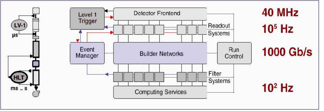
The architecture of the Trigger/DAQ system of CMS is made in a modular structure based on 8 basic slices that can be inserted to match the output of the L1 trigger system. Each slice can process up to 12.5 kHz of events read from the Level-1 trigger. The system can run with one slice only up to the full 8 slices that allow the processing of the nominal L1 throughput. This approach is particular suitable during the initial LHC luminosity since the full potentiality of the Trigger/DAQ system is not needed. As for ATLAS, this scheme allows also the deferral scenarios of the Trigger DAQ system to allocate financial resources needed for others CMS subdetectors on a critical path. More details on the CMS High-Level Trigger (rates and acceptances for various physics channels) are reported in [12].
10.50 The simulation of events from p-p collisions
A. Giammanco, A. Perrotta
Samples of simulated events are heavily used for the interpretation of the data collected by high energy experiments to determine the expected distributions of the particles in the final states accounting for experimental effects like the resolution of the detectors or the efficiency of selection cuts used to isolate a particular final state. The simulation of an “event” requires:
- -
the generation of the four-momenta of the particles in the final state;
- -
the simulation of the interaction of the generated particles with the detector;
- -
the simulation of the digitization phase, i.e. the process by which analogic electronic signals resulting from the particle-material interaction, get shaped, discriminated and read out by dedicated electronic devices
- -
running on the simulated digitized signals the programs which mimics the different levels of the trigger;
- -
running on the simulated digitized signals the programs for the reconstruction of the event both at the local subdetector level and to build the higher level analysis objects used for the final physics analysis.
If the output of the simulation after the digitization phase has the same format as the really collected raw data, the same reconstruction software as used on the real data can be applied to simulated ones. Effects as electronic noise in the detectors, event overlapping (“pile-up”), instrumental dead-times, etc., must be properly taken into account to provide realistic reconstructed analysis objects. Figure 10.127 summarizes the various steps leading to the final high level analysis objects of a typical LHC general purpose experiment, starting either from a real collider interaction or from a Monte Carlo generated event.

A particle (a muon, for example, that crosses the whole detector as shown in Figure 10.128) passes through several layers of different subdetectors, built with different materials; it passes through passive material like the cables, the magnet, the mechanical support structure; it enters also regions with different values of the magnetic field. All those effects and materials must be properly taken into account for a precise detector simulation3636 36 Quite often, the very final arrangement for auxiliary equipments, like cables, shieldings, etc., is not finalized until the detector is fully built and closed, thus leading to some new “final” simulation samples to be produced only when the correct account of the crossed material is known..

High level of details and precision can be achieved with an accurate full simulation. Detector responses can further be validated and tuned with: test beam data; in situ calibration data (e.g. cosmics, halo muons); calibration data from LHC collisions (, , , etc.). As experiments get more complex, also their simulations become more complex and CPU-time consuming. Therefore, while for several tasks the most possibly detailed simulation is advised, there are many where the required level of precision makes more suitable a less detailed but much quicker simulation, the so-called fast simulation. Domains where a fast simulation is more suitable than a full one are:
- -
quick and approximate estimates of signal and background rates;
- -
fast development of analysis methods and algorithms;
- -
test of new generators or new theoretical ideas in a realistic environment;
- -
scan of complex, multi-parameter spaces (like e.g. SUSY);
Emulation of intermediate quantities, as digitized or reconstructed detector hits, could also be provided. Figure 10.129 compares the job done by a fast simulation with what done by a full simulation.

Fast simulation emulates the combined result of detector simulation and reconstruction, and it is therefore generally tuned and validated with the full simulation results (while full simulation is tuned and validated with the real data).
10.50.1 Full simulation of the main detectors components
In the following paragraphs the way how the main components of the ATLAS and CMS detectors are accounted for in the full simulation will be outlined and then compared with the methods used in the fast simulation. Details on the two detectors and their simulation and reconstruction software can be found in [18, 19] for ATLAS and [20] for CMS.
Simulation of the inner tracker systems
A charged particle crosses the active layers of the inner tracking detectors (silicon strips and pixels in CMS; silicon strips, pixels and an outer transition radiation detector in ATLAS). Propagation is affected by multiple scattering in the detector and surrounding material. Within each detector layer, the particle looses energy along the path between its entry and exit point. The produced charges are collected causing a signal in the dedicated electronics (Figure 10.130a). Gaussian noise is added on top of those signals, and also to the other channels not interested by the trajectory of any particle (Figure 10.130b). In the same event other particles add up, coming from the very same generated event, multiple interactions, in-time or out-of-time pile-up (Figure 10.130c). All charges are linearly added up in case of overlap, then discriminated and digitized, ending up with the raw data of the tracking detector layers. Those raw data, separated from the information of the generated particles, are the input for the reconstruction phase (Figure 10.130d). Tracking algorithms apply pattern recognition and track fit; magnetic field, multiple scattering, material effects are also taken into account. Different use cases can be considered: low/high , searches for displaced vertices, etc. At the end of the reconstruction (as for the real data) the exact 1-to-1 correspondence between generated charged particles and reconstructed tracks is generally lost, and it can only be restored on a probabilistic basis.

Simulation of the calorimeters
Electrons and photons in the electromagnetic (ECAL) and hadrons in the hadronic (HCAL) calorimeters generate large showers, respectively via pair production and bremsstrahlung processes, see Figure 10.131, and via hadronic interactions.

On the other hand electromagnetic and hadronic
calorimeters are coarser grained detectors if compared to the tracking devices.
To perform a realistic simulation, several effects must be taken into
account, i.e. for electromagnetic calorimeters:
variation of the light collection along the length of the crystal
(homogeneous ECAL) or of the fibers (sampling ECAL); modified crystal
transparency with large integrated doses (homogeneous ECAL); noise;
electronic thresholds. Simulation parameters must be tuned to reproduce the results of the test beams.
The whole charge collected in one, or even more than one, crystal or tile is read out together.
Therefore, in the reconstruction, exact 1-to-1 correspondence between generated and reconstructed
particles is lost and cannot be restored3737
37
The exception being isolated electrons,
photons or hadrons at low luminosity.
Clusters of energy deposits in the HCAL represent the jets,
which are the high level analysis objects obtainable starting from the calorimetric showers;
different clusterization algorithms and recombination schemes are available, depending on the
needs of the specific analysis.
Simulation of the muon detectors
Muon detectors are tracking devices placed in the outer part of the detector and exploiting the large penetrating power of muons. Passing muons produce ionization charge in the drift cells; charges drift towards the sense wires with a drift velocity which is in general dependent on the impact position, muon direction, residual magnetic field. Contributions from electronic noise, neutron background, halo muons, muons from pile-up events (in-time or from a different beam crossing), punch-through hadrons, must be taken into account. Local reconstruction starts in a single layer and continues by correlating track segments in the different substructures. Global reconstruction matches these local segments with those of the inner tracking system (plus possibly signals from the calorimeters that must be compatible with the particle being a minimum ionizing particle). Exact 1-to-1 correspondence between generated and reconstructed muons is formally lost although, given the lower track density, there is the matching probability is higher than in the inner tracker.
Simulation of the trigger
As mentioned in Section 10.49, ATLAS and CMS achieve rate reduction by means of their L1 and HLT trigger systems: events rejected by the trigger are lost forever. The simulation must reproduce the trigger decision: it is not necessary to actually drop all events that do not pass the trigger, but it must be made clear which can be used for the analysis, and which cannot. Since the HLT reconstruction algorithms are similar but not generally the same as those used in the off-line analysis, as for example they cannot access the whole calibration data-base, to obtain realistic performance in the simulation code specialized trigger modules must be developed.
Timing
To obtain the high level of details and precision of the full simulations a considerable amount of CPU time is required. As an example, for CMS it was estimated [21] that for a typical LHC high- p-p collision in a 1 GHz Pentium III3838 38 To obtain the corresponding values in kSI2k-sec, the standard CPU speed normalization between machines based on the SPECint®2000 benchmark for integer calculations, those times obtained with a 1 GHz machine must be multiplied by a factor 0.46. the required processing times were:
- -
less than 100 ms/evt for the Monte Carlo event generation;
- -
100-200 s/evt for the simulation of the material effects;
- -
1-10 s/evt for the digitization (simulation of the read-out electronics);
- -
10-100 s/evt for the reconstruction.
Therefore, the total CPU-time spent before the analysis can start ranges from 3 to 5 minutes per event. Those estimates were done with the previous framework and event data model of CMS: it is expected, however, that timings will not change that much with the new CMS simulation code. The CPU time needed for the event simulation in the present release of the ATLAS software can be derived from Figure 10.132 [22], for different types of events and as function of the largest absolute value of the pseudorapidity simulated (in a p-p collider the track density, and therefore the CPU time needed to simulate the complete event, increases strongly with pseudorapidity).

10.50.2 Fast simulation in ATLAS
ATLFAST [23] is the package for fast simulation developed and used in ATLAS. It includes most crucial detector aspects, as jet reconstruction in the calorimeter, momentum and energy smearing for electrons and photons, effect of the magnetic field, and missing energy. It provides, starting from the generated particles, the list of reconstructed jets, isolated leptons, photons, muons, and missing transverse energy. It provides also (optionally) the list of reconstructed charged tracks. No particle propagation, nor interaction with the detector material is simulated; a coarse detector geometry is considered to define the acceptances. Fast simulation in ATLAS is therefore obtained by smearing directly the Monte Carlo truth informations with efficiencies and resolutions as obtained from the full simulation.
Tracking
Emulation of track reconstruction is provided (only optionally) for charged particles inside the inner detector. It is obtained by smearing three-momenta and impact parameters, as indicated in the full simulation studies, with different parameterizations of the smearing and of the reconstruction efficiency for muons, pions and electrons.
Calorimetric clusters
In the present implementation, all electron or photon energy is deposited in one single ECAL cell, and all hadrons energy in one single HCAL cell. A new parameterization has been studied [24] and is ready to be implemented. In this new parameterization, the transverse energy of all undecayed particles is summed up in cells having the same granularity as the calorimetric L1 trigger (), which is coarser than the granularity of the full simulation; the longitudinal segmentation is limited to the separation between ECAL and HCAL. The effect of the 2 T magnetic field is taken into account. Generic calorimetric cluster reconstruction is started from those cells, and an appropriate energy smearing and reconstruction efficiency is applied after cluster identification from Monte Carlo truth as electron, photon or hadron.
Jets
Calorimetric clusters non associated with isolated or are associated into jets and further smeared, with a parameterization which depends on the presence of quarks of a given flavour in the generated particles that originated the calorimetric clusters. Different parameterizations are also applied for different luminosity scenarios, reflecting the different amount of pile-up. Reconstruction and tagging efficiencies are not included in ATLFAST, but they can be applied “by hand” at a later stage.
Muons
Three possibilities are foreseen for the parameterization of the momentum resolution, depending on the subdetectors used for the muon reconstruction: muon system stand-alone, inner detector stand-alone, or the two combined. Muons can be flagged as isolated or non-isolated. Muon tagging efficiency is not included in ATLFAST, but it can be applied at a later stage.
Trigger
Only primitive trigger routines are considered, not meant to cover all ATLAS triggers and levels. They are aimed essentially at eliminating events which have no chance of passing ATLAS L1 and L2 triggers.
Pile-up
Pile-up events are not simulated in ATLFAST, but a different smearing of jets due to pile-up is provided as a function of the luminosity, see Figure 10.133. Also the parameterization of the trigger selection allows for the low and high luminosity options ( cm-2s-1 and cm-2s-1 respectively).

Timing
A very fast processing is obtained thanks to the approach chosen in ATLFAST of relying on parameterizations of the properties of the final analysis objects, without simulating interactions of particles with the detector material, nor attempting any reconstruction. A gain of about four orders of magnitude is claimed with respect to fully simulated similar events, which corresponds to a computation time of just a few hundred milliseconds per event.
10.50.3 Fast simulation in CMS
CMS software [20] has recently completed the migration from the previously adopted framework to the present one. We describe here the package FAMOS for the fast simulation of particle interactions in the CMS detector, based on the old framework; its main features will however remain basically unchanged in the new framework.
The output of FAMOS is designed to be as close as possible to the output of the full simulation and reconstruction of CMS. It delivers the same physics objects (calorimetric hits and clusters, tracker hits, and reconstructed tracks and muons), with identical interface: they can be used as inputs of the same higher-level analysis algorithms (-tagging, electron, muon and tau candidates, jet clustering, lepton isolation, etc.) as the real or fully simulated data.
Particles in FAMOS are propagated in the nominal magnetic field through the inner tracker and up to the entrance in the calorimeters. The following interactions are simulated in the tracker material:
- -
electron bremsstrahlung;
- -
photon conversion;
- -
energy loss by ionization for charged particles;
- -
multiple scattering for charged particles.
Electron, photon and hadron showering is allowed in the ECAL and HCAL. Nuclear interactions are not simulated in FAMOS3939 39 Their implementation is indeed foreseen in the new fast simulation., which implies that hadronic showers never initiate before the calorimeters, and there is a lower number of secondary vertices. As will be described in section 10.50.4, this implies in turn a different -tagging significance with respect to the full simulation which needs therefore a separate tuning.
Tracking
Charged particles in FAMOS are traced through a simplified detector geometry. The inner part of CMS is treated as composed by thin cylindrical layers of pure silicon, whose thickness is tuned on the number of bremsstrahlung photons with MeV radiated by energetic electrons traversing any such layer. A comparison of the material content of the inner CMS in FAMOS and in the full simulation is shown in Figure 10.134, where the photon conversion points in the plane - are recorded.


Charged particles in FAMOS propagate in the magnetic field through the tracker layers; multiple scattering and energy loss by ionization are taken into account. Intersections between simulated trajectories and tracker layers give the “simulated hits”; they are then smeared and turned, with a given probability, into “reconstructed hits”. An emulation of seeding and pattern recognition is performed with the reconstructed hits originating from a given propagated particle, followed by a fit of the track done with the same fitting algorithms used the reconstruction of full simulated events.
Calorimeter response to and
In FAMOS, the simulation of an electron shower makes use of the Grindhammer parameterization [25], implemented in the GFLASH code [26]. The photon case goes back to the electron case after the first splitting. Shower develops as if the whole ECAL were a homogeneous medium. The energy deposits are sliced longitudinally; in each slice energy spots (calorimeter hits) are distributed in space according to the radial profile and placed in the actual crystal geometry. The following effects are simulated: leakage (which is propagated to the HCAL), gaps between ECAL modules, shower enlargement due to the B-field, electronic noise and zero suppression. Starting from the calorimeter hits, clustering is obtained as in the reconstruction of full simulated events.
Calorimeter response to hadrons
Charged and neutral hadrons propagate to the ECAL and HCAL entrances. The energy response is derived from a full simulation of single pions generated at fixed values between 2 and 300 GeV. Smeared energy distributes in the calorimeter cells using parameterized longitudinal and lateral shower profiles. Other hadrons are treated as pions of the same .
Muons
Muons in FAMOS are not propagated until the CMS muon chambers. Their calorimetric response is tabulated in a similar way as for hadrons. The response of the muon chambers is parameterized on samples of fully simulated single muons (with GeV) to reproduce efficiencies and resolutions, assuming a gaussian distribution for the final quantities. Different parameterizations are provided for L1 trigger muons, HLT muons, and global muons. HLT and global muons may require a correlation with the reconstructed track.
Trigger
L1 and HLT trigger signals and primitives are obtained as a “by-product” of the fast simulation of the corresponding subdetectors. Decision functions are then reconstructed starting from those trigger primitives with the very same logic as in the real data.
Pile-up
In-time pile-up minimum bias generated events are superimposed to the signal events, and their particles treated as all other particles in the event. No out-of-time pile-up is considered.
Timing
A complete event takes a couple of seconds to be simulated and reconstructed with FAMOS (about 1 s in FAMOS itself, the rest in the analysis and framework overhead); it is slightly more with the pile-up superimposed. It consists of more than two orders of magnitude gain with respect to the full simulation and reconstruction.
10.50.4 A case study: full vs. fast simulation in CMS
A few comparisons between the former fast and full simulations of CMS (respectively FAMOS and OSCAR, based on GEANT4[26]) are shown here. Although the agreement between the results of the two simulations is good for most of the relevant observables, emphasis will be given to the remaining discrepancies, with a discussion of the possible causes.
Electrons and photons
In the fast simulation ECAL is represented as a homogeneous medium. This allows by itself such a saving of CPU time, that a relatively high degree of realism can be afforded on other aspects:
- -
a lot of details are allowed (after optimization, about 1500 hits are calculated per shower of 35 GeV);
- -
the front and rear leakage, the fraction of signal lost in the inter-module voids, and the shower spread due to the magnetic field are simulated;
- -
the calorimetric noise is added to the signals;
- -
for very high energy electrons, the punch-through into HCAL is also parameterized;
- -
fake electrons can show up when an ECAL cluster is associated with a simulated seed originating from hits produced by the tracks of the event.
The effect of all these details can be seen in Figure. 10.135: in general, the reconstructed energies in FAMOS reproduce the corresponding ones from the full simulation with an accuracy at the per mill level in the calorimeter barrel, and at the per cent level in the endcaps.
Muons
As seen in 10.50.3, the simulation of muons in FAMOS is not very refined. In spite of that, the higher-level variables show a remarkable agreement with the full simulation, one example being the invariant mass of a di-muon resonance, shown in Figure 10.136.

Fake tracks
As explained above, the tracks in FAMOS are not currently obtained from a pattern recognition procedure, but from a fit of the hits associated to a “true” charged particle. Because of this use of the Monte Carlo truth during the reconstruction step, no fake tracks (i.e., random combination of hits from more than one track, with or without the contribution of fake hits coming from detector noise) can contaminate the final sample of reconstructed tracks.
Studies in full simulation show that 0.5% of the tracks in the “low luminosity” scenario ( cm-2s-1) are fakes. At that level, the incidence of fake tracks is irrelevant for most of the LHC studies, and a realistic simulation of this combinatorial background starting from the hits would require a pattern recognition, which would result in a significant increase of CPU time.
Impact parameter and -tagging
FAMOS applies to the tracks the same -tagging algorithms applied on data and full simulation. Since the impact parameter is the key ingredient of some of the best performing -tagging algorithms, the validation of this variable (shown in Figure 10.137 for single muons) is of paramount importance. It has to be remarked that the impact parameter was not directly tuned to reproduce the full simulation shape, thus making this full/fast simulation agreement a particularly significant test.


Unfortunately, the agreement observed in Figure 10.137 is not enough to guarantee the same -tagging performance on the fast simulated events, as evidenced by the first three plots in Figures 10.138, which show the output of one high-level -tagging algorithm mainly based on the impact parameters of the charged tracks, for , and -initiated jets: the output of this algorithm in the fast simulation reproduces quite well the behavior of the full simulation for and -jets, while the same is not true for jets originating from lighter partons. This will affect all analyses in which significant sources of background come from processes where some light jets are mistagged as coming from heavy quarks. A common way to describe the performance of a -tagging algorithm is by showing its misidentification probability as function of the efficiency. Such a representation is shown in the last plot in Figure 10.138, for the fast and the full simulations of CMS: one can see that over a wide range of cuts, chosen such to fix the rejection factor for the light-flavours related background, the -tag efficiency in the fast simulation is systematically overestimated by some 5-10%.

In order to understand which, of the many simplifications meant to make FAMOS fast, is the culprit of this situation, a closer look to the variables that enter in the definition of the -tagging is needed. In Figure 10.137 we had shown how well the impact parameter was reproduced in FAMOS, in the relatively easy case of isolated muons. Figure 10.139 shows instead the largest impact parameter among all the charged tracks (mostly hadrons) in each jet. The comparison with the corresponding full simulation is not satisfactory for jets from partons. The situation improves if one does not consider the tracks with the largest impact parameter: for instance, in Figure 10.140 the third largest impact parameter in each jet is shown.


All this suggests that FAMOS lacks the description of some process which seldom produces a small number of tracks with significant impact parameter. At first, it was thought that the lack of fake tracks (see previous subsection) could have been the responsible of the discrepancy, but at a closer look they were found not sufficient to explain it. Instead, the difference can be attributed to the nuclear interactions of the hadrons with the tracker active and passive materials: they were not simulated in FAMOS, but their implementation is planned for the next release of the fast simulation of CMS.
Hadrons and jets energy
The calorimetric response (ECAL+HCAL) to single pions in FAMOS and in the CMS full simulation is shown in Figures 10.141a and b. In order to simplify the simulation, all the long-lived hadrons in FAMOS are treated as charged pions. This proves to be enough to obtain a remarkable agreement with the full simulation, as shown in Figure 10.141c for jets between 80 and 120 GeV/ in . There are plans, however, to further improve the realism, by treating differently: the long-lived neutral hadrons, since they don’t release any signal before the first nuclear interaction; protons and neutrons, whose kinematic is different due to the high mass; anti-protons and anti-neutrons, which in addition can annihilate.


Bibliography
- [1]
ATLAS Muon Spectrometer Technical Design Report; CERN/LHCC/97-22, 5 June 1997;
ATLAS Detector and Physics Performance Technical Design Report; CERN/LHCC/99-14/15;
The ATLAS Experiment at the CERN Large Hadron Collider, submitted to JINST on December 24, 2007. - [2] CMS Physics Technical Design Report, Volume 1; CERN/LHCC/2006-001, CMS TDR 8.1, 2 February 2006.
- [3] M. Aharrouche et al., Energy linearity and resolution of the ATLAS electromagnetic barrel calorimeter in an electron test-beam, Nuclear Instruments and Methods in Physics Research A 568 (2006) 601-623.
- [4] G. C. Blazey et al., hep-ex/0005012v2 (2000)
- [5] S. Catani et al., Phys. Lett. B285 291 (1992)
- [6] A. Heister et al., CMS NOTE 2006/036 (2006)
- [7] R.Wigmans, “Calorimetry”, published by Clarendon Press, Oxford Science Publications (2000)
- [8] V.Konoplianikov et al., CMS NOTE 2006/042 (2006)
- [9] ATLAS Collaboration, “ATLAS High-Level Trigger, Data Acquisition and Control Technical Design Report”, CERN/LHCC/2003-022, June 2003.
- [10] F. Parodi, private communication.
- [11] CMS Collaboration, “CMS The Tridas Project Technical Design Report”, CERN/LHCC/2000-038, December 2000.
- [12] N. Amapane, private comunication.
- [13] CMS Physics TDR, Volume 1,CERN-LHCC-2006-001
- [14] M. Heldmann, D. Cavalli, “An improved identification for the ATLAS experiment”, ATL-PHYS-PUB-2006-008
- [15] G. Bagliesi et al., “Tau jet reconstruction and tagging at High Level Trigger and off-line”, CMS-NOTE 2006-028
- [16] E. Richter-Was, T. Szymocha, “Hadronic identification with track based approach”,ATL-PHYS-PUB-2005-005
- [17] CMS Collaboration, CMS High Level Trigger, CERN/LHCC 2007-021, LHCC-G-134
- [18] ATLAS Collaboration, “ATLAS Detector and Physics Performance, Technical Design Report, vol. 1”, ATLAS-TDR-014, CERN-LHCC-1999-014.
- [19] ATLAS Collaboration, “ATLAS Computing Technical Design Report”, ATLAS-TDR-017, CERN-LHCC-2005-022.
- [20] CMS Collaboration, “CMS Physics TDR, vol. 1: Detector Performance and Software”, CMS-TDR-8.1, CERN-LHCC-2006-001.
- [21] S. Wynhoff, “FAMOS, a dynamically configurable system for fast simulation and reconstruction for CMS”, talk from CHEP03, La Jolla, Ca, USA, 2003, arXiv:physics/0306052.
- [22] A. Rimoldi, private communication.
- [23] E. Richter-Was, D. Froideveaux, L. Poggioli, “ATLFAST 2.0, a fast simulation package for ATLAS”, ATL-PHYS-98-131.
- [24] K. Mahboubi, K. Jacobs, “A fast parameterization of electromagnetic and hadronic calorimeter showers”, ATL-SOFT-PUB-2006-001.
- [25]
G. Grindhammer, M. Rudowicz and S. Peters,
“The fast simulation of electromagnetic and hadronic showers”,
Nucl. Instr. and Meth. A 290 (1990), 469;
G. Grindhammer, S. Peters, “The parameterized simulation of electromagnetic showers in homogeneous and sampling calorimeters”, presented at International Conference on Monte Carlo Simulation in High-Energy and Nuclear Physics, Tallahassee, Fl, USA, 1993, hep-ex/0001020. - [26]
S. Agostinelli et al., “GEANT4, a simulation toolkit”,
Nucl. Instr. and Meth. A 506 (2003), 250;
J. Allison et al., “GEANT4 Developments and Applications”, IEEE Trans. on Nucl. Sci. Vol. 53. N. 1 (2006), 270.