Counting elements and geodesics
in Thompson’s group
Abstract
We present two quite different algorithms to compute the number of elements in the sphere of radius of Thompson’s group with standard generating set. The first of these requires exponential time and polynomial space, but additionally computes the number of geodesics and is generalisable to many other groups.
The second algorithm requires polynomial time and space and allows us to compute the size of the spheres of radius with . Using the resulting series data we find that the growth rate of the group is bounded above by . This is very close to Guba’s lower bound of [16]. Indeed, numerical analysis of the series data strongly suggests that the growth rate of the group is exactly .
Keywords:
Group growth function , growth series , geodesic growth series , Thompson’s group2008 MSC
20F65 , 05A051 Introduction
Let be a group with finite generating set . Recall that is the (spherical) growth function for if is the number of elements in the sphere of radius of the corresponding Cayley graph. Define the (spherical) geodesic growth function to be where is the number of all geodesics of length in the Cayley graph [14]. In this article we give two quite different algorithms to compute the growth function of Thompson’s group . The first, Algorithm A, applies to a range of groups, and computes both and . It runs in exponential time and polynomial space, and is implemented to compute the first 23 terms of both functions with moderate computer resources. This algorithm is based on a random sampling algorithm developed by the third author and van Rensburg for problems in lattice statistical mechanics [21].
The second algorithm, Algorithm B, is specific to Thompson’s group , and computes in polynomial time and space. It is based on the forest diagram representation of elements of , introduced by Belk & Brown [1], and the associated length formula, which itself is based on work of Fordham [13]. We implemented this algorithm and were able to compute the first 1500 terms of , again with moderate computer resources. This data enables us to obtain an upper bound of on the growth rate of , which differs by only from the lower bound of obtained by Guba [16]. Based on this and other numeric evidence, we conjecture that Guba’s bound is indeed the correct growth rate. Both sets of data (the growth up to 1500 and geodesic growth up to 22) are published on the Online Encyclopedia of Integer Sequences as A156945 and A156946 [23].
Note that when the spherical (geodesic) growth is exponential, the growth rate coincides with the usual growth and geodesic growth rates which count the number of elements (geodesics) of length at most rather than exactly .
Many researchers have made an attempt to compute the growth of Thompson’s group. Guba [16] used a brute force technique to compute the first 9 terms of the growth series. This was extended to the first 13 by Burillo, Cleary and Weist [5]. Matucci considered a system of recurrences obtained by considering forest diagrams in his thesis [20], which turned out to be quite complicated. It is possible that his approach could be used to compute the growth series but this does not appear to have been pursued. Our own approach is to set up an algorithm (being Algorithm B) that enumerates the number of elements in the sphere of radius by computing the number of forest diagrams of weight . Using this we have been able to compute a large number of terms. One key ingredient in our algorithm is the encoding of forest diagrams by labelling both the gaps between leaves (as Belk & Brown do) as well as the internal nodes of trees, which is based on an encoding of binary trees described in [12].
Unfortunately, we have not been able to leverage our algorithm into a closed form expression for the growth function or the corresponding generating function. However, an analysis of our data indicates that the series does not correspond to a simple11 1 ie satisfying an equation of low order which has coefficients of low degree. rational, algebraic or differentiably-finite generating function (satisfying a linear ordinary differential equation with polynomial coefficients — see [24]). It is entirely possible that the generating function lies outside these classes of functions and that no reasonable closed form solution exists. See [3, 4] for examples of problems with similar (but far simpler) recurrences that have surprisingly complicated solutions.
The paper is organised as follows. In Section 2 we describe the first algorithm, which computes in exponential time the coefficients of the growth and geodesic growth functions of any group with an efficient solution to a certain geodesic problem. We apply this to Thompson’s group and display our results. In Section 3 we describe the second, polynomial time algorithm which we have used to compute the first 1500 terms of the growth function of . We describe the forest diagram construction, how it leads to our enumeration algorithm, and give the results. We then prove an upper bound for the growth rate. In Section 4 we summarise our findings, and in Appendix A we give more detailed pseudocode for our algorithms.
We work with the presentation
for Thompson’s group . We refer the reader to [6] and [7] for an introduction to Thompson’s group.
The authors thank José Burillo, Sean Cleary, Martin Kassabov, Manuel Kauers, Francesco Mattucci, Buks van Rensburg and Jennifer Taback for fruitful discussions and ideas, and the anonymous reviewer for their careful reading and very helpful feedback.
2 Algorithm A
We begin with the following lemma, due to the third author and van Rensburg in [21], which arises in the context of randomly sampling self-avoiding walks and polygons using a generalisation of the Rosenbluth method [18, 22]. In particular, it allows us to enumerate objects without having to use a unique construction.
Definition 1.
Let be a group with finite generating set . Given a word in the generators of the group define
where is the geodesic length of the element represented by . These are the subsets of the generators that shorten, lengthen and do no change the geodesic length. Note that if the group only has relations of even length (as is the case for ) then .
Lemma 2 (From [21]).
Let be the set of all geodesic words of length . Given a word from this set, let be its prefix of length . The size of the sphere of radius (ie the number of distinct elements whose geodesic length is ) is given by
Proof.
We prove this result by induction on . When , the set of geodesics is just the set of generators and so expression is true.
Let be an element of and let be the set of geodesic paths from the identity to . It then suffices to show that
Every geodesic ending at can be written as the product of a geodesic in and a generator. Thus we can write
The inner sum is zero when the set is empty. The induction hypothesis implies that the inner sum is equal to when the set is non-empty (ie when ). Exactly of the sets are non-empty and so the result follows. ∎
2.1 Description of the algorithm
The above lemma allows us to compute the size of much more efficiently than brute-force methods. The time complexity is proportional to the size of and the time to compute . The memory required is significantly reduced; we only require space to compute and the current geodesic word. This is substantially better than brute force methods; we do not have to store normal forms for all the elements in .
Suppose that has an inverse closed generating set of size , and that there is an algorithm to compute for any geodesic in this generating set. Fix an order on the generators of (this also fixes a lexicographic order on the set of all geodesic words). Then the following algorithm computes the number of elements of length .
Algorithm A. Outputs the number of elements in the th sphere.
Set a counter to 0.
Starting from the empty word, run through all geodesics of length .
Given the current geodesic, , compute for each length prefix of , and add to the counter.
By Lemma 2 the final value of the counter is the number of elements in the sphere of radius .
There are a number of ways of running through the list of all geodesics; perhaps the simplest is to traverse all the geodesics in lexicographic order using a recursive depth-first algorithm (see the pseudocode for ComputeGeod() and ComputeSphere() in Appendix A.1). It can also be done using a slightly more involved iterative procedure that given a geodesic finds the next geodesic in the lexicographic ordering (see the pseudocode for NextGeod() also in Appendix A.1).
Note that the above algorithm is easily modified to obtain the number of geodesics of length : rather than adding to the counter each time, simply add .
Proposition 3.
The time complexity of Algorithm A is , multiplied by the time to compute at each step. The space complexity is linear plus the space required to compute .
Proof.
As we run through all geodesics , we only need space to store the current geodesic word, which requires linear space, plus the space required to compute . Since we must consider all geodesics, the time is proportional to the number of geodesics in , multiplied by the time to compute at each step. ∎
So the time and space complexity of the algorithm depends on the complexity of computing and . This naturally leads to the geodesic problems described in the next section.
2.2 Geodesic problems
Algorithm A gives a memory-efficient procedure to compute growth and geodesic growth for any group that has an efficient solution to the following problem:
Problem 1.
Given a geodesic and generator , determine if or .
Note that if all the relators in have even length then these are the only two possibilities, since if means there must be an odd length relator. So the problem turns into the decision problem:
Problem 2.
Given a geodesic and generator , decide if .
If has a polynomial time and space algorithm to answer Geodesic Problem 1, then Algorithm A computes both and in exponential time, but polynomial space (assuming grows exponentially). In [9] the authors consider these problems in more detail, and prove that they imply a solvable word problem for groups whose set of relators is countably enumerable. Note that if a group has an efficient solution to its word problem, then a naive brute force computation of and would still require an exponential amount of memory (assuming the functions and are exponential), so a polynomial space algorithm is a marked improvement on this.
2.3 Thompson’s group
For Thompson’s group , one can use the geodesic length formula of Fordham [13] to compute the length of any word in polynomial time and space. There are now other similar formulations, and we note those due to Guba [16] and Belk & Brown [1]. We chose to base both of our algorithms on the forest diagrams of Belk & Brown as we found them the easiest to implement. We note that there is a simple bijection between this representation and binary tree pairs. It is possible to develop similar algorithms based on the Fordham and Guba formulations, but we have not pursued these possibilities because we believe that they will give very similar results.
We start our description of the algorithm by first explaining the forest-diagram length formula of Belk & Brown (we refer the reader to the original paper [1] for a fuller explanation). In Figure 1 we describe some of the terminology associated with this formula.

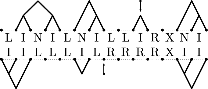
It consists of two rows of forests of binary trees, above and below two rows of labelled gaps. One (possibly empty) tree in each forest is pointed and the diagram cannot contain “common carets” (see Figure 1). A pair of carets in a given column are considered to be common carets, if they are both immediate neighbours of the gaps. Further, the extreme left and right columns of the diagram cannot be empty. Each element of corresponds uniquely to such a forest diagram with no common carets.
The labels of the gaps are determined by the structure of the forests. We found it convenient to make a slight modification of the original labelling rules; we label gaps by applying the following rules in order:
- (i).
“L” if it is left of the pointer and exterior (outside a tree),
- (ii).
“N” if it is immediately left of a caret and interior (inside a tree),
- (iii).
“X” if it is immediately left of a caret and exterior,
- (iv).
“R” if it is right of the pointer and exterior,
- (v).
“I” if it is interior.
Belk & Brown give “N” and “X” the same label, however the above labelling means that “L”, “R” and “X” are always exterior, while “I” and “N” are always interior. The length of a group element represented by a diagram is then
| (1) |
where is the weight of a column as given in Table 1. We refer to this sum as the weight of a given forest diagram.
| I | N | L | R | X | |
|---|---|---|---|---|---|
| I | 2 | 4 | 2 | 1 | 3 |
| N | 4 | 4 | 2 | 3 | 3 |
| L | 2 | 2 | 2 | 1 | 1 |
| R | 1 | 3 | 1 | 2 | 2 |
| X | 3 | 3 | 1 | 2 | 2 |
Our table differs from that in Belk & Brown [1] also in that our table entries include the contribution from the number of carets, whereas Belk & Brown add this contribution separately.
It should be noted that labels are defined very locally; to label a given column we do not need to know the labels of columns far away. While this is not crucial for Algorithm A, it is critically important for Algorithm B as it allows us to build a diagram with its labels column-by-column. This will be discussed further below.
2.4 Implementing Algorithm A for Thompson’s group
Propositions 3.3.1 and 3.3.5 of [1] describe how multiplication by each of the generators and their inverses changes a forest diagram. Multiplying a reduced forest by simply moves the top pointer one tree to the right or left which can be done in constant time. Multiplying by adds a single caret to the roots of two adjacent trees, then canceling common carets if they exist. Multiplying by either adds or deletes a caret in the bottom or top forests, and then cancels common carets if they exist. Note that after multiplying by at most a single common caret exists.
So a word of length produces a forest of at most carets, so we can store the forest diagram for such a word in space . We can turn this into an algorithm to compute the geodesic length of an element of as follows:
Algorithm GeodesicLengthF. Computes the geodesic length of an element in
Input a word of length in the generators .
Start with the empty forest diagram (no carets, and both pointers at the 0 position).
For each letter of , redraw the current forest diagram by multiplying by this letter. To do this one must scan through the stored diagram and possibly add or delete a caret; this takes operations.
When all letters are read, compute the weight of the resulting diagram by labelling it (which takes operations) then read the geodesic length off from the table (which takes operations).
Proposition 4.
One can compute the geodesic length of a word in in time and space .
Proof.
We store the forest diagram as a pair of two trees, and use depth-first search to run through the trees. The size of the tree is and it takes steps to scan through and reduce a pair of common carets. So as we run through each letter of we perform steps, so all together . The final step takes to label the forest diagram and to compute the weight. ∎
The above algorithm allows us to quickly compute the geodesic length of any element of (and so ); it formed the basis of our implementation of Algorithm A. This then allowed us to calculate both the growth function and geodesic growth function for Thompson’s group up to length . See Table 3. Since has exponentially many geodesics (it has exponential growth) the time for Algorithm A is exponential, but space is .
| 0 | 1 | 1 | 12 | 431238 | 556932 |
| 1 | 4 | 4 | 13 | 1180968 | 1588836 |
| 2 | 12 | 12 | 14 | 3225940 | 4507524 |
| 3 | 36 | 36 | 15 | 8773036 | 12782560 |
| 4 | 108 | 108 | 16 | 23809148 | 36088224 |
| 5 | 314 | 324 | 17 | 64388402 | 101845032 |
| 6 | 906 | 952 | 18 | 173829458 | 286372148 |
| 7 | 2576 | 2800 | 19 | 467950860 | 804930196 |
| 8 | 7280 | 8132 | 20 | 1257901236 | 2255624360 |
| 9 | 20352 | 23608 | 21 | 3373450744 | 6318588308 |
| 10 | 56664 | 67884 | 22 | 9035758992 | 17654567968 |
| 11 | 156570 | 195132 |
In [16] Guba proves that the growth rate of the number of elements in Thompson’s group is bounded below by , which also serves as a lower bound for the growth rate of geodesics. We can use our data to obtain upper bounds for both growth and geodesic growth.
Since every element of length is the concatenation of some element of length and some element of length , it follows that and so the sequence is submultiplicative. The same is true for the sequence , which counts the number of geodesics. Fekete’s lemma [26] states that if a sequence is submultiplicative, then the sequence is monotonically decreasing, which means that for any fixed , the number is an upper bound on the limit of . From this we obtain the following:
Proposition 5.
The growth rate for the growth function of Thompson’s group satisfies the bounds
| (2) |
Similarly, the growth rate for the geodesic growth function of Thompson’s group satisfies the bounds
| (3) |
In the next section we will sharpen the upper bound for the growth of elements considerably.
3 Algorithm B
In this section we describe a second algorithm to compute the number of elements in the sphere of radius in Thompson’s group with standard generating set; this algorithm runs in polynomial time and space.
Recall the forest diagram definition from the previous section. We count forest diagrams by their length using a column-by-column construction. Such constructions have been used to great effect in combinatorics and statistical mechanics yielding closed form solutions (for example [25, 2]), polynomial time algorithms (for example [8]) and exponential time algorithms that are exponentially faster than brute force methods (for example [11]). The construction we use here gives rise to a system of recurrences which is rather cumbersome. As such, we do not give these recurrences explicitly, but instead iterate them using Algorithm B.
An incomplete forest diagram can be thought of as a forest diagram with all rightmost columns deleted after some point. In order to append a column in a “legal” way we only need to keep track of the labels of the rightmost column and two numbers which measure how far the top and bottom trees are from being “complete”.
3.1 Encoding and counting binary trees
Since the forest diagrams consist of a pair of sequences of binary trees, the starting point for our enumeration algorithm is to find an efficient encoding of binary trees. Binary trees are counted by the Catalan numbers and there is a large number of encodings. We have chosen one that naturally reflects the column-by-column construction used.
We start by labelling leaves and internal nodes of the trees by “N”, “I”, “n” and “i” as shown in Figure 3. By convention we will not label the left-most leaf.

Reading these labels from left to right gives a word in the alphabet which starts with an “n” and alternates lower and upper case letters. The tree in Figure 4 is encoded by the word “nInNiInNnIiI”.

This labelling was used in [12] and they proved that each tree has a unique encoding. The following lemma is Theorem 4.4 in that paper with modified notation.
Lemma 6.
A word, , encodes a non-empty tree if and only if
- (i).
it starts with “n”,
- (ii).
ends with “I”,
- (iii).
alternates lowercase and uppercase letters,
- (iv).
all of its prefixes satisfy (where denotes the number of occurrences of “y” in )
- (v).
.
Proof.
For the purposes of the proof we prepend an initial “N” to all encoding words. Call a word on admissible if it has an initial “N” and it satisfies the 5 conditions above when the initial “N” is deleted.
Consider the mapping that associates a binary tree of carets to the word of length obtained by starting with an “N” and then reading the labels from left to right (see Figure 4). We show by induction on that is bijective onto admissible words of length .
For , this is evident, there is a unique tree with one caret, which is mapped by to the unique admissible word of length , namely “NnI”.
Assume that the bijection holds for and we will show that it also holds for . First we check that the image of a tree with carets is admissible. Let be a tree obtained from by deleting two leaves adjacent to the same caret (so becomes a leaf in ) and let . As seen in Figure 5, is equal to where an upper-case letter “A” is replaced by the 3-letter factor “NaI”, where “a” is the lower case of “A”. Since is admissible (by induction), it follows that is also admissible.

Now to prove that is bijective consider an admissible word of length and we will show that it has a unique pre-image. Let be the word obtained from by keeping only its upper-case letters. Since starts with “N” and ends with “I” it must contain a factor “NI". This lifts to a 3-factor “NaI” in the word . Replacing this 3-factor by a single letter “A”, where “A” is the upper-case of “a”, we obtain a word of length . It follows that is also admissable.
Moreover one may verify (see Figure 5) that any pre-image of must be obtained from a pre-image of where the leaf corresponding to “A” is replaced by a caret with two leaves below it. Since there is a unique pre-image of (by induction), there is also a unique pre-image of . ∎
We can now count binary trees by counting admissable words in this alphabet. Define the size of an even-length word to be its half-length. Following from condition (iv) above we define the excess of a word, , to be the quantity . So appending “nN” increases the excess by , appending “nI” or “iN” does not change the excess and appending “iI” decreases the excess by . Further, appending any of these pairs increases the size by ..
Corollary 7.
A word encodes a nonempty binary tree if and only if its excess is zero.
Proof.
This follows from condition (v) above. ∎
Given an even length word and its excess we can decide which pairs can be legally added to the word — in fact there is little restriction other than when the excess is , in which case one may not append iN or iI since this violates condition (iv). Thus one can construct a recurrence satisfied by , the number of valid words of length (size ) and excess .
- (i).
There is a single valid code word of size , namely “nI”. Hence .
- (ii).
Any word with excess equal zero can be extended by
- (a)
appending “nN” which makes its excess 1, or
- (b)
appending “nI” which leaves its excess 0.
- (a)
- (iii).
Any word with excess strictly greater than zero can be extended by
- (a)
appending “nN” which increases its excess by 1, or
- (b)
appending “nI” which leaves its excess unchanged, or
- (c)
appending “iN” which leaves its excess unchanged, or
- (d)
appending “iI” which decreases its excess by 1.
- (a)
This translates into the following recurrence.
| (4) | ||||
| (5) |
While this recurrence can be solved explicitly, we show how it may solved iteratively in order to help explain our main result. Notice that the algorithm that we use to iterate this recurrence does not “look backward” and compute in terms of and , rather it “looks forward” and determines which coefficients gain contributions from . Of course this algorithm (and our main result) could be rewritten to be “backward looking” but the authors feel that this way follows more naturally from the construction.
Algorithm CountBinaryTrees. Outputs the number of binary trees of a desired size.
Input maximum size (half-length) and set size .
Set — has to store the number of words of size and excess .
At the current size run through all possible values of the excess .
If the current value of is zero then (because we can append “nN” and “nI”)
- (i).
increment by , and
- (ii).
increment by .
Otherwise (we can append “nN”, “nI”, “iN” and “iI”)
- (i).
increment by , and
- (ii).
increment by , and
- (iii).
increment by .
After running through all possible values of the excess, increment the size by and output — the number of valid complete words of the current size.
Keep iterating until the desired size is reached.
Notice that we must iterate through all values of the size and excess in order to compute the final enumeration. Since the excess is at most the size for each (possibly incomplete) forest diagram, this means that the algorithm requires time. Once we reach a given size we can forget all the data from shorter lengths. In fact we only need to remember the current size and the next size. This means the algorithm requires space.
For the main algorithm below, the labels “I” and “N” correspond precisely to the labels used in the Belk & Brown geodesic length formula. The lower case labels can then be ignored and we instead keep track of the excess and note that when appending an “N” the excess either stays constant or increases by , and when appending an “I” the excess either stays constant or decreases by . Note also that the size (which was the half-length when lower-case letters are considered) coincides with the length when the lower-case letters are ignored, so we will use the terminology of length (instead of size) from now on.
3.2 Transitions in the upper forest
We now describe how to construct the upper half of the forest diagram column-by-column; the lower half is encoded by an identical procedure. We commence every forest with an empty column labelled “L”. The possible transitions from a column with a given label to the next depend only on that label, the excess and whether one is to the left or right of the pointer. Note that the excess can only be non-zero if the label is either “I” or “N”. We now describe this transitions in detail.
We will write the last column of the current upper forest as a triple of the label, a flag indicating whether it is left or right of the pointer, and the excess. For example, a diagram ending in an “L” must be left of the pointer, and have excess 0 and so we denote it by . Call this triple the state of the upper diagram.

- (i).
If the upper forest ends in an “L” then it must be in state . See Figure 6. We may append
- (a)
“L”, which keeps the diagram in state ,
- (b)
“R”, which means the pointer is now to the left of the current position, so the diagram is now in state ,
- (c)
“X”, so again the pointer has been passed, and the diagram is in state ,
- (d)
“I”, which starts a tree with codeword “nI” so the state becomes ,
- (e)
“I” and put the pointer on the tree (just started by this “I”) and so move to the state ,
- (f)
“N”, which starts a tree with codeword “nN” so the state becomes ,
- (g)
“N” and put the pointer on the tree (just started by this “N”) and so move to the state .

Figure 7: If a diagram ends in “R” then we can either append another “R” or an “X”. On the other hand, if the diagram ends in “X” then we must start a tree with either “I” or “N”. - (a)
- (ii).
If the upper forest ends in an “R” then it must be in state . See Figure 7. We may append
- (a)
“R” which keeps the diagram in state ,
- (b)
“X” which adds a gap immediately to the left of a new tree, and moves to .
- (a)
- (iii).
If the upper forest ends in an “X” then it is in state and we must start a new tree. See Figure 7. We may append
- (a)
“N” and move to the state ,
- (b)
“I” and move to the state .

Figure 8: If a diagram ends in “I” of excess 0 then we can continue the tree with an “I” or an “N” as described in Section 3.1 (note that an internal node labelled by “n” will be created). If we are to the left of the pointer then we can append an empty column labelled “L”. If we are to the right of the pointer then we may append an empty column labelled “R” or “X”. - (a)
- (iv).
See Figure 8. If the diagram is in state then we may
- (a)
continue the current tree by appending “N” or “I” and so move to or ,
- (b)
finish the tree by appending “L” arriving in state .
- (a)
- (v).
Similarly, if the diagram is in state then we may
- (a)
continue the current tree by appending “N” or “I” and so move to or ,
- (b)
finish the tree by appending “R” or “X” and so arrive in state or .
- (a)
- (vi).
Finally, if the diagram is in state with and or then we are in the middle of constructing a tree (as described in Section 3.1). Note that one cannot have label “N” with excess zero, nor may we change . We may now
- (a)
add “N” and increase the excess by 1, moving to ,
- (b)
add “N” leaving the excess unchanged giving ,
- (c)
add “I” leaving the excess unchanged giving
- (d)
add “I”, decreasing the excess by 1, moving to
- (a)
Again, these constructions are easily turned into an algorithm and we refer the reader to the pseudocode for UpdateLeft(state) and UpdateRight(state) in Appendix A.2.
One might also attempt to write out a set of recurrences, but they are quite cumbersome; we now require several sets of coefficients since one must keep track of the excess, the final label and whether one is to the left or right of the pointer. This becomes extremely unwieldy for the full algorithm when one keeps track of the states of the upper and lower forests. Because of this we were unable to write out the full recurrences; instead we keep the recurrences implicit and iterate them using our algorithms.
3.3 The full algorithm
The full algorithm is very similar to Algorithm CountBinaryTrees, except that now the states of the upper and lower forests must be remembered and all possible pairs of transitions must be determined. The set of pairs of transitions is very nearly the Cartesian product of the set of transitions for the upper forest and the set of transitions for the lower forest; the only restriction is that we must prevent the creation of common carets.
A caret is created in the upper (lower) forest immediately above (below) a gap when a transition is made from a gap labelled “I”, “N”, or “X” to a gap labelled “I” (note that it is not possible to have a transition from “R” to “I”). Thus a pair of common carets is created when a transition is made from a pair of gaps labelled from a pair of gaps labelled by , , , , , , , or .
We iterate through the recurrence starting from a diagram that consists of a single empty column with gaps labelled by . At each iteration we examine all the possible states and consider all possible transitions from those states (avoiding common-carets) to new states using the rules described above. The contribution of diagrams of the current length is then added to the appropriate total for diagrams with new states with weight updated according to the new labels and Table 1. A forest diagram is complete when it finishes with an empty column labeled by . This should be seen to be very similar to Algorithm CountBinaryTrees except that the transitions are more complicated.
This enumerates all forest diagrams starting with an empty column labelled by and ending with another empty column labelled by . This, unfortunately, is not the precise set of diagrams that Belk & Brown considered. They considered diagrams without any empty columns at either end; Proposition 8 shows how to correct the output of the algorithm.
Algorithm B. Counts forest diagrams starting with and ending with .
Input maximum length and set length .
Set — this counter stores the number of diagrams of a given weight ending in a column with given labels and excess.
At the current length run through all the states of the upper and lower forests, , for which .
Let . This is the number of diagrams of length that end in a column in state .
Given the current state of the upper forest compute the new states that may be reached according to the rules in Section 3.2. Do similarly for the lower forest.
For each pair of transitions that does not create a common caret, compute the new length using Table 1, and increment by .
When all the states of the current length have been examined, output the number of complete diagrams, namely .
Keep iterating until the desired length is reached.
We give a more detailed account of this algorithm in pseudocode for CountForestDiagrams() in Appendix A.2. This main routine relies on the routines UpdateLeft() and UpdateRight() to compute the possible transitions. The cost analysis of the algorithm is given below in Proposition 9.
As noted above the forest diagrams enumerated by this algorithm begin with any positive number of empty columns labelled “” and then end in any positive number of empty columns labelled “”, whereas those of Belk & Brown have no such empty columns. Thankfully we can easily obtain the correct count as follows.
Let
be the formal power series with coefficients the number of forests of weight with no leading “” or tailing “” columns. Let
be the formal power series with coefficients the number of forests of weight which have a positive number (at least 1) leading “” and a positive number of tailing “” columns (which are counted by our algorithm). Note that since such forests must have weight at least 4. Then
Proposition 8.
Proof.
Let be the formal power series with coefficients the number of forests of weight with no tailing “” columns, but one or more leading “” columns. Note that since such forests have weight at least 2. Then since an empty column labelled “” increases the length of a forest diagram by . That is, we have with just one leading “” , with two leading “” , and so on.
Thus
A similar argument shows that
from which the result easily follows. ∎
3.4 Cost analysis
Proposition 9.
Algorithm B computes the number of elements in the spheres of radius up to in time and space .
Proof.
The final generating function transformation takes constant time and space, so our main concern is the complexity of enumerating a diagram with at most columns. Since each column has weight at least one, each element of the ball of radius will be represented by such a diagram.
When a new column is appended to a diagram the weight changes by at least 1 and at most 4. Thus incomplete diagrams of weight will only contribute to incomplete diagrams of weights between and . Once we have scanned through all diagrams of weight and computed all possible transitions we will not need them again and they can be thrown away. In this way we only need to store information about diagrams of five different weights at any given time. Thus the algorithm needs to store coefficients. During the iteration of the algorithm we scan through each of the diagrams of weight and compute the possible transitions; this takes operations. Since a diagram of weight may contain at most columns the algorithm requires operations.∎
3.5 Growth rate
| 0 | 1 | ||
| 1 | 4 | 4 | 4 |
| 2 | 12 | 3.464… | 3 |
| 3 | 36 | 3.301… | 3 |
| 4 | 108 | 3.223… | 3 |
| 5 | 314 | 3.157… | 2.907… |
| 6 | 906 | 3.110… | 2.885… |
| 7 | 2576 | 3.070… | 2.843… |
| 8 | 7280 | 3.039… | 2.826… |
| 9 | 20352 | 3.011… | 2.795… |
| 10 | 56664 | 2.987… | 2.784… |
| 20 | 1257901236 | 2.850… | 2.688… |
| 50 | 6015840076078706884412 | 2.726… | 2.627… |
| 100 | 2.673… | 2.6184… | |
| 200 | 2.645… | 2.618034… | |
| 500 | 2.628… | 2.6180339887498949… | |
| 1000 | 2.623… | differs from by about | |
| 1500 | 2.62167… | differs from by about |
Using this algorithm we have been able to compute for using modest computer resources. We give some of the resulting data in Table 2; the full sequence has been published as sequence A156945 in the Online Encyclopedia of Integer Sequences [23]. We coded the algorithm in gnu-c++ using the Standard Template Library map container to store the coefficients indexed by their labels22 2 We also implemented the algorithm using hashmap; this used roughly the same amount of computer memory. Despite being theoretically faster than map we found that it slowed the algorithm in practice. and we used the CLN number library33 3 Available from http://www.ginac.de/CLN/ at time of writing. to handle large integer arithmetic44 4 An alternative approach would have been to use modular arithmetic and reconstruct the results using the Chinese remainder theorem. Since grows exponentially with , this approach would require us to run the algorithm roughly times using different primes. This would appear to be a way of adapting this algorithm to run on a cluster of computers..
As noted in the previous section, the sequence is submultiplicative and so Fekete’s lemma [26] implies that the growth rate, , exists and is bounded above by for any . Our data then gives a sequence of rigorous upper bounds on the growth rate and combining with Guba’s lower bound [16] gives the following result.
Proposition 10.
The growth rate of Thompson’s group satisfies
| (6) |
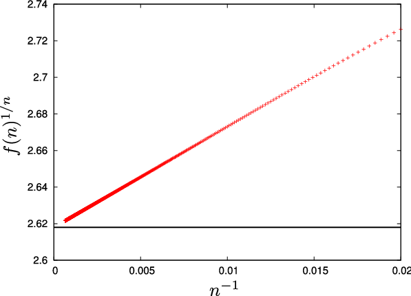
We have plotted the sequence of upper bounds, , together with the lower bound in Figure 9 (left). It is not unreasonable to extrapolate these upper bounds and reach the following conjecture:
Conjecture 11.
The growth rate of Thompson’s group with standard generating set is .
 |
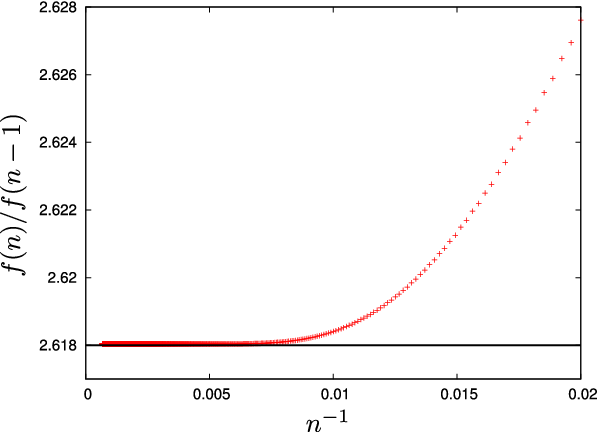 |
To further support this conjecture we have examined the sequence which must converge to the growth rate and we observe that it converges extremely rapidly to Guba’s lower bound. Additionally, in Figure 9 (right) we have plotted . The limit of this ratio, if it exists, must be the growth rate. While we have not been able to prove convergence it does appear to converge rapidly and is nearly indistinguishable from Guba’s bound. Note that Guba computed this ratio for in [16], to obtain a conjectured upper bound of .
Numerical analysis of the series [10] indicates that the corresponding generating function has an isolated simple pole at implying that
| (7) |
with . The first correction term appears to be approximately . We estimated this term by studying the asymptotics of the generating function ; this polynomial factor cancels the dominant contribution to the asymptotics from the (observed) simple pole at .
4 Outlook
In this paper we have described two algorithms for computing the size of the sphere of radius of Thompson’s group with standard generating set. The first of these runs in exponential time and polynomial space, is potentially generalisable to other groups, and also computes the geodesic growth series. The second runs in polynomial time and space and we have used it to compute the first 1500 terms of the growth series. We then used Fekete’s lemma to compute upper bounds for the growth rate from this data. This work suggests that the growth rate of is exactly equal to . This strongly indicates that the normal forms described in [15, 16] have very nearly geodesic length. More precisely, we believe that the word length of the normal form of a typical element differs from its geodesic length only by .
We analysed the sequence using our data and we have found some indication (using series analysis techniques such as differential approximants [17]) that the corresponding generating function contains square-root singularities and so is unlikely to be rational. Further, despite having the first fifteen hundred terms of the sequence, we have been unable to conjecture a rational, algebraic or differentiably finite generating function. In particular we used Guess package developed by Manuel Kauers [19] to search through a wide range of possible recurrences55 5 The sequence in question does not satisfy any homogeneous linear recurrence of order with polynomial coefficients of degree at most , where and and taken from the list . This is a roughly exhaustive search of the all such recurrences that can be detected with the first 1500 terms. Note that any rational, algebraic or differentiably finite sequence must also satisfy a homogeneous linear recurrence with polynomial coefficients.. Unfortunately this search did not find any candidates. While this does not prove that the generating function lies outside these classes, it does rule out the possibility that the generating function is simple (satisfying a recurrence of low degree or order).
It is relatively straightforward to extend Algorithm B to generate elements of a fixed geodesic length uniformly at random in polynomial time. Algorithm A was derived from an approximate enumeration algorithm [21] which can also be used to sample large elements of the group. We are currently investigating how these random generation techniques might be used (in the same spirit as [5]) to explore properties of the group that are still beyond analytic techniques such as its amenability.
References
- [1] J.M. Belk and K.S. Brown. Forest diagrams for elements of Thompson’s group . Internat. J. Algebra Comput., 15:815–850, 2005.
- [2] M. Bousquet-Mélou. A method for the enumeration of various classes of column-convex polygons. Disc. Math., 154(1-3):1–25, 1996.
- [3] M. Bousquet-Mélou and M. Petkovšek. Linear recurrences with constant coefficients: the multivariate case. Disc. Math. 225: 51–75, 2000.
- [4] M. Bousquet-Mélou and M. Petkovšek. Walks confined in a quadrant are not always D-finite. Theoret. Comput. Sci. 307: 257–276, 2003.
- [5] J. Burillo, S. Cleary, and B. Wiest. Computational explorations in Thompson’s group . In Geometric Group Theory, Geneva and Barcelona Conferences. Birkhauser, 2007.
- [6] J. W. Cannon, W. J. Floyd, and W. R. Parry. Introductory notes on Richard Thompson’s groups. Enseign. Math. (2), 42(3-4):215–256, 1996.
- [7] S. Cleary and J. Taback. Combinatorial properties of Thompson’s group . Trans. AMS., 356(7):2825–2849 (electronic), 2004.
- [8] A.R. Conway, A.J. Guttmann, and M. Delest. The number of three-choice polygons. Math. Comput. Modelling, 26:51–58, 1997.
- [9] M. Elder and A. Rechnitzer. Some geodesic problems for finitely generated groups. Arxiv preprint arXiv:09, 2009.
- [10] M. Elder, É. Fusy and A. Rechnitzer. Experimenting with Thompson’s group . In preparation – title subject to change.
- [11] I.G. Enting and A.J. Guttmann. Self-avoiding polygons on the square, L and Manhattan lattices. J. Phys. A: Math. Gen., 18(6):1007–1017, 1985.
- [12] S. Felsner, É. Fusy, M. Noy, and D. Orden. Bijections for Baxter Families and Related Objects. Arxiv preprint arXiv:0803.1546, 2008.
- [13] S.B. Fordham. Minimal Length Elements of Thompson’s Group . Geom. Dedicata, 99(1):179–220, 2003.
- [14] R. Grigorchuk and T. Smirnova-Nagnibeda. Complete growth functions of hyperbolic groups. Inven. Math., 130(1):159–188, 1997.
- [15] V.S. Guba and M.V. Sapir. The Dehn function and a regular set normal forms for R. Thompson’s group . J. Aust. Math. Soc. Series A, 62:315–328, 1997.
- [16] V.S. Guba. On the Properties of the Cayley Graph of Richard Thompson’s Group . Int. J. of Alg. Computation, 14(5-6):677–702, 2004.
- [17] A.J. Guttmann. Asymptotic analysis of power-series expansions. Phase Transitions and Critical Phenomena, 13:1–234, 1989.
- [18] J.M. Hammersley and K.W. Morton. Poor man’s Monte Carlo. J. Roy. Statist. Soc. B, 16(1):23–38, 1954.
- [19]
M. Kauers.
Guess — a Mathematica package for guessing multivariate and univariate
recurrence equations.
Available from
http://www.risc.uni-linz.ac.at/research/combinat/software/ - [20] F. Matucci. Algorithms and Classification in Groups of Piecewise-Linear Homeomorphisms. Arxiv preprint arXiv:0807.2871, 2008.
- [21] A. Rechnitzer and E.J. Janse van Rensburg. Fast Track Communication. J. Phys. A: Math. Theor., 41:442002, 2008.
- [22] M.N. Rosenbluth and A.W. Rosenbluth. Monte Carlo calculation of the average extension of molecular chains. J. Chem. Phys., 23(2):356–362, 1955.
- [23] N. J. A. Sloane. The On-Line Encyclopedia of Integer Sequences, (2008) http://www.research.att.com/njas/sequences/
- [24] R.P. Stanley. Enumerative Combinatorics: Volume 2. Cambridge University Press, 1999.
- [25] H.N.V. Temperley. Combinatorial Problems Suggested by the Statistical Mechanics of Domains and of Rubber-Like Molecules. Phys. Rev., 103(1):1–16, 1956.
- [26] J.H. van Lint and R.M. Wilson. A Course in Combinatorics. Cambridge University Press, 2001.
Appendix A Appendix: Pseudocode
Throughout the appending we will use the following notations:
- (i).
: set the variable to value ,
- (ii).
: the boolean operation that returns “true” if and are the same and otherwise returns “false”, and
- (iii).
: increment the variable by .
We use to distinguish the assignment of a value to a variable from the test for equality. While we could use instead of we feel that the later easier to read when using long and descriptive variable names.
A.1 Algorithm A
The function ComputeGeod recursively outputs all geodesic words of length .
Of course this function has the drawback that it generates a list of the geodesics that must be stored either in memory or on disk before it can be processed to give the number of elements. The following function avoids that problem.
Calling ComputeSphere(), where is the empty word, will return the size of the sphere of radius . It recursively computes the geodesics of length starting with prefix and instead of storing them in a list, it returns the sum of their contributions. Alternatively a non-recursive procedure NextGeodesic() is given below. This computes the first geodesic after of length at most .
A.2 Algorithm B
We give the pseudocode for our main algorithm divided into three different functions. Given the current state of the upper (or lower) forest diagram that is left of the pointer, the function UpdateLeft() returns the possible states of the diagrams produced by a valid transition (as described in Section 3.2 above). Similarly, given the current state of the upper (or lower) forest diagram that is right of the pointer, the function UpdateRight() returns the possible states of the diagrams produced by a valid transition.
Finally, CountForestDiagrams() enumerates all forest diagrams according to their weight (the geodesic length of the group elements they represent). It starts from the empty diagram with gaps labelled by . At each iteration it runs through all the pairs of upper and lower states that have been reached and determines which pairs of states can be reached by valid transitions using UpdateLeft() and UpdateRight(). The transitions of the upper and lower forests are nearly independent of each other; the only restriction is that we avoid creating common carets and they are easily avoided. The weight of the diagram can then be updated using the information in Table 1 and the appropriate counters can be updated. At the end of each iteration we output the number of completed diagrams of the current weight (which are those ending in gaps labelled .