Cosmological footprints of loop quantum gravity
Abstract
The primordial spectrum of cosmological tensor perturbations is considered as a possible probe of quantum gravity effects. Together with string theory, loop quantum gravity is one of the most promising frameworks to study quantum effects in the early universe. We show that the associated corrections should modify the potential seen by gravitational waves during the inflationary amplification. The resulting power spectrum should exhibit a characteristic tilt. This opens a new window for cosmological tests of quantum gravity.
Keywords:
Quantum gravity, quantum cosmologypacs
04.60.Pp, 04.60.Bc, 98.80.Cq, 98.80.QcPhys. Rev. Lett. 102, 081301 (2009)
Introduction- A fully convincing quantum theory of gravity is still missing. Beyond the internal
theoretical difficulties, experimental probes are extremely difficult to find. The two
main paradigms to investigate quantum gravitational effects are unquestionably string
theory and Loop Quantum Gravity (LQG). This latter approach is a promising way to
derive a background independent quantum theory of spacetime based only on the
experimentally well confirmed principles of general relativity (GR) and quantum mechanics.
Introductions can be found in Rovelli’s book [1] and Smolin’s review
article [2]. Based on the reformulation of GR as a kind of
gauge theory obtained by Sen [3] and Ashtekar [4] in the 1980’s,
LQG is now a language and a dynamical framework which leads to a mathematically
coherent description of the physics of quantum spacetime. Important problems are still
to be solved in LQG, starting with an explicit semi-classical limit recovering
GR, but the important results obtained both in black hole physics (see, e.g., [5]) and cosmology (see, e.g., [6]) urge an
experimental test of the theory. There are predictions for observable Planck scale
deviations from energy momentum relations [7] that lead to possibly measurable
effects for and very high energy gamma-ray experiments. Nothing
conclusive has however yet emerged from the associated analysis. In this article, we focus on
a new approach to search for observational probes of LQG [8]. It consists in investigating
into the details the way the amplification occurs during the inflationary phase when
taking into account the modified dispersion relation describing the propagation of
gravitons. First, the general framework is described together with the
Shrödinger-like equation of motion which encodes the LQG corrections in the potential
term. Then, the primordial tensor power spectrum is
explicitly derived and the tilt is given as a function of the LQG Barbero-Immirzi
parameter for a specific and favoured value of the parameter. Both de Sitter and
power-law inflations are considered. Finally, the validity of the overall scheme is
checked and a few points are made about possible developments.
Two basic types of quantum corrections are expected from the Hamiltonian of LQG. These corrections arise from inverse powers of the densitized triad and from the fact that loop quantization is based on holonomies, i.e. exponentials of the connection, rather than direct connection components. In the following article we focus on holonomy corrections as the inverse volume terms were found to exhibit a fiducial cell dependence and not to be adequate to describe models with a flat background [9]. Unlike studies based on the controversial superinflation scenario (see, e.g., [10]) we choose in this article to focus on a conservative approach where the background dynamics is supposed to be described by a standard de-Sitter or power-law inflation whereas the LQG terms act as corrections on the mode propagation. This picture is meaningful for at least two reasons. First, at the fundamental level, because it is highly probable [11] (although still questioned [12]) that superinflation cannot solve alone the problems of cosmology and should be considered as an appropriate way to set the initial conditions for the standard inflation. Our approach holds in this second phase. Then, at the heuristic level, because in such an intricate framework, it is very useful not to mix all the effects. A full LQG treatment of the cosmological evolution is not yet possible and the aim of this paper is to focus on a well determined effect. It was shown [13] that the propagation of gravitons in a FLRW universe is given, when holonomy corrections (which provide higher order and higher spatial derivative terms) are taken into account, by the following equation of motion:
| (1) |
where is the conformal time defined by is a parameter related to the action of the fundamental Hamiltonian on a lattice state that can be understood as the coordinate size of a loop whose holonomy is used to quantize the Ashtekar curvature components, is so that depends on the triad component through , and is the Barbero-Immirzi parameter. The right-hand side of this differential equation corresponds to the source term of gravitational radiations. It also receives corrections from holonomies and vanishes in the absence of matter. The friction term and the last term of the left-hand side are given by the background evolution, as solved in the LQG framework. One can then compute the equation of motion for tensor perturbation modes with , . The value of depends on the scheme adopted to quantize holonomies. Furthermore [13], and has to be chosen so that has the dimension of a length. The exact value of and its dependence upon are still under debate. For the specific case , it was shown [5] that and it seems quite natural to phenomenologically parametrize by Using Eq. (29) to (31) from Bojowald & Hossain [13], the equation of motion (1) can be re-written as a function of the cosmological parameters (the scale factor and the energy density of the background ) and of three LQG parameters (, and ):
| (2) |
where we have replace by and . Introducing a new field , Eq. (2) now reads:
| (3) |
where is the second derivative according to the conformal time . Decomposing the field into its spatial Fourier modes, and using the standard Friedmann equation relating the Hubble constant to the energy density of the background, one has to deal with the following equation:
| (4) |
It should be underlined that strictly speaking the tree-level Friedman equation in LQG reads as
| (5) |
where in [9]. Our whole approach consistently assumes .
Eq. (4) is easily interpreted if one remembers the dynamical equation for gravitons in a FLRW background without LQG corrections:
with the source term in GR. Holonomy corrections
appear as a modification of the dispersion relation. This modification is
encoded in the last term of the left-hand side of Eq. (3) and depends on the
dynamics of the universe through the scale factor, on its content through the
energy density of the background and on the LQG parameters. It can also be
noticed that, in addition to its time dependence through the scale factor, the
correction term scales, as expected, as
This equation can be interpreted as a Schrödinger equation, being the energy
and being the
potential . In GR, the potential is simply given by .
Power spectra- To derive explicitly the power spectrum, we focus on the case . There is a lively debate within the LQG community between two versions of the theory and we begin by considering the Ashtekar, Pawlowski and Singh scheme. In this approach, the choice is necessary (see, e.g., [14]) to ensure that the theory is independent on arbitrary background structures introduced in the process of quantization. As we deal with the amplification of vacuum quantum fluctuations, the source term in Eq. (4) is set to zero. For a de Sitter (dS) inflation, the scale factor is given by with . Therefore, the equation of motion for gravitons
can be solved by a Linear Combination (LC) of Hankel functions 11 1 We choose the Hankel functions as the basis for the solution as they satisfy the correct Wronskian condition for a standard particle interpretation of quantum field theory.:
| (6) |
and being two constants of integration determined by the initial conditions found by studying the region where the adiabatic vacuum can be defined (see, e.g., [15]). In this so-called Bunch-Davies vacuum, the solutions are plane waves
| (7) |
whose matching with the previously given general solution allows to determine and . The choice of the vacuum is clearly a non-trivial question in this framework. However, to remain consistent with our hypothesis, we assume the de-Sitter background to be a correct approximation from the beginning of inflation. In this case, the appropriate conditions will inevitably be met in the remote past , i.e. when . This will not be true anymore when considering inverse volume corrections [16]. Finally, the solution is expanded around the high amplification regime, which leads to the following power spectrum, defined as (using the convention of [15]):
| (8) |
It can be seen that LQG corrections do not only modify the normalization of the spectrum but also, and more importantly, lead to a departure from scale invariance. The tensor index is given by:
| (9) |
which shows that the spectrum becomes blue for a real-valued Barbero-Immirzi parameter (which is the more realistic case, as inferred, e.g., from the entropy of black holes) and red if is imaginary. This can be easily understood at the intuitive level. The amplification starts at the critical time . If this is later than in the standard general relativistic case and modes are therefore less amplified. As the difference between the value of with LQG corrections and without LQG corrections becomes smaller as increases, short wavelengths will undergo a smaller suppression. The spectrum will therefore be blue.

Several cases can be investigated into more details. First, it is worth considering a power-law inflation. For this inflationary model, the scale factor is given by , with . Using , where , the potential term now reads
| (10) |
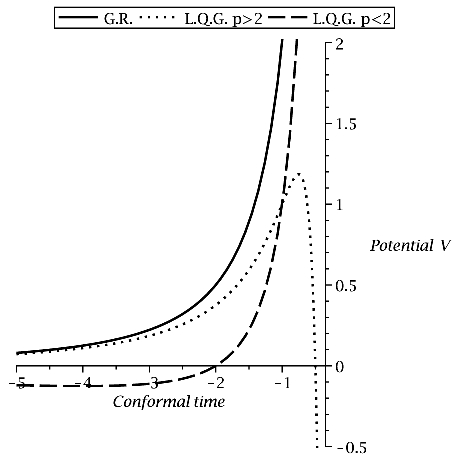
Because , the LQG corrections dominate at the beginning of inflation and become negligible at the end. Moreover, it can be seen from Fig. 2 that adding LQG corrections lowers the effective potential. As the amplification occurs when , it is obvious from a simple WKB reasoning that high -modes will not be much affected by LQG corrections whereas low -modes will be less amplified than in the standard power-law case. LQG corrections being subdominant at the end of inflation, the mode functions are still well approximated by a LC of Hankel functions like in Eq. (6) with . The primordial power spectrum is then given as a function of and by taking the asymptotic expansion of the Hankel functions:
| (11) |
With the considered potential, the equation of motion for gravitons cannot be solved analytically, though the asymptotic limits can be found. Because the LQG term is subdominant at the end of inflation, the amplification is effective only in the UV regime (i.e. ) and the power spectrum should be approximated by the standard prediction of power-law inflation for high values of the wavenumber. This leads to
| (12) |
Then, it is possible to compute the spectrum in the IR limit (i.e. ). The dependant solution given in Eq. (6), valid at the end of inflation, is matched to a solution valid during the entire inflationnary era, but only for . By setting and with the change of variables , , the equation of motion takes the form of a Bessel equation. This allows us to find a solution for the -modes function, valid throughout the whole inflationary era, as a LC of Hankel functions. The coefficients of this solution are found requiring the Wronskian to be equal to 22 2 The standard requirement in field theory is that the Wronskian should be equal to . However, is already a rescaled quantity and the Wronskian condition now reads . This is in agreement with the convention of Martin & Schwarz and with the normalization of the Bunch-Davies vacuum we used to derive the power spectrum for dS inflation.:
| (13) |
with . Finally, the matching between the two solutions is performed at the end of inflation by taking the asymptotic limit of the solution of (6) when and the one of solution (13) when . This leads to:
| (14) |
This allows us to derive the primordial power spectrum in the IR and UV regimes:
| (15) | |||||
| (16) |
In both regimes, the power spectrum is well described by a power-law with a red (blue) spectrum in the UV (IR) region. To compute the power spectrum throughout the entire range of wavenumbers, the differential equation has been numerically solved with the Bunch-Davies vacuum as initial conditions. The results are displayed on Fig. 1. This shows the very good agreement between the numerical computation and the UV and IR approximations. The value of was deliberately chosen very small to make the reading easier. As the UV approximation is also the primordial spectrum obtained without LQG corrections, it can be seen that adding the LQG correction term leads to a suppression of the long wavelength perturbations as compared to the prediction of GR.
The results obtained in the power-law inflation framework can be directly applied to slow-roll inflation, which is a realistic scenario in agreement with WMAP data. In particular, the asymptotic expansions of Eqs. (15) and (16) are still valid with the appropriate replacement of by 33 3 In the slow-roll approximation, the scale factor is approximated by at the horizon crossing.. This leads to:
| (17) |
where has been expressed as a function of and , respectively the conformal
time and Hubble constant at horizon crossing . A Taylor expansion in has
also been performed.
Prospects and validity of the approach- In the Ashtekar, Pawlowski and Singh approach considered so far, must be equal to -1/2. However, Bojowald has criticized this conclusion (see, e.g., [19] for a very recent discussion) and, for the completeness of our conclusions, it worth investigating the case at the qualitative level. For the three inflationary models studied in this article (dS, power-law and slow-roll), the potential reads as , where are positive constants such that and . Depending on the values of and , the exponent of the LQG correction terms is either smaller or greater than 2. (When , is always smaller than 2). The shape of the potential is displayed on Fig. 2 together with the GR potential. The case (dashed line) was studied in the previous section, where numerical investigations confirmed the naïve WKB-based idea that amplification is less effective in the IR regime while roughly the same than in GR in the UV regime. The situation drastically differs when (dotted line) as the LQG term now dominates at the end of inflation (this leads to the drop of the potential when ). With the same WKB reasoning, it is clear that the amplification is now less effective for high values of . Moreover, because the potential admits a maximum, the amplification totally disappears for . Finally, as the potential becomes negative valued, the mode functions can start to re-oscillate at the very end of inflation. This fundamentally changes the standard picture of the generation of perturbations as the temporal coherence of the two-point correlation function is restored before the transition from inflation to the radiation-dominated era. Even with very close to -2, as expected from WMAP data [17], this can happen for slightly above -1/2.
It is well known that a complete description of the primordial fluctuations amplified during inflation requires, in principle, to derive the full quantum statistical properties of the Bunch-Davies vacuum (the in vacuum) in terms of quanta defined in the radiation-dominated era (the out quanta). In the standard GR case, the quantum statistical distribution is maximally coherent due to the high enough amplification of quantum fluctuations (i.e. when ). This high level of coherence ensures the classical description to be a good approximation at the level of power spectra. In other words tensor fluctuations can be described by a classical, Gaussian distribution with zero mean and a variance proportional to the power spectrum (see [18] for a detailed discussion of the link between the apparent classicality and the coherence of the quantum distribution). When LQG corrections are considered, the above statement still holds when simply because LQG corrections are negligible at the end of inflation. When , LQG correction are now dominant at the end of inflation and a complete analysis is needed. For super-horizon modes, an asymptotic solution in terms of Bessel functions of the field equation can be found, allowing us to explicitly compute the Bogoliubov coefficients relating the in vacuum to the out quanta. In the limit , the two Bogoliubov coefficients are related one to the other by
| (18) |
Because , the above-mentioned relation ensures that the distribution is
maximally coherent and the classical description is still a good approximation. In
other words, the classical description valid in a general relativistic framework still
holds when LQG settings are considered if inflation lasts long enough.
Conclusion- Testing quantum theories of gravity is probably one of the most important challenge of current fundamental physics. Loop Quantum Gravity has not yet been experimentally probed but it seems that cosmological observations could allow for a clear signature of LQG effects. This article opens a new window on quantum gravity by suggesting a way to possibly observe holonomy corrections. Although B-mode detection could be achieved by the Planck satellite and is the main goal of several dedicated experiments for the forthcoming decade, the signal remains very difficult to extract from the lensing background and some further refinements are required to quantify the amplitude of the expected LQG effects. Furthermore, string gaz cosmology also predicts a deviation from scale-invariance [20] and the discriminating criteria should be found. Most importantly, the formalism established in this article should be used for LQG corrections to scalar perturbations that are just being investigated [21] and could be even more promising from the observational viewpoint.
References
- [1] C. Rovelli, Quantum Gravity, Cambridge, Cambridge University Press, 2004
- [2] L. Smolin, arXiv:hep-th/0408048v3
- [3] A. Sen, J. Math. Phys. 22 1781 (1981)
- [4] A. Ashtekar, Phys. Rev. Lett. 57 2244 (1986)
- [5] A. Ashtekar & M. Bojowald, Class. Quantum Grav. 22 3349 (2005)
- [6] A. Ashtekar, M. Bojowald & J. Lewandowki, Adv. Ther. Math. Phys. 7 233 (2003)
- [7] J. alfaro, H.A. Morales-Tcotl & L.F. Urrutia, Phys. Rev. D 65 103509 (2002)
- [8] A. Barrau & J. Grain, Proc. of the 43rd ”Rencontres de Moriond” Cosmology-2008, arXiv:0805.0356v1 [gr-qc]
- [9] A. Ashtekar, T. Pawlowski & P. Singh, Phys. Rev. D 74 084003 (2006)
- [10] J. Mielczarek, arXiv:0807.0712v1
- [11] S. Tsujikawa, P. Singh & R. Maartens, Class. Quant. Grav. 21 (2004) 5767
- [12] E.J. Copeland et al., Phys. Rev. D 77 (2008) 023510
- [13] M. Bojowald & G. M. Hossain, Phys. Rev. D 77 023508 (2007)
- [14] A. Corichi & P. Singh, Phys. Rev. D 78 024034 (2008)
- [15] J. Martin, Lect. Notes Phys. 738 193 (2008); J. Martin & D. Schwarz, Phys. Rev. D 62 103520 (2000); Phys. Rev. D 67 083512 (2003)
- [16] J. Grain, A. Barrau & A. Gorecki, arXiv:0902.3605v1
- [17] E. Komatsu et al., arXiv:0803.0547v2
- [18] Polarski & A. A. Starobinsky, Class. Quant. Grav. 13 377 (1996); D. Campo & R. Parentani, Phys. Rev. D 72 045015 (2005); Phys. Rev. D 74 025001 (2006)
- [19] M. Bojowald, arXiv:0811.4129v1
- [20] R.H. Brandenberger, A. Nayeri, S.P. Patil & C. Vafa, Phys. Rev. Lett 98 231302 (2007)
- [21] M. Bojowald, G. Hossain, M. Kagan & S. Shankaranarayanan, arXiv:0811.1572