Mortar Boundary Elements
Abstract
We establish a mortar boundary element scheme for hypersingular boundary integral equations representing elliptic boundary value problems in three dimensions. We prove almost quasi-optimal convergence of the scheme in broken Sobolev norms of order . Sub-domain decompositions can be geometrically non-conforming and meshes must be quasi-uniform only on sub-domains. Numerical results confirm the theory.
Key words: boundary element method, domain decomposition, mortar method, non-conforming Galerkin method
AMS Subject Classification: 65N55, 65N38
1 Introduction and model problem
In the finite element framework, mortar methods are used to discretize a given problem independently on sub-domains. It is a non-overlapping domain decomposition method. Necessary continuity requirements on interfaces of the sub-domains are implemented via Lagrangian multipliers. The motivation is to facilitate the construction of finite element meshes on complicated domains and to allow for parallelization. Bernardi, Maday and Patera introduced this technique and gave first analyses in [3, 4]. Later, geometrically non-conforming sub-domain decompositions and problems in have been studied by Ben Belgacem and Maday [2, 1]. There is a large number of publications on mortar methods, all dealing with the discretization of differential equations of different types and with related numerical linear algebra. The first papers, just mentioned, derive a priori error estimates in the framework of non-conforming methods involving a Strang type estimate.
In this paper we establish a mortar setting for the boundary element method (BEM) and prove almost quasi-optimal convergence for a model problem involving the hypersingular operator of the Laplacian. The advantages of this domain decomposition scheme (easier construction of meshes and availability of parallel techniques) also apply to the BEM. To be precise, we apply the mortar technique directly to the boundary element discretization, not as a coupling procedure between boundary and finite elements as in [9]. The analysis of finite elements for the discretization of boundary integral equations of the first kind goes back to Nédélec and Planchard [21], and Hsiao and Wendland [17]. Stephan [22] studied boundary elements for singular problems on open surfaces. Hypersingular boundary integral equations are well posed in fractional Sobolev spaces of order and conforming Galerkin discretizations require continuous basis functions. Due to the non-existence of a trace operator in these Sobolev spaces, needed for the analysis of interface conditions, mortar boundary elements give rise to a variational crime. Indeed, it turns out that there is no well-defined continuous variational formulation of the mortar setting for the BEM. Instead we will analyze the discrete mortar scheme as a non-conforming method for the original un-decomposed integral equation. We follow the analysis presented in [1] where projection and extension operators are used to bound the approximation error in the kernel space (of functions satisfying the Lagrangian multiplier condition). Note that there is a shorter presentation by Braess, Dahmen and Wiener [7] where the simpler argument [6, Remark III.4.6] is used to bound this error by a standard approximation error (in un-restricted spaces). Nevertheless, in our case the Strang type error estimate has a more complicated structure and it is not straightforward to follow the argument [6, Remark III.4.6].
We will make use of some preliminary results in [13, 16]. In [13] we studied the discretization of hypersingular operators on open surfaces using functions that vanish only in a discrete weak sense on the boundary of the surface. Such functions in general do not belong to the energy space of the operator and require a different variational setting. This setting will be used also for the mortar boundary elements. In [16] this setting served to establish (non-conforming) Crouzeix-Raviart boundary elements and to prove their quasi-optimal convergence. Main tool in that paper is a discrete fractional-order Poincaré-Friedrichs inequality. It serves to show ellipticity of the principal bilinear form of the discrete scheme. In this paper we generalize this inequality to the geometrically non-conforming case, needed for general mortar decompositions. Again, it is needed to prove (quasi-) ellipticity of the principal bilinear form. Our model problem is defined on an open flat surface with polygonal boundary. We prove that, up to logarithmical terms, the mortar boundary element method converges quasi-optimally, subject to a compatibility condition of the boundary meshes and the meshes on the interfaces for the Lagrangian multipliers. Here we rely on the known Sobolev regularity of the exact solution leading to almost -convergence where is the maximum mesh size. Our techniques are applicable also to polyhedral surfaces and include meshes of shape-regular triangles and quadrilaterals.
An overview of this paper is as follows. In the rest of this section we recall definitions of fractional order Sobolev norms and formulate the model problem. In Section 2 we define the mortar scheme and present the main result (Theorem 2.1) establishing almost quasi-optimal convergence of the mortar boundary element method. Technical details and proofs are given in Section 3. In Section 4 we present some numerical results that underline the stated convergence of the mortar BEM.
First let us briefly define the needed Sobolev spaces. We consider standard Sobolev spaces where the following norms are used: For a bounded domain and we define
with semi-norm
For the space is defined as the completion of under the norm
For , and are equivalent norms whereas for there holds , the latter space being the completion of with norm in . Also we note that functions from are continuously extendable by zero onto a larger domain. For details see, e.g., [18, 14]. For , the spaces and are the dual spaces of and , respectively.
Let be a plane open surface with polygonal boundary. In the following we will identify with a domain in , thus referring to sub-domains of rather than sub-surfaces. The boundary of is denoted by .
Our model problem is: For a given find such that
| (1.1) |
Here, is a normal unit vector on , e.g. . We note that maps continuously onto (see [23]). We have the following weak formulation of (1.1). Find such that
| (1.2) |
Here, denotes the duality pairing between and . Throughout, this generic notation will be used for other dualities as well, the domain mentioned by the index.
A standard boundary element method (BEM) for the approximate solution of (1.2) is to select a piecewise polynomial subspace and to define an approximant by
Such a scheme is known to converge quasi-optimally in the energy norm, cf. Remark 2.1 below. In the numerical section we will compare such a conforming approximation with a mortar approximation, for the case where the meshes are globally conforming.
2 Mortar method and main result
In this section we introduce the mortar boundary element method for the approximate solution of the model problem (1.2). First we discuss the decomposition of into sub-domains. Then we introduce the discrete approximation spaces. The main result of this paper is given at the end of this section.
2.1 Sub-domain decomposition
We consider a decomposition of into non-intersecting sub-domains , , giving rise to a coarse mesh
For ease of presentation we assume that each is either a triangle or quadrilateral. More general decompositions into polygonal sub-domains can be dealt with by further decomposing into triangles and quadrilaterals and by considering conforming interface conditions on additional interfaces. The mesh can be non-conforming but must satisfy the assumption (A1) below. The diameter of a sub-domain is denoted by , and The interface between two neighboring sub-domains , (, contains more than a point) is denoted by . For our analysis below we need the following assumption.
(A1) Each interface consists of an entire edge of or .
The (relatively) open edges of a sub-domain are , . Here, is a generic number ( if is a triangle and otherwise). Using the symbol for the boundary of , and similarly for the boundary of , the skeleton of the sub-domain decomposition is
According to assumption (A1) the skeleton is covered by a set of non-intersecting edges . We number the edges like , …, , giving a decomposition of the skeleton like In the following we will denote this decomposition of the skeleton by
We will refer to these edges as interface edges. Each interface edge is the interface between two sub-domains , and is an entire edge of one or both of them. Given an integer () we denote by (respectively, ) the number of a sub-domain which has as an edge (respectively, the number of the other sub-domain),
As mentioned before, the selection of the index pair for is not unique but will be fixed for a specific sub-domain decomposition of . Below, we will introduce a Lagrangian multiplier on the interfaces and on we will use a mesh related to the mesh on . The side of stemming from is usually called mortar side in the finite element literature and this explains our notation. The side defining the Lagrangian multiplier is often called non-mortar side.
Corresponding to the decomposition of we will need the product Sobolev space
with usual product norm.
2.2 Meshes and discrete spaces
On each of the sub-domains () we consider a (sequence of) regular, quasi-uniform meshes consisting of shape regular triangles or quadrilaterals, . The maximum diameter of the elements of is denoted by and we use the symbols
Throughout the paper we assume without loss of generality that . This makes the writing of logarithmic terms in easier.
In the case of being a square, Figure 2.1 shows a conforming sub-domain decomposition (a) and a non-conforming sub-domain decomposition (b), both with globally non-conforming meshes.

Now we introduce discrete spaces on sub-domains consisting of piecewise (bi)linear functions,
The global discrete space on is
Note that functions do satisfy the homogeneous boundary condition along but are in general discontinuous across interfaces. Therefore, is not a subspace of the energy space . Functions from different sub-domains will be coupled via a discrete Lagrangian multiplier on the skeleton. To this end we introduce a mesh on the skeleton as follows.
On each interface edge there is a trace mesh inherited from the mesh on the sub-domain . (We recall that by definition, is an entire edge of the sub-domain with number .) This trace mesh is quasi-uniform with mesh width . Now we introduce a new (coarser) quasi-uniform mesh on in such a way that the following assumption is satisfied.
(A2) For any there holds: the mesh is a strict coarsening of the trace mesh . In particular, any interior node of together with its two neighboring elements (intervals) is covered by one element of .
The mesh width (length of longest element) of is denoted by , and On each interface edge we define a space of piecewise constant functions,
The space for the discrete Lagrangian multiplier then is
Notations. The symbols “” and “” will be used in the usual sense. In short, when there exists a constant independent of the discretization parameter and the involved function such that for any of the given set. The double inequality is simplified to . The generic constant above is usually also independent of appearing fractional Sobolev indexes , but this will be mentioned. We note that these notations usually do not mean independence of involved constants on the decomposition of . In this paper we consider a generic decomposition which is fixed and estimates will in general depend on .
Throughout the paper we also will use the notation for the restriction of a function to the sub-domain .
2.3 Setting of the mortar boundary element method and main result
For the setup of the mortar boundary element method we need some operators. We introduce the surface differential operators
The definitions of the surface curl operators are appropriate just for flat surfaces (as in our case) but can be extended to open and closed Lipschitz surfaces, cf. [8, 13]. We define corresponding piecewise differential operators and by
The notations and refer to the restrictions of and , respectively, onto , and indicates extension by zero to . We made use of the notation introduced before, , . Furthermore, we need the single layer potential operator defined by
For the formulation of the mortar boundary element method we define, for sufficiently smooth functions , , , the bilinear forms and by
Here, as mentioned before, for a domain or an arc , denotes the -inner product and its extension by duality, and is the jump of across , more precisely
Of course, for sufficiently smooth functions , , there holds
Note that we will use the introduced notations and for duality pairings of product spaces corresponding to the given decompositions ( and ). We also define, for a sufficiently smooth function , the linear form
where is the function given in (1.1). The mortar boundary element method for the approximate solution of (1.2) then reads: Find and such that
This scheme is equivalent to: Find such that
where
| (2.4) |
The main result of this paper is as follows.
Theorem 2.1.
There exists a unique solution of (2.3). Assume that the solution of (1.2) satisfies (). Then there holds
For proportional mesh sizes and this means that
The appearing constants in the estimates above are independent of and provided that the assumptions on the meshes, in particular (A1) and (A2), are satisfied.
A proof of this theorem is given at the end of Section 3.
Remark 2.1.
As in [13] we note that, in our case of an open surface , the solution of (1.1) has strong corner and corner-edge singularities which cannot be exactly described by standard Sobolev regularity. It is well known that for any (see, e.g., [24]) so that the error estimate by Theorem 2.1 holds for any . In general but a more specific error analysis for the conforming BEM yields for quasi-uniform meshes the optimal error estimate
see [5]. The logarithmical perturbations in of our error estimate are due to the non-conformity of the mortar method. They stem from the non-existence of a trace operator within and from non-local properties of the fractional order Sobolev norms (the difference between and -spaces).
3 Technical details and proof of the main result
We start by citing some technical results (Lemmas 3.1-3.4) which are needed to deal with the fractional order Sobolev norms. Afterwards we study a discrete Poincaré-Friedrichs inequality (Proposition 3.1) which will be applied to prove ellipticity of the bilinear form on . Afterwards an integration-by-parts formula for the hypersingular operator is recalled from [13] and adapted to our situation of many sub-domains. Then, Lemma 3.5 states the well-posedness of integration by parts. Lemmas 3.6-3.13 study requirements for the Babuška-Brezzi theory and provide details for a Strang-type error estimate which is given by Theorem 3.1. Later, Lemmas 3.14 and 3.15 are needed to analyze the bound of the Strang-type estimate and lead to Theorem 3.2 which gives a general a priori error estimate for the mortar BEM. The section is finished by giving a proof of the main result (Theorem 2.1).
Lemma 3.1.
[15, Lemma 5] Let be a Lipschitz domain. There exists such that
Lemma 3.2.
Let be a Lipschitz domain, and let be a piecewise linear function defined on a quasi-uniform mesh on with mesh size . There exists a constant which is independent of (but may depend on ) such that there holds
Proof.
By [15, Lemma 6] there holds for a piecewise polynomial function of degree the estimate
Fixing gives the claimed bound. The proof of [15, Lemma 6] gives full details for rectangular meshes. For triangular meshes the proof applies as well by making use of Schmidt’s inequality for triangles, cf. [11, Lemma 5.1]. Nevertheless, we are considering only polynomials of low degrees where Schmidt’s inequality is not needed. ∎
Lemma 3.3.
[13, Lemma 4.3] Let be a bounded Lipschitz domain. There exists such that, for any , there holds
Here is the boundary of .
Lemma 3.4.
For being one of the sub-domains or there holds
| (3.1) |
The restriction of onto is continuous,
| (3.2) |
Moreover, there holds the continuity
| (3.3) |
Proof.
The following result is a generalized version of a discrete Poincaré-Friedrichs inequality in fractional order Sobolev spaces, cf. Theorem 8 in [16].
Proposition 3.1.
There exists a constant , independent of the decomposition as long as sub-domains are shape-regular, such that for all there holds
Here, denotes the length of .
Proof.
For the case of conforming decompositions of into triangles, [16, Theorem 8] proves that there holds
| (3.4) |
It is easy to see that the mean zero term can be avoided by assuming the homogeneous boundary condition for . To obtain the result for our non-conforming decomposition including quadrilaterals we introduce further edges to reduce quadrilateral sub-domains to triangles and to transform into a conforming decomposition . By definition of the Sobolev-Slobodeckij semi-norm there holds
We note that for new edges there holds by the trace theorem and the regularity for any . The result then follows from (3.4). ∎
Following [13] we now examine an integration-by-parts formula for the hypersingular operator. For a smooth scalar function and a smooth tangential vector field , integration by parts gives
Here, is the unit tangential vector on (oriented mathematically positive when identifying with a subset of which is compatible with the identification of as a subset of ). Applying this formula to , we obtain for smooth functions and
Now we sum over and take into account that on . Further we let , use the convention for the jump denote by the unit tangential vector along (again mathematically positive oriented) and let (remember the notation and for the numbers of the Lagrangian multiplier side and mortar side of , respectively). This yields
for a piecewise (with respect to ) smooth function on with , as defined before. In the last step we used the fact that
which holds by a density argument and the continuity of as the adjoint operator of , cf. (3.2).
Now we use the relation
see [19, 20] and [13, Lemma 2.3]. Then choosing a piecewise smooth function with we obtain
| (3.5) |
Here, denotes our Lagrangian multiplier on the skeleton defined by
| (3.6) |
Relation (3.5) does not extend to since the trace of such a function onto is not well defined. However, there holds the following lemma.
Lemma 3.5.
For with , (3.5) defines for any .
Remark 3.1.
The above lemma can be extended to values of larger than . Though small values of represent the interesting cases, the limit being excluded. Also, the condition on can be relaxed but excluding the case which is the standard regularity using the mapping properties of the hypersingular operator.
Proof of Lemma 3.5. We must show that defined by (3.5) is a bounded linear functional on , the dual space of .
Let be given. We continuously extend to an element with on such that . (Simply extend on each interface edge to a function in vanishing on and extend by zero to the rest of . Then sum up with respect to .) The definition of is independent of the particular extension , see [13] for details in the case of one sub-domain. Using a duality estimate we obtain from (3.5)
| (3.7) | |||||
Now, for the norms in and are equivalent (cf., e.g., [18]) so that together with the mapping property of [10],
and (3.2) we obtain
Here, the appearing constants are independent of but may depend on . Also, using (3.3) we are able to bound (with constant independent of )
Taking the last two estimates into account, (3.7) proves that
Using the continuity of the extension (with constant independent of )
finishes the proof. ∎
Lemma 3.6.
Proof.
By (3.1) there holds
| (3.8) |
For there holds for any interface edge since by construction contains the piecewise constant function which has the value on and vanishes on . For the definition of (the discrete kernel of ) see (2.4). Therefore, Proposition 3.1 proves that
Here, the appearing constant is independent of . Making use of the inverse property we bound
so that, with the previous estimate,
| (3.9) |
Selecting (for being small enough) and combining (3.9) with (3.8) proves the statement. ∎
Lemma 3.7.
The bilinear form is almost uniformly -elliptic. More precisely there hold the lower bounds
and
| (3.10) |
Proof.
Lemma 3.8.
The bilinear form is almost uniformly continuous on . More precisely there holds
Proof.
For the eventual error estimate we need the boundedness of the bilinear form . However, Lemma 3.8 is not applicable to non-discrete functions. Instead we will use the next lemma.
Lemma 3.9.
Assume that (). Then there holds
In particular, the appearing constant is independent of .
Proof.
In order to analyze the error bound of the Strang-type estimate by Theorem 3.1 below, we need to extend functions from interface edges to sub-domains. This is also required to prove an inf-sup condition for the bilinear form .
To this end let us define extension operators that extend piecewise linear functions from interface edges to piecewise (bi)linear functions on the corresponding Lagrangian sub-domain,
| (3.12) |
Here, for the extension is defined as the function of that coincides with in the nodes on stemming from the mesh and is zero in the remaining nodes of .
Lemma 3.10.
In particular, the appearing constant is independent of .
Proof.
Using the equivalence of norms in finite dimensional spaces and scaling properties of the -norm one obtains, by taking into account the construction of ,
Analogously we find
The result then follows by interpolation. ∎
Lemma 3.11.
The bilinear form satisfies the discrete inf-sup condition
Here, the constant is independent of and subject to the assumptions made on the meshes.
Proof.
Let be given. On each interface edge , is a piecewise constant function on , a mesh that is coarser than the trace mesh stemming from the Lagrangian side , cf. assumption (A2). On we construct a piecewise linear function in the following way. For each element , vanishes at the endpoints of , coincides with at one interior node of and is linearly interpolated elsewhere on . See Figure 3.1 for an example where is represented by the dashed line and by the solid line. The bullets indicate the nodes of the mesh for the Lagrangian multiplier and the dashes indicate additional nodes of the trace mesh (from the Lagrangian multiplier side).
We then extend to in by first extending to , cf. (3.12), and then further by zero onto . Eventually we define .
Note that vanishes on all interface edges except . The trace of onto from equals whereas the trace coming from the other side vanishes. This yields
| (3.13) |
By the construction of there holds, uniformly for ,
| (3.14) |
Also, taking into account that each sub-domain has a limited number of (interface) edges, determined by the relation , Lemma 3.10 yields
| (3.15) | |||||
Now, using (3.13), (3.14) and (3.15), we finish the proof by bounding
∎

Lemma 3.12.
Proof.
By the triangle inequality and Lemma 3.3 there holds uniformly for
The inverse property, applied separately to , yields
and selecting (for being small enough) finishes the proof. ∎
Lemma 3.13.
The bilinear form is almost uniformly discretely continuous, in the sense that
| (3.16) |
Moreover, for given , there holds
| (3.17) |
Proof.
We are now ready to prove the following Strang-type error estimate.
Theorem 3.1.
Proof.
The existence and uniqueness of follows from the Babuška-Brezzi theory. Indeed, the bilinear form is continuous on by Lemma 3.8 and -elliptic by Lemma 3.7, and the bilinear form is continuous on by (3.16) and satisfies a discrete inf-sup condition by Lemma 3.11. The continuity and ellipticity bounds depend on but that does not influence the unique solvability of the discrete scheme.
In order to analyze the upper bound provided by Theorem 3.1 we need, apart from the extension operators defined before, projection operators acting on and mapping onto special continuous, piecewise linear functions on , . We recall that on each we have two meshes: the trace mesh stemming from the mesh on the sub-domain of the Lagrangian side, and the mesh for the Lagrangian multiplier. For each element we consider a hat function that vanishes at the endpoints of and has the tip at a node of that is interior to . This choice is not unique if contains more than two elements of the trace mesh. In that case we select an arbitrary but fixed node for the definition of . Using this notation we define
| (3.19) |
such that the integral mean zero conditions
hold. This operator satisfies the following properties.
Lemma 3.14.
For any , vanishes at the endpoints of , , and there holds
| (3.20) |
| (3.21) |
Proof.
For let be given. By definition of , vanishes at the endpoints of , and the orthogonality (3.20) follows by noting that any is constant on any .
To show (3.21) let be given. With being the hat function defined previously (with height ) there holds
so that
Summing over finishes the proof. ∎
We are now ready to analyze the first term of the upper bound provided by Theorem 3.1.
Lemma 3.15.
For let . There holds
uniformly for .
Proof.
Let be given. We adapt such that the new function satisfies the jump conditions defining , cf. (2.4). We set
with
Here, and are the extension and projection operators specified in (3.12) and (3.19), respectively. Note that, since vanishes at the endpoints of , the extension vanishes on . Therefore, using (3.20) one obtains
That is, . We start bounding the error by
| (3.22) | |||||
Applying Lemma 3.10, (3.21) and the triangle inequality we find that there holds
| (3.23) | |||||
The next result provides an a priori error estimate for the mortar BEM.
Theorem 3.2.
Proof.
Since there holds
To this end note that (combine (3.2) with the continuity ) and . The trace theorem concludes the claimed regularity of . In particular there holds .
Proof of Theorem 2.1. By Theorem 3.1, system (2.3) is uniquely solvable. We employ the general a priori estimate by Theorem 3.2 to show the given error bound. By standard approximation theory there exist and such that
and as in the proof of Theorem 3.2 one concludes that . By Lemma 3.3 one bounds
and accordingly the mortar part . Using these bounds in Theorem 3.2 and selecting one obtains the assertion. ∎
4 Numerical results
We consider the model problem (1.2) with and . In this case there holds for any so that by Theorem 2.1 we expect a convergence of the mortar method close to , the convergence of the conforming BEM, cf. Remark 2.1. This assumes that the mesh sizes (of the sub-domain meshes) and (of the meshes for the Lagrangian multiplier on the skeleton) are proportional, which will be the case in all our experiments. In fact, the elements of the mesh for the Lagrangian multiplier will always consist of two or three elements of the trace mesh.
Since the exact solution to (1.1) is unknown we approximate an upper bound for the semi-norm . Here, we follow the strategy from [13]. Let us recall the procedure and discussion.
By the ellipticity of and (3.8) there holds
| (4.1) |
On the other hand, using that solves (1.1) and solves (2.3), one finds
By (3.5) there holds
such that, with the previous relation,
| (4.2) |
Like in the proof of Theorem 3.2 one sees that is bounded. Therefore, by (4.1) we find that
The terms and are directly accessible and can be approximated by an extrapolated value that we denote by (cf. [12]). Therefore, instead of the relative error
we present results for the expression
| (4.3) |
which is, up to a constant factor, an upper bound for .
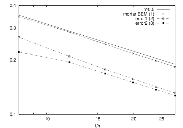
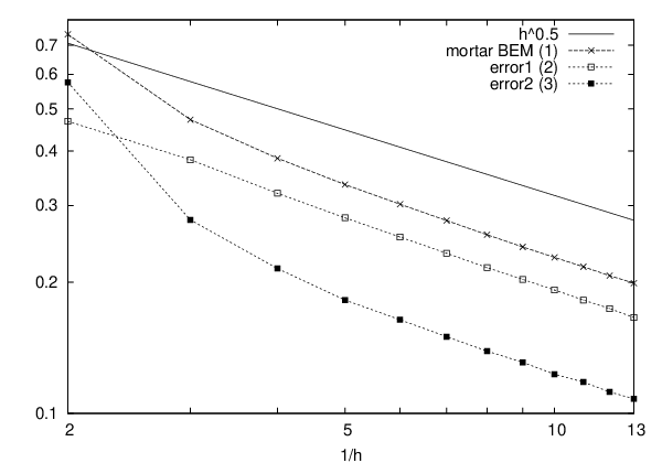
In the figures below we show different error curves, indicated by numbers () as follows.
| (1) | “mortar BEM” | |
| (2) | “error1” | |
| (3) | “error2” | |
| (4) | “conforming BEM” |
Here, denotes a conforming boundary element solution. Additionally, all curves are normalized by .
Therefore, to resume, an error curve (1) represents the upper bound (4.3) for the (normalized) error of the mortar BEM. Curves (2) and (3) are the two components of (1). Here, (3) controls the non-conformity of the mortar approximant . Curve (4) represents the error of the conforming BEM. In this case it is equivalent to the error in energy norm .
All results are plotted on double logarithmic scales versus . For our numerical experiments we always use rectangular meshes and in this section, refers to the length of the longest edge on , and as before.
Conforming sub-domain decomposition.
Experiment 1 (conforming mesh, results in Figure 4.1). First let us consider a conforming decomposition of into four sub-domains as indicated in Figure 2.1(a). Moreover, let us first test the case where the separate meshes on the sub-domains form globally conforming meshes (we take uniform meshes consisting of squares). The corresponding results are shown in Figure 4.1. Along with the curves (1), (2), (4) we plot the values of . The numerical results indicate a convergence of the order , for the conforming as well as the mortar BEM. According to the discussion above this is the best one can expect. The curves (1) and (2), referring to our upper bound (4.3) and the first term in (4.3), respectively, are almost identical. This means that the second term in (4.3), which in the next plots will be labeled by (3), is negligible in comparison. Indeed, in this symmetric case the jumps disappear and the numerical results vanish at the order of single precision. Therefore, in this plot, we do not show the curve (3).
We do not observe a logarithmical perturbation of the convergence in this range of number of unknowns. This may be caused by the fact that we are not including the -parts in the error since our results are, up to constant factors, upper bounds only for the semi-norm . Also, we do not know whether our bounds including the logarithmic terms are sharp.

Experiment 2 (non-conforming mesh, results in Figure 4.2). Now let us test globally non-conforming meshes. Again we use uniform meshes consisting of squares on each sub-domain. We mesh as in Figure 2.1(a) starting with 2, 3, 4, and 5 “slides” on , , , and , respectively and increase the number of slides in each sub-domain by one in each step of our sequence of meshes. The corresponding results are shown in Figure 4.2. Again, a convergence of the expected order is confirmed. Curve (3) indicates very fast convergence of the jumps . In the experiments below, however, we observe a slower convergence. In this particular sequence of meshes, where we increase the slides on the sub-domains by the same amount, the trace meshes from different sides on a particular interface edge approach each other in a certain sense. We conjecture that this specific situation (“approaching” conforming meshes) causes the fast convergence of the jumps.
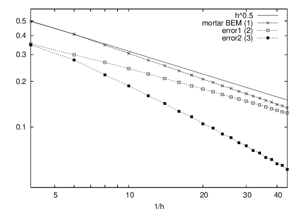
Experiment 3 (non-conforming mesh, results in Figure 4.3). For the next experiment we start with a mesh of four squares on each sub-domain (the sub-domains are again as in Figure 2.1(a)), and increase the numbers of slides on different sub-domains by different steps (increase by , , , slides on , , , , respectively). In this case both error parts, curves (2) and (3), behave like , confirming our a priori error estimate and thus the good performance of the mortar BEM. Let us note, however, that the part of the error expression (4.3) is an overestimation. Indeed, our substitution (4.3) for is not precise. On the one hand we replaced the term in (4.2) by (and the generic constant in (4.1) by ). On the other hand the term is of higher order than . According to (3.18) and by standard approximation theory there holds for any
This shows that is of higher order than . Note that, by the proof of Theorem 3.2 and since , one has the regularity Therefore, by (4.2) the term
is asymptotically equal to
and this dominates the error.
Non-conforming sub-domain decomposition.
Experiment 4 (non-conforming mesh, results in Figure 4.5). Finally, we consider the fully non-conforming mortar method, i.e. with non-conforming sub-domain decomposition and non-conforming meshes. We decompose into three sub-domains as in Figure 4.4 and use the initial mesh given there on the left. Then slides on sub-domains are increased in each direction by 3, 2, 1 on , , , respectively, in each step. The second mesh is on the right in Figure 4.4. Note that in each second step the cross-point between the sub-domains is a hanging node and our theory includes this case. The numerical results are shown in Figure 4.5 and again confirm the expected convergence of the mortar BEM.
In this case, the meshes for the Lagrangian multiplier are coarsenings of the trace meshes from on and , and of the trace mesh from on . We always join two elements of the respective trace mesh to form an element of the Lagrangian multiplier mesh, except for an odd number of elements of the trace mesh when one set of three elements is joined. The corresponding numbers of unknowns for the steps are listed in Table 1.

| dim() | dim() | |||
|---|---|---|---|---|
| 0.5000 | 0.1250 | 0.1667 | 27 | 4 |
| 0.3333 | 0.0625 | 0.0833 | 80 | 7 |
| 0.2500 | 0.0417 | 0.0556 | 161 | 11 |
| 0.2000 | 0.0313 | 0.0417 | 270 | 14 |
| 0.1667 | 0.0250 | 0.0333 | 407 | 18 |
| 0.1429 | 0.0208 | 0.0278 | 572 | 21 |
| 0.1250 | 0.0179 | 0.0238 | 765 | 25 |
| 0.1111 | 0.0156 | 0.0208 | 986 | 28 |
| 0.1000 | 0.0139 | 0.0185 | 1235 | 32 |
| 0.0909 | 0.0125 | 0.0167 | 1512 | 35 |
| 0.0833 | 0.0114 | 0.0152 | 1817 | 39 |
| 0.0769 | 0.0104 | 0.0139 | 2150 | 42 |
References
- [1] F. Ben Belgacem, The mortar finite element method with Lagrange multiplier, Numer. Math., 84 (1999), pp. 173–197.
- [2] F. Ben Belgacem and Y. Maday, The mortar element method for three dimensional finite elements, M2AN Math. Model. Numer. Anal., 31 (1997), pp. 289–302.
- [3] C. Bernardi, Y. Maday, and A. T. Patera, Domain decomposition by the mortar element method, in Asymptotic and Numerical Methods for PDEs with Critical Parameters, H. G. Kaper and M. Garbey, eds., 1993, pp. 269–286.
- [4] , A new nonconforming approach to domain decomposition: the mortar element method, in Nonlinear Partial Differential Equations and their Applications, H. Brezis and J.-L. Lions, eds., Pitman, New York, 1994, pp. 13–51.
- [5] A. Bespalov and N. Heuer, The -version of the boundary element method with quasi-uniform meshes in three dimensions, ESAIM Math. Model. Numer. Anal., 42 (2008), pp. 821–849.
- [6] D. Braess, Finite Elements: Theory, Fast Solvers, and Applications in Solid Mechanics, Cambridge University Press, Cambridge, 1997.
- [7] D. Braess, W. Dahmen, and C. Wieners, A multigrid algorithm for the mortar finite element method, SIAM J. Numer. Anal., 37 (1999), pp. 48–69.
- [8] A. Buffa, M. Costabel, and D. Sheen, On traces for H(curl, ) in Lipschitz domains, J. Math. Anal. Appl., 276 (2002), pp. 845–867.
- [9] A. Chernov, M. Maischak, and E. P. Stephan, -mortar boundary element method for two-body contact problems with friction, Math. Methods Appl. Sci., 31 (2008), pp. 2029–2054.
- [10] M. Costabel, Boundary integral operators on Lipschitz domains: Elementary results, SIAM J. Math. Anal., 19 (1988), pp. 613–626.
- [11] M. R. Dorr, The approximation theory for the -version of the finite element method, SIAM J. Numer. Anal., 21 (1984), pp. 1180–1207.
- [12] V. J. Ervin, N. Heuer, and E. P. Stephan, On the - version of the boundary element method for Symm’s integral equation on polygons, Comput. Methods Appl. Mech. Engrg., 110 (1993), pp. 25–38.
- [13] G. N. Gatica, M. Healey, and N. Heuer, The boundary element method with Lagrangian multipliers, Numer. Methods Partial Differential Eq. DOI 10.1002/num.20401.
- [14] P. Grisvard, Elliptic Problems in Nonsmooth Domains, Pitman Publishing Inc., Boston, 1985.
- [15] N. Heuer, Additive Schwarz method for the -version of the boundary element method for the single layer potential operator on a plane screen, Numer. Math., 88 (2001), pp. 485–511.
- [16] N. Heuer and F.-J. Sayas, Crouzeix–Raviart boundary elements, Report 07/5, BICOM, Brunel University, UK, 2007. Numer. Math., in press.
- [17] G. C. Hsiao and W. L. Wendland, A finite element method for some integral equations of the first kind, J. Math. Anal. Appl., 58 (1977), pp. 449–481.
- [18] J.-L. Lions and E. Magenes, Non-Homogeneous Boundary Value Problems and Applications I, Springer-Verlag, New York, 1972.
- [19] A.-W. Maue, Zur Formulierung eines allgemeinen Beugungsproblems durch eine Integralgleichung, Zeitschrift für Physik, 126 (1949), pp. 601–618.
- [20] J.-C. Nédélec, Integral equations with nonintegrable kernels, Integral Equations Operator Theory, 5 (1982), pp. 562–572.
- [21] J.-C. Nédélec and J. Planchard, Une méthode variationnelle d’éléments finis pour la résolution numérique d’un problème extérieur dans , RAIRO, 7 (1973), pp. 105–129.
- [22] E. P. Stephan, A boundary integral equation method for three-dimensional crack problems in elasticity, Math. Methods Appl. Sci., 8 (1986), pp. 236–257.
- [23] , Boundary integral equations for screen problems in , Integral Equations Operator Theory, 10 (1987), pp. 257–263.
- [24] T. von Petersdorff and E. P. Stephan, Decompositions in edge and corner singularities for the solution of the Dirichlet problem of the Laplacian in a polyhedron, Math. Nachr., 149 (1990), pp. 71–104.