UT-09-02
LTH 820
IPMU09-0014
Codimension-3 Singularities and Yukawa Couplings in F-theory
Hirotaka Hayashi1, Teruhiko Kawano1, Radu Tatar2 and Taizan Watari3
1Department of Physics, University of Tokyo, Tokyo 113-0033, Japan
2Division of Theoretical Physics, Department of Mathematical
Sciences, The University of Liverpool, Liverpool, L69 3BX, England,
U.K.
3Institute for the Physics and Mathematics of the Universe, University of Tokyo, Kashiwano-ha 5-1-5, 277-8592, Japan
F-theory is one of the frameworks where all the Yukawa couplings of grand unified theories are generated and their computation is possible. The Yukawa couplings of charged matter multiplets are supposed to be generated around codimension-3 singularity points of a base complex 3-fold, and that has been confirmed for the simplest type of codimension-3 singularities in recent studies. However, the geometry of F-theory compactifications is much more complicated. For a generic F-theory compactification, such issues as flux configuration around the codimension-3 singularities, field-theory formulation of the local geometry and behavior of zero-mode wavefunctions have virtually never been addressed before. We address all these issues in this article, and further discuss nature of Yukawa couplings generated at such singularities. In order to calculate the Yukawa couplings of low-energy effective theory, however, the local descriptions of wavefunctions on complex surfaces and a global characterization of zero-modes over a complex curve have to be combined together. We found the relation between them by re-examining how chiral charged matters are characterized in F-theory compactification. An intrinsic definition of spectral surfaces in F-theory turns out to be the key concept. As a biproduct, we found a new way to understand the Heterotic–F theory duality, which improves the precision of existing duality map associated with codimension-3 singularities.
1 Introduction and Summary
The Standard Model of particle physics with neutrino masses contains 20–22 flavor parameters, depending on whether the neutrino mass is Dirac or Majorana. The Yukawa couplings are the coefficients of scalar–fermion–fermion couplings in low-energy effective Lagrangian, and they can take arbitrary values. This is in sharp contrast to the interactions involving gauge bosons, where gauge symmetry controls everything and very few free parameters are left. The effective-field-theory model building succeeded in translating observed patterns of flavor parameters into the language of flavor symmetries and their breaking patterns, but it is hard to understand where the flavor symmetries come from.
In a wide class of string theory compactifications, however, quarks, leptons and Higgs boson arise from components of super higher dimensional Yang–Mills multiplets and Yukawa couplings descend from super Yang–Mills interactions. This fact provides hope to get more theoretical control over flavor structure of quarks and leptons. Even though string theory might eventually provide only a translation of known flavor structure in language of geometry, yet string theory compactifications with flavor structure under control would serve as a reliable framework in discussing issues as gravity mediated supersymmetry breaking, where both Planck suppressed interactions and flavor violating interactions should be brought under control.
The SU(5) model of grand unification with low-energy supersymmetry is perfectly consistent with the measured value of gauge coupling constants, and major aspects of flavor structure are understood in terms of approximate Abelian flavor symmetries (also known as Froggatt–Nielsen mechanism) consistent with Georgi–Glashow SU(5) unification. Yukawa couplings of up-type and down-type quarks are written as
| (1) |
in SU(5) GUT’s, where are indices and generation (flavor) indices. If all the matter fields—Higgs boson and matter fermions—arise from super Yang–Mills multiplet of higher dimensions with gauge group containing , and if all the Yukawa couplings originate from super Yang–Mills interactions of gauge group , then has to contain [1]. This means that the candidates for such framework are either one of Calabi–Yau 3-fold compactification of Heterotic string theory, M-theory compactification on -holonomy manifolds or Calabi–Yau 4-fold compactification of F-theory. Those three frameworks are mutually related by string duality, but not all the moduli space of the three frameworks completely overlap.
Moduli stabilization is well understood in F-theory Calabi--Yau 4-fold compactification.11 1 Reference [1] discusses structure of Yukawa matrices in -holonomy compactification of 11-dimensional supergravity with SU(5) unification. The Yukawa matrix of first term of (1) tends to have small values in diagonal entries relatively to off-diagonal entries. To our knowledge, this is not a phenomenologically successful pattern of Yukawa matrix. In order to avoid this problem in -holonomy compactification of M-theory, some of the assumptions in [1] have to be relaxed. 4-form fluxes stabilize complex structure moduli (including moduli of 7-branes), which correspond in Calabi–Yau 3-fold compactification of Heterotic string theory to vector-bundle moduli as well as complex structure moduli. Thus, (F-term part of) Yukawa couplings can be discussed in F-theory with everything under control, nothing in a black box.
It is now known how to determine the matter spectrum of effective theory below the Kaluza–Klein scale in generic supersymmetric compactification of F-theory [2, 3, 4, 5, 6]. Charged matter chiral multiplets are identified with global holomorphic sections of certain line bundles on complex curves. Complex structure of elliptic fibered Calabi–Yau 4-fold determines the divisors of those line bundles. Thus, one can even determine wavefunctions of the zero-mode chiral multiplets along the complex curves for a given complex structure of a Calabi–Yau 4-fold, using rather standard techniques in algebraic geometry [6]. Flux compactification can be used to determine the complex structure of a Calabi–Yau 4-fold.
A technical problem still lies in a process of calculating Yukawa couplings using the wavefunctions of zero modes. There is no question that Yukawa couplings are generated; massless charged matter multiplets in F-theory are identified with M2-branes wrapped on vanishing 2-cycles, and algebra of those 2-cycles determines what kind of Yukawa interactions are generated [1]. The question is how to calculate them. Yukawa couplings among charged matter multiplets are now believed to be attributed to codimension-3 singularity points in a base 3-fold [5, 4, 6]. Unlike Type IIB string theory, however, F-theory (or M-theory) lacks microscopic descriptions that are valid to any short distance scale, and an idea is necessary in how to deal with physics localized at/around the codimension-3 singularity points.
The references [4, 5] proposed a field theory formulation of super Yang–Mills sector associated with intersecting 7-branes, which we find is useful particularly for this purpose. Instead of developing microscopic quantum theory of F-theory, field theory on 8-dimensional spacetime is used, and unknown microscopic effects can be dealt with as higher order operators in (or ) expansion with unknown coefficients. Such a framework should be sufficient at least in determining certain terms in low-energy effective theory below the Kaluza–Klein scale at a controlled level of precision.
In this article, we construct gauge-theory local models22 2 We mean by a “local model” a theoretical tool to analyze physics associated with a local geometry of a Calabi–Yau. We do not use the word “model” in the way it is used in the Standard “Model”, Georgi–Glashow “model”, gauge mediation “models” etc. See section 2 for more explanations on what we mean by “local models”, as well as what one can do with them. of various types of codimension-3 singularities of F-theory compactification, and analyze the behavior of zero-mode wavefunctions around the codimension-3 singularity. Although the field theory framework of [4, 5] is used for this analysis, we found that one has to introduce branch cuts into the field theory and fields have to be twisted by Weyl reflection at the branch cuts, in order to deal with F-theory compactification on a Calabi--Yau with fully generic complex structure. This observation has never been made in the recent articles on F-theory, and hence the analysis of such local models has never been done before.33 3 Analysis of [5, 7] on codimension-3 singularities covers only non-generic choice of complex structure.
It has been known that the zero-mode wavefunctions decay in a Gaussian profile off the matter curves [8]. Here, is a normal coordinate to the matter curve. This result however, was obtained only for generic points on matter curves. Around codimension-3 singularity points on matter curves, we found that this statement is not always true. Depending upon the types of codimension-3 singularity and representations of zero-modes, the wavefunctions decay off the matter curves either in the Gaussian profile or in a slightly moderate form . All these results are obtained in sections 3 and 4; the latter section deals with codimension-3 singularities that appear in GUT model building.
The field-theory local models, however, can be used only to study behavior of zero-mode wavefunctions, and interactions of the zero modes only in a small region in a complex surface. Matter zero-modes of effective theory in 4-dimensions, on the other hand, are identified with global holomorphic sections of line bundles on complex curves. Without looking at this global issue, we do not even know how many matter multiplets are in the low-energy spectrum. We thus need both descriptions, and hence need to figure out how these two different descriptions of chiral matter are related. This is one of the goals of section 5. In other words, this is to clarify the relation between [4, 5] and [6].
Section 5 also provides a number of observations that are also interesting purely from theoretical perspectives. We found that the field expectation values satisfying supersymmetry conditions of the field theory formulation [4, 5] define objects that are called canonical-bundle valued Higgs bundles in Mathematical literature. A spectral cover is defined for a canonical bundle valued Higgs bundle, which is a divisor of a total space of a canonical bundle. Although discriminant locus of elliptic fibered Calabi–Yau manifold in F-theory corresponds to a 7-brane, and is usually regarded as generalization of D7-branes in Type IIB string theory, yet we find that the spectral cover is more natural generalization of the notion of a system of intersecting D7-branes. The notion of Higgs bundle and its spectral cover allows us i) to naturally extend the characterization of chiral matter multiplets in the Type IIB string theory [9, 10] into F-theory,44 4 Although charged matter multiplets in a given representation have their own matter curve, there is not always an irreducible piece of the discriminant locus specifically for the representation. This subtlety becomes clear only when geometry around codimension-3 singularity is studied carefully. and ii) to provide a totally new way to understand the duality between the Heterotic string theory and F-theory, and a new way to determine the duality map.
With this better understanding in the Heterotic–F theory duality, we can study what is really going on in F-theory in geometry around codimension-3 singularity points (section 5.3). The duality tells that ramification of spectral cover and 3-form potential field (in M-theory language) are the only ingredients to think about. Twist of a line bundle on a spectral surface has long been predicted in Mathematical literature, and there is nothing unexpected from ramification. We found that 3-form field background is single valued, even when 2-cycles are twisted around a point of codimension-3 singularity.
In section 6, we return to physics application. Using the field theory formulation of [4, 5] and the zero-mode wavefunctions of the local model in section 4, we find that the up-type Yukawa matrix of Georgi–Glashow SU(5) models generated from a codimension-3 singularity with enhanced singularity is rank-1 at the leading order for generic choice of complex structure of Calabi–Yau 4-fold. This solves the problem raised by [7]. We also argue that the overlap of Gaussian tails of zero-mode wavefunctions may have significant contributions to the Yukawa eigenvalues of lighter generations, a possibility that was not pointed out in [11].
An incomplete list of other articles that discussed physics of F-theory in the last several months includes [13, 14, 15, 16, 17, 18, 19, 20, 21, 22, 23, 24] and other articles cited elsewhere in this article.
Reading Guide: Local behavior of zero-mode wavefunctions are studied in sections 3 and 4, and are used in the discussion of Yukawa couplings in section 6. Section 5 provides theoretical foundation to an idea that bridges a small gap between sections 3–4 and section 6, but the idea itself may look reasonable on its own. Thus, section 5 can be skipped for those who are interested in Yukawa couplings and think that the idea is acceptable.
Section 5, on the other hand, deals with theoretical aspects of F-theory, and sheds a new light on Heterotic–F theory duality. Sections 3 and 4 provide “experimental data” to the theory in section 5, but we prepared this article so that section 5 can be read separately from the other parts of this paper. It is an option for those not interested in Yukawa couplings so much to read only section 5.
This section is meant also to serve as a brief summary of this article.
2 Field-Theory Local Model of F-theory Geometry
An effective theory with supersymmetry is obtained when F-theory is compactified on an elliptic fibered Calabi–Yau 4-fold
| (2) |
We assume that is given by a Weierstrass equation
| (3) |
and and are global holomorphic sections of and , respectively. The discriminant of this elliptic fibration is given by
| (4) |
which is a complex codimension-1 subvariety (divisor) of .
The discriminant locus may have several irreducible components,
| (5) |
where are divisors of , and their multiplicities. Calabi–Yau 4-fold develops singularity along the discriminant loci with multiplicity . When has singularity along an irreducible component , then its multiplicity is . The multiplicity is for singularity, and for () [25, 26] (and references therein).
When a complex structure moduli of is chosen allowing such a locus of -- singularity in , its low-energy effective theory has a gauge field with the corresponding gauge group. Such a compactification becomes a candidate for the description of supersymmetric unified theories, supersymmetric Standard Model or hidden sector triggering dynamical supersymmetry breaking. When the discriminant locus is written as
| (6) |
then matter multiplets charged under the gauge group on arise at the intersection .
Some aspects of low-energy effective theory do depend on the full geometry of . One example is the Planck scale (Newton constant) of the 3+1-dimensional Minkowski space. Many aspects of gauge theory associated with the discriminant locus , however, depend only on the geometry of around . In order to study the profile of wavefunctions of zero-mode matter multiplets, one needs to study only the geometry along the codimension-2 loci of . There have also been indications that Yukawa couplings essentially originate from codimension-3 loci of . Thus, one can go a long way in phenomenology by studying only the local geometry of F-theory compactification.
References [4, 5] formulated a field theory on “” that can be used to derive low-energy effective theory of zero modes along (including those along ). Field contents on are summarized in Table 1.
| vector | chiral | multiplet | anti-chiral | multiplet | |
|---|---|---|---|---|---|
| Bosonic fields | |||||
| Fermionic fields |
The field on corresponds to transverse fluctuation of D7-branes in Type IIB orientifold compactification on a Calabi–Yau 3-fold . If is a Type IIB Calabi–Yau orientifold of , has a global holomorphic 3-form , where now a set of local coordinates () is chosen on . The field in Type IIB Calabi–Yau orientifold corresponds to in formulation of [4, 5] through . Since the base 3-fold is not necessarily a quotient of a Calabi–Yau 3-fold in general F-theory compactification, the global holomorphic 3-form does not necessarily exist. References [4, 5] found that using instead of is the right way to formulate the field theory.
Suppose that a zero mode exists in for a given compactification; that is, . Non-vanishing vacuum expectation value (vev) in corresponds to deforming geometry of , so that the irreducible decomposition of discriminant in (6) becomes
| (7) |
with and and are topologically the same as in . Singularity along the irreducible discriminant locus is reduced from55 5 Here, we abuse language and do not make a distinction between Lie algebra of -- type and singularity type of the corresponding one of --. to the commutant of in . Suppose that takes its value in . Then, the irreducible decomposition of is of the form
| (8) |
The hypermultiplets in the representation of unbroken symmetry are localized along a complex curve . Chiral (and anti-chiral) matter multiplets exist in low-energy effective theory of 4-dimensions, if there are zero modes on the curve . Because the localization of these matter fields are solely due to the vev of , one can use the field theory on with non-vanishing to study behavior of localization of the -charged matter on the curve and behavior of zero modes along the curve.66 6 Note that the field theory is formulated on a complex surface , which is neither identified with the discriminant loci nor in the presence of . To borrow an intuitive picture of Type IIB string in Figure 1, any points with the same coordinates on 7-branes are identified with a point with on “”, and the difference in the coordinate is ignored; configuration of 7-branes in the direction are encoded as that depend on in the field-theory formulation.
Codimension-2 singularity loci in (6), however, are not always obtained as associated with a non-trivial globally defined on “”. Two cartoon pictures in Figure 1 describe how D7–D7 intersection arises in Type IIB string theory.
 |
 | |
| (a) | (b) |
Not all D7–D7 intersection curves are obtained by turning on a vev or defined globally on (i.e., by deforming D7-brane configuration continuously), but local geometry around D7–D7 intersection curves is essentially the same in (a) and (b) of Figure 1. Matter multiplets arise from open strings connecting two stacks of D7-branes, and are localized along the 7-brane intersection curve. They would not care about the global configuration of D7-branes, except that they interact at points where D7–D7 intersection curves meet one another. Thus, the localization of massless matter multiplets will not be affected by the global configuration of irreducible discriminant loci (i.e. 7-branes) in F-theory. An important idea of [5], which essentially dates back to [8], is that local geometry of F-theory compactification is approximately regarded as deformation of type singularity to type for appropriate choice of and , and a corresponding gauge theory can be used as an (approximate) local model of local geometry to study physics issues such as the localization of matter multiplets and their interactions.
Not all the aspects of low-energy effective theory in 4-dimensions depend on all the details of the elliptic fibered Calabi–Yau geometry , as we mentioned before. It is best to focus on relevant parts of geometry to determine various aspects of the effective theory. Newton constant depends on the whole volume of , whereas the gauge coupling of a non-Abelian gauge theory on depends only on . To study wavefunctions of localized zero-modes of charged matter, one needs to look at the entire compact matter curves (codimension-2 loci of ), but only a region around a codimension-3 singularity point in will be sufficient in studying individual contributions to Yukawa couplings. To study Yukawa couplings, local patches of and an appropriate Lie algebra can be chosen around codimension-3 singularity points, so that the local geometry is studied by a field theory local model with gauge group , which is broken down to by . Such field-theory local models around codimension-3 singularity points are glued together along the matter curves, in order to obtain low-energy effective theory below the Kaluza–Klein scale. We do not need an 8-dimensional field theory description that covers the entire discriminant locus . This is a radical yet powerful idea.
In sections 3 and 4, we will construct field theory local models for various types of codimension-3 singularity points in F-theory and study the behavior of zero-mode wavefunctions. Although there are so many different choices of topology of Calabi–Yau 4-fold and four-form flux on it, only a limited number of types of local geometry around codimension-3 singularity points. Thus, the local models are quite universal. Yukawa couplings generated in such local models are discussed in section 6, and we will discuss how to glue the results of these local models together to obtain low-energy effective theory in sections 5 and 6.77 7 Possible limitation of this approach of gluing local descriptions together is also discussed in section 6.2. See discussion that follows (236).
Reference [5] determined the (leading order part of the) Lagrangian of the field theory formulation on 8-dimensions, and this Lagrangian is used in studying the field theory local models. We quote the Lagrangian from [5] in the appendix A, after clarifying details of conventions and correcting typos in signs, phases and coefficients.
3 Generic Rank-2 Deformation of Singularity
In order to construct field theory local models for a local geometry, we need to determined field vev and corresponding to local geometry of a Calabi–Yau 4-fold and a local configuration of 3-form potential. We begin by mapping the complex structure of the Calabi–Yau 4-fold into the vev of the field in sections 3 and 4. The 4-form flux background is implemented in field theory in section 5. We only discuss local models until section 6, and hence complex surfaces “’’ on which field theory is defined is regarded as a non-compact space.88 8 As we already mentioned in the previous section, “” is not identified with a specific divisor in the base 3-fold .
The mapping between the Calabi–Yau geometry and the values of has been first used in [8]. The main idea is that the generic deformations of surface singularities of type —one of , or —are parametrized by , where is a Cartan subalgebra of Lie algebra , and its Weyl group. When we consider a local Calabi–Yau geometry that is a fibration (or family) of a deformation of a surface singularity of type over a base space , the local geometry is described by a gauge theory with gauge group . The variation of the deformation parameters of the fiber geometry over are encoded in varying over in the field-theory description. The dictionary between the defining equation of deformation of singularity of type and the parametrization of deformation by was well well-established in [27]. Thus, the dictionary can be used to translate the local geometry naively into , if one ignores the difference between and .
Most of the explicit studies in the literature essentially deal with deformation over a non-compact complex curve . The gauge group is often chosen to be just one-rank larger than the singularity (symmetry) that remains over . The consequence is simple: the hypermultiplet is localized at points where is enhanced to , with a Gaussian wavefunctions around the enhancement points [8]. But the idea itself is more general and we can apply it to for cases with a complex surface . It is a natural guess to choose of a local model to be two-rank larger than left unbroken over . This choice is proved to be correct for all the examples we study in this article. We will denote the base space as hereafter.
Calabi–Yau 4-fold geometry of F-theory compactification is much more general than the one coming from Calabi–Yau orientifold of Type IIB string compactification. In addition to the twist, and a twist that yields “non-split” singularity locus, there is another kind of twists generically in F-theory compactification, which corresponds to the difference between and mentioned above [28]. To our knowledge, not much discussion is found in the literature how to deal with this Weyl-group twist of F-theory in the field theory description. We will construct local models for geometry with this twist in section 3.2, by using 8-dimensional field theory with branch cuts, and explain an useful idea is studying such field theory.
To begin with, let us study most generic deformation of singularity in F-theory. Since we are interested in application to study of local geometry around codimension-3 singularities, we only consider 2-parameter deformation of singularity. The most generic form of deformation of surface singularity to is given by two parameters, and :
| (9) |
When and are set to zero, singularity is restored. An alternative parametrization of deformation is99 9 The deformation parameters are shifted from to , but this overall “center-of-mass” shift is irrelevant because it is absorbed by the shift of the origin of the coordinate .
| (10) |
in . The relation between and is
| (11) |
Both are invariant functions of Weyl group of , which is permutation of and .
When the deformation parameters and in (9) are promoted to functions of local coordinates of a non-compact base space , the equation (9) now defines a family (fibration) of surface singularity over deformed to . If a local geometry is given approximately by (9), then and are determined from (11). Local geometry given by (9) corresponds to a field-theory local model with non-vanishing vev1010 10 “” here is a constant associated with normalization of the field , and is largely unimportant in physics. See the appendix A for more details.
| (12) |
the field vev varies over the local coordinates of , if do. The gauge group of this field theory is , but only symmetry1111 11 See discussion below for whether gauge fields of Abelian factors remain massless in the low-energy effective theory. remains unbroken in effective theory, if and do not vanish at generic points of .
3.1 Three Intersecting D7-branes
We start with a choice for the values of as functions of which give rise to the well understood configuration of three intersecting D7-branes:
| (13) |
where are proportionality constants. The irreducible components of discriminant locus,1212 12 Although (9) does not define an elliptic fibration, it does contain a fibration of 1-cycle in plane, and the “discriminant locus” (14) is where the 1-cycle shrinks to zero size.
| (14) |
behaves as in Figure 2 (a).
 |
 | |
| (a) | (b) |
Since the component of the discriminant locus (i.e., 7-brane) further factorizes into and , this is nothing more than an F-theory description of a well-understood configuration in Type IIB string theory; three stacks of D7-branes intersect at angles, and one of the three stacks consists of D7-branes. We begin with this almost trivial example, just to get started. The corresponding vev of is
| (15) |
which is obtained by solving (11) and substituting the explicit form of and in (13).
The irreducible decomposition of is1313 13 There is no reason within this local model that the massless components of the vector fields for the two U(1) factors are gone from the spectrum. Whether they remain in the massless spectrum of effective theory below the Kaluza–Klein scale, however, is a more global issue.
| (16) |
in this case, where the two signs on the shoulder indicate the charge under and respectively of a given irreducible component. Zero-mode equations,
| (17) | |||||
| (18) | |||||
| (19) |
follow1414 14 (17–19) are not precisely the equations of motions obtained from (249). is missing from (17), for example. True equations of motions are solved with separation of variables, but the equations for the wavefunctions of zero modes are obtained by simply dropping derivatives in the Minkowski directions from the equations of motions. from the action1515 15 By taking the coordinates for orthonormal metric locally and promoting to a covariant derivative and by , one finds that these set of equations of motions have R-symmetry of 16-SUSY Yang–Mills theories; (20) (21) where and are left-handed spinors, just like . This serves as a check of various coefficients appearing in the Lagrangian (249). (249). These equations should be solved separately for each irreducible component, , and their hermitian conjugates, in the presence of a common background such as (15). As long as the background preserves supersymmetry, the zero mode wavefunctions of and should be the same as those of and .
The zero mode equations can be written down more explicitly, if we assume that we can take1616 16 Although metric of should exhibit certain form of singularity along discriminant loci such as in (6) (e.g., [29]), one should note that the “” here is a base space and is not a divisor of . It is not clear what kind of metric should be used here. We just adopt the simplest possibility here, which may be to ignore gravitational backreaction and consider only the Yang–Mills sector. a local coordinate system of so that the metric is locally approximately orthonormal, .
| (22) | |||
| (23) | |||
| (24) | |||
| (25) |
where and . () corresponds to charges of a given irreducible component under the background ; and are read out from or . We set , because we are interested in zero-modes that become chiral multiplets of supersymmetry in 4-dimensions.
The partial derivatives () are covariant derivatives involving a gauge field that corresponds to four-form flux on a Calabi–Yau 4-fold. Before sections 5 and 6, we assume that this gauge field background has negligible effects in determining zero-mode wavefunctions in a local region near points of codimension-3 singularity. Once they are ignored, then one can see that the zero mode equations for in the component are the same as those of in the component . Chirality, the difference between the number of zero modes in - representation and representation, comes purely from the gauge field. But, obtaining chiral spectrum at low-energy and generating Yukawa interactions among them are completely separate issues. The topological aspects of gauge field on the entire compact discriminant locus is essential for the former, whereas only local geometry on is presumably relevant to the latter. As long as we discuss the Yukawa interactions, we ignore the gauge field background for now.
It is not difficult to find a zero-mode wave function under the background (15). Since [resp. ] does not depend on [resp. ], one can seek for a wavefunction that does not depend on [resp. ] for the irreducible components and [resp. and ]. For the and components,1717 17 We assume that and are chosen real and positive, which is always possible without a loss of generality; one can redefine the phases of the coordinates and , if and are not real and positive.
| (26) |
One can also see from the zero-mode equations that the coefficient can be holomorphic functions of , yet the solutions above satisfy all the equations; no dependence is allowed, however, because of in (23, 25). Thus, this zero mode is Gaussian in the direction, and is localized on a complex curve given by . Along the curve parametrized by , the zero mode should be a holomorphic function of , which is not required to have any particular structure (such as pole or zero) at the codimension-3 singularity point . In Type IIB language, these zero modes correspond to open strings connecting D7-branes and -th D7-brane. Although another (-th) D7-brane also passes through the point ,the open strings in and are not affected by the presence of the -th D7-brane, quite a reasonable conclusion.
Similarly, for the component,
| (27) |
This is Gaussian in direction, and is localized along the curve . The coefficient function can now be a holomorphic function of , and the wavefunction in this local region is determined, once the behavior of is determined. The holomorphic function is not required to have any particular structure at ; this is an F-theory description. In type IIB interpretation, these zero modes correspond to open strings connecting D7-branes and -th D7-brane.
3.2 Generic Deformation of to
The first case (13) was a suitable choice in order to get three stacks of intersecting D7-branes in type IIB picture. However, that choice may not be the most generic deformation of singularity down to , because the zero locus of in (13) has a double point where also vanishes. Not all the deformations of should be like that. Instead, one can think of the following form of deformation:
| (28) |
where local coordinates are chosen so that the expressions above become simple. The essence of this case is that there is a common zero of and on , and no further assumptions are made.
The second case of the deformation of singularity is described by a field theory local model with given by1818 18 It is not absolutely obvious whether the vev can be diagonalized at . The -matrix valued may become a rank-2 Jordan block with a degenerate eigenvalue . We will be naive about anything around the branch locus () in the rest of this section, and similarly in section 4. We will return to this issue in section 5, however, and develop an argument that gets around this issue.
| (29) |
This follows from solving (11) and substituting (28). In this case, an irreducible decomposition1919 19 The vector field for the part does not remain massless in the effective theory below the Kaluza–Klein scale; we know this only from this local model. The vector field for the U(1) factor, however, may or may not remain massless, depending on more global aspects of compactification.
| (30) |
is more appropriate, because and turn into one another in the monodromy around . The two components and that form a doublet solution turn into one another, when they are traced along a path going around the branch locus .
Here, we start with a gauge theory whose gauge group at each point isi , because (9) defines a deformed surface singularity for each point in . independent vanishing 2-cycles are buried at , and there are two other independent topological cycles that we define now. For a given point , let the two roots of
| (31) |
be and . Then, the two independent non-vanishing cycles can be chosen as
| (32) | |||||
| (33) |
As varies over complex surface , the value of changes and turns into and vice versa around the branch locus . The fields and are associated with membranes wrapped on and , respectively, and this is why becomes and vice versa in a monodromy around the branch cut. At the same time, the -Cartan part of the vev of ,
| (34) |
becomes of its own around the branch locus . Overall, we need to introduce a branch cut extending out from the branch locus , and the -adj. fields are glued to themselves after twisting by transformation—Weyl group of algebra—across the branch cut. This is not a simple theory of fields in the -adj. representation. Since the branch locus passes right through the codimension-3 singularity point , we cannot take a local description for this codimension-3 singularity point that is free of this branch locus and twist.
Such a field theory description with branch cut and twist along the branch cut is quite common in generic configuration of F-theory compactification. The non-split singularity locus corresponding to -adj gauge theory with a twist by outer automorphism of algebra is considered in [28]. Reference [28] also discusses the twist by an element of Weyl group. The necessity of the twist by the Weyl group above is traced back to the fact that the deformation of singularity of type is parametrized by , not by . In order to obtain an effective theory with an unbroken gauge symmetry, one only has to maintain a family of undeformed untwisted (that is, split) surface singularity over . The deformation parameters (varying over ) are in , where and are the Cartan subalgebra and Weyl group of whose commutant in becomes . Generically, we should expect twists by in field theory local descriptions in F-theory compactification.2020 20 Charged matters are localized in codimension-1 loci of , because that is where one of eigenvalues of vanishes. The branch loci is where two eigenvalues of become degenerate, and they are also codimension-1 loci in . In F-theory compactification down to 5+1 dimensions, is a complex curve, and generically the matter loci and branch loci are isolated points on , and one can take a local region around a matter locus, so that branch loci are not contained in it. In compactification down to 3+1 dimensions, however, is a complex surface, and codimension-1 matter curves and branch curves generically intersect. This is why the branch locus and Weyl-reflection twists are inevitable in the field-theory description for compactifications down to 4-dimensions.
Aside from the branch locus where more than one eigenvalues are the same, and act separately on each of the two weights of doublets. Thus, we still have a zero-mode equations (22–25) separately for and . Although it is not easy to find an exact solution of these zero-mode equations for general form of , there is a common structure that any solutions of (22–25) satisfy. To see this, let us note first that are given locally by
| (35) |
for some function , because of (23). Equations (24, 25) now imply that
| (36) |
for some (locally) holomorphic function . Now (22) is the only constraint we still have:
| (37) |
For example, when ,
| (38) |
and the Gaussian solution in (26) corresponds to the one with sign here.
One can see that is positive definite, does not have a zero mode, and hence its inverse exists. Thus,
| (39) | |||||
| (40) |
are also obtained from . Thus, for any holomorphic functions , a solution exists for the zero-mode equation. However, the zero-mode solutions are not in one-to-one correspondence with the local holomorphic functions . vanishes wherever is holomorphic, and hence the behavior of at is irrelevant to the zero-mode wavefunctions. Therefore, depends only on on the locus, and so do , because they are related to through (24, 25). Since locus is the matter curve, zero-mode solutions are in one-to-one correspondence with local holomorphic functions (sections of a line bundle in general) on the matter curve.
Monodromy around the branch locus , or equivalently the gluing after -twist, can be implemented in this set of partial differential equations. The following description leads to a key observation later on in this article. An idea is to replace the local coordinate system from to
| (41) |
This is not a one-to-one map.
| (42) |
because and are mapped to the same point in . Let us introduce a new surface , where local coordinates are . A loop around the branch locus in is lifted to a path from to in . The new space is a 2-fold covering space of . Now, we define at as , at as . is , and becomes . The expressions (39, 40) are regarded as those on the covering space as well, with and now being single-valued functions on the covering space. We can also use as the local coordinates of this covering space. What really matters to the zero-mode wavefunctions is the residue of along the pole locus at , or equivalently modulo any functions generated by .
The covering surface is regarded as a space swept by all possible values of —eigenvalues of —for , because for a given point are resolved in . It is identified with a subspace in a space with coordinates , given by
| (43) |
This defining equation of is the same as that of the irreducible component of the discriminant locus, but they are different objects. The irreducible component of the discriminant is a divisor in . On the other hand, (and its eigenvalues) should transform as sections of canonical bundle of , , and hence the space with coordinates is the total space of , denoted by . Thus, the covering surface is regarded as a divisor of . In the generic deformation of singularity to ,
| (44) |
is a degree-2 cover of . is the ramification locus in , which corresponds to the branch locus in . The matter curve is on , which is mapped to curve in . See Figure 3. The function on the covering space transforms as . Thus, is not just a function on the covering space , but it is a section of a bundle containing2121 21 Since we have ignored gauge field background in this section, we cannot determine the other factor in the bundle associated with the gauge field background here. We will come back to this issue in section 5. a factor .

Let us now return to a particular case with the doublet background (29), before closing this section. Although we have not succeeded in solving this set of partial differential equations analytically, it is still possible to discuss the asymptotic behavior of the zero-mode solution.
In the large limit, and
| (45) |
is large even along the matter curve, where is small, but remains small. The zero-mode wavefunction will have larger value in the component, and it may decay as in Gaussian profile, , because is linear in the normal coordinate of the matter curve, .
This Gaussian profile of zero modes across the matter curve will no longer be a good approximation near the codimension-3 singularity point ; the first term of the expansion of above simply does not give a good approximation to . We can still study behavior of the zero mode wavefunction in a region with large and sufficiently small . All the details are found in the appendix B. Quoting (271) here,
| (46) |
This solution is still localized along the matter curve, because it decays as for large . This wavefunction does not fall off as quickly as Gaussian . Such a profile of wavefunction has never been discussed in the literature, and this is interesting on its own.2222 22 Only the leading order (linear) terms were kept in (28), and one should be aware that this profile follows only in a region where (28) is a good approximation. It should also be noted that both and components have equally large value in this region, although only is large and is small in the large and small region.
The zero-mode wavefunction in this doublet background (29) has small components in this region, but components are comparable to . We have2323 23 Here, we talk about the zero mode wavefunction in the representation of the background (29), and hence that of irreducible component. The zero mode wavefunction of the component is obtained by multiplying to the components.
| (47) |
This two-component (0,1)-form on can be expressed as a single component (0,1)-form on . In the region with large and small , , and
| (48) |
The monodromy around the branch locus in the zero-mode wavefunction can be traced by looking at ; becomes and vice versa in this process, just as we anticipated before. The same process corresponds to going from to in the (0,1) form solution on the covering space .
4 Generic Deformation of Singularity for GUT Models
We have studied the field theory local model of generic deformation of singularity down to . Such a generic configuration around a point of codimension-3 singularity in F-theory is much more complicated than just having intersecting D7-branes, but we now know how to deal with them.
One of the most important advantages of using F-theory as opposed to Type IIB string theory is that all the Yukawa couplings can be generated even in SU(5) GUT gauge group. The same technique can be applied to F-theory compactification used for GUT model building, and this is the subject in this section.
In order to preserve an unbroken SU(5) gauge symmetry, an elliptic fibered compact manifold should be given by an equation of the form [28]2424 24 When the elliptic fibration is given by an equation where are sections of certain line bundles on , we need for , in order to have a locus of split singularity at [28]; here denotes local coordinates on collectively, and the coordinate of normal to . Local functions here correspond to in (49), and and can be regarded as higher-order terms in the expansion in . There is no rationale to maintain only and and drop all other higher order terms purely in the context of F-theory, although it will be clear how to modify the rest of this article when such higher order terms are included in (49). Here, we adopted the form (49), because the duality map between F-theory and Heterotic string theory [30, 31, 4, 6] is to identify precisely with in (192), and in (49) with those in (191). We will discuss Heterotic–F theory duality in section 5.
| (49) | |||||
where are coordinates for the elliptic fiber of the elliptic fibration in (3), and is the coordinate normal to the discriminant locus of the GUT gauge group. are functions2525 25 They are sections of appropriate line bundles on , but we do not pay much attention to global issues here. of local coordinates of . Terms higher order in are omitted from this equation. Local geometry with singularity for SO(10) GUT models can be obtained by simply setting . For the purpose of studying geometry for SU(5) or SO(10) GUT models, therefore, it is very convenient to start from the defining equation (49).
4.1 Codimension-3 Singularities in GUT Models
Let us begin with SU(5) GUT models. For this purpose, we do not need to make further assumptions on the sections . The discriminant of this elliptic fibration is given by
| (50) | |||||
is the locus of GUT gauge fields (codimension-1 singularity in a base 3-fold), and there are two matter curves (codimension-2 singularities) specified by and . is where matter multiplets in the - representations are localized, while matter in the - representations are at the curve , with
| (51) |
The curve is where the singularity in -surface is enhanced from to , while the enhanced singularity is along the curve . The discriminant becomes (as in singularity) when , whereas for (as in singularity).
There are some isolated codimension-3 singularities along the matter curves.

On the curve, they are at [32, 6]2626 26 In traditional literatures on F-theory like [28, 32], a section of a line bundle in such literature roughly corresponds to , to and to in F-theory compactification that preserves an singularity locus. See [6] for the precise relation between them. In the traditional notation, the type (a) singularity corresponds to the , and type (d) to the loci.
- •
type (a): common zero of and ,
- •
type (d): common zero of and .
This is where the coefficient of the term in the discriminant vanishes.
On the curve they are at:
- •
type (c1): common zero of and but [6], with
| (52) |
for a local defining equation (49). In what follows, we will see that the deformations of , and singularity, respectively, to are good approximation of local geometry of each of the three types of codimension-3 singularities above. Field theory local model with , and gauge groups, respectively, can be used to analyze physics localized at these types of codimension-3 singularities. All the three types of rank-2 deformation of –– singularity to appear in F-theory compactification for SU(5) GUT models. Using the local models, we will analyze the behavior of matter zero-mode wavefunctions around those codimension-3 singularities.
4.1.1 Type (a) Singularity:
Let us begin with the type (a) codimension-3 singularities. The type (a) codimension-3 singularity is where Yukawa couplings of the form
| (53) |
is believed to be generated. This type of interaction becomes up-type Yukawa couplings in Georgi–Glashow GUT’s, and down-type Yukawa couplings and mass terms of colored Higgs multiplets in flipped SU(5) GUT’s. Thus, this type of local geometry of F-theory compactification is of a particular phenomenological interest.
The coefficient functions in (49) corresponds to those of defining equations of spectral surface of a vector bundle in Heterotic compactification. Thus, and at the type (a) codimension-3 singularities means that the structure group of vector bundle is reduced to in Heterotic language, and the singularity is enhanced to , the commutant of in . Even without a knowledge of Heterotic–F theory duality, the criterion in [28] tell us that the singularity is enhanced to , because when and when . Therefore, it is an obvious guess to use gauge theory for the field theory local model of the type (a) codimension-3 singularities, although not all F-theory vacua have Heterotic dual.
The most generic deformation of singularity can be given by a local equation
| (54) |
When all of and are set to zero, this equation defines a complex surface in a space with singularity. The coordinates correspond to the direction of elliptic fiber, and to a direction normal to . The six deformation parameters and in (54) are functions of local coordinates () on . Since the rank of is six, the generically chosen will completely resolve the singularity.
Reference [27] shows that the most generic deformation of A-D-E singularity is parametrized by . In the case of deformation of singularity, we can choose six complex numbers () by choosing a basis in the Cartan subalgebra of . The deformation parameters in (54) are homogeneous functions of ’s of degree whose explicit forms are given in [27]. When we set the homogeneous degree of the three coordinates to be 4, 6 and 3, respectively, and the deformation parameters ’s as 1, the equation of singularity (and its deformation) is a homogeneous function of degree 12, the dual Coxeter number of . When a local geometry of F-theory is a family of surface with deformed singularity over a base space , i.e. a local equation of geometry is approximately (54) with some functions on , the field theory description of [8, 5] is to employ gauge theory with non-vanishing vev in the -valued complex scalar (or holomorphic 2-form) field given by corresponding ’s (so, actually the vev is in the Cartan subalgebra).
We are, however, interested in deformation of singularity to , and want to preserve SU(5) unbroken symmetry. Thus, the deformation of interest is parametrized by two complex numbers for a given point on . In the local equation of geometry (49), and correspond to the two deformation parameters. To see only the local geometry around a family of deformed surface singularity, we consider the following scaling:
| (55) |
and we zoom in to the singular locus as . The deformation parameters and should also scale to zero toward a point of type (a) codimension-3 singularity, in order to restore singularity in the fiber surface.
| (56) |
turns out to be the appropriate scaling, as we will see. All other coefficients in (49), namely , and , remain finite and do not scale as . All the terms involving , and scale as , , and , and become relatively small compared with all other terms scaling as . Thus, those terms are irrelevant to the geometry close to the codimension-3 singularity. We therefore drop those terms in the following argument.
After a change in the coordinates from to
| (57) |
the local defining equation (49) becomes
| (58) | |||||
Here, and . Irrelevant terms have been dropped. This equation is ready to be identified with (54).
In order to determine ’s and hence the vevs of in terms of and , we need a little more preparation. Not all six degrees of freedom of ’s are necessary, because the geometry (49) preserves symmetry. Some two dimensional subspace for unbroken symmetry has to be identified. To this end, we start off with a review of a (rather common) convention of choice of basis in describing the Cartan subalgebra of . Consider a 7-dimensional vector space spanned by a basis vectors , and introduce a bilinear form in this basis. A special element of this vector space is defined by . The orthogonal complement of , which is a 6-dimensional space, is identified with the dual space of the Cartan subalgebra of . Six independent vectors
| (59) |
can be chosen as the simple roots. The maximal root becomes , and the intersection form of and is described by the extended Dynkin diagram of .
The Cartan subalgebra of is a dual space of the six dimensional space given above. Using the bilinear form, however, the Cartan subalgebra can be identified with the same six-dimensional vector space. Thus, an arbitrary element in the Cartan subalgebra can be written as
| (60) |
where the coefficients satisfy . It is conventional (at least in [27]) that the independent six numbers () are chosen as
| (61) |
When the Cartan subalgebra is parametrized by , functions symmetric under any permutations of ’s are defined by
| (62) |
The permutation group of six elements is the Weyl group of generated by . Functions of ’s symmetric under the full Weyl group of ——are constructed from the -invariant functions ; explicit form of are found in [27]. The deformation parameters ’s in (54) are related to the Cartan parameters ’s in this way.
An subalgebra can be generated by simple roots and . Since
| (63) |
satisfies and , vev of can be introduced in this rank-1 subspace of the Cartan subalgebra of in order to deform the singularity so that singularity remains. This choice corresponds to
| (64) |
One can also see that
| (65) |
satisfies and . Roots and can also generate another subalgebra of . This choice corresponds to
| (66) |
Thus, when the vev of is in the direction parametrized by as above, then the singularity of is deformed and singularity remains.
An subalgebra of can be generated by . Thus,
| (67) |
satisfies , and the vev of should be introduced in this rank-1 subspace of the Cartan of , if singularity is to remain. This choice corresponds to2727 27 Weyl reflection in the direction of takes in (67) to , and to . and are the simple roots of , then.
| (68) |
The three generators (63, 65, 67) of the Cartan subalgebra of span a two dimensional subspace. Two generators (63) and (67) can be chosen as independent,
| (69) |
and (65) can be obtained as a linear combination of both with . All the roots are neutral under the two-dimensional subspace of the Cartan, and vev of in this subspace does not break the SU(5) symmetry (or deform the singularity) generated by . The -parametrization of the two-dimensional subspace corresponds to
| (70) |
This parametrization is plugged into the expressions in the appendix of [27] to obtain . After a shift2828 28 This shift does not change the homogeneous nature. of coordinate [8, 5],
| (71) |
the equation (54) becomes
| (72) | |||||
Now (58) and (72) have exactly the same form. This proves that we can choose as the gauge group of field theory local model for the geometry (49) around the type (a) codimension-3 singularity, and the vev of field can be chosen in the rank-2 subspace specified above. Three homogeneous coordinates in (58) are identified with in (72), where undetermined scaling factor is inserted. The deformation parameter of geometry corresponds to Cartan vev of through
| (73) |
We ignore the scaling factor in the rest of the argument.
Let us now proceed to study how zero-modes behave around the type (a) codimension-3 singularities, using this field-theory local model. Deformation by , or equivalently the rank-2 parametrization of Cartan subspace, in (69), is designed to break symmetry to . contains subalgebra
| (74) |
and the 2-parameter subspace (69) is regarded as the Cartan part of above. The irreducible decomposition of -adj. under the subalgebra is given by
| (75) | |||||
and the components in the second line, which we refer to as off-diagonal components,2929 29 In some other literatures, a word “bi-fundamental components” is used for the same thing. Too much intuition of Type IIB string theory tends to be carried on by this word, however, and we do not use this word in this article. are where charged matter multiplets of come from. They correspond to the sum in (8).
| irr. comp. | roots | |
|---|---|---|
The zero-mode wavefunctions of - representations are determined by
| (76) |
respectively, and
| (77) |
should be used for the in the zero-mode equation (22–25) for the matter in - representations. See Table 2.
Matter curves are where some of eigenvalues of vanish. Thus, is the matter curve of representations, which is equivalent to from (73). This agrees with the conventional understanding in F-theory compactification that is the matter curve of representations; under the scaling (56), . The matter curve of - representations is , which is equivalent to from (73). It is also a conventional understanding in F-theory compactification that [ in the notation of [28, 32]] is the matter curve for these representations.
If one assumes that the Cartan vev parameters and vary linearly over the local coordinates of , then we can set the local coordinates , so that3030 30 The choice of local coordinates for (78) is not, in general, the same as the choice to make the metric simple, . We do not try to be make the presentation more generic in this respect, at the cost of losing simplicity and clarity of discussion.
| (78) |
The matter curve of the representations have two irreducible branches in this case: and . This is the case studied in [5]. The two irreducible branches here, as well as the curve of representations, all lie within the singularity surface and all pass through this type (a) codimension-3 singularity point [5]. See Figure 5 (ia). In the choice of the background (78), the codimension-3 singularity point is also a double point singularity of the curve.
For a generic choice of complex structure of a Calabi–Yau 4-fold, however, there is no guarantee that the Cartan vev parameters and of the field theory-local model depend linearly on local coordinates. The type (a) codimension-3 singularity points are characterized as a common subset of and . There is no reason to believe generically that the curve has a double-point singularity right at such a point. The type (a) codimension-3 singularity points are generically simple zero of both (i.e., ) and , and the two matter curves intersect there normally. See Figure 4. For a generic choice of complex structure of a Calabi–Yau 4-fold, it is more appropriate to take as a set of local coordinates on in the field theory local model. From the relation (73), we can now determine how the Cartan vev parameters of depend on local coordinates:
| (79) | |||||
| (80) |
One can see from this expression explicitly that the condition of the matter curve for the representations become , which now defines a smooth curve without a double-point singularity. See Figure 5 (ib).
The wavefunctions of zero-modes in the components behave quite differently, depending upon whether the complex structure of a Calabi–Yau 4-fold is special and varies linearly on local coordinates, or the complex structure is generic. The field-theory local model for the former case does not need a branch cut and twists, but it has a branch locus at for generic choice of complex structure. The vev is in the subgroup of , and the -adj. fields are twisted by the Weyl group transformation of the structure group.
For a special choice of complex structure corresponding to the background (78), the zero-mode equations can be studied separately for the component and component separately. The equations are completely the same as those in section 3.1. Zero modes from the component are localized along the curve , and their wavefunctions are in Gaussian profile in the normal direction. Its profile along the curve is determined by a holomorphic function on the curve. Zero modes from the component are localized along the curve , with a Gaussian profile in the normal direction. Holomorphic functions on the curve determine the behavior of the zero modes. This is basically a known story [5, 7]. Note also, although it will be obvious from the field theory formulation with gauge group without any twists, that the fields (and hence the holomorphic functions on the matter curves) for the two components and should remain independent within the local model of a given codimension-3 singularity point. Put another way, matter zero-modes are identified with locally free holomorphic functions (sections) on the covering matter curve (the one obtained by resolving the double point ). The zero-mode wavefunctions in the components are
is a holomorphic function on the branch, and one of the branch; is a local coordinate on the branch, e.g. . The two functions are free within this field theory local model.
For a generic choice of complex structure, results of section 3.2 can be used instead, to determine the behavior of zero-mode wavefunctions in the - representation. One will notice that (79, 80) are exactly the same as (29), after identifying the local coordinates with . The wavefunctions are localized along the matter curve, which is now . In a region where is large, the wavefunctions are large in components, and small in others. The decays in a Gaussian profile in the normal direction. In a region where is large and is small instead, wavefunctions for the - representation are large in all the components (but not in components), and their asymptotic behavior is already obtained in (46, 47); they do not decay as fast as in Gaussian profile, but still they become small exponentially off the matter curve.
 |
 |
 |
| (ia): | (ib): | (ii): |
In section 3.2, we introduced a covering surface in a study of zero-mode wavefunctions of components in the local model of generic deformation of to singularity. We argued that the zero-modes and zero-mode wavefunctions are better understood and better behave on the covering surface , rather than on the base space . Similarly, we introduce a notion of spectral surface (covering surface) for each irreducible component appearing in the decomposition (8, 75). For a representation such as , , and , spectral surface is determined by zero locus of
| (95) |
The spectral surface for a representation describes the behavior of eigenvalues of . Just like in the case we discussed in the previous section, the spectral surfaces are divisors of , total space of canonical bundle of . For the representation , it is given by
| (96) |
and is a degree-2 cover. is the branch locus of this covering.3131 31 For a special choice of complex structure of a Calabi–Yau 4-fold, the vev becomes linear in local coordinates, and the spectral surface becomes a sum of two irreducible pieces, as in Figure 5 (ia), each one of the irreducible pieces is not ramified over . See Figure 5 (ib). The zero-mode solutions for the -10 representation do not have a singular behavior on the spectral surface , as we saw at the end of section 3.2. Applying the same argument as in section 3.2 to the irreducible component and its spectral surface, we learn that the zero modes of - representation are ultimately characterized by holomorphic functions on the spectral surface modulo those that vanish along the matter curve .
The zero modes of matter in the and representations always have Gaussian wavefunctions in the direction normal to the matter curves. Even in case of general unfolding of singularity, is and is linear in local coordinates for this pair of representations. This is sufficient to conclude that the zero-mode solutions behave locally as
| (97) | |||
| (98) |
where the first line is for the matter in the - representation, and the second line for those in the representation. Zero mode wavefunctions are determined, once the holomorphic functions on the matter curve for zero modes are determined. They are in a simple Gaussian form in the direction normal to the matter curve .
There is not a strong need to introduce a spectral surface to study the zero modes in the representations. As a preparation for discussion in section 5, and for an illustrative purpose for section 4.3, however, let us see how the spectral surface of looks like. It is a divisor of , and is defined by
| (99) |
See Figure 5 (ii). This spectral surface is ramified over , and branch cut is not necessary for the study of zero modes in the representation. The zero modes are characterized by holomorphic functions on the matter curve, , which is equivalent to holomorphic functions on the spectral surface in Figure 5, modulo those that vanish along the matter curve, which it denoted by a thin blue curve in it.
4.1.2 Type (d) Singularity:
In F-theory compactifications that leave gauge symmetry in low-energy effective theory, there is another type of codimension-3 singularity, type (d), where Yukawa couplings of the form
| (100) |
are generated. In Georgi–Glashow SU(5) GUT theories, the down-type quark and charged leptons Yukawa couplings come from this type of interactions. In flipped SU(5) models, they become up-type and neutrino Yukawa couplings. The type (d) codimension-3 singularity is where and in (49) vanish simultaneously.
It is almost obvious from the pattern of deformation of singularity, , that local geometry of this type of codimension-3 singularity allows for interpretation in terms of D7-branes and an O7-plane in Type IIB string theory. In the rest of this section 4.1.2, we confirm that this intuition is correct. We will do so by constructing a field-theory local model for this local geometry, and then, see that the background assumed in the local model is interpreted as D7-branes and an O7-plane intersecting at angles.
The behavior of the zero-mode wavefunctions are determined by using the 8-dimensional field-theory formulation of [4, 5], and we find that the results agree with what was obtained in [6] by using Heterotic–F theory duality. The results also agree with well known intuitive picture of open strings in Type IIB string theory.
An 8-dimensional field theory with a gauge group is used in describing the local geometry of this codimension-3 singularity. We need to determine the background configuration of the local model in terms of coefficients of the defining equation of the local geometry.
A most generic deformation of surface singularity is described by
| (101) |
where are coordinates and and are deformation parameters. The deformation parameters vary over a non-compact base space in the context of F-theory geometry, and (101) is regarded as a defining equation of local geometry of a Calabi–Yau 4-fold that is a fibration of deformed singularity surface. The Cartan subalgebra () of is parametrized by complex numbers, (). If we take a basis of matrix so that the Cartan subalgebra is diagonalized, the Cartan parameters ’s are the diagonal entries of the matrix:
| (102) |
The symmetric functions under the full Weyl group of —just like for the deformation of —are given by
| (103) |
If all the Cartan parameters ’s are assigned homogeneous degree 1, the deformation parameters and are homogeneous functions of degree and , respectively. If the coordinates have degree , and , respectively, then the local equation (101) of singularity and its deformation are given by a homogeneous function of degree , the dual Coxeter number of .
Here, we are interested in studying a deformation of to . We thus take and the vev of is turned on only in a rank-2 subspace of the Cartan subalgebra of . We choose the 2-dimensional subspace to be
| (104) | |||||
| (105) | |||||
| (106) |
where is a parametrization of this subspace. It is straightforward to see that the equation (101) becomes
| (107) | |||||
The local equations of the deformations (101) and (107) are not particularly useful, however, in identifying independent deformations that are supposed to be smooth in local coordinates of . It is hard to pick up the two independent deformation parameters among the Weyl-group invariant deformation parameters and in (101). The parameters in (107) are not Weyl-group invariant quantities, and are not necessarily required to be smooth in the local coordinates of . The deformation equation (49) is instead suitable for this purpose. Thus, we will rewrite (49) for small and —this is the characterisation of type (d) codimension-3 singularity—in exactly the same form as (107).
To start with, we need to specify how to zoom in into the codimension-3 singularity. The scaling of the coordinates is
| (108) |
with , the same as the scaling of coordinates in (101). The deformation parameters and also become small around the type (d) codimension-3 singularities, and we assign the scaling
| (109) |
All other deformation parameters are not supposed to vanish around the codimension-3 singularity generically, and hence we assign zero weight in the scaling by . Terms with weight greater than 10 become irrelevant near the codimension-3 singularity point, and the local equation (49) becomes
| (110) |
By introducing a shorthand notation
| (111) |
and new coordinates
| (112) | |||||
| (113) | |||||
| (114) |
we find that (110) becomes
| (115) | |||||
Now (107) and (115) have exactly the same form. This means that an gauge theory can be used for the local model of the type (d) codimension-3 singularities, and the rank-2 parametrization of the background in (106) is sufficient for the most generic complex structure.
We now only need to determine the background and in terms of the coefficients of the defining equation of local geometry (that is, and ) in order to fix the field-theory local model. Coordinates in (115) are identified with in (107), and the Cartan vev parameters and are identified as follows:
| (116) |
We will ignore the factor in the following.
We can use as the local coordinates on around a point of type (d) codimension-3 singularity. Thus, the vev of field in the field theory on
| (117) |
are linear in local coordinates. There is no branch locus in or for generic unfolding of singularity to . In Type IIB Calabi–Yau orientifold language, is regarded as the coordinate of a given D7-brane in the 3rd complex dimension, “”. Linear behavior of and means that the local geometry of this codimension-3 singularity is interpreted as (locally almost) flat D7-branes intersecting at angles. See Figure 6.
 |
 | |
| (a) | (b) |
The symmetry is broken by in a subgroup of specified by (117). The off-diagonal components in the irreducible decomposition of -adj. under are
| (118) |
where , and show how acts on these irreducible components. Thus, the matter curve of - representations is , which is equivalent to . The matter curve of - representations is either (equivalently ) or (equivalently ). Both of these two branches of curves pass through the point of type (d) codimension-3 singularity. The condition for the entire matter curve of representations is equivalent to
| (119) |
Thus, the locus of vanishing reproduces the matter curves, and , a result we are familiar with in F-theory compactification in general. In Type IIB language, is the matter curve of 10 representation as this is where 5 D7-branes intersect an O7-plane. [] is where the first 1–5 D7-branes intersect the 6th [12-th respectively] D7-brane, and this is why they are matter curves for the representation. It is now easy to see that the three matter curves all pass through the type (d) codimension-3 singularity points, essentially because an O7-plane requires the 12-th D7-brane as a mirror image of the 6th D7-brane. This is purely a Type IIB phenomenon.
The zero-mode wavefunctions are Gaussian for all the irreducible components in (118) in directions normal to their matter curves, because is linear in local coordinates for all these irreducible components. The behavior of zero mode wavefunctions along the matter curves is in one-to-one correspondence with holomorphic functions (introduced in section 3) for the matter curves, , and , respectively. Note that the holomorphic functions ’s, especially their values at , are defined on the two branches of curve separately [6]. This statement is almost trivial in this field-theory formulation (or in Type IIB D-brane picture), because they come from different irreducible components of -adj. fields on .
The spectral surface, , becomes a plane for component. The spectral surface for the components is
| (120) |
but it is more natural to define
| (121) |
The component corresponds to the system of the 6th D7-brane and a stack of 1–5th D7-branes intersecting at , and to that of the 12th D7-brane and the stack of five D7-branes intersecting at . There is no double-curve singularity in , which was present in . The covering matter curve is characterized by on , and the double point singularity of the matter curve is resolved. The same should be applied to the spectral surface and matter curve on it for the components for the special choice of complex structure moduli corresponding to (78) and Figure 5 (ia). This desingularization of the spectral surface is a natural and useful concept as we see in section 5.
 |
 | |
| (a) | (b) |
4.1.3 Type (c1) Singularity:
There are isolated codimension-3 singularities characterized by and (but ). Using new coordinates and
the defining equation of local geometry (49) can be rewritten as
| (122) |
By zooming into the codimension-3 singularity with a scaling
| (123) |
we see that the last four terms of (122) become irrelevant. We have an singularity deformed by parameters and to , which is the case of the deformations of to discussed by us in section 3. Therefore, the local geometry of type (c1) codimension-3 singularities can be studied with an gauge theory.3232 32 The group was already identified in [33]. and play the role of the variables and in section 3.
For a generic choice of complex structure moduli of a compact Calabi–Yau 4-fold, we do not expect that a common zero of and is a double point singularity of away from locus. Thus, for such generic unfolding of singularity to , only one smooth matter curve pass through a type (c1) codimension-3 singularity, and the gauge theory on should have a branch locus and a twist by Weyl reflection of that commutes with unbroken . Zero mode wavefunctions of multiplets in the - and representations are determined by a doublet vev of as in (29), where now local coordinates and are set in directions where and increase. The matter wavefunctions are largely localized along the curve .
The type (a) and type (c1) codimension-3 singularity points are characterized in a totally different way. The former is where two matter curves for different representations intersect, and the singularity is enhanced to the type. On the other hand, only one type of matter curve just passes through the type (c1) codimension-3 singularity points, and the singularity is enhanced only to type. The defining equations and involve very complicated functions of the parameters . Yet surprisingly, the rank-2 field vev for the matter in the --representations at the type (a) points and for the matter in the - representations at the type (c1) points are exactly the same. The spectral surfaces for these irreducible components in these local models are exactly the same, and so are the behavior of the zero-mode wavefunctions.
4.2 Codimension-3 Singularities in SO(10) GUT Models
If only the global holomorphic section vanishes, and are generic, then we have a locus of singularity. The discriminant is given by3333 33 A few typos in [6] are corrected.
| (124) |
Here, and . The singularity is along the codimension-1 locus, and . Along codimension-2 loci () and (), , and the singularity is enhanced to and , respectively.
In F-theory compactification that leaves gauge symmetry, there are two types of codimension-3 singularity. Here is a list [32, 6]:3434 34 In the traditional literature on F-theory like [28, 34, 32], sections and roughly correspond to sections and of the same line bundles. Reference [6] will be useful in figuring out the precise relations between them including coefficients.
- •
type (a): common zero of and ,
- •
type (c): common zero of and .
Two matter curves for representations and for representation pass through the type (a) codimension-3 singularities. On the other hand, only the curve passes through the type (c) points.
In this subsection, we will see that local geometry of type (a) and type (c) codimension-3 singularities are approximated by deformation of and singularity, respectively, to . Field theory of and gauge group can be used for the field-theory local model of these codimension-3 singularities. The two types of codimension-3 singularity exhaust both possibilities of rank-2 deformation of –– singularity to .
4.2.1 Type (a) Singularity:
From the algebra of topological 2-cycles that vanish simultaneously at the type (a) codimension-3 singularities of SO(10) GUT models of F-theory, it is believed that the Yukawa couplings of the form
| (125) |
are generated. With a field theory local model of this singularity, one will be able to calculate the Yukawa couplings of this form.
Let us first see that rank-2 deformation of can be a good approximation of local geometry of type (a) codimension-3 singularity. An equation of surface singularity and its most generic rank-7 deformation is given by
| (126) |
where () are deformation parameters. Those deformation parameters are homogeneous functions of degree of 7-dimensional space , where is the Cartan subalgebra of . Explicit expressions for are found in [27].
We are not interested in full deformation of singularity, but in a partial deformation that leaves singularity unresolved, so that such geometry can be used for SO(10) GUT models. We thus start off with identifying an appropriate rank-2 subspace of the complexified Cartan subalgebra of , just like we did in section 4.1.1 for the deformation of to . The 7-dimensional space is identified with the orthogonal complement of in an 8-dimensional space () under an intersection form in the basis. The 7-dimensional subspace is parametrized by () just like in (60, 61). The root space is also identified with using the intersection form, and the simple roots of can be chosen as
| (127) |
The maximal root becomes .
The deformation parameter in the direction
| (128) |
leaves singularity undeformed, because . In other words, field vev specified in this direction does not break symmetry. This choice of corresponds to
| (129) |
Another direction
| (130) |
leaves singularity undeformed, because . This choice corresponds to
| (131) |
The common subset of the and symmetries is generated by simple roots .

Thus, the field vev can be oriented in an arbitrary linear combination of the directions specified by and . Therefore, the rank-2 subspace of for SO(10) GUT models is given by
| (132) |
and the deformation parameters ’s in (126) are calculated for of this form.
Within the rank-2 subspace of deformation, is the condition for unbroken symmetry. Although symmetry is enhanced for , there is another 1-dimensional subspace for unbroken , namely, a linear combination satisfying
| (133) |
This is because in this case, and as well as . It is not hard to see that the intersection form of and is equal to the Cartan matrix of . If we are to consider a geometry of F-theory compactification where and vary linearly on the local coordinates of , then three matter curves on intersect at the type (a) codimension-3 singularity , where the singularity is enhanced to . is the curve for -vect. representation, and both and curves form the matter curve for spinor representations of [5].
The Cartan vev of -field
| (134) |
does not have to be linear around the codimension-3 singularity points as we have already seen such examples in the precedent sections. The most generic characterization of type (a) codimension-3 singularity point is the common zero of sections of certain bundles and . Generically, curves or do not have singularity at their intersection, and can be chosen as a set of local coordinates around a generic type (a) codimension-3 singularity point. Thus, we will now rewrite (49) and compare it with (126), so that we can determine the most generic behavior of the Cartan vev parameters and as functions of local coordinates and .
Using a new set of coordinates
| (135) | |||||
| (136) | |||||
| (137) |
we find that the equation of local geometry (49) is approximately
| (138) |
Here, we have dropped higher-order terms that become irrelevant in zooming up to the codimension-3 singularity through
| (139) |
When the standard form of deformation (126) is rewritten with a new set of coordinate with
| (140) |
one notices that (126) and (138) look exactly the same. Identifying the two sets of local coordinates as , we find that the Cartan vev parameters of deformation of to correspond to
| (141) |
We will set . always depends linearly on the local coordinates , but there is no guarantee that is linear in the local coordinates in general. Only when the curve has a double point singularity at the codimension-3 singularity point, the two branches of the curve are identified with and and all of and become the normal coordinates of the three curves passing through the codimension-3 singularity point. This happens only for special choice of complex structure moduli of F-theory compactification.
Now, we are ready to determine the field vev of the field-theory local model of this type of codimension-3 singularity. For a given complex structure of a Calabi–Yau 4-fold, etc. in (49) are determined, and from this data, we can determine through
| (142) | |||||
| (143) | |||||
| (144) |
This field-theory local model has an gauge group, and the structure group of the field vev is
| (145) |
For a generic complex structure, in the Cartan vev parameters above introduces branch locus and a branch cut. We will see below that the -adj. fields are twisted by the Weyl group reflection at the branch cut in this local model.
The irreducible decomposition of -adj. representation under is
| (146) | |||||
We have worked out in Table 3 how the background field configuration enters into the zero-mode equation (22–25) of each irreducible component.
| irr. comp. | roots | on |
|---|---|---|
| , , | ||
| , , | ||
| , , | ||
| , , | ||
| , | ||
| , |
Eigenvalues are given by
| (147) |
for the and components, and
| (148) |
for the and irreducible components.
The field background for the component is exactly the same as the one for the component at the type (a) points in the deformation of to , and as the one for the component in the deformation of to . The local coordinates in this local model correspond to and in those local models, respectively. We thus know the profile of the zero-mode wavefunctions of matter in the -16 representation. We will not repeat it here.
The field background for either one of the irreducible component in the -vect representation is linear in the local coordinates. Thus, their wavefunctions are Gaussian in the direction of , the normal direction of the matter curve .
In sections 3 and 4.1, we introduced a covering surface of for each irreducible component . It was a surface that eigenvalues of scan over . Zero mode wavefunctions of matter multiplets in representation become smooth and single-valued on the spectral surface , and the zero-modes themselves are characterized (locally) as holomorphic functions on modulo those that vanish on the locus (matter curve). The defining equation for the component is
| (149) |
is a degree-2 cover, and becomes a branched cover at . This spectral surface behaves exactly the same as (96), when are replaced by . Thus, Figure 5 (ib) shows the spectral surface of the component. The spectral surface of the component is
| (150) |
is a one-to-one correspondence, and looks as in Figure 5 (ii).
4.2.2 Type (c) Singularity:
The type (c) codimension-3 singularity is characterized by and in (49). What would the field theory local model be for the local geometry around this type of codimension-3 singularity? The most naive guess (and the most minimal choice, if possible) is to take the gauge group larger than the unbroken by rank 2. In the following, we show indeed that the local geometry is approximately regarded as a family of deformed surface singularity.
The most general form of local equation of singularity and its deformation are given in (101–103), and we use the case of here. Since we are interested only in rank-2 deformation of singularity that leaves symmetry unbroken, the deformation parameters (and the vev of ) in the should be of the following form:
| (151) |
for some complex numbers (-valued functions) and . Thus, (101) becomes
| (152) |
Certainly we can think of local geometry where and behave linearly on the local coordinates around type (c) codimension-3 singularity points, but we have already seen that such configuration is not necessarily the most generic one. The equation of local geometry (49) with vanishing and at some point is the most generic definition of the type (c) codimension-3 singularity. To see the relation between (49) and (152), we introduce a new set of local coordinates
| (153) |
where , and . In this new coordinates, (49) becomes
| (154) |
where higher-order terms in the scaling of
| (155) |
are ignored because they become irrelevant to the local geometry close to the codimension-3 singularity. Now (152) and (154) have exactly the same form, and this proves that the local geometry around the type (c) codimension-3 singularities is approximately a family of surface singularity deformed to .
Comparing (152) with (154), we find the relation between and :
| (156) |
For general type (c) codimension-3 singularity points, the zero loci of and intersect transversely, and they can be chosen as local coordinates. The Cartan vev of can be solved in terms of local coordinates , and
| (157) | |||||
| (158) |
The Cartan vev of is in the subalgebra of . Thus, the charged matter multiplets arise from the off-diagonal components of the irreducible decomposition
| (159) |
Only the last one is the off-diagonal component. The zero-mode wavefunctions of matter multiplets in - representation are determined by
| (160) |
Because of the expressions of and obtained above, the field theory local model of this codimension-3 singularity also involves branch cuts and twists by the Weyl group. Fields are twisted by a Weyl reflection associated with a root around the branch locus , and by a reflection associated with a root around the other branch locus .
The zero-mode wavefunctions of the -vect. representation are localized along the curve, and mainly take values in the second and fourth components, where act; apart from the codimension-3 singularity point at , can be expanded in terms of , and begins with a term linear in in this expansion. The wavefunction has a Gaussian profile in the direction. It is not easy, however, to guess how the wavefunctions behave around the codimension-3 singularity point, because of very complicated behavior of the four eigenvalues, and .
We introduced spectral surfaces in earlier sections, which is a surface that eigenvalues of scan. We found that the zero-mode wavefunctions become smooth and single valued when expressed on the spectral surface, even when they do not when expressed on the base space . The spectral surface of this local model is given by
| (161) |
which is a divisor of with coordinates .
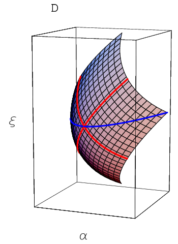 |
 | |
| (a) | (b) |
This spectral surface has a double-curve singularity and a pinch point, as in Figure 9. More natural extension of the idea in section 3, however, is to consider a space with a set of coordinate
| (162) |
To be more precise, the new space has a set of local coordinates , and a map is given by
| (163) |
This surface does not have a double-curve singularity or pinch point singularity. It is smooth, as in Figure 9 (a). The map is ramified at
| (164) |
This ramification divisor on is projected onto the branch loci . Repeating the same argument as in section 3, we expect that the zero-mode solution of the - multiplet is obtained as a single-component field on the desingularized spectral surface , and that the zero-modes are in one-to-one correspondence with holomorphic functions on modulo those that vanish on the covering matter curve , defined as the inverse image of from , . It is very natural to consider that this covering matter curve is the same thing as the covering matter curve introduced in [6]. We will show in the next section that they are indeed the same object.
4.3 Discriminant Locus and Spectral Surface
Let us take a moment here to study relation between the discriminant locus and (desingularized) spectral surface. Behavior of spectral surfaces around codimension-3 singularities has been analyzed in detail in the preceding sections. We will now take a brief look at the behavior of discriminant locus around codimension-3 singularities.
Discriminant locus is, by definition, where the elliptic fiber of F-theory compactification degenerates. Depending upon which 1-cycle of the elliptic fiber shrinks, a label is assigned to a discriminant locus (remember the monodromy, though) [35]. Degrees of freedom corresponding to various roots of - representations are obtained as string junctions [36] . When a pair of irreducible discriminant locus approach each other, therefore, an extra set of degrees of freedom corresponding to the junctions stretching between the two discriminant locus becomes massless, and charged matter fields are localized at the intersection—codimension-2 locus—called matter curves [28]. Intuitive picture of D7-branes in Type IIB string theory almost seems to hold for the discriminant locus in F-theory, except that the gauge group (including its deformation) can be type. To what extent is this intuition correct, when we look at the behavior of discriminant locus around codimension-3 singularities? To what extent is the converse true, or put differently, are there irreducible pieces of discriminant locus for individual matter curves (and matter multiplets) in different representations? We will see this in the following.3535 35 We will pay attention only to the local geometry of Calabi–Yau 4-fold around the (deformed) singularity locus, but we do not study how the overall elliptic fiber becomes around the codimension-3 singularities. This is because the geometry around the singularity locus is directly relevant to physics of gauge theory.
Let us begin with a codimension-3 singularity around which singularity surface is deformed to surface with singularity. Section 3 was dedicated for the study of this case. The non- component of the discriminant locus, denoted by in (6), is locally given by , and its behavior is shown in Figure 2. For the case with a complex structure given in (13), the discriminant locus consists of two irreducible pieces, and both of them are interpreted as D7-branes. Even in the case of generic complex structure, (28), may be understood as a recombination of two D7-branes. (See [5] for related discussion.) There is nothing particularly surprising or interesting, in the case type singularity is deformed to type. It is worth noting, the following, however. There is only one Hermitian conjugate pair of off-diagonal components in the irreducible decomposition of under the subgroup, which is a pair of fundamental and anti-fundamental representations. A spectral surface is associated with this pair of representations.3636 36 The spectral surface of -anti-fundamental representation is obtained by multiplying to the coordinate of that of the -fundamental representation. Local behavior of the discriminant locus in (see Figure 2 (b)) and the spectral surface in (see Figure 3) is exactly the same for this type of deformation.
We have also studied a codimension-3 singularity where type surface singularity is deformed to ; the type (c) codimension-3 singularity points of SO(10) models is an example of this type of deformation, and we studied this case in section 4.2.2. Around the codimension-3 singularity of deformation, the non- component of the discriminant locus is defined locally by
| (165) |
which was obtained from of (124) by dropping the higher order terms under the scaling specified in (155). . Its behavior is shown in Figure 10 (a).
 |
 | |
| (a) | (b) |
The discriminant locus in is irreducible around this codimension-3 singularity. At a generic point on the matter curve (codimension-2 singularity), the coordinate of depends quadratically on the normal coordinate of the matter curve (see Figure 10 (a)). This behavior is due to orientifold projection, and is known since 1990’s.
Just like in the case of deformation from to , there is only one irreducible off-diagonal component— representation—in the deformation of to . The defining equation of the spectral surface of this representation was (161), and the defining equation of the discriminant locus in and that of the spectral surface in are exactly the same, when is identified with . Although there is no “picture before orientifold projection” in generic F-theory compactification, the behavior of the spectral surface in Figure 9 gives an impression that the spectral surface can be regarded as such a picture (intersecting D7-branes) in generic F-theory compactification; the identification now looks like the orientifold projection.
One begins to see more interesting phenomena when studying deformation of surface singularity to . We already encountered this situation in section 4.1.2, where singularity is deformed to around the type (d) codimension-3 singularity of models. In order to find out the defining equation of the component of the discriminant locus around this codimension-3 singularity, we drop higher-order terms of of (50) under the scaling (56). It is
| (166) |
and factorizes. In the limit toward this codimension-3 singularity, the discriminant locus splits into two irreducible pieces, given by and by Their behavior is shown in Figure 10 (b). As a divisor, . The matter curve for the anti-symmetric representation of gauge group is regarded as the intersection , and the matter curve for the fundamental representation as the intersection .
There are three things to point out. First, there are three Hermitian conjugate pairs of off-diagonal irreducible components in the decomposition of -adj. representation. To each one of the pairs (and to each one of the irreducible pieces of matter curves) corresponds a spectral surface. The deformation of to has a Type IIB interpretation, as we already discussed in section 4.1.2, and the spectral surfaces carry information of the intersection of the two relevant D7-branes.
Secondly, we notice that the discriminant locus is irreducible, whereas the corresponding matter curve is split up into two irreducible pieces. Multiple irreducible components in the matter curve in does not imply at all that the discriminant locus has multiple irreducible pieces. On the other hand, there are corresponding irreducible pieces among the (desingularized) spectral surfaces.
Finally, the factorized form of the discriminant locus in (166) was obtained only after the higher order terms in the scaling was dropped. The two irreducible pieces and touch each other along a curve (see Figure 10 (b)), and they will reconnect to form a single irreducible piece under even a small perturbation coming from higher order terms in the scaling. Thus, the discriminant locus is a single irreducible piece for generic complex structure, even through the intersection sometimes have more than one irreducible components corresponding to matter curves of multiple representations.
At the end of the analysis in this section 4.3, let us look at the discriminant at the type (a) codimension-3 singularity of SU(5) models, where singularity is deformed to . The local defining equation is obtained just as we did above; we use the scaling (56) to drop higher order terms from (50).
| (167) |
We found that this does not factorize further into polynomials of local coordinates of , that is , and . Thus, remains irreducible even when zooming in to the codimension-3 singularity point. does not split to irreducible pieces for the two pairs of off-diagonal irreducible representations in (75). An intuition in Type IIB string theory that any charged matter multiplets are in one-to-one correspondence with systems of intersecting irreducible 7-branes breaks down here,3737 37 Although we sometimes find in recent literature on F-theory that irreducible pieces of matter curves are identified with intersection of discriminant loci, this is not always true in F-theory. if “7-branes” here mean 7-branes (discriminant locus) in . The spectral surfaces in , however, are defined separately for the pairs of off-diagonal irreducible components, and there remains a chance to extend the intuition in Type IIB string theory into generic F-theory compactification. This is done in the next section.
The irreducible nature of the component of the discriminant locus is not a new discovery, in fact. Geometry of F-theory compactification was studied in 1990’s, and was often treated as an irreducible piece as a whole. There was no reason to think that it is reducible, to begin with, unless phenomenological constraints are introduced. We have presented this detailed analysis of the behavior of discriminant locus around codimension-3 singularities, as a pedagogical introduction to the next section, where the spectral surfaces take center stage, not the discriminant locus.
5 Higgs Bundle in F-Theory Compactification
Massless charged chiral multiplets in low-energy effective theory are identified with global holomorphic sections of certain line bundles on (covering) matter curves [2, 3, 4, 5, 6]. Using the standard techniques in algebraic geometry, one can determine the sections over the (covering) matter curves completely. It is impossible, however, to determine even the number of independent massless modes without looking at the entire compact curves. Field theory local models discussed in [4, 5] and in earlier sections in this article may well be able to determine local behavior of zero-mode wavefunctions and calculate Yukawa couplings localized at codimension-3 singularities. But it is formulated on a non-compact base space , and covers only a local region in a discriminant for the low-energy gauge group. Wavefunctions are defined on the surface . In order to combine both techniques and calculate Yukawa couplings of zero modes in the effective theory, therefore, one needs to figure out the relation between the two descriptions of matters. One of them provides a global description based on curves, and the other is for a local description on surfaces!
An important hint comes from our observation in section 3. Although zero-mode wavefunctions are often multi-component fields on a surface , we found that they are better understood as single-component fields on (desingularized) spectral cover surfaces . We also found that the zero-mode wavefunctions are ultimately determined by holomoprhic functions (sections) on the spectral surfaces modulo those that vanish on the (covering) matter curves. After taking the quotient, the remaining degrees of freedom are only the sections on the (covering) matter curves! This must be the way the two apparently different descriptions are compatible.
With this motivation in mind, we lay down in section 5.1 a firm foundation for describing charged matter multiplets in F-theory using sheaves on spectral covers, not on matter curves. We do find indeed that quotients of holomorphic sections of sheaves on spectral cover is the natural way to describe charged matters in F-theory [that is, (186)], although in the end, this new description is equivalent to the one in [6], where charged matters are sections on curves. Spectral surface has never been used in study of F-theory compactification, but it turns out to be a key notion in generalizing such objects as D-branes and gauge bundles on them (or sheaves) in Calabi–Yau 3-fold in Type IIB compactification.
It is well-known that spectral surface is used in describing vector bundles in elliptic fibered compactification of Heterotic string theory [37, 38]. With the discovery of description of F-theory compactification using spectral covers, we have a new way to understand the duality between the Heterotic string and F-theory. In section 5.2 we find that charged matters can be identified as quotients of holomorphic sections of sheaves on spectral cover, also in Heterotic string compactification. Moduli of spectral surfaces and sheaves on them in both theories are directly identified in (201), a totally new way to describe the duality map. The new duality map improves the one developed in [31, 4, 6], and determines how to describe codimension-3 singularities in F-theory without a room of ambiguity.
5.1 Higgs Bundle, Abelianization and Group
5.1.1 -valued Higgs Bundle and Spectral Cover
Physics of gauge fields, charged matter and some of complex structure moduli of F-theory compactification can be described by the field theory formulation of [4, 5], once the field vev’s of a local model are determined properly from Calabi–Yau 4-fold and four-form fluxes. BPS conditions for background field configuration follows from vanishing vevs of the auxiliary fields , and [5]:
| (168) | |||||
| (169) | |||||
| (170) |
Thus, the gauge-field background defines a holomorphic vector bundle on with structure group . The (0,1)-part of the gauge field background can be “gauged-away” by complexified gauge transformation of . Thus, from3838 38 Remember that is still non-compact in this section. (170),
| (171) |
Although F-theory compactifications down to 5+1 dimensions are described by a 1-form field , instead of a 2-form , (171) remains true. The field background induces a map
| (172) |
Such a combination of is called -valued (canonical bundle valued) Higgs bundle in the literature. For example, see [39]. Supersymmetric compactification of F-theory, therefore, is described locally by the 8-dimensional field theory of [4, 5] with a canonical bundle valued Higgs bundle as a background.
For compactification down to 5+1 dimensions, where is a complex curve, the condition (169) becomes trivial. is a 1-form field, as mentioned, and the condition (168) becomes
| (173) |
A combination of (170) and (173) is called Hitchin equation.3939 39 Note that we adopt a convention throughout this article that gauge fields and are Hermitian, not anti-Hermitian. Historically, the Hitchin equation arose from dimensional reduction of anti-self-dual equation on a complex surface to a complex curve, which is also regarded as a generalization of the flat-connection condition on a complex curve [40]. Correspondence between Hermitian gauge field and satisfying (168–170) and an object of algebraic geometry , therefore, is regarded as a generalization (or dimensional reduction) of the works of Narasimhan–Seshadri [41], Donaldson [42] and Uhlenbeck–Yau [43]. Reference [40] proves the correspondence for the case is a curve.
For a given -valued Higgs bundle with a rank- structure group , -invariant homogeneous functions of of degree () can be constructed out of ; to be more precise, they are holomorphic sections of on :
| (174) |
When the structure group is , ’s () are symmetric homogeneous functions of eigenvalues of matrix valued of degree . For the case , as we encountered in sections 3, 4.1.1, 4.1.3 and 4.2.1, is the trace and determinant. Thus, and are , , and in these sections, respectively. If we were to consider full deformation of or singularity, with in (54) and with in (126) would have been the ’s for . The structure group is in the example of section 4.2.2, and and are the two sections of . These maps above are called Hitchin map and was introduced in [44]. Studies in the precedent sections correspond to the inverse process of the Hitchin map; it was to find whose reproduces coefficients of the defining equation of local Calabi–Yau geometry. One could also say that Calabi–Yau 4-fold provides a description of the same physics in terms of gauge invariants.
It is actually -valued -principal Higgs bundle, rather than -valued Higgs bundle in certain representation, that the geometry of Calabi–Yau 4-fold (and 4-form flux) determines. Certainly the irreducible decomposition of adjoint representation of under the subgroup in (8) yields only one off-diagonal component up to Hermitian conjugation in the case both and are of type, or both are of type. But, there are more than one if is type and is type, or in general. Geometry determines in , from which we can read the collection of eigenvalues of acting on individual irreducible components . From a -valued -principal Higgs bundle, all the -valued Higgs bundle in representation ’s are constructed.
For a given representation of , the collection of eigenvalues—spectrum—of can be extracted by defining a characteristic polynomial
| (175) |
The zero locus of this characteristic polynomial defines a surface , which is called spectral surface (or spectral cover in more general). The spectral surfaces are regarded as divisors of , the total space of canonical bundle , as we saw in sections 3 and 4 and as also known in the literature. Although it is possible to introduce a more universal object, like principal bundles that does not rely upon specific choice of representation , we will not do this in this article. There is such a need only for the cases with , where there are multiple irreducible components appearing in the irreducible decomposition, yet practically all we need is to deal with doublet and singlet representations of a Higgs bundle with structure group. Thus, there is no high demand for more abstract object; interested readers, however, are referred to [39].
We have already seen many examples of spectral surfaces of Higgs bundles in the preceding sections. The equations (43), (96) and (149) determine the spectral surface for the doublet representation of Higgs bundles with a structure group . The spectral surface given by (150) is for the representation . The field theory in section 4.2.2 has a Higgs bundle with the structure group , and the spectral surface for the vector representation of was given by (161).
5.1.2 Abelianization
It is known in the literature that a -valued Higgs bundle with a structure group or (in the fundamental representation ) has an equivalent description in terms of spectral data as long as satisfies certain conditions.4040 40 being “regular” is one of those conditions; see e.g. [47] for its precise definition. Precise conditions for or spectral cover seem to vary over the literature, and we are not sure of the precise set of conditions. Spectral data consists of a spectral surface , which is a divisor of , and a line bundle on it [44, 45, 39, 46]. From spectral data, , the holomorphic vector bundle on is recovered by
| (176) |
where is a degree- cover. Although the structure group of the theory on is non-Abelian, there is an equivalent description on the spectral cover that only involves a line bundle. This Abelianization makes our lives much easier.
The structure group of the -valued Higgs bundle was for the field theory local model of codimension-3 singularities of type (a) and (c1) in SU(5) GUT models and those of type (a) in SO(10) GUT models. For generic choice of complex structure moduli, the spectral surface is smooth and reduced, as in Figures 3 and 5 (ib), and extra care does not have to be paid. Although there is a subtlety of whether being regular or not, and uncertainty of how to determine from geometry of a Calabi–Yau 4-fold, not just their eigenvalues, we will rather take the spectral data as the starting point, and consider only Higgs bundles that are given by such spectral data. We need to deal with -valued Higgs bundle with the structure group for the field theory local model of the type (c) codimension-3 singularities, and the spectral surface is necessarily singular as we saw in Figure 9. We will come back to this issue later, and for now, we will discuss the simplest case where the structure group is .
References [48, 10] also introduce a notion of Higgs sheaf, which is a sheaf of -module on . A Higgs sheaf is constructed out of a Higgs bundle on in a procedure described there, and the spectral surface is regarded as the support of this sheaf . That is,
| (177) |
and . All the information of spectral data is simply described by the Higgs sheaf . Although we just refer to the literature [48, 10] and do not explain the procedure here, it is regarded as the inverse process of (176). Multiplying in (172) is equivalent to multiplying on the spectral surface, where is the coordinate of the fiber direction of the canonical bundle .
5.1.3 Zero-Modes and Group
In section 3, we had two observations. One is that zero-mode wavefunctions of chiral matter multiplets may be solved as a singled valued field configuration on the spectral surface , and the other is that the wavefunctions are ultimately determined by holomorphic functions on modulo those that vanish on the matter curve . We have yet to justify the first statement rigorously, however. We were not sure, either, sections of which bundle the functions correspond to, because our treatment of section 3 was only local, and furthermore, all the gauge-field background was ignored. Now, using the language of Higgs bundles and Higgs sheaves, however, we can address these problems.
It is known in Type IIB string theory [9] that open string zero modes from D7–D7 intersection are identified with groups. To be more precise, let us suppose that a D7-brane is wrapped on a divisor of a Calabi–Yau 3-fold with a gauge bundle on it, and another wrapped on a divisor with a bundle on it. Chiral massless multiplets in the open string sector from to are identified with
| (178) |
Those from to are identified with the group. Those extension groups are calculated by using spectral sequence, with
| (179) |
and are obtained by tensoring to cohomology sheaves of this complex
| (180) |
Zero modes of matter multiplets in F-theory are characterized by (22–25) in the field-theory formulation. For supersymmetric compactification, the wavefunctions of bosonic fields should be the same as those of fermionic fields . If one requires that an infinitesimal deformation from a BPS background still satisfies the BPS conditions (168–170), then the conditions on an infinitesimal deformation is exactly the same as the zero-mode equations. Thus, matter zero modes are regarded as infinitesimal deformation of Higgs bundle that still preserves the BPS conditions. Is this deformation characterized as an extension group? Is it possible to generalize the argument above, in a way suitable for F-theory compactification?
Inspired by the appendix of [10], we propose to generalize4141 41 A similar attempt was made in [4]. (178, 179) as follows: matter multiplets are identified with the extension groups
| (181) |
which is calculated by using spectral sequence from
| (182) |
Here, is the embedding of to through the zero section of the canonical bundle . Reference [10] discussed matter fields arising from D-branes sharing the same support in a Calabi–Yau 3-fold in Type IIB string theory, and an group on the normal bundle of , was used. We replaced by for F-theory. Higgs sheaves for bi-fundamental representations of Type IIB string theory in [10] will most naturally be generalized in F-theory to Higgs sheaves for irreducible components of the decomposition like (8). Thanks to the Abelianization, Higgs bundles with non-Abelian structure group can be dealt with as if they were 7-branes with Abelian background on them. If a line bundle is turned on on to break the GUT gauge group (such as SU(5) and SO(10)) to the Standard Model gauge group [49, 50]4242 42 See also [51, 52] for the preceding discussion in Type IIB language., then can be replaced by the line bundle.
To see whether this proposal is reasonable, let us obtain more explicit expressions for (182).4343 43 We assume that the spectral surface is well-behaved, and is different from trivial corresponding to . The extension sheaves are cohomology sheaves of this complex,
| (183) |
which is equivalent to
| (184) |
Now the support of all these sheaves is the spectral surface . It thus follows that
| (185) | |||||
| (186) | |||||
| (187) |
Here, is the matter curve, locus on where vanishes.
The spectral sequence already converges, because does not vanish only for . Thus, becomes the extension groups . Matter multiplets correspond to . Therefore, we obtain
| (188) | |||||
| (189) |
The holomorphic functions “” we encountered in section 3 exactly have these properties. They are locally holomorphic functions on the spectral surface , transform like or , which accounts for the tensor factor . What is really in one-to-one correspondence with the zero modes is the “functions” (in a local description) modulo those that vanish along , and (186) literally provides such a characterization of zero-mode matter fields. We will further see in section 5.2 that matter multiplets can also be characterized exactly in the same way in Heterotic string theory, and all these observations combined gives us a confidence in the proposal (181, 182).
We also find at the same time that the “” should be regarded as sections of . The “” part was not clear from the argument in sections 3 and 4, partly because we ignored gauge-field background coming from 4-form fluxes and partly because it was not clear how to treat the branch locus of the field theory local models of F-theory. By now, however, we can start from the spectral data in F-theory compactification, instead of Calabi–Yau 4-fold and 4-form flux on it. In the spectral data, there is nothing ambiguous in how to deal with the ramification locus.
5.2 Heterotic–F Duality Revisited
We have not used duality between the Heterotic string theory and F-theory so far. We have not even assume that Heterotic dual exists for a Calabi–Yau 4-fold compactification of F-theory. It is not difficult, however, to see how the duality relates both theories.
We have determined spectral surfaces of Higgs bundles from defining equations of Calabi–Yau 4-fold for F-theory compactifications. On the Heterotic theory side, where the Heterotic string theory is compactified on an elliptic fibered Calabi–Yau 3-fold on a common base 2-fold ,
| (190) |
a vector bundle within one of the factors is described by yet another spectral surface [37, 38]. When the elliptic fibration is given by a Weierstrass equation
| (191) |
with as the coordinates of the elliptic fiber, then the spectral surface of an bundle is given by
| (192) |
where () are sections of line bundles on , . The divisor on should be chosen so that the normal bundle of the F-theory compactification corresponds to [25, 26, 37, 34, 53]. The same notation are used in (49) and (192), because this is known to be the right duality map [30, 31, 4, 6]. Let us see in explicit examples in the following that the defining equations of the spectral surfaces of Higgs bundles in F-theory perfectly agree with those of spectral surfaces of vector bundles in elliptic fibered compactification of Heterotic string theory.
In the elliptic fibration given by (191), the zero section corresponds to . One can choose a local coordinate of the elliptic fiber around the zero section, so that and around the zero section. Around a type (a) codimension-3 singularity point of a theory with unbroken symmetry, where both and become small, the equation of the spectral surface (192) becomes
| (193) |
where now we only pay attention to a region near the zero section. This behavior of the spectral surface of an vector bundle in the Heterotic string theory is exactly the same as the spectral surface of Higgs bundle in (96) in F-theory. Similarly, the spectral surface of bundle in Heterotic string theory, , agrees perfectly with the spectral surface of Higgs bundle (149) of F-theory.
Reference [6] determined a defining equation of spectral surface of bundle for an vector bundle in Heterotic string theory, in a neighborhood of a type (c) codimension-3 singularity, . The spectral surface (161) of a Higgs bundle of F-theory perfectly agrees with the defining equation of in the appendix of [6] (after a few typos there are corrected).
The duality map between the vector bundle moduli of Heterotic string theory and a part of complex structure moduli of F-theory has been constructed by studying how the complex structure moduli of (del Pezzo 8) surface changes a flat bundle on . Now that we are familiar with the notion of Higgs bundle and its spectral data for F-theory compactification, we have a new channel (though essentially equivalent) of establishing a duality map: map the moduli parameters of both sides so that the spectral surfaces of vector bundles on elliptic fibration correspond to the spectral surfaces of Higgs bundle. The spectral surface in Heterotic side describes the behavior of Wilson line in the elliptic fiber direction. That is, degree- cover spectral surface over determines different values of Wilson lines (and ) for a given point in , where . The spectral surface in F-theory side describes different eigenvalues of at a given point in . The Heterotic–F theory duality simply replaces of Heterotic string theory by in F-theory and vice versa at each point on . The Calabi–Yau description of F-theory compactification extracts gauge invariants of the field-theory formulation through the Hitchin/Katz–Vafa map.
When a couple of irreducible components are involved in (8), which is usually the case, duality should be better stated as the correspondence between cameral covers of both sides. But this is still equivalent to equating the spectral surfaces for all the irreducible representations of those bundles that appear in (8), and we are not pursing in phrasing the duality in terms of cameral cover in this article.
The duality correspondence of zero-modes of both sides is also easier to see in the aid of spectral surfaces of Higgs bundle in F-theory side.4444 44 Since the zero-mode charged matters correspond to deformation of vector and Higgs bundles of both theory, the Heterotic–F duality (vector and Higgs bundle duality) for arbitrary structure group already implies the duality between charged massless matters, though. To begin with, let us remind ourselves how the zero-mode matter multiplets are identified in elliptic fibered Calabi–Yau 3-fold compactification of Heterotic string theory. Suppose that a vector bundle with a structure group is turned on , and that is given by a Fourier–Mukai transform of a line bundle on a spectral surface :
| (194) |
For now, we assume that the structure group of is not a proper subgroup of , but itself, and is irreducible and smooth. Fourier–Mukai transform of the bundle is represented by the original line bundle . In the irreducible decomposition (8) with and , there is an irreducible component where is the fundamental representation of . The zero modes chiral multiplets from this component is identified with a vector space
| (195) |
It has been customary, when we are to compare this expression with its F-theory dual counter part, to use the spectral sequence associated with the elliptic fibration (190):
| (196) |
where is a sheaf on , and we assumed that the bundle is non-trivial when restricted on a generic fiber of (190). The sheaf has a support only on the matter curve of bundle , and the localized sheaf on the matter curve is compared with (or translated into) line bundles localized on the matter curves in F-theory compactification [2, 3]. This is the traditional story.
Now that we also have spectral cover in F-theory side, however, there is another channel to compare the zero modes on both sides of the duality. Because the vector bundle on is given by a push-forward of a line bundle on , we can rewrite the sheaf , by following the argument of section 7.4 in [54]:
| (197) | |||||
Therefore, on the side of Heterotic string compactification, the zero mode matter multiplets from can be regarded as
| (198) |
holomorphic sections of a sheaf on the spectral surface , not on the matter curve . Zero modes are now characterized as holomorphic objects on the spectral surface (modulo redundancy as we see below) also in Heterotic string compactification.
The appendix A of [6] looked into the details of the sheaf . It is a sheaf on , although its support is the matter curve . It is characterized by this short exact sequence,
| (199) |
Here, is the ideal sheaf of the matter curve on the spectral surface , which is roughly speaking, holomorphic functions that vanish on . . All the three sheaves in the short exact sequence above are on the spectral surface . Local generators of the sheaf can be expressed as those of modulo image from . To be more explicit, the generators of in language of Čech cohomology are of the form [6]
| (200) |
where is a section of4545 45 Note that , and transform like sections of line bundles , and , respectively, and hence transforms as a section of . . The image from corresponds to “” that at least involves single power of the normal coordinate of the curve in . Explicit study of the structure of in [6] using Čech cohomology shows that is generated by ’s modulo the image from , and hence the characterization by (199) follows.
Simply tensoring to the argument above, we find that the zero-mode matter multiplets in representation are identified with global holomorphic sections of on the spectral surface , modulo those involving at least one power of normal coordinate of the matter curve. Now we will not need even a single word to see the dual correspondence with the characterization of zero mode matter multiplets in F-theory description, (186, 188). Alternatively, this agreement can be regarded as a justification of the proposal (181, 182).
5.3 Ramification and Four-form Flux
Spectral data are used on both sides of the duality between the Heterotic string and F-theory. The duality map is simply stated as
| (201) |
Not only the moduli of the spectral surfaces but also discrete as well as continuous data of the line bundles on both sides are identified. This novel way to see the duality allows us to bypass the complicated discussion involving -fibration and its blow up to -fibration, and (projected) cylinder map in [31, 4, 6] in mapping the discrete data of into F-theory.
This observation goes beyond a discovery of academic interest, and brings a practical benefit. The spectral cover is generically ramified in Heterotic and F-theory compactifications alike. References [4, 6] used the Heteroic–F theory duality to study how the four-form flux determines the sheaves/bundles on the (covering) matter curves for F-theory on a Calabi–Yau with generic complex structure. But, there was one weakness in the argument. The duality map of the discrete data of through del Pezzo fibration assumes that there is a well-defined choice of independent basis of 2-cycles of del Pezzo fiber. But, two 2-cycles of del Pezzo fiber become degenerate where the spectral surface ramifies, and it is not obvious how to choose independent 2-cycles at the branch locus. This weakness of the argument in [4, 6], however, is overcome under the new duality map. Here, we do not have to go through del Pezzo fibration, and no ambiguity arises in translating (copying) the line bundle from Heterotic string to F-theory, even along the ramification locus of the spectral cover.
The line bundles corresponding to a bundle with structure group has a description
| (202) |
where is the ramification divisor of , and another divisor (allowing half integral coefficients) of . This result is known to most physicists through [37], where arises as a part of spectral data for Heterotic compactification. The part in Heterotic string corresponds to four-form flux in F-theory [31, 4, 6]. The separation between the piece and the rest also appeared in mathematical literature describing abelianization of Higgs bundles; see [39] and references therein. Thus, the separation between the part and the rest goes hand in hand on the both sides of the duality.
In order to understand physics associated with codimension-3 singularity of F-theory compactification, it turns out that it is best to study the effects of and separately. In the following, we will work on issues associated with piece in section 5.3.1 and those with (equivalently the four-form flux) in section 5.3.2.
5.3.1 Ramification
Using the expression (202), the zero-modes from the fundamental representation of (a relevant local part of) vector/Higgs bundle is rewritten as [2, 3, 6]
| (203) |
maps and are those in the diagram below:
| (204) |
Some of the objects and maps in this diagram have not been used so far, but they will appear later on. Reference [2] showed by using the adjunction formula that
| (205) |
and hence the Serre duality accounts for the anticipated relation
| (206) |
We have nothing more to add for the cases with structure group, except that the spectral surface can be defined intrinsically from Calabi–Yau 4-fold for F-theory compactification, and that the same logic as in [2] can be used to show (205) even for F-theory compactification without Heterotic dual.4646 46 A proof for (205) in F-theory compactification without Heterotic dual was obtained in [6], by counting the number of type (a) codimension-3 singularity points. We find the argument here more elegant, however.
Spectral surfaces for the matter of SU(5) representations and for those of SO(10) vect. representation are not smooth everywhere along the matter curve, even for the most generic choice of complex structure moduli of F-theory compactifications. (120) has a double curve singularity around type (d) codimension-3 singularity points, and in (161) has a double curve along and a pinch point singularity at around type (c) codimension-3 singularity points. Those matter multiplets are both from bundles in Heterotic string compactification, and Ref. [6] studied the structure of the sheaf . The sheaf is represented by a pushforward of a line bundle on the desingularization ,
| (207) |
In the context of F-theory compactifications / Abelianization of Higgs bundles, it is just natural from D7-brane interpretation to consider desingularized spectral cover in (121) and gauge bundles on individual irreducible components. Reference [44] already points out the need of resolving double-point singularity on the spectral cover when the structure group is when is a curve; the structure group around the type (c) codimension-3 singularities in SO(10) GUT models was , and this is one of the cases Hitchin’s observation is applied. Now, the double-curve singularity has to be resolved. The necessary resolution of the double curve also resolves the pinch-point singularity, and that is .
For any representations of vector/Higgs bundles, the line bundle on should have a factor , apart from the one coming from (or from three-form potential in F-theory). Here, is the ramification divisor associated with . By repeating the same argument as for (205) and noting that the covering matter curve in is defined as the zero locus of the coordinate [6], one finds that
| (208) |
Here, is a map from the covering matter curve to passing any routes in (204). Using this relation and Serre duality on the covering matter curve , it is now easy to see the relation analogous to (206) for the number of multiplets in -5 representation. This observation greatly simplifies the argument4747 47 References [54, 55, 6] eventually arrived at a divisor on ; here, is the ramification divisor of . See [6] for notations. It is possible to understand intuitively that this divisor corresponds to as follows. The desingularized spectral surface consists of points , where both and are points in that are mapped to the same point in , and stands for the group-law summation. When a layer of containing either or is ramified over , so is . The only exception is the case when the layers of containing and locally form a degree-2 ramified cover over . The spectral surface is not ramified in this case. This is why the component has to be subtracted to obtain from . in [54, 55, 6].
Reference [6] found that the charged matter zero modes of F-theory are global holomorphic sections of line bundles on covering matter curves, ; the line bundles on are described by their divisors, and the divisors were determined by using the Heterotic–F theory duality. The divisors have support on codimension-3 singularity points of F-theory. The coefficients of the divisors at these singularities were determined by the duality, but an explanation intrinsic to F-theory was not found, and remained an open problem. Now a complete answer to this question is available. Codimension-3 singularity is formed whenever the ramification divisor of (desingularized) spectral surface intersect the (covering) matter curve, and the piece of always leaves a contribution to the divisor on the (covering) matter curve. The coefficients at the codimension-3 singularities are determined purely from the ramification behavior of the (desingularized) spectral surfaces of the Higgs bundle of F-theory compactification.
Now that all the subtleties associated with ramification / branch locus have been clarified, we can fill-in the missing details of our observation in section 3. The zero-mode equations (22–25) on for an irreducible component are for a set of fields with components. We found in section 3, however, that it is possible to write down an equivalent set of equations on the desingularized spectral surface , where we only need a single component of . This idea now seems very convincing, because charged matter zero modes are characterized as holomorphic sections of sheaves on the (desingularized) spectral surfaces, modulo redundancy, both in F-theory and Heterotic string theory. Covariant derivatives in the set of equations should involve gauge fields, and the gauge field backgrounds are determined from the line bundle . This line bundle is determined by half-the-ramification-divisor twist of and by three-form potential background.
5.3.2 Four-form Flux
In this section 5.3.2, we address two issues associated with four-form flux background, or almost equivalently in (202). This part is digression in nature, and readers may skip and proceed to section 6.
The first goal we achieve in this section 5.3.2 is to obtain better understanding of what is really going on in the presence of both the ramification divisor and 4-form flux in (202). The second objective is to illustrate how one and the same four-form background determines gauge field backgrounds for fields in different representations.
supersymmetry is preserved when a 4-form flux background in a Calabi–Yau 4-fold is primitive and is in the (2,2) part. One needs to know global geometry of in order to determine the whole variety available in . For the purpose above, however, we only need illustrative examples, and hence we will use a (topological) form of that has been known in elliptic-fibered Calabi–Yau 3-fold compactification of Heterotic string theory.
In Heterotic string compactification on an elliptic fibration, a “divisor” on a spectral surface of an vector bundle in (202) has to satisfy
| (209) |
We can choose
| (210) |
as a solution to (209) [37]. Here, are those appearing in the defining equation of the spectral surface (192), and for SU(5) GUT models and for SO(10) GUT models. Although we use a language in Heterotic string compactification and deal with the (spectral surface of) full rank- vector bundle on, it will not be difficult to extract the rank-1 or rank-2 part relevant to the matter curve and codimension-3 singularities. Because of the duality relation (201) the whole story below is for F-theory compactifications as well.
Let us first focus on a region around a type (a) codimension-3 singularity point of SU(5) / SO(10) GUT models. There, only rank-2 part is relevant, and the relevant part of the spectral surface is defined by (96, 149), which are reproduced here as
| (211) |
where and , and can be chosen as a set of local coordinates on the spectral surface. The divisor in (210) can be expressed locally as
| (212) |
When a divisor is locally given by , where is a rational function, a line bundle has a description in terms of gauge field, with its singular component given by4848 48 This singular component does not depend on the choice of , because for another choice , should be holomorphic, and neither zero or infinite.
| (213) |
Thus, for in (210, 212), the singular component of the gauge field is
| (214) |
We will be satisfied in this section 5.3.2 only with following this singular component4949 49 This singular component disappears in local trivialization frame of a line bundle, and smooth component remains. We still use only the singular component, because it is easily determined, and because just the singular component is sufficient in illustrating a topological configuration of the corresponding four-form flux around type (a) codimension-3 singularity points, as well as illustrating how the gauge field backgrounds for 2 and representations are related. around the type (a) codimension-3 singularities.
It is also possible to obtain matrix representation of the gauge field background for the field-theory formulation on . The coordinate values of the degree-2 cover is
| (215) |
as functions of local coordinates of . Using this expression for , above can be rewritten. If we denote for branch as
| (216) |
then
| (217) | |||||
| (218) |
becomes negative of what it is after going around the branch locus . Noting that the topological 2-cycle also becomes negative of what it is around the branch locus (as we saw in section 3), we see that the 3-form potential—product of and the 2-form to be integrated over the 2-cycle---is invariant under the monodromy.5050 50 Although a massless vector field for this Cartan part is absent in the effective theory below the Kaluza–Klein scale because of the monodromy, topological background flux can be introduced in this Cartan part. These two things should not be confused.
The gauge field background for the [resp. ] representation is given by representation of what we found above. Therefore,
| (219) |
It is needless to say that , corresponding to the fact that
| (220) |
contains a singlet of the structure group .
6 Yukawa Couplings
For Heterotic string compactification on a Calabi–Yau 3-fold , the chiral matter multiplets correspond to independent basis of a vector space
| (221) |
where the vector bundle is a part of and is not necessarily assumed to be irreducible. The Heterotic string theory has a superpotential
| (222) |
and Yukawa interactions are calculated by substituting into the above superpotential. In Type IIB Calabi–Yau orientifold compactification with D7-branes wrapped on holomorphic 4-cycles, the chiral multiplets are identified with certain global holomorphic sections on vector bundles (often line bundles) on complex curves of D7–D7 intersection, and Yukawa couplings of three chiral multiplets are generated at points where three stacks of D7-branes intersect. Since the Type IIB string theory is formulated so that it can compute any short-distance physics processes, Yukawa couplings can be calculated although D7-branes and their intersection curves form a codimension-3 singularity there.
References [4, 5, 6] clarified how chiral matter multiplets are characterized in terms of geometry in F-theory, and the preceding sections of this article elaborate on it. One of the most important motivations of studying F-theory compactification, as opposed to limiting to Type IIB Calabi–Yau orientifold compactification, is that Yukawa couplings of the form (53) can be generated. However, it has been a long time puzzle how to calculate Yukawa couplings of low-energy effective theory for a given geometry for compactification.
It is not that we do not know anything about Yukawa interactions in F-theory. F-theory is regarded as the small fiber limit of M-theory compactification on an elliptic fibered manifold. The algebra of vanishing cycle suggests what kind of Yukawa couplings can be generated [1]. We have also learnt that such Yukawa couplings can be attributed to codimension-3 singularities [6]. In the absence of a microscopic quantum formulation of F-theory, however, it appears to be difficult to find a way to calculated Yukawa interactions that are associated with singularity points.
The field-theory formulation of “particle physics sector” of F-theory initiated by [4, 5], however, offers a solution. The singular geometry is encoded as a background of a 8-dimensional gauge theory the and microscopic aspects (quantum UV completion of F-theory) may well be dealt with by -(or -)expansion. It has a superpotential [4, 5] 5151 51 The F-term part of the BPS conditions (169, 170) follows from the superpotential (223). The F-term scalar potential from (223) gives rise to quartic interactions among zero mode scalar fields in effective field theory below the Kaluza–Klein scale. This interaction corresponds to the fact that not all the infinitesimal BPS deformation (massless modes) can simultaneously turned on together to obtain finite BPS deformation of the Higgs bundle. Yukawa interactions are regarded as the supersymmetrization of this quartic interactions.
| (223) |
which is the F-theory counter part of the Heterotic result (222) and of type IIB result
| (224) |
in Type IIB string theory. In this section, we will study how (223) can be used to calculate Yukawa couplings of charged matter multiplets in most generic compactification of F-theory.
6.1 Combining Local Models with Different Gauge Groups
The first step of the process of calculating the Yukawa couplings is to identify the zero mode chiral multiplets. This cannot be done without looking at the entire compact discriminant locus . The zero modes are
| (225) |
global holomorphic sections of line bundles along the covering matter curves, which are loci of desingularization of the spectral surfaces. The divisor is the ramification divisor of over , but only a geometry of along is needed to determine this divisor restricted on . See [6] for more details.5252 52 All topological aspects of elliptic fibered Calabi–Yau 4-fold , , and four-form flux on have to be arranged properly, so that there are three independent global holomoprhic sections corresponding to left-handed quark doublets etc., and there is just one corresponding to up-type Higgs doublet, for example. Finding an explicit example of topological choice of , , and four-form flux right for the minimal supersymmetric standard model is not the subject of this article. We just assume that there are the right number of independent global holomorphic sections for certain choice of geometry, and we just move on.
By definition, line bundles have descriptions of local trivialization, where holomorphic sections are expressed as holomorphic functions in any local patches covering the curve.5353 53 At the same time, the singular component of the gauge-field background that we discussed in section 5.3.2 also goes away when we take the trivialization frame. Zero modes, and hence the global holomorphic sections are cast into holomorphic functions in any given local patches within . Let us take a basis of the vector space (225) for representation , and denote the holomorphic function expression of in a trivialization patch as .
The Yukawa couplings of charged matter multiplets are expected to be generated around points of codimension-3 singularities. Thus, one chooses a local patch around a given point of codimension-3 singularity in , so that the intersection of and (covering) matter curves is contained in a trivialization patch on the (covering) matter curves. For such a given local patch an appropriate field-theory local model with an appropriate gauge group and background is chosen from those in sections 3 and 4. The zero-mode wavefunctions are determined on a patch of desingularized spectral surface from the holomorphic functions . The holomorphic functions on the curve are regarded as holomorphic functions on (desingularized) spectral surface , modulo those that vanish along the curve . We found in sections 3, 4 and the appendix B that the zero-mode wavefunctions are smooth on the desingularized spectral surfaces. From knowing a wavefunction on the desingularized spectral surface, a wavefunction on is constructed. This wavefunction becomes multi-component, if is a multi-degree cover. Note that the same gauge field configuration has to be used for different representations in determining the wavefunctions in a given patch . We have already studied in sections 4 all types of codimension-3 singularities that appear in F-theory compactifications for SU(5) or SO(10) models, and found that zero-modes are either in the Gaussian form [8, 5] (when the fields are in linear Abelian background) or in a form studied in section 3.2 and the appendix B when fields are in the doublet background. This is how the field-theory local models on complex surfaces with specific choices of their own (often non-Abelian) structure groups are combined by global descriptions of zero-modes on compact complex curves given in terms of (Abelian) line bundles.
Such wavefunctions are inserted into (223), and integration should be carried out over the patch . The wavefunctions are expected to damp very quickly in a direction normal to matter curves even in the doublet background, as we saw in sections 3, 4 and the appendix B. If the size of the discriminant locus is sufficiently large compared with the width of the exponentially decaying zero-mode wavefunctions,5454 54 We will discuss whether this assumption is reasonable late on. the integration is likely to be concentrated around the points of codimension-3 singularity. Because of the term in , three wavefunctions can be plugged in. When the wavefunctions for , and () are plugged in, the commutator algebra of the structure group determines what kind of Yukawa couplings are generated, and the integration yields a contribution to the Yukawa couplings associated with the point of codimension-3 singularity .
6.2 Yukawa Couplings from a Single Codimension-3 Singularity Point
There is nothing more to add in this article about Yukawa couplings generated around a codimension-3 singularity point where the structure group of its local model is Abelian, and three matter curves pass through the point.
What we call type (d) codimension-3 singularities of SU(5) models satisfy this criterion for generic complex structure of Calabi–Yau 4-fold. That is where Yukawa couplings of the form (100)—down-type Yukawa and charged lepton Yukawa couplings in Georgi–Glashow SU(5)—are generated. Three matter curves run through any given point of type (d) codimension-3 singularity, and wavefunctions are Gaussian in the normal directions of the matter curves for all three matter curves. One just needs to calculate the overlap of Gaussian wavefunctions. Because of the algebra, one wavefunction is picked up from one of the two branches of the (covering) matter curve of representation, and another from the other branch. If the width of the Gaussian profile is sufficiently small compared with typical radius of the compact discriminant locus , then the Yukawa coupling from a given codimension-3 singularity point is approximately given by [5]
| (226) |
where are values of those holomorphic functions at the codimension-3 singularity point, and is a numerical constant that depends on the width parameter of the Gaussian profile and the angle of the intersection of the curves.
The Yukawa coupling of the form (53)—up-type Yukawa couplings of Georgi–Glashow SU(5)—or (125) in SO(10) models, on the other hand, are expected to be generated at type (a) codimension-3 singularity points of those compactifications. For generic choice of complex structure, only two matter curves run through the codimension-3 singularity points. The Yukawa couplings at such singularities or even the field theory local models for this type of codimension-3 singularities have not been studied so far. Since the discussion proceeds exactly the same way for the Yukawa couplings (53) for SU(5) models and (125) for SO(10) models, we will only discuss the SU(5) cases in the following.
The first thing to check is the algebra. A local geometry around a type (a) codimension-3 singularity point of SU(5) models is a family of deformed singularity. The irreducible decomposition of algebra in terms of subgroup is given in (75). If we denote the generators of in the component as , the ones in the component as , and the ones in the as , then
| (227) |
and hence
| (228) |
Here, are indices labelling doublets, and are SU(5) indices. The totally anti-symmetric tensor comes from the structure constant of Lie algebra. The doublet indices are contracted in order to extract singlet part out of
| (229) |
The -valued gauge field on is expanded as
| (230) | |||||
Here, is the -doublet wavefunction in for a zero mode , and the corresponding complex scalar field in the SU(5)-10 representation in the low-energy effective theory. and are zero-mode wavefunctions in the and representations of the structure group , and and their corresponding scalar fields in the effective theory. Another field is also expanded similarly. Because of the structure constant of , the up-type Yukawa couplings in Georgi–Glashow SU(5) models have a contribution
| (231) |
from a local region around a type (a) codimension-3 singularity point .
Let us take a set of local coordinates on , so that and . Then, the -singlet wavefunction of the Higgs boson vanishes in the component, and the other two components are localized along the matter curve . The wavefunction in the remaining two components decay as in a Gaussian form . Therefore, the behavior of the quark wavefunctions is relevant to the overlap integration (231) only in the large and small region, which is just the behavior already studied in sections 3, 4 and the appendix B. The -doublet wavefunctions of quarks vanish in the component at the leading order, and , and these two components decay as for large . Using this information, we see first that the first term in (231) vanishes at the leading order. The second (and the third) term does not vanish; neither nor vanish, and they are different only in sign. Being multiplied by the anti-symmetric structure constant , the last two terms of (231) give rise to non-vanishing unsuppressed contributions to the up-type Yukawa couplings. The overlap integration is concentrated around the type (a) codimension-3 singularity point at , because of the exponentially decaying product of wavefunctions .
References [5, 7] considered that there are always three matter curves intersecting at a point of enhanced singularity, and the up-type Yukawa couplings were considered to be generated only at triple intersection of matter curves. This is why [7, 12, 11] were led to consider that complex structure has to be chosen so that the matter curve of -10 representation has a double point right on the matter curve of - representation, and diagonal entries of the up-type Yukawa matrix are generated. As we saw above, however, for generic choice of complex structure moduli in F-theory compactifications, the type (a) codimension-3 singularity points of SU(5) models have only two intersecting matter curves, and yet the up-type Yukawa couplings (53) are generated. In the evaluation of the overlap integration above, generation indices did not play an important role. The argument is valid for diagonal and off-diagonal entries alike.5555 55 In Heterotic string compactification, the up-type Yukawa couplings comes from (232) where is a rank-5 (rank-4 for SO(10) models) vector bundle turned on on a Calabi–Yau 3-fold . In F-theory compactification, we do the same thing; vector bundles on are replaced by Higgs bundles on , and that is basically it. In Heterotic string compactification, one is not usually worried whether diagonal entries are generated or not. It is dangerous, though, to rely too much on such an intuition coming from duality, because even in a compactification described by both theories, Heterotic string and F-theory provide good descriptions of different parts of the moduli space. Thus, such a specific choice of complex structure with the double points of the -10 representation matter curve on the - representation matter curve is not required from phenomenology. Just a generic complex structure is fine in obtaining a large third generation Yukawa coupling of the up-type quark.
If one assumes that the wavefunction and vary only slowly on their matter curves around , then the same argument for the down-type Yukawa couplings is applied to the up-type Yukawa matrix. Just like in (226), the up-type Yukawa matrix is rank-1 at the leading order.5656 56 If the matter curve of the - representation is irreducible (and hence all the three independent zero modes are localized on it) and has a double point at , so that a triple intersection of matter curves is realized by a self-pinching irreducible matter curve of 10 representation, then the up-type Yukawa matrix of is given by (233) at the leading order. Note that and are projected to the same point , but they are different points on the covering matter curve, where the double point of the matter curve is resolved. Holomorphic sections on the two irreducible branches of the matter curve of the 10 representation around the double point are independent (see discussion in p. 4.1.1 if necessary; are values of at , and those of ). Certainly one can choose a basis of the three quark doublets so that around on the branch of the covering matter curve, and the basis of the three anti-up-type quarks similarly on the branch. The first term of (233) does not vanish only in the (3,3) entry in this basis, and is clearly rank-1. The second term is also another rank-1 matrix, and is generically different from the first one. Thus, the situation here predicts a rank-2 up-type Yukawa matrix at the leading order.
The Yukawa matrix (226) and its up-type counter part are both rank-1, whereas the Yukawa matrices are supposed to be rank-3. Reference [11] proposed that there are only one pair of type (d) and type (a) codimension-3 singularity points, and in the SU(5) discriminant locus, and showed that the derivative expansion of wavefunctions5757 57 Reference [56] also discussed the derivative expansion of wavefunctions as one of the origin of the hierarchical mass eigenvalues. around and distortion of wavefunctions due to the presence of fluxes give rise to deviation from the rank-1 form, suppressed typically by powers of . Although the discussion in [11] explicitly relies on codimension-3 singularities at a triple intersection of matter curves, the idea of controlling the corrections from derivative expansion and flux distortion is more general, and Froggatt–Nielsen-like pattern will be expected also for the up-type Yukawa matrix generated around a type (a) codimension-3 singularity with only two matter curves intersecting normally. Details of the mass-eigenvalue pattern may or may not be different from the prediction of [11]. This is an interesting question, because the hierarchy between the up-quark and top-quark Yukawa couplings is larger than that between the down-type and bottom-quark Yukawa couplings, but we leave it as an open problem.
There is another contribution to Yukawa matrices, even when there is only one codimension-3 singularity point of a given type. To see this, we begin with the following observation. As noted in [7], the GUT unification gauge coupling and the GUT scale are given by
| (234) | |||||
| (235) |
where is the typical size of , the string length and “typical” dilaton vev. The GUT symmetry breaking is assumed to be due to fluxes in the U(1)Y direction, and hence the GUT scale is identified with the Kaluza–Klein scale. Here, Type IIB language is used just to make a crude estimate of the parameters of compactification. The definition of above is ; factors such as are ignored in the equations above, but that would not significantly affect the estimate of . In F-theory, however, it is not actually clear what this means. Since we are interested in F-theory configurations that have enhanced singularity of exceptional type, some mutually non-local 7-branes are involved. The dilation vev , therefore does not remain constant because of monodromy, and in particular, it cannot remain much smaller or much larger than unity. Setting as a crude approximation, and using experimentally inferred value , we conclude that
| (236) |
We have so far assumed that the zero-mode wavefunctions are localized along the matter curves quite well. To what extent, however, is this assumption correct? Wavefunctions are in the Gaussian profile in the normal directions of the matter curves (except at codimension-3 singularities), and its width parameter is given by the , where is the coefficient of , and is the normal coordinate. If the typical value of is of order unity in unit of , then . Gaussian tails of wavefunctions on near-by matter curves have significant overlap, and the picture we have assumed is not actually correct.
It is not clear what the right choice of “string unit” is; instead of might be the right characteristic scale of “stringy” regime. If the coefficient is typically of order unity in unit of , then . Reference [56] showed that the overlapping tails of Gaussian wavefunctions alone generate hierarchical Yukawa eigenvalues of the right amount of hierarchy for . One can ignore this contributions from overlapping Gaussian tails, only when . Since the set-up in [56] is not exactly the same as the situation here, it is a little dangerous to use the criterion literally, and conclude that is safe. In principle, typical values of relatively to can be studied by flux compactification. Such study will tell us whether this contribution can be ignored, or rather accounts for the hierarchical Yukawa eigenvalues.
Acknowledgements
This work is supported by Global COE Program ”the Physical Sciences Frontier”, MEXT, Japan (HH), a Grant in-Aid No. 19540268 from the MEXT, Japan (TK), PPARC (RT), and by WPI Initiative, MEXT, Japan (TW).
Appendix A Field Theory Lagrangian for 7-Branes
Reference [5] obtained a local field theory Lagrangian of 8-dimensions, which can be used to study localization of matter multiplets on 7-branes as well as how Yukawa couplings are generated. In this appendix, we quote the Lagrangian [5] with corrected coefficients, along with detailed explanation of conventions.
Conventions
The Lagrangian is described in terms of a vector multiplet and chiral multiplets and . takes its value in ; is real and generators of Lie algebra are in a Hermitian representation. and , on the other hand, take their values in .
We stick to all the conventions adopted in [57], and in particular, the metric is in space directions. is real as in [57], as opposed to the convention in [5], so that the SUSY transformation rule in [57] can be used without modification. The covariant derivatives are of the form
| (237) |
and hence field strength is
| (238) |
Holomorphic coordinates () are introduced in the internal 4-dimensions. Four real local coordinates are combined into and . Derivatives and gauge fields in the holomorphic coordinate system are defined by
| (239) |
| (240) |
Covariant derivatives are of the form and (). The lowest (complex scalar in ) components of chiral multiplets are identified with the gauge fields defined as above, and hence they have unambiguous normalization now.
Using the local holomorphic coordinates (), Kähler metric is given by
| (241) |
where is Hermitian, and the Kähler form by
| (242) |
so that
| (243) |
is the volume form. Euclidean metric corresponds to taking .
Differential forms can be used in writing down the Lagrangian. Following the convention of [5],
| (244) |
| (245) |
Note that there is no inserted in the definition of these (2,0)-forms. On the other hand, we use a notation
| (246) |
| (247) |
Here, , as before, where can be any one of , in (239, 240) and .
Lagrangian
All the conventions are fixed, and now one can follow the logic of the appendix C of [5] to obtain a local field theory Lagrangian of 8-dimensions. Purely bosonic part is
| (248) | |||||
and a part bilinear in fermions is given by
| (249) | |||||
The chiral multiplet appears in this Lagrangian only in a form , where is a complex-valued parameter. This reflects the fact that we have not fixed a normalization of yet. Different value of corresponds to different normalization of , and does not have any physical meanings. stands for for a representation of , and its Dynkin index.
Among the various terms in the Lagrangian (248–249), those involving correspond to in (C.13) and those proportional to to in (C.17) of [5]. Terms involving only or correspond to in (C.18) and in (C.10) of [5], respectively, and those involving to in (C.9) of [5]. The relative normalization among those four groups of terms are determined by requiring that the gauge-field kinetic terms becomes invariant. By integrating out auxiliary fields and from (248), one finds indeed that the gauge-field kinetic terms are
| (250) | |||
where the second line comes from integrating out , and the third line from . All these terms are nothing but invariant , where .
BPS Conditions
In the process of completing square for , and , one also finds that
| (251) | |||||
| (252) | |||||
| (253) |
Here, of a (2,2)-form is defined by . Background field value of and has to be chosen so that all of , and vanish. Vanishing means that the gauge bundle can be chosen as holomorphic vector bundles (vanishing ). Vanishing also says that , that is depends only holomorphically on complex coordinates ().
Appendix B Zero-Mode Solution in the Doublet Background
This appendix is dedicated to study of zero-mode wavefunctions. From the zero-mode equations (24, 25),
| (254) |
here we simply write as . is assumed to be diagonal here, and ’s are diagonal entries of . Substituting above into another zero-mode equation (22), we obtain
| (255) |
where a new set of coordinates are introduced just for better readability.
In the main text, we encountered cases with , and
| (256) |
where the coordinate here corresponds to in (29). The doublet background also determines the zero-mode wavefunctions of multiplets of GUT models around type (a) codimension-3 singularities, those of multiplets of GUT modes around type (c1) codimension-3 singularities, and those of multiplets of GUT models around type (a) codimension-3 singularities. The zero-mode wavefunction is known to decay in a Gaussian profile in the case is linear in a single coordinate, but it is not easy to find a solution for cases with general . In this appendix, we will find a zero mode solution under the doublet background that is valid in a region of sufficiently small .
The background field vev in (256) has an expansion
| (257) |
This is a -expansion, and leading order terms should give a good approximation to for sufficiently small . The leading order solution of (255) is determined by the condition
| (258) |
where for the leading order of the doublet background. ( for the case.) We drop dependence from for now, because does not depend on the coordinate at the leading order. Now the solution is obtained by series expansion in ; one can see explicitly that the following series
| (259) | |||||
| (260) |
satisfy (258). Thus, the leading-order solution should be given in a linear combination
| (261) |
We are interested in a solution localized along the matter curve, which is now . To see the constraint imposed on , , and for a localized solution, let us study the asymptotic behavior of the solutions above. To this end, it is important to note that the series expansion form of and is written by generalized hypergeometric functions,
| (262) |
For the case of our interest, is relevant, and , and . Asymptotic behavior of the generalized hypergeometric functions for large was studied in [58]:
| (263) | |||||
The coefficients of the asymptotic expansion () do not depend on , the first two of which are
| (264) |
where . Looking at the leading order term in the asymptotic expansion, we see that all of and grow exponentially for large :
| (265) | |||||
| (266) |
where we used , and overall coefficients are ignored. In order to cancel this exponential growth to obtain a localized zero-mode solution, and with have to be employed and their coefficients have to be properly adjusted. Requiring that the zero-mode solution does not have a pole at , and it is either single valued5858 58 Remember that there is an monodromy exchanging and . is a coordinate introduced in (41). in ,
| (267) |
is the only possibility. Therefore, the zero-mode solution is given by
| (268) |
To see that this solution is really localized around small , we need to note the following. The coefficients in the asymptotic expansion (263) are those appearing in the asymptotic expansion [58]5959 59 For the case , , and . In this case, for all , and the terms become the Gaussian-form wavefunction.
| (269) |
With a change of variable , one can show that
| (270) |
Therefore, , and the ratio are all the same for any . As we set the coefficients and so that the -term of the growing exponentials cancel, all the higher order -terms multiplying the growing exponential also cancel between and . Only the decaying exponential part survives because of the phase factor in the second line of (263), and the zero-mode solution behaves asymptotically as
| (271) |
at large at the leading order. Compared with the case , when the zero-mode wavefunction decays as the standard Gaussian profile, , the wavefunction decays more slowly, , when . The zero-mode wavefunction is still localized along the matter curve characterized by even in cases where .
For small , this solution behaves as
| (272) | |||||
| (273) |
The part6060 60 The subscript 0 means that this is a solution at the leading order. of the zero-mode wavefunction is obtained by using (254).
| (274) | |||||
| (275) |
Note that the zero mode solution behaves much better when it is expressed on the 2-fold covering space (with coordinate ). No half-integral power of or appears in in (273), and an apparent singularity in is gone in (275). This is another indication6161 61 For the other indication associated with the monodromy of the fields around codimension-3 singularity points, see the main text. that the covering space , rather than the base space , is where the zero-mode wavefunctions sit in the doublet background.
References
- [1] R. Tatar and T. Watari, “Proton decay, Yukawa couplings and underlying gauge symmetry in string theory,” Nucl. Phys. B 747, 212 (2006) [arXiv:hep-th/0602238].
- [2] G. Curio, “Chiral matter and transitions in heterotic string models,” Phys. Lett. B 435, 39 (1998) [arXiv:hep-th/9803224].
- [3] D. E. Diaconescu and G. Ionesei, “Spectral covers, charged matter and bundle cohomology,” JHEP 9812, 001 (1998) [arXiv:hep-th/9811129].
- [4] R. Donagi and M. Wijnholt, “Model Building with F-Theory,” arXiv:0802.2969 [hep-th].
- [5] C. Beasley, J. J. Heckman and C. Vafa, “GUTs and Exceptional Branes in F-theory - I,” arXiv:0802.3391 [hep-th].
- [6] H. Hayashi, R. Tatar, Y. Toda, T. Watari and M. Yamazaki, “New Aspects of Heterotic–F Theory Duality,” Nucl. Phys. B 806, 224 (2009) [arXiv:0805.1057 [hep-th]].
- [7] C. Beasley, J. J. Heckman and C. Vafa, “GUTs and Exceptional Branes in F-theory - II: Experimental Predictions,” arXiv:0806.0102 [hep-th].
- [8] S. H. Katz and C. Vafa, “Matter from geometry,” Nucl. Phys. B 497, 146 (1997) [arXiv:hep-th/9606086].
- [9] S. H. Katz and E. Sharpe, “D-branes, open string vertex operators, and Ext groups,” Adv. Theor. Math. Phys. 6 (2003) 979 [arXiv:hep-th/0208104].
- [10] R. Donagi, S. Katz and E. Sharpe, “Spectra of D-branes with Higgs vevs,” Adv. Theor. Math. Phys. 8 (2005) 813 [arXiv:hep-th/0309270].
- [11] J. J. Heckman and C. Vafa, “Flavor Hierarchy From F-theory,” arXiv:0811.2417 [hep-th].
- [12] A. Font and L. E. Ibanez, “Yukawa Structure from U(1) Fluxes in F-theory Grand Unification,” arXiv:0811.2157 [hep-th].
- [13] J. P. Conlon, A. Maharana and F. Quevedo, “Wave Functions and Yukawa Couplings in Local String Compactifications,” JHEP 0809, 104 (2008) [arXiv:0807.0789 [hep-th]].
- [14] J. J. Heckman, J. Marsano, N. Saulina, S. Schafer-Nameki and C. Vafa, “Instantons and SUSY breaking in F-theory,” arXiv:0808.1286 [hep-th].
- [15] J. Marsano, N. Saulina and S. Schafer-Nameki, “Gauge Mediation in F-Theory GUT Models,” arXiv:0808.1571 [hep-th].
- [16] J. Marsano, N. Saulina and S. Schafer-Nameki, “An Instanton Toolbox for F-Theory Model Building,” arXiv:0808.2450 [hep-th].
- [17] J. J. Heckman and C. Vafa, “F-theory, GUTs, and the Weak Scale,” arXiv:0809.1098 [hep-th].
- [18] J. J. Heckman and C. Vafa, “From F-theory GUTs to the LHC,” arXiv:0809.3452 [hep-ph].
- [19] M. Wijnholt, “F-Theory, GUTs and Chiral Matter,” arXiv:0809.3878 [hep-th].
- [20] J. Jiang, T. Li, D. V. Nanopoulos and D. Xie, “F-SU(5),” arXiv:0811.2807 [hep-th].
- [21] R. Blumenhagen, V. Braun, T. W. Grimm and T. Weigand, “GUTs in Type IIB Orientifold Compactifications,” arXiv:0811.2936 [hep-th].
- [22] R. Blumenhagen, “Gauge Coupling Unification in F-theory GUT Models,” arXiv:0812.0248 [hep-th].
- [23] J. J. Heckman, A. Tavanfar and C. Vafa, “Cosmology of F-theory GUTs,” arXiv:0812.3155 [hep-th].
- [24] J. L. Bourjaily, “Local Models in F-Theory and M-Theory with Three Generations,” arXiv:0901.3785 [hep-th].
- [25] D. R. Morrison and C. Vafa, “Compactifications of F-Theory on Calabi–Yau Threefolds – I,” Nucl. Phys. B 473, 74 (1996) [arXiv:hep-th/9602114].
- [26] D. R. Morrison and C. Vafa, “Compactifications of F-Theory on Calabi–Yau Threefolds – II,” Nucl. Phys. B 476, 437 (1996) [arXiv:hep-th/9603161].
- [27] S. Katz and D. R. Morrison, “Gorenstein Threefold Singularities with Small Resolutions via Invariant Theory for Weyl Groups,” J. Alg. Geom. 1, (1992) 449–530, [arXiv:alg-geom/9202002].
- [28] M. Bershadsky, K. A. Intriligator, S. Kachru, D. R. Morrison, V. Sadov and C. Vafa, “Geometric singularities and enhanced gauge symmetries,” Nucl. Phys. B 481, 215 (1996) [arXiv:hep-th/9605200].
- [29] A. Sen, “F-theory and Orientifolds,” Nucl. Phys. B 475, 562 (1996) [arXiv:hep-th/9605150].
- [30]
S. Katz, P. Mayr and C. Vafa,
“Mirror symmetry and exact solution of 4D N = 2 gauge theories. I,”
Adv. Theor. Math. Phys. 1, 53 (1998)
[arXiv:hep-th/9706110];
P. Berglund and P. Mayr, “Heterotic string/F-theory duality from mirror symmetry,” Adv. Theor. Math. Phys. 2, 1307 (1999) [arXiv:hep-th/9811217]. - [31] G. Curio and R. Y. Donagi, “Moduli in N = 1 heterotic/F-theory duality,” Nucl. Phys. B 518 (1998) 603 [arXiv:hep-th/9801057].
- [32] B. Andreas and G. Curio, “On discrete twist and four-flux in N = 1 heterotic/F-theory compactifications,” Adv. Theor. Math. Phys. 3, 1325 (1999) [arXiv:hep-th/9908193].
- [33] R. Donagi and M. Wijnholt, “Breaking GUT Groups in F-Theory,” arXiv:0808.2223 [hep-th].
- [34] M. Bershadsky, A. Johansen, T. Pantev and V. Sadov, “On four-dimensional compactifications of F-theory,” Nucl. Phys. B 505, 165 (1997) [arXiv:hep-th/9701165].
- [35] C. Vafa, “Evidence for F-Theory,” Nucl. Phys. B 469, 403 (1996) [arXiv:hep-th/9602022].
- [36] M. R. Gaberdiel and B. Zwiebach, “Exceptional groups from open strings,” Nucl. Phys. B 518 (1998) 151 [arXiv:hep-th/9709013].
- [37] R. Friedman, J. Morgan and E. Witten, “Vector bundles and F theory,” Commun. Math. Phys. 187 (1997) 679 [arXiv:hep-th/9701162].
- [38] R. Donagi, ”Principal bundles on elliptic fibrations,” Asian J. Math 1 (1997) 214 [arXiv:alg-geom/9702002].
- [39] R. Donagi, “Spectral Covers,” arXiv:alg-geom/9505009.
- [40] N. Hitchin, “The Self-duality Equations on a Riemann Surface,” Proc. London Math. Soc. (3) 55, (1987) 59–126.
- [41] M. S. Narasimhan, C. S. Seshadri, “Deformations of the Moduli Space of Vector Bundles over an Algebraic Curve,” Ann. of Math. (2) 82, (1965) 540.
- [42] S. Donaldson, “Anti-selfdual Yang-Mills Connections on Complex Algebraic Surfaces and Stable Bundles,” Proc. London Math. Soc. (3) 3, (1984) 1.
- [43] K. Uhlenbeck, S.-T. Yau, “On the Existence of Hermitian Yang-Mills Connections on Stable Bundles over Compact Complex Khler Manifolds,” Comm. Pure App. Math. 39, (1986) 257, 42, (1986) 703
- [44] N. Hitchin, “Stable Bundles and Integrable Systems,” Duke Math. J. 54 (1987) 91.
- [45] A. Beauville, M. S. Narasimhan and S. Ramanan, “Spectral curves and the generalized theta divisor,” J. reine angew. Math. 398 (1987) 169.
- [46] R. Donagi, “Taniguchi lecture on principal bundles on elliptic fibrations,” arXiv:hep-th/9802094.
- [47] R. Y. Donagi and D. Gaitsgory, “The gerbe of Higgs bundles,” Transform. Groups 7 (2002) 109 [arXiv:math/0005132].
- [48] T. Pantev, “Higgs bundles and D-branes,” at KITP Miniprogram: Geometry, Topology, and Strings, 2003. available at http://online.kitp.ucsb.edu/online/mp03/pantev1/
- [49] References [7, 33].
- [50] R. Tatar and T. Watari, “GUT Relations from String Theory Compactifications,” Nucl. Phys. B 810, 316 (2009) [arXiv:0806.0634 [hep-th]].
- [51] M. Buican, D. Malyshev, D. R. Morrison, H. Verlinde and M. Wijnholt, “D-branes at singularities, compactification, and hypercharge,” JHEP 0701, 107 (2007) [arXiv:hep-th/0610007].
- [52] T. Watari and T. Yanagida, “Product-group unification in type IIB string thoery,” Phys. Rev. D 70, 036009 (2004) [arXiv:hep-ph/0402160].
- [53] G. Rajesh, “Toric geometry and F-theory/heterotic duality in four dimensions,” JHEP 9812, 018 (1998) [arXiv:hep-th/9811240].
- [54] R. Donagi, Y. H. He, B. A. Ovrut and R. Reinbacher, “The particle spectrum of heterotic compactifications,” JHEP 0412, 054 (2004) [arXiv:hep-th/0405014].
- [55] R. Blumenhagen, S. Moster, R. Reinbacher and T. Weigand, “Massless spectra of three generation U(N) heterotic string vacua,” JHEP 0705, 041 (2007) [arXiv:hep-th/0612039].
- [56] L. J. Hall, M. P. Salem and T. Watari, “Quark and Lepton Masses from Gaussian Landscapes,” Phys. Rev. Lett. 100, 141801 (2008) [arXiv:0707.3444 [hep-ph]]. L. J. Hall, M. P. Salem and T. Watari, “Statistical Understanding of Quark and Lepton Masses in Gaussian Landscapes,” Phys. Rev. D 76, 093001 (2007) [arXiv:0707.3446 [hep-ph]]. L. J. Hall, M. P. Salem and T. Watari, “Neutrino mixing and mass hierarchy in Gaussian landscapes,” arXiv:0810.2561 [hep-th].
- [57] J. Wess and J. Bagger, “Supersymmetry and Supergravity,” Princeton U. Press, 1992.
- [58]
E. M. Wright,
J. London Math. Soc. 10, 287-293 (1933);
Proc. London Math. Soc. 46, 389-408 (1940).