A Mathematical Basis for
the Chaining of Lossy Interface Adapters

This paper is a preprint of a paper accepted by IET Software and is subject to Institution of Engineering and Technology Copyright. When the final version is published, the copy of record will be available at IET Digital Library.

Yoo Chung Dongman Lee

Abstract

Despite providing similar functionality, multiple network services may require the use of different interfaces to access the functionality, and this problem will only get worse with the widespread deployment of ubiquitous computing environments. One way around this problem is to use interface adapters that adapt one interface into another. Chaining these adapters allows flexible interface adaptation with fewer adapters, but the loss incurred due to imperfect interface adaptation must be considered. This paper outlines a matrix-based mathematical basis for analyzing the chaining of lossy interface adapters. We also show that the problem of finding an optimal interface adapter chain is NP-complete with a reduction from 3SAT.

1 Introduction

Similar network services can have different interfaces for providing equivalent functionality, akin to the way there are a myriad of infrared remote control protocols for televisions from different manufacturers. Multiple web services running over SOAP [20] may provide different interfaces for the same functionality, and the same thing can happen for different embedded devices that essentially do the same thing. Even the same service from the same provider may end up with different interfaces as newer versions are developed [10].

One way to solve the problem of having a myriad of interfaces for the same functionality is to standardize on a single interface. This is not always feasible due to economical or political considerations, so another way is to develop and use adapters that can convert one interface to another [7]. This approach allows multiple competing interfaces to coexist without constraining a network client to one manufacturer or API standard, which would be required in ubiquitous computing environments so as to allow a large number of diverse computing devices interoperate with each other seamlessly.

The simplest way to adapt an unusable interface into a usable one is to use a singe adapter to convert from one to the other. This can easily be extended so that multiple adapters are chained to adapt interfaces [15], which can reduce the number of interface adapters that are required. However, it is not always feasible for an adapter to perfectly convert one interface to another, since interfaces are almost never created with conversion to other interfaces in mind, and the problem is only worse when adapters are chained [11].

This paper outlines a mathematical basis for analyzing lossy interface adaptation through the chaining of interface adapters. In section 2, we describe the background behind interface adaptation. Section 3 describes a matrix-based mathematical basis for analyzing lossy interface adapter chaining. We show that optimal interface adapter chaining is NP-complete in section 4 using our mathematical basis, so an exponential-time algorithm for the problem is suggested in section 5. We discuss related work in section 6, and the paper concludes in section 7.

2 Interface adaptation

In this paper, we take the approach that services that provide similar functionality can be accessed through different interfaces than that used by the service itself through the use of pre-existing interface adapters. Each interface is accessed through methods, and an interface adapter can provide an alternative interface by implementing external methods through the methods available in the original interface. This is the same view as taken in [11].¹¹ 1 Contrary to how we call the original and converted interfaces as source and target interfaces, respectively, [11] calls the original and converted interfaces as target and source interfaces, respectively.

There can be various approaches to creating the interface adapters themselves, from manual development of an adapter to automatic generation through semantic or code analysis. While manual development of interface adapters is probably the most reliable method, the mathematical framework described in this paper does not preclude the use of alternative methods [1, 14, 21], and the generation of interface adapters themselves is outside the scope of this paper, as our mathematical framework assumes a fixed set of interfaces and pre-existing interface adapters.

As a concrete example, we will describe how the web service XWebCheckOut could be accessed using the Google Checkout API, an example we based on one from [14]. In figure 1, we can see how XWebCheckOut has a different interface from that of Google Checkout. For a network client that only knows how to use the Google Checkout API, it would need an adapter which can convert the source interface for XWebCheckOut to the target interface for Google Checkout.

Refer to caption — Figure 1: Example of service interface adaptation.

A developer could implement methods for the Google Checkout interface by using methods available in the XWebCheckOut interface. For example, the Place-Order method in the Google Checkout interface could be implemented using the AddOrder and UpdateOrder methods in the XWebCheckOut interface. Doing this for each method in the Google Checkout interface will result in an interface adapter that adapts the XWebCheckout interface to the Google Checkout interface.

However, interface adaptation might not be perfect as some methods in the target interface simply cannot be implemented using only methods in the source interface, resulting in lossy interface adaptation. We can see this in figure 1, where there is no feasible way to implement the New-Order-Notification method using only methods available from the XWebCheckOut interface, assuming that the method cannot be implemented independently of XWebCheckOut.

Since a network client is using the target interface to access a service, the lossiness in the target interface is of more interest than the inability to provide access to the full range of functionality provided in the source interface. For example, for a network client that only knows how to use the Google Checkout API, it is more relevant that an interface adapter may not be able to provide the New-Order-Notification method in the Google Checkout interface, rather than that the functionality provided by the LoadOrder method in the XWebCheckOut interface is missing.

If we require that all available interfaces for similar services must be adapted between each other with only a single adapter in between, then the number of interface adapters required is in the order of $n^{2}$ . Developing all the required adapters can be impractical, so interface adapters can be chained to adapt a source interface to one interface, this interface adapted to another interface, and so on until we get a target interface that a network client knows how to use [15]. In the best case, we can even get away with only $n$ adapters given $n$ interfaces.

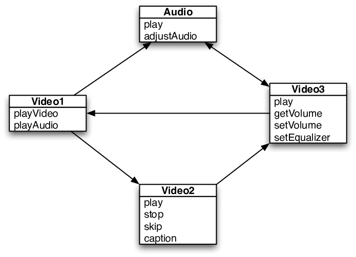
However, different chains of interface adapters result in different lossiness in the interface adaptation, so we need a way to analyze the chaining of lossy interface adapters. We will look at another example in figure 2, where there are four interfaces and six interface adapters, each of the latter represented by an arrow from the source interface to the target interface it converts from and to.

Each interface may have the following characteristics:

•

Video1 can play both video and audio files.
•

Video2 can only play video files, but can stop playback, skip over a fixed amount of time, and select captions.
•

Video3 can only play video files, but can get and set the volume and set the equalizer for the audio output.
•

Audio can only play video files, but can set audio properties, which are the volume and the equalizer.

And each interface adapter may be implemented as in the following, where methods in a target interface not mentioned are not adapted to:

•

The adapter Video1toVideo2, which converts Video1 to Video2, may implement the play method of Video2 by using the playVideo method of Video1.
•

The adapter Video2toVideo3, which converts Video2 to Video3, may implement the play method of Video3 by using the play method of Video2.
•

The adapter Video1toAudio, which converts Video1 to Audio, may implement the play method of Audio by using the playAudio method of Video1.
•

The adapter AudiotoVideo3, which converts Audio to Video3, may implement the setVolume and setEqualizer methods of Video3 by using the adjustAudio method of Audio.²² 2 While it may seem odd to have an adapter from Audio to Video3 which cannot adapt a playback method, it can still be useful when someone wishes to reduce loud noises from an audio device with interface Audio using a remote control that only understands the interface Video3.
•

The adapter Video3toAudio, which converts Video3 to Audio, may implement the adjustAudio method of Audio by using the setVolume and setEqualizer methods of Video3.
•

The adapter Video3toVideo1, which converts Video3 to Video1, may implement the playVideo method of Video1 using the play method of Video3.

A service with interface Video1 may be available, and we may want to access it using a client that only understands interface Video3. There is no interface adapter which directly converts interface Video1 to Video3, but there are interface adapter chains which can indirectly do the conversion. Chaining Video1toVideo2 with Video2toVideo3 or chaining Video1toAudio with AudiotoVideo3 can convert interface Video1 to Video3.

Given multiple possible interface adapter chains, we would want to use the best interface adapter chain that can provide the most methods in the target interface. Associating a cost with an adapter depending on how well it adapts the methods in its target interface and using minimum-cost path algorithms such as Dijkstra’s algorithm [5] would be an obvious approach to choose the best interface adapter chain. However, this naive approach would not work as we will see from the example in figure 2.

Video1toAudio and AudiotoVideo3 can adapt one out of two methods in Audio and Video3, respectively. In contrast, Video1toVideo2 and Video2toVideo3 can adapt one out of four methods in Video2 and Video3. One might think that the Video1toAudio and AudiotoVideo3 chain would be better than the Video1toVideo2 and Video2toVideo3 chain simply by looking at how lossy each interface adapter is, but one would be wrong.

AudiotoVideo3 requires the adjustAudio method in Audio to implement the setVolume and setEqualizer methods in Video3. However, Video1toAudio cannot implement the adjustAudio method in Audio, so the Video1toAudio and AudiotoVideo3 chain ends up with no available methods for Video3. In contrast, the Video1toVideo2 and Video2toVideo3 chain can provide the method play for Video3. A single number for each interface adapter cannot express such dependencies properly, so we need a more precise approach to analyze the lossiness in interface adapter chains.

In the rest of the paper, we will discuss how to mathematically analyze the lossiness incurred from the chaining of interface adapters. We will also assume that interface adapters are implemented as transparently as possible: while an interface adapter may not be able to provide all of the methods in the target interface, the methods it will provide will work just as if they were invoked directly on a service having the target interface.

3 Mathematical basics

We can start formalizing the problem of lossy interface adaptation by defining an interface adapter graph. This is a directed graph where interfaces are nodes and adapters are edges. If there are interfaces $I_{1}$ and $I_{2}$ with an adapter $A$ that adapts source interface $I_{1}$ to target interface $I_{2}$ , then $I_{1}$ and $I_{2}$ would be nodes in the interface adapter graph while $A$ would be a directed edge from $I_{1}$ to $I_{2}$ .

We do not assume that there can be at most one adapter which can adapt one interface to another. This reflects the fact that there can be multiple adapters from different developers, similar to how there can be multiple device drivers available for a graphics card. It also simplifies some of the arguments, although they would still hold even with such a restriction with only minor changes in the proofs.

We will be using a range convention for the index notation used to express matrixes and vectors [4].

3.1 Method dependencies

The next step is to formally describe each adapter, i.e. each edge in the interface adapter graph, in a way that would be useful for analyzing lossiness. We should be able to figure out which methods in the target interface can be provided by an interface adapter given the methods available in the source interface. We do this by defining a method dependency matrix, a boolean matrix which describes how an interface adapter implements methods in the target interface using available methods in the source interface.

The method dependency matrix $a_{ji}$ for an adapter $A$ , where $a_{ji}$ represents either the matrix itself or a single component in the matrix depending on the context, is defined by how the adapter depends on the availability of a method in the source interface in order to implement a method in the target interface. $a_{ji}$ is true if and only if method $j$ in the target interface can be implemented only if method $i$ in the source interface is available. We denote the method dependency matrix associated with an adapter $A$ as $\mathit{depend}(A)$ .

We also define a method availability vector $p_{i}$ for an interface, where each component $p_{i}$ is true if and only if method $i$ is available. This boolean vector is not intrinsic to an interface, unlike the method dependency matrix which is intrinsic to an interface adapter. Instead, it is used to represent the lossiness in interface adaptation such that method $i$ in the target interface can be used only if $p_{i}$ is true. For a fully functional service that implements all methods specified in its interface, the components of its method availability vector should all be true. We denote the number of true components in method availability vector $p_{i}$ as $\|p_{i}\|$ , which is equivalent to the Manhatten norm [19] when true and false components are replaced by 1 and 0, respectively.

Given method availability vector $p_{i}$ for a source interface and the method dependency matrix $a_{ji}$ for an interface adapter, we can derive the method availability vector $q_{j}$ for the target interface. A method $j$ in the target interface can only be implemented if all of the methods it depends on are available in the source interface. So if $q_{j}$ is to be true for fixed $j$ , then all $p_{i}$ must be true when $a_{ji}$ is true:

q_{j}=\bigwedge_{i}(a_{ji}\rightarrow p_{i})=\bigwedge_{i}(\neg a_{ji}\vee p_{i})

(1)

However, equation (1) is incomplete in that it does not properly distinguish between methods which can always be implemented and methods which cannot be implemented given the source interface. For example, a method that returns the value of $\pi$ does not need anything from the source interface, whereas there would be no way to implement a video playback method given only a source interface specialized exclusively for audio playback. For both cases, all $a_{ji}$ are false for a specific method $j$ , and equation (1) would give the wrong result for the latter case.

This can be worked around by defining a dummy method that is never available for every interface. We arbitrarily call this “method 1”, so that $p_{1}$ will always be false for any method availability vector. It is easy to see that extending the definition of the method dependency matrix with the following rules is consistent with our definitions and equations for the method dependency matrix and method availability vector:

•

$a_{11}$ is true, while $a_{1i}$ is set to false for all $i\neq 1$ .
•

If method $j$ can always be implemented in the target interface, set $a_{ji}$ to false for all $i$ .
•

If method $j$ can never be implemented given the source interface, set $a_{j1}$ to true, while $a_{ji}$ is set to false for all $i\neq 1$ .
•

If method $j$ depends on the availability of actual methods in the source interface, then $a_{j1}$ is false.

For succintness, we denote a method availability vector for interface $I$ which represents that all methods are available, i.e. when the component for the dummy method is false while all the other components are true, by $\mathbf{1}^{\prime}_{I}$ .

We also define the operator $\otimes$ for a method dependency matrix as applied to a method availability vector to represent the operation in equation (1), or in other words:

a_{ji}\otimes p_{i}\equiv\bigwedge_{i}(\neg a_{ji}\vee p_{i})

(2)

It is easy to see that a square boolean matrix where the diagonals are true and the rest of the components are false is an identity matrix for the adaptation operator $\otimes$ . We denote an identity matrix with $n$ rows as $\mathbf{I}_{n}$ .

3.2 Adapter composition

To analyze the chaining of lossy interface adapters, we are also interested in how to derive a composite method dependency matrix from the composition of two method dependency matrixes, which would be equivalent to describing the chaining of two interface adapters as if they were a single interface adapter.

Given interfaces $I_{1}$ , $I_{2}$ , and $I_{3}$ , let the corresponding method availability vectors be $p_{i}$ , $q_{j}$ , and $r_{k}$ . In addition, let there be interface adapters $A_{1}$ and $A_{2}$ , where $A_{1}$ converts $I_{1}$ to $I_{2}$ and $A_{2}$ converts $I_{2}$ to $I_{3}$ , with corresponding method dependency matrixes $a_{ji}$ and $b_{kj}$ , respectively. We would like to know how to derive the method dependency matrix that would correspond to an interface adapter equivalent to $A_{1}$ and $A_{2}$ chained together.

From equation (1) and our assumptions:

$\displaystyle r_{k}$	$\displaystyle=$	$\displaystyle\bigwedge_{j}(\neg b_{kj}\vee q_{j})$
	$\displaystyle=$	$\displaystyle\bigwedge_{j}\left(\neg b_{kj}\vee\bigwedge_{i}(\neg a_{ji}\vee p_{i})\right)$
	$\displaystyle=$	$\displaystyle\bigwedge_{j}\bigwedge_{i}(\neg b_{kj}\vee\neg a_{ji}\vee p_{i})$
	$\displaystyle=$	$\displaystyle\bigwedge_{i}\bigwedge_{j}(\neg b_{kj}\vee\neg a_{ji}\vee p_{i})$
	$\displaystyle=$	$\displaystyle\bigwedge_{i}\left(\bigwedge_{j}(\neg b_{kj}\vee\neg a_{ji})\vee p_{i}\right)$
	$\displaystyle=$	$\displaystyle\bigwedge_{i}\left(\neg\bigvee_{j}(b_{kj}\wedge a_{ji})\vee p_{i}\right)$

We reuse the operator $\otimes$ to represent the composition of two method dependency matrixes, and by comparing the above with equation (1), we can define it as:

b_{kj}\otimes a_{ji}=\bigvee_{j}(b_{kj}\wedge a_{ji})

(3)

$\mathbf{I}_{n}$ from section 3.1 is also an identity matrix for the method dependency matrix composition operator $\otimes$ .

The $\otimes$ operator is ‘‘associative’’³³ 3 It is not technically associative in this context as the $\otimes$ operator as applied to method dependency matrixes is not really the same as the $\otimes$ operator as applied to a method dependency matrix and a method availability vector, similarly to how $\times$ for numbers is different from $\times$ for sets. when applied to method dependency matrixes and a method availability vector, i.e. $b_{kj}\otimes(a_{ji}\otimes p_{i})=(b_{kj}\otimes a_{ji})\otimes p_{i}$ , which shows that in terms of lossiness, chaining adapters and then applying it to a source interface is equivalent to applying each adapter one by one to the source interface:

$\displaystyle b_{kj}\otimes(a_{ji}\otimes p_{i})$	$\displaystyle=$	$\displaystyle\bigwedge_{j}\left(\neg b_{kj}\vee\bigwedge_{i}(\neg a_{ji}\vee p_{i})\right)$
	$\displaystyle=$	$\displaystyle\bigwedge_{j}\bigwedge_{i}(\neg b_{kj}\vee\neg a_{ji}\vee p_{i})$
	$\displaystyle=$	$\displaystyle\bigwedge_{i}\bigwedge_{j}(\neg b_{kj}\vee\neg a_{ji}\vee p_{i})$
	$\displaystyle=$	$\displaystyle\bigwedge_{i}\bigwedge_{j}(\neg(b_{kj}\wedge a_{ji})\vee p_{i})$
	$\displaystyle=$	$\displaystyle\bigwedge_{i}\left(\bigwedge_{j}\neg(b_{kj}\wedge a_{ji})\vee p_{i}\right)$
	$\displaystyle=$	$\displaystyle\bigwedge_{i}\left(\neg\bigvee_{j}(b_{kj}\wedge a_{ji})\vee p_{i}\right)$
	$\displaystyle=$	$\displaystyle(b_{kj}\otimes a_{ji})\otimes p_{i}$

Likewise, method dependency matrix composition is associative:

$\displaystyle c_{lk}\otimes(b_{kj}\otimes a_{ji})$	$\displaystyle=$	$\displaystyle\bigvee_{k}\left(c_{lk}\wedge\bigvee_{j}(b_{kj}\wedge a_{ji})\right)$
	$\displaystyle=$	$\displaystyle\bigvee_{k}\bigvee_{j}(c_{lk}\wedge b_{kj}\wedge a_{ji})$
	$\displaystyle=$	$\displaystyle\bigvee_{j}\bigvee_{k}(c_{lk}\wedge b_{kj}\wedge a_{ji})$
	$\displaystyle=$	$\displaystyle\bigvee_{j}\left(\bigvee_{k}(c_{lk}\wedge b_{kj})\wedge a_{ji})\right)$
	$\displaystyle=$	$\displaystyle(c_{lk}\otimes b_{kj})\otimes a_{ji}$

However, method dependency matrix composition is not commutative, as can be easily seen by considering the composition of method dependency matrixes that are not square matrixes.

We can also formalize the somewhat vague intuition that a longer interface adapter chain is worse in terms of lossiness. If $A_{1}$ and $A_{2}$ are interface adapters, where $A_{1}$ converts $I_{1}$ to $I_{2}$ and $A_{2}$ converts $I_{2}$ to $I_{3}$ , with $a_{ji}=\mathit{depend}(A_{1})$ and $b_{kj}=\mathit{depend}(A_{2})$ in which $a_{11}$ and $b_{11}$ are both true as in section 3.1, then for $p_{i}=b_{kj}\otimes\mathbf{1}^{\prime}_{I_{2}}$ and $p^{\prime}_{i}=b_{kj}\otimes a_{ji}\otimes\mathbf{1}^{\prime}_{I_{1}}$ :

p_{k}=(\neg b_{k1}\vee f)\wedge\bigwedge_{j\neq 1}(\neg b_{kj}\vee t)=\neg b_{k1}

$\displaystyle p^{\prime}_{k}$	$\displaystyle=$	$\displaystyle\bigwedge_{j}\left(\neg b_{kj}\vee\left((\neg a_{j1}\vee f)\wedge\bigwedge_{i\neq 1}(\neg a_{ji}\vee t)\right)\right)$
	$\displaystyle=$	$\displaystyle\bigwedge_{j}(\neg b_{kj}\vee\neg a_{j1})$
	$\displaystyle=$	$\displaystyle\neg b_{k1}\wedge\bigwedge_{j\neq 1}(\neg b_{kj}\vee a_{j1})$

\therefore p^{\prime}_{k}\rightarrow p_{k}

(4)

With $I_{1}$ and $I_{2}$ being the source interfaces for the interface adapters that $a_{ji}$ and $b_{kj}$ represent, respectively, we can also infer from equation (4) that

\|b_{kj}\otimes\mathbf{1}^{\prime}_{I_{2}}\|\geq\|b_{kj}\otimes a_{ji}\otimes\mathbf{1}^{\prime}_{I_{1}}\|

(5)

which, along with the associativity of method dependency matrix composition, formalizes the notion that extending an interface adapter chain is worse in terms of lossiness.

The definitions of the method dependency matrix and the method availability vector in section 3.1, along with the associativity rules proven in this section, provide a succinct way to mathematically express and analyze the chaining of lossy interface adapters.

3.3 An example

As an example, we apply the mathematical framework to the interfaces and adapters in figure 2. We will denote interfaces Video1, Video2, Video3, and Audio as $I_{1}$ , $I_{2}$ , $I_{3}$ , and $I_{4}$ , respectively, while $A_{1}$ , $A_{2}$ , $A_{3}$ , $A_{4}$ , $A_{5}$ , and $A_{6}$ denote the interface adapters Video1toVideo2, Video2toVideo3, Video1toAudio, AudiotoVideo3, Video3toAudio, and Video3toVideo1, respectively. We also index each method in the order they appear in figure 2 along with an extra dummy method with index 1, and let $a^{k}_{ji}=\mathit{depend}(A_{k})$ . Figure 2 is already an interface adapter graph, which is simplified and labeled in figure 3.

Some method dependency matrixes would be:

a^{1}_{ji}=\left(\begin{array}[]{ccc}t&f&f\\ f&t&f\\ t&f&f\\ t&f&f\\ t&f&f\end{array}\right)

a^{2}_{ji}=\left(\begin{array}[]{ccccc}t&f&f&f&f\\ f&t&f&f&f\\ t&f&f&f&f\\ t&f&f&f&f\\ t&f&f&f&f\end{array}\right)

a^{5}_{ji}=\left(\begin{array}[]{ccccc}t&f&f&f&f\\ t&f&f&f&f\\ f&f&f&t&t\end{array}\right)

Given a fully functional service which conforms to interface Video1, we would expect that only the play method would be available for interface Video3 after going through the adapter chain $A_{1}$ and $A_{2}$ , which can be verified by computing the method availability vector $a^{2}_{kj}\otimes a^{1}_{ji}\otimes\mathbf{1}^{\prime}_{I_{1}}$ :

a^{2}_{kj}\otimes a^{1}_{ji}\otimes\mathbf{1}^{\prime}_{I_{1}}=[f,t,f,f,f]

One can also verify the following by hand, which would be expected from the associativity of $\otimes$ . Associativity can be very useful in developing algorithms analyzing chains of lossy interface adapters, since fragments of an interface adapter chain can be assembled independently and still give the same method dependency matrix for the whole chain.

$\displaystyle a^{5}_{lk}\otimes a^{2}_{kj}\otimes a^{1}_{ji}\otimes\mathbf{1}^{\prime}_{I_{1}}$
	$\displaystyle=$	$\displaystyle a^{5}_{lk}\otimes(a^{2}_{kj}\otimes(a^{1}_{ji}\otimes\mathbf{1}^{\prime}_{I_{1}}))$
	$\displaystyle=$	$\displaystyle((a^{5}_{lk}\otimes a^{2}_{kj})\otimes a^{1}_{ji})\otimes\mathbf{1}^{\prime}_{I_{1}}$
	$\displaystyle=$	$\displaystyle(a^{5}_{lk}\otimes a^{2}_{kj})\otimes(a^{1}_{ji}\otimes\mathbf{1}^{\prime}_{I_{1}})$
	$\displaystyle=$	$\displaystyle[f,f,f]$

We can also verify the following, which is consistent with equations (4) and (5), and is in line with the intuition that extending an adapter chain can only be worse in terms of lossiness, although this does not mean that a longer adapter chain is always worse than a shorter adapter chain.

	$\displaystyle a^{5}_{lk}\otimes\mathbf{1}^{\prime}_{I_{3}}$	$\displaystyle=$	$\displaystyle[f,f,t]$
	$\displaystyle a^{5}_{lk}\otimes a^{2}_{kj}\otimes\mathbf{1}^{\prime}_{I_{2}}$	$\displaystyle=$	$\displaystyle[f,f,f]$

4 Optimal adapter chaining

One of the things that could be hoped from the mathematical framework in section 3 is that it could help with the development of an efficient algorithm for optaining an optimal interface adapter chain from an actual service to a target interface that incurs the least loss in terms of functionality. Unfortunately, the problem is NP-complete, as will be shown in this section, dashing hopes for such an algorithm.

First, we must formally describe the problem, which we will call CHAIN. Let us have an interface adapter graph $(\{I_{i}\},\{A_{i}\})$ , where $\{I_{i}\}$ is the set of interfaces and $\{A_{i}\}$ is the set of interface adapters. Let $a^{k}$ be the method dependency matrix associated with adapter $A_{k}$ . Let $S\in\{I_{i}\}$ be the source interface and $T\in\{I_{i}\}$ be the target interface. Then the problem is whether there is an interface adapter chain $[A_{P(1)},A_{P(2)},\ldots,A_{P(m)}]$ such that the source of $A_{P(1)}$ is $S$ , the target of $A_{P(m)}$ is $T$ , and $\|v^{T}\|=\|a^{P(m)}\otimes\cdots\otimes a^{P(2)}\otimes a^{P(1)}\otimes\mathbf{1}^{\prime}_{S}\|$ is at least as large as some parameter $N$ .

Informally, this is an optimization problem which tries to maximize the number of methods that can be used in a fixed target interface, obtained by applying an interface adapter chain on a fully-functional service which conforms to the source interface. We show that the problem is NP-complete by reducing 3SAT [3] to CHAIN.

Based on the conjunctive normal form of a boolean expression $E$ with exactly 3 literals in each clause, we will construct an interface adapter graph $G$ in three parts and the corresponding method dependency matrixes. One part will model the setting of each variable to true or false, another part will model the value of each clause once the variable values are set, and the last part will serve as a filter so that $E$ is satisfiable if and only if there is a chain in $G$ such that $\|v^{T}\|$ equals the number of clauses in $E$ .

Figure 4 shows what a reduction from an instance of 3SAT to an instance of CHAIN would generally look like.

4.1 Representing values

We will represent values of literals and clauses using the method availability vector for each interface, where all but one of the nodes in the constructed interface adapter graph will contain the same set of methods. At certain points in the interface adapter graph, a true or false component in the method availability vector would directly map to the value of a literal or a clause.

For almost all nodes, including the source, the set of methods will be fixed with one dummy method, one method for each clause, and one method for each literal, so almost all method dependency matrixes will be square matrixes. As the method dependency matrixes will have large parts in common with the identity matrix, we will only be mentioning how each matrix differs from the identity matrix.

Each method will be labeled as follows:

•

The dummy method will be labeled $d$ .
•

For each clause $c_{i}$ , the method will be labeled $c_{i}$ .
•

For each variable $v_{i}$ , the method for the variable itself will be labeled $l_{i}$ , while the method for the negation of the variable will be labeled $\overline{l_{i}}$ .

There is a single method dependency matrix used in the filter part of the graph that will not be a square matrix.

4.2 Handling literals

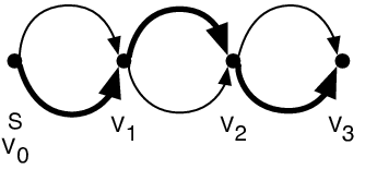
The basic approach of this part of the graph, which we will call the variable handling subgraph, is to set the value for each variable depending on which adapters are chosen to be included in the chain. For each variable $v_{1}$ , $v_{2}$ , …, $v_{v}$ , we define nodes $V_{1}$ , $V_{2}$ , …, $V_{v}$ , and we let $V_{0}=S$ . Between each $V_{i-1}$ and $V_{i}$ , we define two adapters which will leave everything about the method availability vector unchanged from one node to the next except for the components corresponding to the literals for $v_{i}$ . One will make the variable effectively true, while the other will make the variable effectively false.

For each $V_{i}$ for $i>0$ , we will define a positive literal adapter $A_{l_{i}}$ with method dependency matrix $a^{l_{i}}$ and a negative literal adapter $A_{\overline{l_{i}}}$ with method dependency matrix $a^{\overline{l_{i}}}$ . For the positive literal adapter, $a^{l_{i}}_{l_{i}j}$ is false for all $j$ , $a^{l_{i}}_{\overline{l_{i}}d}$ is true, and $a^{l_{i}}_{\overline{l_{i}}j}$ is false for all $j$ other than $d$ . Similarly for the negative literal adapter, $a^{\overline{l_{i}}}_{\overline{l_{i}}j}$ is false for all $j$ , $a^{\overline{l_{i}}}_{l_{i}d}$ is true, and $a^{\overline{l_{i}}}_{l_{i}j}$ is false for all $j$ other than $d$ .

It should then be easy to see that for a method availability vector $p_{i}$ with a false $p_{d}$ , all components of $a^{l_{i}}\otimes p_{i}$ should be the same as $p_{i}$ except for the components corresponding to $l_{i}$ and $\overline{l_{i}}$ , which will be true and false, respectively. Likewise, all components of $a^{\overline{l_{i}}}\otimes p_{i}$ should be the same as $p_{i}$ except for the components corresponding to $l_{i}$ and $\overline{l_{i}}$ , which will be false and true, respectively.

The rest of the interface adapter graph will be the descendant of $V_{v}$ , so any adapter chain from $S$ to $T$ must go through all of $V_{0}$ , $V_{1}$ , …, $V_{v}$ in order, and for every variable one and only one of the positive literal adapter or the negative literal adapter must be chosen as in figure 5 due to the structure of the variable handling subgraph. This is equivalent to choosing a variable assignment, and at $V_{v}$ , the method availability vector $p_{i}$ will be such that for each variable $v_{i}$ , $p_{l_{i}}$ and $p_{\overline{l_{i}}}$ will have opposite values, so that it would be the same as setting the value of $v_{i}$ to $p_{l_{i}}$ .

4.3 Handling clauses

Based on the variable assignment that is taken care of by the variable handling subgraph in section 4.2, this part of the graph, which we will call the clause handling subgraph, is responsible for determining the value of each clause.

In order to model disjunction, not only do we define a node $C_{i}$ for each clause $c_{i}$ , we also define three subnodes $C_{ij}$ , for $j$ from 1 to 3, for each of the literals in the clause. These nodes are separate from those defined in section 4.2. The idea is that if any of the literals are true, then at least one of the nodes will end up with a method availability vector marking the clause as true, so we can use this to mark the same for $C_{i}$ itself. We also set $C_{0}=V_{v}$ for convenience of notation, and $c$ will be the number of clauses.

For each clause $c_{i}$ , there are edges from $C_{i-1}$ to each of the subnodes $C_{ij}$ , and in turn there are edges from each subnode $C_{ij}$ to $C_{i}$ . So there will be three alternate paths from $C_{i-1}$ to $C_{i}$ .

For edge $(C_{i-1},C_{ij})$ , if $l$ corresponds to the literal for $C_{ij}$ , the method dependency matrix $a$ for the edge is defined by setting $a_{c_{i}l}$ to true and $a_{c_{i}k}$ to false for all $k$ other than $l$ . Then it should be easy to see that $a\otimes p$ is the same as the method availability vector $p$ except for the component $p_{c_{i}}$ , which would be true if and only if $p_{l}$ is also true. For edge $(C_{ij},C_{i})$ , the corresponding method dependency matrix is simply the identity matrix.

If clause $c_{i}$ is true, then one of the literals must be true. Then the path through the subnode $C_{ij}$ for the true literal will result in a true component for the clause in the method availability vector at $C_{i}$ . If the clause is not true, then the same component will be false no matter the path taken, since it will be false for all subnodes $C_{ij}$ .

$T$ will be the descendant of $C_{c}$ , and since the source is in the variable handling subgraph, which is only connected to the clause handling subgraph by $C_{0}$ , any interface adapter chain from $S$ to $T$ must go through each of the nodes $C_{0}$ , $C_{1}$ , …, $C_{c}$ in order as in figure 6. And if all clauses are true with the variable assignment done in the variable handling subgraph, which is equivalent to choosing which adapters to include from the subgraph, only then will there be a path from $C_{0}$ to $C_{c}$ which will result in true components for all clauses in the method availability vector at $C_{c}$ .

4.4 Filtering

The last part of the constructed interface adapter graph is the filtering part, which discards all methods corresponding to literals from the method availability vector so that only the dummy method and methods corresponding to clauses remain.

The filtering subgraph is made up of only two nodes and a single edge. One of the nodes is the target $T$ , and its interface only contains the dummy method and all the methods corresponding to clauses. The other node is $C_{c}$ from section 4.3. The $(c+1)\times(2v+c+1)$ method dependency matrix $a_{ji}$ for the edge from $C_{c}$ to $T$ defined as follows accomplishes the filtering:

•

For all clauses $c_{i}$ , $a_{c_{i}c_{i}}$ is true.
•

For the dummy method, $a_{dd}$ is true.
•

All other compenents are false.

4.5 Analysis of the reduction

The constructed interface adapter graph has $v+4c+2$ nodes and $2v+6c+1$ edges, where $v$ is the number of variables and $c$ is the number of clauses. Also, each method dependency matrix has at most $(1+c+2v)^{2}$ components, so the reduction of a candidate for 3SAT to a candidate for CHAIN can be done in polynomial time. So we just need to verify that there is a positive answer for CHAIN with $N=c$ if and only if there is a positive answer for 3SAT.

If the boolean expression is satisfiable, then there is a variable assignment that makes it true. Consider the following interface adapter chain. In the variable handling subgraph, include edges that correspond to the variable assignment. In the clause handling subgraph, there is guaranteed to be a path where all components corresponding to clauses in the method availability vector at the target end up being true, given the path in the variable handling subgraph, so use this path in the chain. Then $\|v^{T}\|$ will be exactly $c$ .

Conversely, suppose there is an adapter chain such that $\|v^{T}\|=c$ . Then assigning values to variables according to the path through the variable handling subgraph results in a satisfying variable assignment for the boolean expression. This is because the clause handling subgraph and the fact that $\|v^{T}\|=c$ together imply that all clauses are true for the derived variable assignment. And given an arbitrary interface adapter chain and an optimal chain, it is easy to verify whether the arbitrary adapter chain is not optimal, so CHAIN is NP-complete.

5 A greedy algorithm

As shown in section 4, the problem of finding an optimal interface adapter chain that would make available the most methods in the target interface is an NP-complete problem. Short of developing a polynomial-time algorithm for an NP-complete problem, practical systems will have to use a heuristic algorithm or an exponential-time algorithm with reasonable performance in practice.

Algorithm 1 is a greedy algorithm that finds an optimal interface adapter chain between a given source interface and a target interface. Given an interface adapter graph $G$ , it works by looking at every possible acyclic adapter chain with an arbitrary source that results in the target interface $t$ in order of increasing loss, taking advantage of equation (5), until we find a chain that starts with the desired source interface $s$ . In this context, loss means the number of methods unavailable in the target interface given a fully functional service with the source interface, which is computed in algorithm 2, so the algorithm is guaranteed to find the optimal interface adapter chain. In the worst case, however, the algorithm takes exponential time since there can be an exponential number of acyclic chains in an interface adapter graph.

Algorithm 1 A greedy algorithm for interface adapter chaining.

procedure Greedy-Chain(

G=(V,E)

s

t

)

\mathit{C}\leftarrow\{[]\}

\triangleright

chains to extend

\mathit{M}=\emptyset

\triangleright

discarded chains

D\leftarrow\{[]\mapsto\mathbf{I}_{\dim(\mathbf{1}^{\prime}_{t})}\}

\triangleright

method dependency matrixes

while

C\neq\emptyset

c\leftarrow\mbox{element of $C$ minimizing $\textsc{Loss}(c,D)$}

c\neq[]\wedge\mathit{source}(c[1])=s

then

return

c

else if no acyclic chain not in

C\cup M

extends

c

then

C\leftarrow C-\{c\}

M\leftarrow M\cup\{c\}

else

c=[]

then

B\leftarrow\{[e]\,|\,e\in E,\mathit{target}(e)=t\}

else

B\leftarrow\{e:c\,|\,e\in E,\mathit{target}(e)=\mathit{source}(c[1])\}

end if

remove cyclic chains from

B

C\leftarrow C\cup B

D\leftarrow D\cup\{e:c\mapsto D[c]\otimes\mathit{depend}(e)\,|\,e:c\in B\}

end if

end while

end procedure

Algorithm 2 Computing the lossiness of an interface adapter chain.

function Loss(

c

D

)

s\leftarrow\mathit{source}(c[1])

t\leftarrow\mathit{target}(c[|c|])

return

\dim(\mathbf{1}^{\prime}_{t})-\|D[c]\otimes\mathbf{1}^{\prime}_{s}\|

end function

While algorithm 1 may take exponential time in the worst case, results with a similar algorithm from [11] based on a small randomly generated interface adapter graph suggest that the greedy algorithm has acceptable performance in practice.

Algorithm 1 can easily be extended to support the selection of an optimal source interface with weights associated with methods expressing their importance as in algorithm 3. This can be done by checking that the starting point of an interface adapter chain is included in a set of possible source interfaces, instead of just comparing it to a single source interface, and summing the weights for the available methods in the target interface as in algorithm 4 and using equation (4), instead of just counting the methods.

Algorithm 3 Greedy discovery for weighted interface adapter chaining.

procedure Greedy-Chain(

G=(V,E)

S

t

W

)

\mathit{C}\leftarrow\{[]\}

\triangleright

chains to extend

\mathit{M}=\emptyset

\triangleright

discarded chains

D\leftarrow\{[]\mapsto\mathbf{I}_{\dim(\mathbf{1}^{\prime}_{t})}\}

\triangleright

method dependency matrixes

while

C\neq\emptyset

c\leftarrow\mbox{element of $C$ maximizing $\textsc{Weight}(c,D,W)$}

c\neq[]\wedge\mathit{source}(c[1])\in S

then

return

(\mathit{source}(c[1]),c)

else if no acyclic chain not in

C\cup M

extends

c

then

C\leftarrow C-\{c\}

M\leftarrow M\cup\{c\}

else

c=[]

then

B\leftarrow\{[e]\,|\,e\in E,\mathit{target}(e)=t\}

else

B\leftarrow\{e:c\,|\,e\in E,\mathit{target}(e)=\mathit{source}(c[1])\}

end if

remove cyclic chains from

B

C\leftarrow C\cup B

D\leftarrow D\cup\{e:c\mapsto D[c]\otimes\mathit{depend}(e)\,|\,e:c\in B\}

end if

end while

end procedure

Algorithm 4 Computing the weight of an interface adapter chain.

function Weight(

c

D

W=w_{i}

)

s\leftarrow\mathit{source}(c[1])

t\leftarrow\mathit{target}(c[|c|])

p_{i}\leftarrow D[c]\otimes\mathbf{1}^{\prime}_{s}

return

\sum_{p_{i}}w_{i}

end function

Unlike algorithm 1, which would find an interface adapter chain after a single service was presumably found by a service discovery process, algorithm 3 can be used in the service discovery process itself to search for the best service, not just in terms of what is required from the service, but also considering how well the client could use the service. And by weighting the methods in the target interface, it can take into account the importance of each method. By having sufficiently large weights for essential methods compared to those of non-essential methods, algorithm 3 can also guarantee that an adapter chain which makes all essential methods available will always be preferred over those which do not.

6 Related work

The mathematics in this paper was motivated by the interface adapter framework [11] used by the Active Surroundings middleware for ubiquitous computing environments [12]. In order to support a transparent computing experience despite a user moving around locations where similar services may have different interfaces, the framework uses interface adapters to adapt interfaces. [11] defines the problem informally and shows the effectiveness of a greedy algorithm based on uniform cost search [16].

Other work have also used interface adapters to resolve service interface mismatches. Some attempt to aid developers create interface adapters using template-based approaches [1, 14] or mapping specifications [21]. Others reduce the number of required interface adapters by chaining them together [15], while others use a chain of interface adapters to provide backwards compatibility as interfaces evolve [9, 10]. These chaining approaches ignore that one chain may be worse than others in terms of lossiness.

Analyzing the chaining of lossy interface adapters is in many ways similar to depedency analysis in software architecture [6, 13, 8, 18]. These are designed to support maintenance of large software systems and usually consider a lossy connection between software components to be the exception and not the norm. Techniques used in software architecture such as code analysis [17] or fault injection [2] could also be the basis for deriving the method dependency matrixes for interface adapters.

7 Conclusions

By chaining a series of interface adapters, it is possible for a single-interface client use a much wider variety of services with heterogeneous interfaces without requiring an explosive number of interface adapters. However, as an interface adapter may not be able to convert one interface to another perfectly, we have developed a mathematical framework which can be used to analyze the lossiness incurred during chained interface adaptation.

The mathematical framework defines the method dependency matrix, the method availability vector, and the composition operation for describing the properties of composed adapters, which was also proved to be associative. The framework could be used to analyze the lossiness in interface adapter chains and develop algorithms for finding such chains.

However, finding an optimal interface adapter chain is an NP-complete problem, which can be proven by reducing 3SAT to CHAIN. A greedy algorithm for finding an optimal interface adapter chain requiring exponential time in the worst case was suggested.

This paper has only considered the all-or-nothing case where a method in a target interface can be completely implemented using methods in the source interface. However, in certain cases the method could only be implemented partially. One possible extension to the mathematical framework is to consider partial adaptation of such methods. Extending it so that it can analyze the lossiness when services are composed is another possibility. Heuristic algorithms with provable approximation bounds is another topic that would be worth looking into in the future.

References

[1] Boualem Benatallah, Fabio Casati, Daniela Grigori, Hamid R. Motahari Nezhad, and Farouk Toumani. Developing adapters for web services integration. In Proceedings of the 17th International Conference on Advanced Information Systems Engineering, volume 3520 of Lecture Notes in Computer Science, pages 415–429, Porto, Portugal, June 2005. Springer-Verlag.
[2] A. Brown, G. Kar, and A. Keller. An active approach to characterizing dynamic dependencies for problem determination in a distributed environment. In Proceedings of the 2001 IEEE/IFIP International Symposium on Integrated Network Management, pages 377–390, May 2001.
[3] Stephen A. Cook. The complexity of theorem-proving procedures. In Proceedings of the Third Annual ACM Symposium on Theory of Computing, pages 151–158. ACM Press, 1971.
[4] M. Crampin and F. A. E. Pirani. Applicable Differential Geometry, chapter 0, pages 5–7. Number 59 in London Mathematical Society Lecture Note Series. Cambridge University Press, March 1987.
[5] E. W. Dijkstra. A note on two problems in connexion with graphs. Numerische Mathematik, 1:269–271, June 1959.
[6] Stuart I. Feldman. Make –– a program for maintaining computer programs. Software Practice and Experience, 9(4):255–265, April 1979.
[7] Erich Gamma, Richard Helm, Ralph Johnson, and John M. Vlissides. Design Patterns: Elements of Reusable Object-Oriented Software. Addison-Wesley, November 1994.
[8] J. Gao, G. Kar, and P. Kemarii. Approaches to building self healing systems using dependency analysis. In Proceedings of the 2004 IEEE/IFIP Network Operations and Management Symposium, volume 1, pages 119–132, April 2004.
[9] Sven Moritz Hallberg. Eternal compatibility in theory. The Monad.Reader, 2, May 2005.
[10] Piotr Kaminski, Marin Litoiu, and Hausi Müller. A design technique for evolving web services. In Proceedings of the 2006 Conference of the Center for Advanced Studies on Collaborative Research, Toronto, Ontario, Canada, October 2006. ACM Press.
[11] Byoungoh Kim, Kyungmin Lee, and Dongman Lee. An adapter chaining scheme for service continuity in ubiquitous environments with adapter evaluation. In Proceedings of the Sixth IEEE International Conference on Pervasive Computing and Communications, pages 537–542. IEEE Computer Society Press, March 2008.
[12] Dongman Lee, Seunghyun Han, Insuk Park, Saehoon Kang, Kyungmin Lee, Soon J. Hyun, Young-Hee Lee, and Geehyuk Lee. A group-aware middleware for ubiquitous computing environments. In Proceedings of the 14th International Conference on Artificial Reality and Telexistence, pages 291–298, December 2004.
[13] Joseph P. Loyal and Susan A. Mathisen. Using dependence analysis to support the software maintenance process. In Proceedings of the 1993 Conference on Software Maintenance, pages 282–291, September 1997.
[14] Hamid Reza Motahari Nezhad, Boualem Benatallah, Axel Martens, Francisco Curbera, and Fabio Casati. Semi-automated adaptation of service interactions. In Proceedings of the 16th International Conference on World Wide Web, pages 993–1002, 2007.
[15] Shankar R. Ponnekanti and Armando Fox. Application-service interoperation without standardized service interfaces. In Proceedings of the First IEEE International Conference on Pervasive Computing and Communications, 2003.
[16] Stuart Russell and Peter Norvig. Artificial Intelligence: A Modern Approach, chapter 3, page 75. Prentice-Hall, 2nd edition, 2003.
[17] Barbara G. Ryder. Constructing the call graph of a program. IEEE Transactions on Software Engineering, 5(3):216–226, May 1979.
[18] Neeraj Sangal, Ev Jordan, Vineet Sinha, and Daniel Jackson. Using dependency models to manage complex software architecture. In Proceedings of the 2005 ACM SIGPLAN Conference on Object-Oriented Programming Systems, Languages & Applications, pages 167–176. ACM Press, 2005.
[19] Gilbert W. Stewart. Matrix Algorithms: Basic Decompositions, chapter 1, page 46. Society for Industrial and Applied Mathematics, 1998.
[20] W3C. Soap version 1.2. http://www.w3.org/TR/soap12, April 2007.
[21] Johannes Maria Zaha, Marco Geisenberger, and Martin Groth. Compatibility test and adapter generation for interfaces of software components. In Distributed Computing and Internet Technology, volume 3347 of Lecture Notes in Computer Science, pages 318–328. Springer-Verlag, November 2004.

A Mathematical Basis for the Chaining of Lossy Interface Adapters

Abstract

1 Introduction

2 Interface adaptation

3 Mathematical basics

3.1 Method dependencies

3.2 Adapter composition

3.3 An example

4 Optimal adapter chaining

4.1 Representing values

4.2 Handling literals

4.3 Handling clauses

4.4 Filtering

4.5 Analysis of the reduction

5 A greedy algorithm

6 Related work

7 Conclusions

References

A Mathematical Basis for
the Chaining of Lossy Interface Adapters