Quasi-long-range order in the 2D XY model with random phase shifts
Abstract
We study the square-lattice XY model in the presence of random phase shifts. We consider two different disorder distributions with zero average shift and investigate the low-temperature quasi-long-range order phase which occurs for sufficiently low disorder. By means of Monte Carlo simulations we determine several universal quantities which are then compared with the analytic predictions of the random spin-wave theory. We observe a very good agreement which indicates that the universal long-distance behavior in the whole low-disorder low-temperature phase is fully described by the random spin-wave theory.
1 Introduction
The two-dimensional XY model with random phase shifts (RPXY) describes the thermodynamic behavior of several disordered systems, such as magnetic systems with random Dzyaloshinskii-Moriya interactions [1], Josephson junction arrays with geometrical disorder [2, 3], crystal systems on disordered substrates [4], and vortex glasses [5]. See [6, 7] for recent reviews. The RPXY model is defined by the Hamiltonian
| (1) |
where , , and the sum runs over the bonds of a square lattice. The phases are uncorrelated quenched random variables with zero average. A Gaussian distribution,
| (2) |
has been considered in most of the studies of the RPXY. We denote the RPXY with Gaussian-distributed phases by GRPXY. The pure XY model is recovered in the limit , while the so-called gauge glass model [8] with uniformly distributed phase shifts is obtained in the limit .
The pure XY model shows a high-temperature paramagnetic phase and a low-temperature phase characterized by quasi-long-range order (QLRO) controlled by a line of Gaussian fixed points. In the latter phase, the spin-spin correlation function decays as for large , with depending on ; for small values of . The two phases are separated by a Kosterlitz-Thouless (KT) transition [9] at [10] . For the correlation length diverges exponentially as and the magnetic susceptibility behaves as , corresponding to .

In this paper we shall discuss the low-temperature behavior of RPXY models for small disorder. It has already been investigated in several works, most of them focussing on the GRPXY; see, e.g., [1, 8, 2, 11, 12, 3, 13, 14, 15, 5, 16, 17, 18, 19, 20, 21, 22, 23, 4, 24, 25, 26, 27, 28, 29, 30, 31, 32, 33, 34, 35, 36, 38, 39, 40, 41, 42, 43, 44, 45, 46]. The expected - phase diagram, which is sketched in Fig. 1, presents two phases at finite temperature: a paramagnetic and a QLRO phase. The paramagnetic phase is separated from the QLRO phase by a transition line, which starts from the pure XY point (denoted by in Fig. 1) at and ends at a zero-temperature disorder-induced transition denoted by at . Note that QLRO is observed only up to a maximum value of the disorder parameter, which is related to the point , where the tangent to the transition line is parallel to the axis. The transition line from to is believed to run (almost) parallel to the axis, with ; see, e.g., [6]. 11 1 The first renormalization-group (RG) analyses based on a Coulomb-gas representation of the models [1] predicted reentrant transitions for any value of , so that . It was then clarified that this was an artefact of the approximations. Indeed, in agrement with the experimental findings [11], numerical works [11, 12, 13, 30] and more careful RG analyses [19, 24, 28, 29, 31, 35] showed the absence of reentrant transitions for sufficiently small values of , that is predicted . For the CRPXY, [19] suggested that the transition line is parallel to the axis below the Nishimori point . It is not clear whether this conjecture is correct. Indeed, the analogous conjecture fails in the case of the 2D Ising model; see [47] and references therein.
The QLRO phase of the pure XY model is expected to survive for sufficiently small values of (see, however, [38] for a recent critical discussion of this scenario). It disappears for large disorder, for [1] . The RPXY model for large disorder, and in particular the gauge-glass model (), has been much investigated [5, 8, 14, 15, 16, 17, 18, 20, 22, 23, 26, 27, 32, 33, 34, 36, 37, 39, 40, 42, 43, 44, 45, 46]. No long-range glassy order can exist at finite temperature [22, 23]. Some numerical works support a zero-temperature transition; see, e.g., [45, 43, 42].
Beside the GRPXY, we also consider a RPXY model with a slightly different distribution, given by
| (3) |
We denote the RPXY model with the distribution (3) by CRPXY. The CRPXY is interesting because it allows to obtain exact results along the so-called Nishimori (N) line [19]
| (4) |
exploiting gauge invariance [48, 19, 49]. For example, the energy density is exactly known along the N line: , where and are the modified Bessel functions. Another important feature of the CRPXY is that along the line the spin-spin and overlap correlation functions are equal,
| (5) |
where the angular and square brackets indicate the thermal average and the quenched average over disorder, respectively. The phase diagram is expected to be analogous to that of GRPXY model. As already noted in [49], the N line must play an important role in the phase diagram, because it is expected to mark the crossover between the region dominated by magnetic correlations and that dominated by randomness. In [19] it was proven that the critical value of along the N line is an upper bound for the values of where magnetic QLRO can exist (note that this does not exclude the existence of a glassy QLRO for ). Therefore, we can identify it as the point where in Fig. 1. The critical value at must satisfy , leaving open the possibility of reentrant transitions.
In this paper we focus on the QLRO phase of RPXY models, and investigate its nature. In particular, we check the random-spin-wave scenario [1], in which the long-distance behavior is essentially identical to that in the model obtained by replacing
| (6) |
in the Hamiltonian (1). We numerically check this scenario by perfoming Monte Carlo (MC) simulations of the GRPXY and CRPXY models and provide conclusive evidence of the existence of a low- phase with QLRO determined by the random spin-wave theory. Some numerical evidence of QLRO in the GRPXY model was already presented in [30].
The paper is organized as follows. In Sec. 2 we summarize the main predictions of the spin-wave theory, which are then compared with the numerical data in Sec. 3. Our conclusions are presented in Sec. 4. The definitions of the quantities we consider are reported in A. In B we report the spin-wave calculation of in the CRPXY model.
2 The random spin-wave theory
In the spin-wave limit the partition function is given by
| (7) |
where the link-variables are uncorrelated quenched random variables with Gaussian probability . For the GRPXY the spin and the overlap correlation functions are given by [1, 49]
| (8) | |||
| (9) |
where is the (infrared-regularized) two-point function of the Gaussian model without disorder
| (10) |
For the CRPXY one should take into account the nontrivial dependence of on . For the overlap correlation function one still obtains (9): for any probability distribution does not depend on randomness in the spin-wave approximation. For the spin correlation function the dependence at is more complex. For we obtain
| (11) |
disregarding terms of order . The derivation is reported in B.
The above-reported results allow us to evaluate the exponents and which are related to the large-distance behavior of the spin and overlap correlation functions:
| (12) | |||
| (13) |
We can thus write for both models, at this level of approximation,
| (14) |
Note that the disorder dependence is completely included in the exponents and . Using these expressions we can campute the universal functions and , which express the ratios and in terms of the corresponding exponents and . It is clear that and are identical [] and disorder independent, hence they coincide with those relevant for the pure XY model. These functions are shown in Fig. 2. Below we show numerically that these predictions are satisfied by our numerical data. This provides a clear evidence for the spin-wave nature of the QLRO in the RPXY models. A similar strategy was applied in [50] to clarify the nature of the low-temperature phase of fully frustrated XY models.


3 Monte Carlo results
In this section we numerically investigate the nature of the QLRO phase that occurs for sufficiently small disorder. In particular, we want to provide a stringent check of the random spin-wave scenario. The quantities which we compure are defined in A.
3.1 Numerical details
We performed MC simulations of the GRPXY and CRPXY models, considering square lattices of linear size with periodic boundary conditions. We set in both cases , which is well below the maximum value ( in the CPRXY model [51] and in the GRPXY model) and considered several values of below the critical temperature , which marks the end of the QLRO phase. MC simulations in the high-temperature phase [51] indicate for the GRPXY and for the CRPXY.
In the simulations we used a mixture of standard Metropolis and overrelaxed microcanonical updates: A single MC step consisted of five microcanonical sweeps followed by one Metropolis sweep. In the MC simulations of the CRPXY model we also used the parallel-tempering method [52, 53]. It allowed us to perform efficient simulations in the region . In the parallel-tempering simulations we considered systems at the same value of and at different inverse temperatures , …, . The largest value corresponded to the minimum temperature value we were interested in. The value was chosen in the paramagnetic phase and was such that thermalization at was sufficiently fast. The intermediate values were chosen such that the acceptance probability of the temperature exchange was at least 5%. Morever, we always included the value , which lies along the N line. This provided a check of the numerical programs, since the MC results could be compared with the known exact results [49]. The overlap correlation functions and corresponding and were obtained by simulating two independent replicas for each disorder sample.
In the case of the GRPXY model we performed standard MC simulations at , for lattice sizes . Typically, we considered 50000 disorder realizations and performed MC steps for each of them. In the case of the CRPXY model the parallel-tempering method allowed us to investigate the temperature range down to , which is below the N line, i.e. satisfies . We performed simulations for lattice sizes . Typically, we considered 25000 disorder realizations. For we also performed standard MC runs up to .
3.2 QLRO in RPXY models


We estimate the exponents and by studying the finite-size behavior of the susceptibilities and defined in A. Indeed, for they behave as
| (15) |
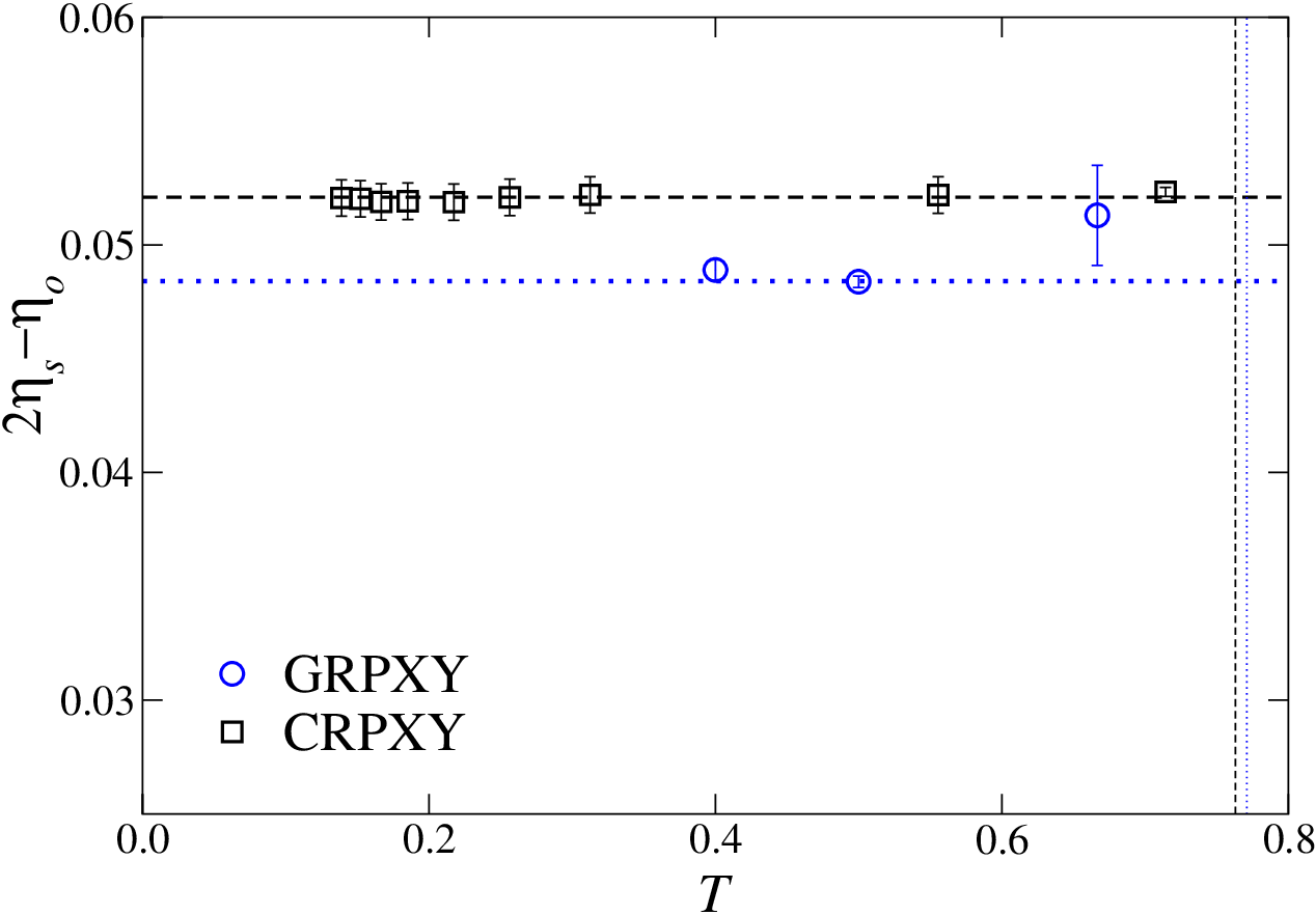
Estimates of are shown in Fig. 3. On a logarithmic scale, the data fall on a straight line, indicating that the asymptotic behavior (15) already holds for the values of we consider. In Fig. 4 we show the estimates of and for the GRPXY and CRPXY model. For they agree with the spin-wave approximations (12) and (13). Morever, they appear to be mostly independent of the model, in agreement with the random spin-wave predictions (note that for ). For a more quantitative check, in Fig. 5 we plot the difference vs , and compare it with the low-order approximations
| (16) | |||||
| (17) |
The agreement is very good. Morever, the above-reported relations appear to hold up to temperatures close to the KT transition (for we have for the GRPXY model and for the CRPXY model), suggesting that they may also hold at the KT transition. Since MC simulations in the high-temperature phase [51] show a clear evidence that , this may suggest that at the KT transition
| (18) | |||||
| (19) |
The most important check of the spin-wave nature of the QLRO is provided by the MC data shown in Figs. 2, where we plot vs and vs : they agree with high accuracy with the curves and computed in the spin-wave limit. We believe that these results provide a conclusive evidence that the QLRO phase is determined by random spin-wave theory.
Finally, we report some results for the gauge-invariant correlation function (27), see A. In the spin-wave limit one finds [49]
| (20) |
which predicts that gauge-invariant spin-spin correlation functions are not critical. For instance, in the large- limit the correlation length defined from the large-distance exponential decay of the gauge-invariant correlation function is finite and given by , independently of . These predictions are confirmed by our MC simulations. We compute the second-moment correlation function defined in (28). The results are reported in Fig. 6. It is evident that is finite in the large- limit, satisfies , and is independent of . Again, this result shows that the critical behavior is correctly described by the spin-wave theory.

4 Conclusions
In this paper we have studied the low-temperature low-disorder phase in RPXY models. We have considered two different disorder distributions and for each of them we have computed numerically the exponents and , and the correlation lengths and . These results have been compared with the predictions of the random spin-wave theory. Our main results are the following.
- 1)
The ratios and , when expressed in terms of the corresponding exponents and , are in perfect agreement with the analytic predictions. This indicates that the expressions (14) hold quite precisely in the whole low-temperature QLRO phase .
- 2)
- 3)
In agreement with the random spin-wave theory, the gauge-invariant spin correlation function (27) is not critical.
Finally, note that our calculations refer to probability distributions for which . Very little changes if we consider a nonzero average; for instance, one might use the distribution
| (21) |
In this case we have . The new model can be mapped into the original one by performing the gauge transformation
| (22) |
Hence this model has the same phase diagram as the original one. The trasformation (22) leaves the overlap correlation functions unchanged, since they are gauge invariant. The behavior of the spin-spin magnetic correlation functions is more subtle. If , in Fourier space we have
| (23) |
where is the Fourier transform of the spin magnetic correlation function in the theory with a nonvanishing average . In the standard theory () the critical modes are those with , while for the behavior is not critical. This implies that the critical modes in the theory with are those associated with a nonvanishing momentum . Hence, in this theory the magnetic susceptibility, which corresponds to , is not critical.
As a final comment, we note that the distribution functions of the phase shifts are not gauge invariant: Phase shifts that differ only by a gauge transformation have different probabilities. Another interesting issue is whether the results for the QLRO phase reported here also apply to gauge-invariant distributions.
Appendix A Notations
In terms of complex site variables , the RPXY Hamiltonian takes the form
| (24) |
where .
We consider several two-point correlations functions: the magnetic spin-spin correlation function22 2 The last equality in (25) can be proved by using the symmetry and .
| (25) |
and the overlap correlation function
| (26) |
which can be written as , where and the upperscripts refer to two independent replicas with the same disorder. The angular and square brackets indicate the thermal average and the quenched average over disorder, respectively. We also consider a gauge-invariant spin-spin correlation function
| (27) |
where is a path that connects sites and and is a product of phases associated with the links that belong to . The paths connecting the points and are chosen along the lattice axes, choosing the shortest path (see [54] for details).
We define the corresponding susceptibilities: the magnetic susceptibility , the overlap susceptibility , and . We also define the corresponding second-moment correlation lengths
| (28) |
where , , and is the Fourier transform of , and indicates .
Appendix B Random spin-wave computation of
In this Appendix we wish to derive (11). We follow closely [1]. We first consider the spin-spin correlation function for fixed values of the random phases . As in [1] we rewrite it as
| (29) |
where indicates the average with Hamiltonian
| (30) |
Repeating the steps discussed in [1] we end up with
| (31) |
where is the Gaussian propagator (10) and
| (32) |
Note that is imaginary, , so that
| (33) |
Thus, irrespective of the phase distribution, the overlap correlation function does not depend on . To compute the spin correlation function we must average over the distribution of the phases . We consider the general distribution
| (34) |
which satisfies for and is such that, for the distribution is peaked around . Thus, to compute the expansion of for small , we can expand in powers of . We assume
| (35) |
where is a distribution-dependent coefficient. For the distribution (3) we have . To compute the correction of order to we rewrite ( indicates the average over )
| (36) | |||||
We introduce a new field defined by
| (37) |
and perform the integral over . Disregarding terms of order we obtain
| (38) |
Since
| (39) |
we obtain finally
| (40) |
If we set , we obtain result (11).
References
References
- [1] Rubinstein M, Shrainam B and Nelson D R 1983 Phys. Rev. B 27 1800
- [2] Granato E and Kosterlitz J M 1986 Phys. Rev. B 33 6533
- [3] Granato E and Kosterlitz J M 1989 Phys. Rev. Lett. 62 823
- [4]
Cha M-C and Fertig H A
1994 Phys. Rev. Lett. 73 870
Cha M-C and Fertig H A 1994 Phys. Rev. B 50 14368 - [5] Fisher M P A, Tokuyasu T A and Young A P 1991 Phys. Rev. Lett. 66 2931
- [6]
Korshunov S E
2006 Usp. Fiz. Nauk 176 233 (in Russian)
Korshunov S E 2006 Physics Uspekhi 49 225 (English translation) - [7]
Kawashima N and Rieger H 2004 in
Frustrated Spin Systems, edited by H T Diep
World Scientific: Singapore
Kawashima N and Rieger H 2003 arXiv:cond-mat/0312432 - [8] Ebner C and Stroud D 1985 Phys. Rev. B 31 165
- [9] Kosterlitz J M and Thouless D J 1973 J. Phys. C: Solid State 6 1181
- [10]
Hasenbusch M and Pinn K 1997 J. Phys. A: Math. Gen. 30 63
Hasenbusch M, Marcu M and Pinn K 1994 Physica A 208 124 - [11] Forrester M G, Hu Jong Lee, Tinkham M and and Lobb C J 1988 Phys. Rev. B 37 5966
- [12] Chakrabarti A and Dasgupta C 1988 Phys. Rev. B 37 7557
- [13] Forrester M G, Benz S P and Lobb C J 1990 Phys. Rev. B 41 8749
- [14] Huse D A and Seung H S 1990 Phys. Rev. B 42 1059
- [15] Reger J D, Tokuyasu T A, Young A P and Fisher M P A 1991 Phys. Rev. B 44 7147
- [16] Li Y-H 1992 Phys. Rev. Lett. 69 1819
- [17] Gingras M J P 1992 Phys. Rev. B 45 7547
- [18] Dekker C, Wöltgens P J M, Koch R H, Hussey B W and Gupta A 1992 Phys. Rev. Lett. 69 2717
- [19] Ozeki Y and Nishimori H 1993 J. Phys. A: Math. Gen. 26 3399
- [20] Reger J D and Young A P 1993 J. Phys. A: Math. Gen. 26 L1067
- [21] Korshunov S E 1993 Phys. Rev. B 48 1124
- [22] Nishimori H and Kawamura H 1993 J. Phys. Soc. Jpn. 62 3266
- [23] Nishimori H 1994 Physica A 205 1
- [24] Nattermann T, Scheidl S, Korshunov S E and Li M S 1995 J. Physique I (France) 5 565
- [25] Cha M-C and Fertig H A 1995 Phys. Rev. Lett. 74 4867
- [26] Jeon G S, Kim S and Choi M Y 1995 Phys. Rev. B 51 16211
- [27] Hyman R A, Wallin M, Fisher M P A, Girvin S M and Young A P 1995 Phys. Rev. B 51 15304
- [28] Korshunov S E and Nattermann T 1996 Phys. Rev. B 53 2746
- [29] Tang L-H 1996 Phys. Rev. B 54 3350
- [30] Maucourt J and Grempel D R 1997 Phys. Rev. B 56 2572
- [31] Scheidl S 1997 Phys. Rev. B 55 457
- [32] Kosterlitz J M and Simkin M V 1997 Phys. Rev. B 79 1098
- [33] Kim B J, Choi M Y, Ryu S and Stroud D, 1997 Phys. Rev. B 56 6007
- [34] Maucourt J and Grempel D R 1998 Phys. Rev. B 58 2654
- [35] Carpenter D and Le Doussal P 1998 Phys. Rev. Lett. 81 2558
- [36] Kosterlitz J M and Simkin M V 1998 Phys. Rev. Lett. 79 1098
- [37] Granato E 1998 Phys. Rev. B 58 11161
- [38] Mudry C and Wen X-G 1999 Nucl. Phys. B 549 613
- [39] Choi M Y and Park S Y 1999 Phys. Rev. B 60 4070
- [40] Kim B J 2000 Phys. Rev. B 62 644
- [41] Carpenter D and Le Doussal P 2000 Nucl. Phys. B 588 565
- [42] Akino N and Kosterlitz J M 2002 Phys. Rev. B 66 054536
- [43] Katzgraber H G and Young A P 2002 Phys. Rev. B 66 224507
- [44] Holme P, Kim B J and Minnhagen P 2003 Phys. Rev. B 67 104510
- [45] Katzgraber H G 2003 Phys. Rev. B 67 180402(R)
- [46] Katzgraber H G and Campbell I A 2005 Phys. Rev. B 72 014462
- [47] Parisen Toldin F, Pelissetto A and Vicari E 2008 arXiv:0811.2101
- [48] Nishimori H 1981 Prog. Theor. Phys. 66 1169
- [49] Nishimori H 2002 Physica A 306 68
- [50]
Hasenbusch M, Pelissetto A and Vicari E
2005 J. Stat. Mech.: Theory Exp. P12002
Hasenbusch M, Pelissetto A and Vicari E 2005 Phys. Rev. B 72 184502 - [51] Alba V, Pelissetto A and Vicari E in preparation.
- [52] Geyer C J 1991 in Computer Science and Statistics: Proc. of the 23rd Symposium on the Interface, edited by E M Keramidas, p. 156, Interface Foundation: Fairfax Station Hukushima K and Nemoto K 1996 J. Phys. Soc. Jpn. 65 1604
- [53] Earl D J and Deem M W 2005 Phys. Chem. Chem. Phys. 7 3910
- [54] Alba V, Pelissetto A and Vicari E 2008 J. Phys. A: Math. Theor. 41 175001