Exchange-Correlation Hole of a Generalized Gradient Approximation
for Solids and Surfaces

In the Kohn-Sham (KS) density functional theory [1] for the ground-state energy of a many-electron system, only the exchange-correlation (xc) energy $E_{xc}[n]$ has to be approximated. The exact xc energy of an arbitrary inhomogeneous system of density $n({\bf r})$, which incorporates all the quantum many-body effects beyond the Hartree approximation, can be obtained from the spherical average $\bar{n}_{xc}({\bf r},u)$ of the coupling-constant averaged xc hole density $\bar{n}_{xc}({\bf r},{\bf r}^{\prime})$ at ${\bf r}^{\prime}$ around an electron at ${\bf r}$ as follows [2, 3]

where $\varepsilon_{xc}[n]({\bf r})$ is the xc energy per particle at point ${\bf r}$:

with

$d\Omega$ being a differential solid angle around the direction of ${\bf u}={\bf r}^{\prime}-{\bf r}$, and $k$ representing the magnitude of the wavevector. (Unless otherwise stated, atomic units are used throughout, i.e., $e^{2}=\hbar=m_{e}=1$.)

The ”Jacob’s ladder” classification of the widely-used ground-state density-functional approximations for $E_{xc}[n]$ and $\bar{n}_{xc}({\bf r},u)$ has three complete non-empirical rungs: the local-spin-density approximation (LSDA), [1] the generalized-gradient approximation (GGA), [4, 5, 6] and the meta-GGA. [8, 7] Due to its simplicity and accuracy, one of the most commonly used xc density-functional approximation in solid-state physics and quantum chemistry calculations is nowadays the semilocal PBE-GGA.[4]

Recent work[9] has shown, however, that the exchange density-functional approximations should recover, in the limit of slowly-varying densities, the universal second-order gradient-expansion (GE) approximation of the exchange energy,

where $\epsilon^{unif}_{x}$ is the exchange energy per particle of the uniform electron gas, $\mu^{GE}_{x}=10/81$ is the GE exchange coefficient,[10] and $s=|\nabla n|/(2k_{F}n)$ is the reduced density gradient which measures the variation of the electron density over a Fermi wavelength $\lambda_{F}=2\pi/k_{F}$, with $k_{F}=(3\pi^{2}n)^{1/3}$ representing the magnitude of the local Fermi wavevector. Recovery of the correct second-order gradient expansion for correlation [11] in the slowly-varying limit is much less important for the construction of density-functional approximations. (See Table 1 of Ref. 9).

A GGA, which has as ingredients only the spin densities $n_{\uparrow}$ and $n_{\downarrow}$ and their gradients $\nabla n_{\uparrow}$ and $\nabla n_{\downarrow}$, cannot recover, in the limit of slowly varying densities, the GE approximation of the exchange energy and at the same time be accurate for atoms.[9, 12] The semilocal PBE has the correct correlation GE coefficient in the high-density limit, and is accurate for atoms, but its exchange GE coefficient is almost twice as large as the exact coefficient, i.e., $\mu_{x}^{PBE}\approx 2\mu_{x}^{GE}$. Because of this,[12] PBE overestimates the equilibrium lattice constants of solids and yields surface energies that are too low.

Following the ideas of Ref. 9, PBEsol (PBE for solids) was constructed [12]. PBEsol is a GGA that has the same form as PBE but restores the density-gradient expansion for exchange by replacing $\mu^{PBE}_{x}=0.2195$ with $\mu^{PBEsol}_{x}=\mu^{GE}_{x}$. By fitting the jellium xc surface energies (as had been done previously in Ref. 13 in the construction of a GGA which relies on the Airy-gas approximation[14]), the PBEsol correlation GE coefficient was set to $\mu^{PBEsol}_{c}=0.046$. (For PBE, $\mu^{PBE}_{c}=0.0667$). Thus, PBEsol can easily be applied in solid-state calculations (just by changing the coefficients in a PBE code) and yields good equilibrium lattice constants and jellium surface energies.[12] Several other applications of PBEsol have already proved the accuracy of this GGA for solids. In particular, PBEsol considerably improves the structure of gold clusters [15] and works better than PBE for isomerization energies and isodesmic stabilization energies of hydrocarbon molecules.[16] PBEsol also describes ferro- and anti-ferro-electric $ABO_{3}$ crystals [17] much better than LSDA or PBE-GGA.

In this paper, we first construct the PBEsol angle-averaged xc hole density $\bar{n}^{PBEsol}_{xc}({\bf r},u)$. A nonempirical derivation of the PBE xc hole was reported in Ref. 5, starting from the second-order density-gradient expansion of the xc hole and cutting off the spurious large-$u$ contributions to satisfy exact constraints according to which (i) the exchange-hole density must be negative, (ii) the exchange hole must integrate to -1, and (iii) the correlation hole must integrate to zero. Later on, a fully smoothed analytic model was constructed for the PBE exchange hole.[6] Our construction of the PBEsol xc hole begins with and appropriately modifies the sharp cutoff correlation hole of Ref. 5 and the smooth exchange hole of Ref. 6. It should be recalled that, because of an integration by parts that occurs in the underlying gradient expansion, a GGA hole is meaningful only after averaging over the electron density $n(\mathbf{r})$ (as in our tests and applications), and this system-averaging itself smooths sharp cutoffs.

Finally, we use our PBEsol xc hole to carry out a three-dimensional (3D) wavevector analysis of the jellium xc surface energy. This wavevector analysis was carried out in Ref. 3 in the random-phase approximation (RPA). Here, we go beyond the RPA in the framework of time-dependent density-functional theory (TDDFT), and we compare these calculations with the results we obtain from our PBEsol xc hole density.

The paper is organized as follows. In Sec. II, we present the PBEsol angle-averaged xc-hole density $\bar{n}^{PBEsol}_{xc}({\bf r},u)$. In section III, we perform the wavevector analysis of the jellium xc surface energy. In Sec. IV, we summarize our conclusions.

We assume here that the PBEsol correlation energy can be constructed from a gradient expansion for the correlation hole in much the same way that the PBE correlation energy was so constructed [5]. The GGA angle-averaged correlation hole is [5]

where $r_{s}=(9\pi/4)^{1/3}/k_{F}$ is a local density parameter, $\zeta=(n_{\uparrow}-n_{\downarrow})/(n_{\uparrow}+n_{\downarrow})$ is the relative spin polarization, $\phi=[(1+\zeta)^{2/3}+(1-\zeta)^{2/3}]/2$ is a spin-scaling factor, $v=\phi k_{s}u$ with $k_{s}=(4k_{F}/\pi)^{1/2}$ is the reduced electron-electron separation on the scale of the screening length, and $t=|\nabla n|/(2\phi k_{s}n)$ is the reduced density gradient measuring the variation of the electron density over the screening length. The sharp cutoff $v_{c}$ is found such that Eq. (5) satisfies the correlation hole sum rule $\int d\mathbf{r}\;n_{c}(\mathbf{r},\mathbf{r}^{\prime})=0$. $\phi^{5}k^{2}_{s}A_{c}(r_{s},\zeta,v)$ is the LSDA correlation hole[18] given by Eq. (45) of Ref. 5, and the gradient correction to the correlation hole is given by the following expression:[5]

where $B^{LM}_{c}(v)$ is the RPA nonoscillating long-range contribution given by Eq. (49) of Ref. 5, $p(r_{s},\zeta)=\pi k_{F}(0.305-0.136\zeta^{2})/4\phi^{4}$ measures where the short-range contribution vanishes, and

is constructed so that the second-order gradient expansion of the PBEsol correlation energy is recovered. Here $E_{1}(y)=ye^{y}\int^{\infty}_{y}dt\;e^{-t}/t$ is between 0 and 1, and $\mu^{GGA}_{c}$ is the GGA gradient coefficient in the slowly-varying limit ($\mu^{PBE}_{c}$ for PBE and $\mu^{PBEsol}_{c}$ for PBE-sol).

In Fig. 1, we show PBE and PBEsol versions of $B_{c}(r_{s},\zeta,v)$ versus $v$, for $r_{s}=2$. Both PBE and PBEsol recover the correct RPA-like behavior [$B^{LM}_{c}(v)$] at large $v$, and they both show the same $\zeta$ behavior; because $\mu^{PBEsol}_{c}<\mu^{PBE}_{c}$, however, at intermediate values of $v$ the PBEsol gradient correction to the correlation hole is substantially smaller than the PBE one. The gradient correction $B_{c}(r_{s},\zeta,v)$ of Eq. (6) can be negative at small $v$ and small $r_{s}$; however, because of the energy sum rule both $\int^{\infty}_{0}du\;uB_{c}(r_{s},\zeta,v)$ and $\int^{\infty}_{0}du\;u^{2}B_{c}(r_{s},\zeta,v)$ are positive, which ensures that the cutoff procedure is correct and for every value of $r_{s}$, $\zeta$, and $t$ there is a $v_{c}$ such that Eq. (5) satisfies the correlation-hole sum rule.

The exchange energy and exchange-hole density for a spin-polarized system may be evaluated from their spin-unpolarized counterparts by using the spin-scaling relations[5, 19]

and

thus, we only need to consider the spin-unpolarized system. As in the case of the analytical PBE exchange hole of Ref. 6, we choose the following ansatz for the nonoscillatory dimensionless exchange-hole shape:

where $s$ is the reduced density gradient for exchange. When $s=0$, Eq. (10) recovers [20, 6] $J^{LSDA}$ for $\mathcal{A}=1.0161144$, $\mathcal{B}=-0.37170836$, $\mathcal{C}=-0.077215461$, $\mathcal{D}=0.57786348$, and $\mathcal{E}=-0.051955731$. The functions $\mathcal{F}(s)$, $\mathcal{G}(s)$, and $\mathcal{H}(s)$ are found in such a way that the energy and exchange-hole sum rules are satisfied:

and

and also the small-$u$ behavior of the exchange hole is recovered by [6]:

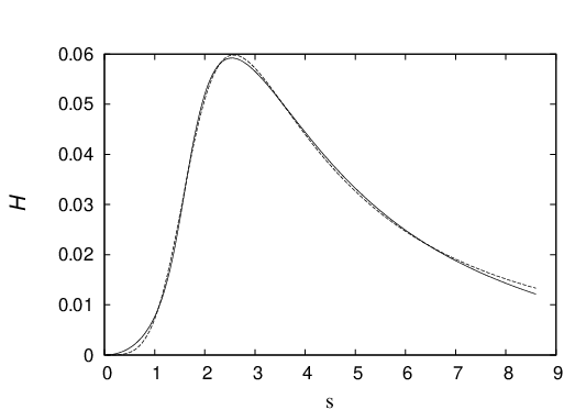
Here $F^{PBEsol}_{x}(s)$ is the PBEsol enhancement factor.[12] The integrals of Eqs. (11) and (12) can be solved analytically, [6] and Eqs. (11)-(13) reduce (by substitution) to an implicit equation for $\mathcal{H}$ [Eq. (A4) of Ref. 6]. We have solved this equation for PBEsol; the numerical solution that we have found for $\mathcal{H}(s)$ (see Fig. 2) can be fitted to the following analytic expression:

where $a_{1}=0.00018855$, $a_{2}=0.00741358$, $a_{3}=0.05687256$, and $a_{4}=0.00675093$. For $s>8.5$, as occurs in the tail of an atom or molecule where the electron density is negligible, the implicit equation for $\mathcal{H}(s)$ does not have a solution (as in the PBE case [6]) so we reset $s$ to $s=8.5$. Recently, Henderson et al. [21] constructed a GGA exchange hole that eliminates this unphysical large-$s$ behavior by using some ideas from the meta-GGA hole [7].

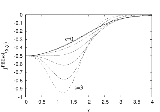
In Fig. 3, we plot the dimensionless exchange hole shape $J^{PBEsol}(s,y)$ [using the analytical fit of Eq. (14)] versus $y=k_{F}u$ for several values of the reduced gradient $s$. Our $J^{PBEsol}(s,y)$ looks similar to the $J^{PBE}(s,y)$ of Ref. 6, but $J^{PBE}(s,y)$ is deeper because $\mu^{PBE}_{x}=0.2195>\mu^{PBEsol}_{x}=0.1235$.

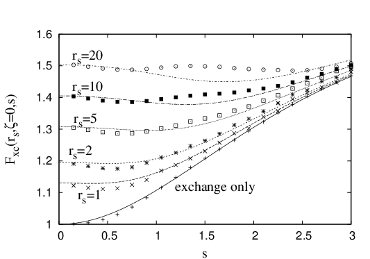
Finally, we look at the xc enhancement factor, which displays the nonlocality: [22]

$\epsilon_{x}^{unif}(n)$ being the exchange energy per particle of a spin-unpolarized uniform electron gas. For a spin-unpolarized system in the high-density limit ($r_{s}\rightarrow 0$) the exchange energy is dominant and Eq. (15) defines the exchange enhancement factor $F^{GGA}_{x}=\epsilon^{GGA}_{x}(n,\nabla n)/\epsilon^{unif}_{x}(n)$. In Figs. 4 and 5, we show the PBEsol enhancement factor for a spin-unpolarized system, $F^{PBEsol}_{xc}(r_{s},\zeta=0,s)$, and for a fully-spin-polarized system, $F^{PBEsol}_{xc}(r_{s},\zeta=1,s)$, versus $s$ for several values of $r_{s}$. $F^{PBEsol}_{xc}$ is calculated either (i) from the analytic expression of $\epsilon_{xc}^{PBEsol}$ reported in Ref. 12 or (ii) from our PBEsol angle-averaged xc hole density through Eq. (2). Overall, these calculations of $F^{PBEsol}_{xc}$ agree well with each other, confirming the assumption made at the beginning of this section; only for $r_{s}\geq 10$ (when the electron density is very small) and $s\approx 1.5$ is the error introduced by the second procedure significant [23]. The analytic fit for $\mathcal{H}(s)$ used to construct our PBEsol exchange hole does not exactly reproduce the PBEsol enhancement factor, but the difference is small as shown in Fig. 4. At this point, we also note that the parametrization[4, 12] of $H(r_{s},\zeta,t)$ entering the analytic expression of $\epsilon^{PBEsol}_{c}$ reported in Ref. 12 does not reproduce exactly the real-space cutoff results, as shown in Figs. 7 and 8 of Ref. 5.

The xc surface energy, $\sigma_{xc}$, can be defined as the xc energy cost per per unit area to create a planar surface by cutting the bulk. In a jellium model, in which the electron system is translationally invariant in the plane of the surface, and assuming the surface to be normal to the $z$-axis, the surface energy can be written as follows[3]

where[24]

is the wavevector-resolved xc surface energy, and

Equations (16)-(18) comprise an angle-averaged three-dimensional wavevector analysis of the surface xc energy into contributions from density fluctuations of various wavevectors $k$, following from the Fourier transform of the Coulomb interaction in Eq. (2). In these and subsequent equations, $k_{F}=(3\pi^{2}\bar{n})^{1/3}$ is the bulk (not the local) Fermi wavevector, and $r_{s}$ is the bulk (not the local) density parameter.

The exact low-wavevector limit of $\sigma_{xc}$ is known to be[2]

where $\omega_{p}=(4\pi\bar{n})^{1/2}$ and $\omega_{s}=\omega_{p}/\sqrt{2}$ are the bulk- and surface-plasmon energies, and $\bar{n}$ is the bulk density. Eq. (19) was used in the wavevector-interpolation approach reported in Refs. 2, 7, and 25, and it was naturally recovered by the RPA approach reported in Ref. 3.

Taking into account that $\bf{k}\equiv(\bf{k_{||}},\bf{k_{z}})$, $\bf{k_{||}}$ being a wavevector parallel to the surface, Eq. (18) can be expressed as follows[3]

In the case of RPA and TDDFT calculations, we use the fluctuation-dissipation theorem[26, 2, 27] to derive $n_{xc}(k_{\parallel};z,z^{\prime})$ and $\bar{n}_{xc}^{unif}(k)$ from the coupling-constant dependent density-response functions $\chi_{\lambda}^{unif}(k)$ and $\chi_{\lambda}(k_{\parallel};z,z^{\prime})$, as follows [3, 28]

and

$\chi_{\lambda}^{unif}(k,\omega)$ and $\chi_{\lambda}(z,z^{\prime};k_{\parallel},i\omega)$ being 3D and 2D Fourier transforms of the corresponding density-response function $\chi_{\lambda}({\bf r},{\bf r}^{\prime};\omega)$. In the framework of TDDFT (our benchmark for this work), the density-response function $\chi_{\lambda}({\bf r},{\bf r}^{\prime};\omega)$ satisfies a Dyson-like equation of the form[29]

where $\chi_{0}({\bf r},{\bf r}^{\prime};\omega)$ is the density-response function of non-interacting KS electrons (which is exactly expressible in terms of KS orbitals [30]) and $f_{xc,\lambda}[n]({\bf r},{\bf r}^{\prime};\omega)$ is the unknown $\lambda$-dependent dynamic xc kernel. When $f_{xc,\lambda}[n]({\bf r},{\bf r}^{\prime};\omega)$ is taken to be zero, Eq. (29) reduces to the RPA density-response function. If the interacting density response function $\chi_{\lambda}({\bf r},{\bf r}^{\prime};\omega)$ is replaced by the noninteracting KS density-response function $\chi_{0}({\bf r},{\bf r}^{\prime};\omega)$, then Eqs. (23) and (26) yield their exchange-only counterparts.

In the calculations presented below, we have considered, as in Ref. 3, a jellium slab of background thickness $a=2.23\lambda_{F}$ (where $\lambda_{F}=2\pi/k_{F}$) and bulk parameter $r_{s}=2.07$. This slab corresponds to about four atomic layers of Al(100).

For the GGA calculations of $\gamma_{xc}(k)$, the function $b_{xc}(k,z)$ entering Eq. (17) is taken from Eq. (18) with the xc-hole densities calculated as reported in (i) Ref. 20 for $\bar{n}_{xc}^{unif}(u)$, (ii) Refs. 5 and 6 for $\bar{n}_{xc}^{PBE}(z,u)$, and (iii) Section II above for $\bar{n}_{xc}^{PBEsol}(z,u)$.

For the exact-exchange, exact-RPA, and TDDFT calculations of $\gamma_{xc}(k)$, the function $b_{xc}(k,z)$ entering Eq. (17) is taken from Eq. (22) with the xc hole densities calculated from Eqs. (23) and (26). In the case of the TDDFT calculations, we use the accurate static xc kernel reported and used in Ref. 31. This kernel, which is based on a parametrization[32] of the diffusion Monte Carlo (DMC) calculations reported in Ref. 33 for the uniform electron gas, was constructed for jellium surfaces where neglect of the $\omega$-dependence does not introduce significant errors, and is expected to yield exact results in the limits of small and large wavevectors. Our numerical scheme was described in detail in Ref. 3, where only RPA calculations were reported.

The wavevector-resolved exact-exchange surface energy $\gamma_{x}(k)$ is shown in Fig. 6. Figures 7-8 and Fig. 9 show, respectively, the wavevector-resolved xc and correlation-only surface energies $\gamma_{xc}(k)$ and $\gamma_{c}(k)$. Figure 6 shows that $\gamma_{x}^{PBEsol}(k)$ improves over PBE, as expected, and is close to the exact $\gamma_{x}(k)$ for intermediate values of the wavevector. At large values of the wavevector, both PBE and PBEsol correctly recover the nonoscillatory LSDA (see Figs. 1 and 2 of Ref. 3); differences between this nonoscillatory PBEsol (and also LSDA and PBE) and the exact $\gamma_{x}(k)$ at these large values of $k$ are due to inaccuracy of the nonoscillatory model employed in Eq. (10) near $k=2k_{F}$.

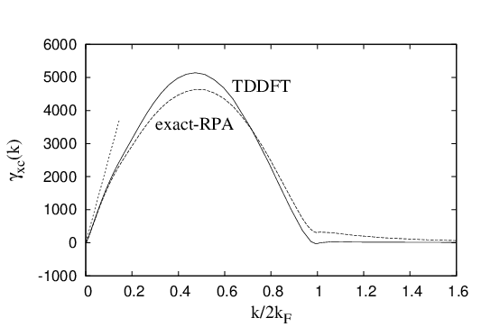
In Fig. 7, we compare the wavevector-resolved exact-RPA surface energy (as reported in Ref. 3) with its TDDFT counterpart (which we have not reported elsewhere, and which required three months of computation). In the long-wavelength limit ($k\to 0$), both RPA and TDDFT calculations approach the exact low-wavevector limit of Eq. (19). In the large-$k$ limit, where RPA is wrong, our TDDFT approach (which reproduces accurately the xc energy of the uniform electron gas) is expected to be accurate. Furthermore, the uniform-gas-based isotropic xc kernel that we use in our TDDFT calculation has been shown recently to yield essentially the same two-dimensional (2D) wavevector analysis as a more sophisticated high-level correlated approach (the inhomogeneous Singwi-Tosi-Land-Sjölander method) which does not use an isotropic kernel derived from the uniform gas.[34] Hence, we take the TDDFT wavevector-resolved surface energy represented in Fig. 7 by a solid line as the benchmark curve against which we compare various GGA’s.

Figure 8 shows our wavevector-resolved TDDFT surface energy together with its PBE and PBEsol counterparts. $\gamma_{xc}^{PBEsol}$ is nearly exact at small wavevectors, where it matches the exact initial slope of Eq. (19). At intermediate wavevectors, $\gamma_{xc}^{PBEsol}$ is very close to our benchmark TDDFT calculation. As in the case of wavevector-resolved exchange-only surface energies, PBE and PBEsol calculations correctly recover the nonoscillatory LSDA and differ from the more accurate TDDFT calculation due to the inaccuracy of the nonoscillatory model of the exchange-hole shape [see, e.g., Eq. (10)]. Figure 8 shows that $\gamma_{xc}^{PBEsol}$ nicely matches our benchmark TDDFT calculation at low and intermediate wavevectors, so we recommend using the model PBEsol xc hole, in all solid-state calculations where the hole is needed but full nonlocality is not important, instead of the more expensive TDDFT. We recall that the system-averaged hole, unlike the energy density, is uniquely defined, and is an observable at full coupling strength [5].

Figure 9 exhibits the wavevector-resolved correlation-only PBE, PBEsol, exact-RPA, and TDDFT surface energies. We observe that at long wavelengths ($k\to 0$), where the LSDA is known to fail badly, and at short wavelengths (large $k$), where RPA is wrong, the GGA’s under consideration are considerably close to our benchmark TDDFT calculations. At intermediate wavevectors, however, GGA’s cannot describe $\gamma_{c}$ accurately, although PBEsol has been shown in Fig. 8 to give a very good description of $\gamma_{xc}$. This is due to a cancellation of the errors introduced at these wavevectors within the exchange and correlation contributions to $\gamma_{xc}$, which almost cancel each other [35].

We have constructed a PBEsol angle-averaged xc hole $\bar{n}_{xc}(\mathbf{r},u)$ that satisfies known exact constraints and recovers the recently reported PBEsol xc energy functional. Our construction of the PBEsol xc hole begins from and appropriately modifies the sharp cutoff correlation hole of Ref. 5 and the smooth exchange hole of Ref. 6. We also generalize [see Eq. (7)] the sharp cutoff procedure for the correlation hole to any GGA which has a positive gradient expansion coefficient.

We have found that our PBEsol xc hole describes accurately the wavevector-resolved xc jellium surface energy for all values of the wavevector, thus providing support for the PBEsol GGA for solids and surfaces.