[current]last ection]chapter .4pt[]
![[Uncaptioned image]](0901.3617v1/logo.png)
A parton recombination approach to heavy ion collisions at RHIC and LHC
Diploma thesis
by Daniel Krieg
December 2008
Für Daniela
Contents
List of Figures
List of Tables
Chapter Introduction
. 1 Curiosity and doubt
The knowledge of mankind has grown rapidly in the last century. Especially through the fundamental research in physics. It was and is driven by human curiosity, since typically the fundamental research has no direct application in everyday or technical life. Nevertheless, over the time these insights into natural laws have shown their profitableness in the technical revolutions.
So on the one hand, the growth of the knowledge of mankind has always been driven by curiosity, since ‘‘curiosity is always the starting point for solutions to a problem’’11 1 Galileo Galilei. On the other hand, physical models and theories can never be right or true in a rigourous sense, but only falsified. So beside our success in describing nature, ‘‘we absolutely must leave room for doubt or there is no progress and no learning. There is no learning without having to pose a question. And a question requires doubt’’22 2 Richard P. Feynman, Galileo Symposium in Italy, 1964. In order to learn about nature, we have to be curious and ask new question, but we also must have the courage to doubt our new found answers.
But curiosity is not a feature of science itself, it is an innateness of mankind. Most of the questions asked by physicists may seem academic and irrelevant to the scientific layman. Maybe still complicated, the questions that are tried to be answered by nuclear phyicist, by colliding atomic particles at the speed of light, are those questions every human reflects: Where are we from and why are we here?
Where we are from is widely believed to be the so called big bang, during which time, space, matter and energy turned into existence. Why or what exactly happend at time zero no one can tell because at this singluarity in spacetime the law of physics broke down. Asking about before also makes no sense, because without time there is no before.
Why we are here is a more philosophical question which can be understood in many different ways. While the physicist wonders about the asymmetry between matter and antimatter, which is an essential fact for our existence, others would ask this question more spirtiually. But the creation of the universe via a big bang would not contradict the existence of an omnipotent power that is responsible for ‘‘life, the universe and everything’’33 3 Douglas Adams, The Hitchhiker’s Guide to the Galaxy…
. 2 The fundamental building blocks
But let us go back to a question we believe to have answered to a wide degree: What are we made of? This question has a long history and mankind has had great success in finding the fundamental building blocks that make up the matter around us. Most all of these findings where mainly made in the last century.
The theory of the greek classical “elements” earth, water, air and fire, that go back to the philosopher Empedokles, persisted to the sevententh century until the new definition for an element by the chemicist Robert Boyle marked the beginning of the modern chemistry.
The chemicists classified many new elements, which soon required a new ordering schema. The periodic system of the elements was introduced which sorts the elements by their mass and attributes to groups of eight. The electron, the first subatomic particle, was discovered in 1897 by Joseph John Thomson while its existence was predicted by George Johnstone Stoney 23 years before. Thomsons so-called “plumpudding”-model of the atom was replaced in 1911 by Ernest Rutherford after his famous scattering experiment. With Rutherfords interpretation, where a positively charged core is surrounded by a cloud of electrons, it was then possible to explain the chemical properties in the periodic system by the atomic electron shells. In 1919 Rutherford discovered the proton, and with the discovery of the neutron in 1932 by his student James Chadwick the description of the atomic nuclei was complete. On the one side, the atomic physics focused on the electron shells, Max Born postulated discrete orbits for the electrons and with the advent of quantum mechanics physicists were able to explain the atomic spectra.
On the other side the nuclear physicists were studying the structure of the atomic core. Around the 50’s more and more new particles like the proton and neutron, called hadrons, were found. Soon there was such an overwhelming richness, that now the nuclear physicists needed a new ordering schema. Murray Gell-Mann proposed his “eightfold-way”, where the hadrons could be grouped to octets of similiar mass. This was the predecessor of the quark model in which the protrons, neutrons and all other hadrons are no elementary particles, but made up of quarks, where the mesons are quark-antiquark combinations and the baryons consist of three quarks.
Today the standard model of particle physics classifies the fundamental particles into fermions as the particles of matter and the bosons as the particles mediating the interactions. The standard model (SM) has been very successful and marks a milestone in our understanding of the elementary particles and their interaction. But it falls short of being a complete theory since it lacks the description of gravity. Also the many free parameters that have to be determined by experiment are a big shortcoming of the model.
So there are many attempts to extend the SM (e.g. supersymmetry) or to discard it in favor of a new theory (e.g. stringtheory). But up to now it is the best answer to the question “What we are made of”.
. 3 Back to the Big Bang
When we go back in time, we can see different forces responsible for the evolution. At the beginning the universe was extremly hot and dense and all fundamental particles were unbound and free like in plasma. Due to the expansion the temperature was going down and the quarks were pulled together by the strong force and formed hadrons; this is called hadronization. Most of them are unstable, but protons and neutrons assembled to stable clusters. During the ongoing cooling the electrons were bound to these clusters by the electromagnetic force. The atomic elements and molecules began to develop. Finally, the gravity pulled the neutral atoms together and so larger clusters of matter started to grow forming the stars and planets making up our known universe.
The gravity and the electromagnetic force are quite good understood, so one main topic of current research is the study of early universe, the regime of the strong force. In fact, this force is so strong that it is not possible to separate two quarks. Therefore, no one has ever seen (or measured) a quark. The hope is that if we could heat up the hadrons to the temperatures directly after the big bang, we could create this plasma state of the quarks where they are free. With the largest machines in the world, physicists collide nuclei at the speed of light to create such a hot and dense system resembling the universe a few nanoseconds after the big bang to study the phase transition of the strongly interacting matter. The theoretical description of these collisions are very involved and due to the complex dynamics of the fundamental degrees of freedom, this is not yet understood from first principles.
In this thesis, I will analyze a phenomenologial model called recombination or coalescence which is a relevant mechanism for hadronization in heavy ion collisions (HIC) at the highest energies that are available today. It is structured as follows:
- •
In the next chapter I give a short introduction into the phenomenology HIC, explain different models to describe the collisions and discuss how to probe the QGP.
- •
The third chapter adresses the hadronization from a QGP, focusing on the recombination approach and its ingredients.
- •
The results are presented in chapter four where I first give an overview of the parameters and parameterizations, followed by a detailed discussion on the different results and predictions of recombination.
- •
The last chapter contains final remarks and conclusions.
Chapter Heavy Ion Collisions
. 4 Phase diagram of the strong force
The main goal of the current and past heavy ion programs is the search for a new state of matter called the Quark-Gluon-Plasma (QGP) Bas [99]. The quarks are the constituents of hadrons. They interact via their color charge by the strong force meditated by the gluons. Due to the strong coupling quarks can not be observed as single particles, only as clusters, where the color of all quarks add up to “white”. This so called confinement is expected to break at sufficiently high temperatures and/or densities. The quarks and gluons are then free unbound particles like the electrons and protons in a plasma. That is why this state of matter is referred to as QGP and describes a new phase different to the normal ground state.

The nuclear matter in the accelerators is highly compressed and heated up during the collision. At suffienctly high beam energies, we expect the system to go through a phase transition from the hadronic phase to the QGP. Due to the large pressure, the systems expands rapdily, cools down and crosses the phase boundary again. The quarks hadronize and form new hadrons. In this still very dense system, the hadrons scatter mostly inelastic and create exited hadronic states until the system is too dilute. At this so called chemical freeze-out, the inelastic cross sections are neglectable. After the kinetic freeze-out, there are also no more elastic interactions between the hadrons.
The livetime of the QGP is very short and only the hadrons coming from the kinetic freeze-out can be measured in the detectors. So there is no way to see if we have created a QGP or not. There are two different ways to examine the early phase of the collision:
- •
We can study different probes that can escape the early system mostly undisturbed and try to extract information from these measures. That would be particles with a low cross-section in the medium like photons, pair-created leptons (dileptons) and heavy-quark mesons ().
- •
The other possibility is to look for characterisitic properties of the hadrons from freeze-out, which can be associated with a QGP formation, e.g. collective flow phenomena like the elliptic flow.
. 5 Theoretical descriptions of heavy ion collision
. 5.1 Statistical thermal model
The thermal model is a statistical approach to particle multiplicity in heavy ion collisions. One assumes a globally equilibriated thermal source described by temperature and chemical potentials for the charges . The thermodynamical observables are then evaluated as an average over the statistical ensembles BM [03]. Therefore, one has to calculate the grand canonical partition function
| (1) |
where the Hamiltonian depends on the equation of state (EoS), which connects the energy density with the pressure. The EoS depends on the degrees of freedom and so changes throughout the evolution of the system. The EoS of the QGP is subject to current research and can only be determined within QCD. Below the phase boundary the system can be described by a hadron resonance gas with a known EoS.
The applicability of the thermal model is very limited. The assumptions of global equilibrium and a static source are at best questionable. The predicted particle multiplicity, when using the EoS of the hadron gas, are in good agreement, but since this does not require the formation of a QGP, the predicitve powers are very limited.
. 5.2 Quantumchromodynamics (QCD)
The only possibility to really calculate the shape and order of the phase transition would be to solve the equations of motion for QCD, the gauge theory for the strongly interacting colored particles. The approach from Quantumelectrodynamics (QED), where pertubation theory is very successful because of the small coupling constant , is barely applicable in QCD due to the large coupling of the strong force and the non-abelian nature of the corresponding symmetry group . The pertubative QCD (pQCD) works only at large momentum transfers, where the running coupling constant becomes small.
The other way is to discretize the langrangian and solve it numerically on a lattice (LQCD). Since this requires vast computational powers, there is no chance of a dynamical description from LQCD. But it can give insights into the order of the phase transition, the critical energy density and the equation of state Fod [02], dF [06], Ste [06]. These are needed as input to hydro- and thermodynamical models.
Due to the lack of lattice data at high baryo-chemical potentials, I will later use the simple phenomenological MIT bag model to describe the confinement and the phase transition.
. 5.2.1 Fragmentation (pQCD)
The hadron production at sufficiently large momentum transfer can be described by pQCD. The quark-antiquark pairs created in hard scatterings are connected by a color string and as they depart from each other back to back, the potential energy between them rises until the string breaks and creates a new quark-antiquark pair. This process continues until most of the kinetic energy of the original parton is converted. The hadrons, formed from the created quarks, carry a momentum fraction of and are all emitted in the direction of the original parton. This is called a jet.
The probability that the jet of parton emits a hadron with a momentum fraction is called fragmentation function and can be measured in annihilations. The invariant cross section for a hadron with momentum can then calculated with
| (2) |
For proton-proton collisions the situation is comparable to the annihilations, but in heavy ion collisions (A-A collision) with a large fireball volume, the jets lose energy as they travel through the medium and will be modified. This modification is prominently observed in the so-called away-side jet supression: When two partons are created near the edge of the fireball, one jet can be emitted directly into vacuum while the other one has to travel through the whole dense medium and will therefore be suppressed.
But for a dense medium, the description in terms of a jet from a single quark is questionable and one has to account for multiple parton fragmentation (higher twist). In the extreme case of a very dense phase space with abundant quarks, they might simply recombine. That means e.g. if a and quark are near in phase space, they are confined to form a . This recombination mechanism plays an important role in the mid- range while it is dominated by fragmentation at high-. I will dicuss the recombination (also called coalescence) approach in the next chapter.
. 5.2.2 MIT bag model
In the MIT bag model Cho [74], Cho [75], Myh [84], The [80] the quarks and gluons are confined in volume with radius equal to the radius of a nuclei. Outside of this volume, the virtuell quark-antiquark-pairs excert a pressure on this bag, which prevents the partons inside to escape. They can be described by thermodynamics as ideal gas.
The pressure of this gas depends on the temperature and the density which is expressed by the chemical potential . If this pressure becomes greater than the bag pressure, the partons inside can escape their confinement.
So the phase boundary 44 4 The derivations of this formula can be found in the appendix A. within the bag model is at
| (3) |
with and the critical temperature at zero chemical potential.
. 5.3 Transport theory
The transport model Bas [98], Ble [99] is a microscopic approach which models the trajectory of every single particle. The evolution of the system is calulated with the Boltzmann equation
| (4) |
where the collision term depends on the cross-sections and determines the time-dependence of the distribution function. Since only two-body collisions are considered in the gain and loss terms, one has to assume a dilute gas of particle with large mean free path so that three- or more-body collisions are neglectable. But the advantage is that since it is a microscopic theory, it can describe non-equilibrium systems.
. 5.4 Hydrodynamics
The complement to transport theory is hydrodynamics, where one assumes a local equilibrium within a dense system, e.g. a very small mean free path of the particles like in a fluid. It is a very common model in HIC Kol [03], Kol [00], especially, since the matter created at the Relativistic Heavy Ion Collider (RHIC) seems to behave like a perfect fluid (minimal viscosity) Rom [07], Tan [06].
With the equilibrium assumption, we can set the collision term in eq. (4) to zero, and with the baryon number current and the energy-momentum tensor , the basic formulas read
| (5) | ||||
| (6) |
State-of-the-art calculations are 3-dimensional with three distinct fluid, e.g. two for the colliding nuclei and a third for the evolving collision zone. For simpler systems the equations can be solved analytically which has been done by Bjorken Bjo [83] and Landau Lan [53].
The hydro results depend on the needed input, namely the initial conditions (Glauber model or CGC), the equation of state (LQCD) and the freeze-out prescription.
. 5.4.1 Collision geometry
The interpretation of the time evolution of the system in the transverse plane is motivated by hydrodynamical ideas. The high compression of the nuclear matter generates a high pressure in the fireball. The difference of the inner medium and the surrounding vaccum results in a pressure gradient. This leads to an expansion in the transverse direction. The initial transverse area, determined by the overlap zone of the nuclei, increases rapidly until the freeze-out. So the spectrum of the particles can be described by the emission from a boosted thermal source, where the transverse velocity of the particles comes from the thermal motion with a superimposed transverse boost.
Based on these ideas, the particle spectra are fitted by the so-called blast-wave model that describes a thermal source with a transverse and a longitudinal boost. Because the longitudinal rapidity is generally taken to be equal to the space-time rapidity by invoking Bjorkens longitudinal boost invariance, the model is characterized by three parameters namely temperature , baryo-chemical potential and transverse expansion rapidity .
For collisions with non-zero impact parameter the radial size and therefore the pressure gradient varies with the azimuthal angle . It is defined with respect to the plane in which the nuclei collide. The direction with or is called “in-plane” and perpendicular to that “out-of-plane” (Fig. 2(a)). The protons and neutrons in the collision area that will take part in the scattering are called “participants”, while the other nucleons, which just pass by, are called “spectators”.
The radial size in-plane is smaller than out-of-plane which leads to a larger in-plane pressure gradient. The spatial azimuthal asymmetry therefore generates a momentum asymmetry that is perpendicular to the spatial one (Fig. 2(b)).
During the expansion, the increasing momentum asymmetry weakens the spatial asymmetry and so destroys its own origin; it is self-quenching. So the spatial eccentricity at freeze-out will differ from the initial one (Fig. 2(c)). Depending on the hydrodynamical evolution and the freeze-out time it can be smaller, zero or even negative. A negative freeze-out eccentricity would mean a change of direction from an elongation out-of-plane to in-plane.


Chapter Hadronization from a QGP
In the previous chapter, I shortly discussed different theories for the description of heavy ion collisions and the phase diagram of the strong force. Currently, the collision dynamics are studied extensively within microscopical transport theory and hydrodynamics while the location and nature of the phase transition is subject to research in lattice QCD.
The main question of my thesis is, assuming we have crossed the phase border in a HIC and created a QGP, how do the quarks form hadrons again when the plasma cools down. Therefore I will analyze an analytic model for the colinear recombination approach Fri [03]. Beside studying probes from the early phase of the collision, this offers the possibility to study the influence of a QGP creation on different observables at the freeze-out.
This chapter has the following structure:
- •
The first section contains the recombination formalism,
- •
the second one addresses the form of the hypersurface where the phase transition and freeze-out take place,
- •
the third one introduces the blast-wave model which models the quark densities depending on the collision geometry and
- •
the fourth section will contain the formulas for the observables from the recombination approach with the quark density and freeze-out hypersurface as dicussed.
. 6 Colinear recombination of quarks
. 6.1 Introduction
The results from the Relativisitic Heavy Ion Collider (RHIC) are a confirmative sign for a very dense phase space so that recombination seems to play a major role in the hadronization process. While the strong nuclear suppression (ratio of A-A to p-p collisions) of pions is widely seen as the experimental confirmation of jet quenching predicted by pQCD, there are several key observations that cannot be explained by fragmentation. These are the very different results for mesons and baryons namely
- •
the nuclear suppression factor,
- •
the elliptic flow and
- •
the large baryon / meson ratios.
For collisions with a higher center-of-mass energy, the influence of recombination can be expected to be even higher. The predictions for the Large Hadron Collider (LHC) are therefore of great relevance.
I will now discuss the implications of an analytical coalescence formalism that constrains the recombining quarks to have colinear momenta. For a detailed discussions of the derivations I refer to Fri [03]. While the onset of fragmentation sets the upper bound of applicability, the colinearity constraint leads to an energy violation at low . Therefore, the results for the transverse momentum spectra of this recombination model will be valid only for . But the most prominent and promising observable of recombination, namely the elliptic flow , can be expected to give valid results down to several hundred MeV Fri [03], since the azimuthal angle dependence in these flow coefficients is only expressed relatively to the absolute yield. And also the very good description of the data (see sec. . 13.4) justifies the use down to low . So such an analytical model can still serve as a good guidance in studying the general features and point the way for dynamical studies.
. 6.2 Non-relativistic model
Let us start with a volume V with a homogen distribution of various quarks which will therefore only depend on the momentum. We assume that only constituent quarks with colinear momentum will recombine to form a hadron with momentum . This simple picture then leads us to a first non-relativistic equation for the hadron multiplicity which is the momentum integral over the product of the quark densities times the probability for these quarks to form a hadron (namely the wavefunctions overlap squared). For simplicity, I will stick to mesons (quark-antiquark pairs) and will give the generalization to baryons later. The spatial wavefunctions for the quarks and the meson are:
| (7) |
| (8) |
Defining the center of mass and relative coordinates resp. momentum as and resp. and , the overlap is
| (9) |
is then the fourier transform in the relative momentum. Due to the absolute value squared, the deltafunction has to be rewritten as
| (10) |
Using this in the proposed formula for the hadron multiplicity
| (11) |
with a spin degeneracy factor (mesons) or (baryons) respectively, one finds the momentum distribution
| (12) |
Assuming an exponential parton distribution , the -dependence will drop from the density product. Due to the normalization of the wavefunction, the integral vanishes and one is left with
| (13) |
The spectrum does not depend on the form of the wavefunction, it is just exponential. The only dependence on the specific hadron is in the degeneracy factor and the quark fugacities .
Even in this simple approach one can explain the large baryon/meson ratio at RHIC, which pQCD fails to predict. It simple comes down to the degeneracies
| (14) |
which then results a proton-to-pion ratio of about 2, in contrast to about 0.2 from pQCD fragmentation.
. 6.3 Relativistic
To make the approach more general and consistent, one starts from a density matrix for the quarks and . The number of mesons is then given by
| (15) |
Inserting complete sets of coordinates
| (16) |
and using the definition of the wigner function
| (17) |
With the center of mass (c.m.) coordinate and the relative coordinate of the correlation coordinates, one can define the relevant quantities for the hadron. By assuming small spatial variations in the wigner function, after some steps one arrives at
| (18) |
with the relative momentum between the quarks, the spatially integrated wigner function of the meson and the future orientated unit vector on the freeze-out hypersurface . When going to local light cone (LLC) coordinates, one can restrict the quark momentum to colinearity by writing it as a fraction of the hadron momentum. By introducing the ansatz for the light cone wavefunction
| (19) |
the formula for the invariant yield becomes
| (20) |
with , the number of constituent quarks and
| (21) |
In the case of quarks this is simplified to
| (22) |
As already shown in the previous section, the recombination formalism alone is capable of explaining the large baryon/meson ratio, but the results will generally depend strongly on the parameterizations of freeze-out hypersurface and the used quark density .
. 7 Freeze-out
Now I will model the freeze-out hypersurface. The spatial four-vector
| (23) |
will be translated into the new coordinates
| (24) |
with the transverse radial variable , its angle , the time and the space-time rapidity
| (25) |
For the study of collisions with a nonzero impact parameter, I will directly generalize to an ellipsoidal cylinder. The elliptic transverse freeze-out area
| (26) |
has the numerical eccentricity
| (27) |
if . To avoid ambiguities with other eccentricity definitions, the numerical eccentricity of an ellipse with the above definition will be called while the denotes the freeze-out value.
So the surface radius depends on the angle , which is measured with respect to the x-axis:
| (28) | ||||
| (29) | ||||
| (30) | ||||
| (31) |
The radial coordinate is constant for a given ellipsoid surface. The length of the short axis (in-plane) and respectively the long axis (out-of-plane) are
| (32) | |||
| (33) |
The constant is chosen such that the transverse area is independent of the eccentricity and only depends on the parameter . From
| (34) |
if follows
| (35) | ||||
| (36) |
Looking at eq. (29), one directly sees that the axes are changed under the transformation and the ellipsoid is flipped by . This will be used in the next paragraph.
. 7.1 Integration measure
To obtain a 3-dimensional freeze-out hypersurface, one needs to apply a constraint to the four-vector or respectively . This is done by constraining the freeze-out time to be a function of the other three variables, so generally .
The simplest choice would be to use a constant freeze-out time with , but to be a bit more general and to connect the transverse with the longitudinal dynamics, I will perfom the derivations with an explicit dependence only.
According to the Cooper-Frye prescription Coo [74] the integration measure is given by
| (37) |
where is the normalvector on the hypersurface in the new coordinates which is calculated by a generalized cross-product of the tangent vectors. Therefore, I will calculate the Jacobian
| (38) |
With the dependencies
| (39a) | ||||
| (39b) | ||||
| (39c) | ||||
| (39d) | ||||
the tangent vectors read
| (40a) | ||||
| (40b) | ||||
| (40c) | ||||
where
| (41) |
With the fully anti-symmetric rank-4 tensor , the infinitesimal normalvector on the hypersurface is calculated as
| (42) |
Similiar to eq. (39), the particle momentum is parameterized as
| (43) |
which then leads to the integration measure
| (44) |
If I had assumed a constant independent of , the second term would vanish and the integration measure would simplify to
| (45) |
By additionally setting , one recovers the measure for a cylindrical freeze-out, since
| (46) |
. 7.2 Surface flow
For an ellipsoid the radial direction is generally not perpendicular to the surface. It is related to the orthogonal direction by
| (47) |
So for an elliptical freeze-out area I consider the two extreme cases:
- •
Model 1: the system expands perpendicular to the surface
- •
Model 2: the system expands radially outwards independent of the surface orientation

Fig. 3 depicts the possibilities. When I drop the dependence of (eq. (45)) both models can be related via the integration measure Tom [05] as can be shown by rewritting the and coordinate in eq. (39) using the angle :
| (48) |
and similar
| (49) |
The integration measure becomes
| (50) |
which is similiar to the one from eq. (45). When renaming , the only difference is the transformed . As already explained above, this transformation is a rotation of the ellipse by . So the integration over an ellipse elongated out-of-plane with the system expanding perpendicular to the surface is equal to the integration of an in-plane ellipse with a radial expansion. But this exact correspondence is only true if . The consequences of this relation are discussed in section . 11.3.1.
. 8 Blast Wave Model
For the parameterisation of the partonic density I take inspiration by hydrodynamical ideas Sch [93], Flo [04] and therefore assume a locally thermalised fireball. With the four-momentum of the quark and the flow four-velocity of the system , the thermal density for fermions with the degeneracy factor reads
| (51) |
To simplify the derivations, I only use the lowest-order term which is just Maxwell-Boltzmann statistic. This is sufficient, since the higher order terms are neglectable as I have verified.
. 8.1 Azimuthal momentum asymmetry
In hydrodynamics the transverse flow is generated by a pressure gradient
| (52) |
which will depend on the angle for non-central collisions. The spatial asymmetry (fig. 2(b)) has the initial numerical eccentricity
| (53) | |||
| (54) | |||
| (55) |
of an ellipse with the long axis (y-direction) and the short axis (x-direction) which describes the collision in the transvese plane and only depends on the impact parameter . So in the x-direction there is a stronger pressure gradient as in the y-direction. This yields a larger expansion velocity of the system and this momentum asymmetry will be perpendicular to the spatial asymmetry. This expansion leads to a decrease in the spatial asymmetry and therefore a decelerated growth of the momentum asymmetry which is called a "self-quenched" behaviour, since the momentum asymmetry destroys its own origin.
The size of the initial transverse area is determined by the impact parameter:
| (56) |
It is not a piori clear how the spatial eccentricity will evolve until the freeze-out, but it generally depends on the initial spatial eccentricity, so . Depending on the dynamics, the system could
- •
freeze-out early and leave a remaining spatial freeze-out eccentricity , where it is still elongated out-of-plane,
- •
freeze-out so that the initial spatial eccentricity has been compensated by the expansion and it is now circular with
- •
or freeze-out late so that the initial spatial eccentricity is overcompensated and reversed so it is elongated in-plane.
The second point is just a special case of first one. So one has to distinguish between the elongation of the spatial area at freeze-out. In section . 11.3.3 I will give evidence for the first option and also relate to to study the effects of a non-circular freeze-out area.
. 8.2 Comparing asymmetry parameters

I would like to state again that the used eccentricity is the numerical eccentricity of an ellipse while the eccentricity definition generally used in the heavy-ion community is Jac [00]
| (57) |
where the average is over the transverse plane weigthed by the nucleon density. For a simple constant density this is simplified to
| (58) |
The definition of this (lets call it "geometric") eccentricity differs from the definition of the numerical eccentricity . To compare one with the other, the above equation is written in terms of the numerical eccentricity.
| (59) |
Realistic calculations of the eccentricity are the ones from the glauber model Gla [70] which differs from the simple approximation , because it accounts for the thickness of the nuclei. Especially for very peripheral collisions, where only the sparsely populated parts of the nuclei collide, the glauber eccentricity is much smaller. Figure 4 shows a comparison for different conditions Hir [06], including the Color Glas Condensate (CGC) results. The value of is generally to large but is in good agreement with the glauber model. Therefore, I define the eccentricity by the relation
| (60) | ||||
| (61) |
The relevance of this redefined eccentricity becomes visible in the following paragraph.
. 8.2.1 Expansion velocity
Since the transverse flow is generated by a pressure gradient and I will not model the pressure profile, I take the ansatz from eq. (52) and assume with the mean transverse flow rapidity as a free parameter. To have a much more handy expression, I rewrite the denominator and expand it to fourth order in :
| (62) |
So the elliptic asymmetry scales mainly linear with the defined eccentricity
| (63) |
which is comparable to the glauber eccentricity from central to mid-central collisions as can be seen in Figure 4. This leads to a direct linear relation between the elliptic flow and the eccentricity which is also expect from hydrodynamics (see section . 13.2) and therefore justifies the choice in eq. 60.
Together with a radial profil in , the expression reads
| (64) |
The normalization is chosen to be so that
| (65) |
Now the four velocity of the expanding fireball is created with a longitudinal boost and a transversal boost . Taking Bjorkens boost-invariance argument, I set the longitudinal rapidity equal to the space-time rapidity, i.e. :
| (66) |
The angle depends on the model chosen for the surface expansion from section . 7.2 with for model 1 (perpendicular expansion) and for model 2 (radial expansion).
. 9 Observables from recombination
. 9.1 Invariant yield
Now I combine the recombination formalism with the discussed freeze-out hypersurface (sec. . 7) and the quark density from the blast-wave model (sec. . 8). With eq. (22) the invariant yield for the quarks read
| (67) |
where the exponent expands to
| (68) |
To study the dependence on the particles momentum angle , one uses the fourier expansion
| (69) |
with
| (70) | ||||
| (71) |
The -integrated yield describes the overall transverse momentum dependence, while the other fourier coefficients and encode the deviations from an azimuthal symmetric yield. To have a better comparison, the normalized fourier coefficients and , also called flow coefficients, are introduced:
| (72) | ||||
| (73) |
The full expression reads 55 5 How to solve the integrals can be found in the appendix B.
| (74) |
For the coefficients , one has to replace the cosine terms with sinus. From that the -integrated yield follows as
| (75) |
The arguments for the modified bessel functions and are
| (76a) | ||||
| (76b) | ||||
Due to the symmetry of the system, most coefficients vanish. The only dependence is in the function which only contains terms proportional to , as can be seen in eq. (62). Therefore, the expectation values and vanish:
| (77) | |||
| (78) |
This results in the symmetries
| (79) | ||||
| (80) |
For the hadrons the integration over the product of the quark densities involves an additional integral over the momentum fractions times the wavefunction (eq. (20)):
| (81) |
Due to the product , the arguments of the besselfunctions are now -weigthed sum of the above arguments (eq. (76)) for the quarks:
| (82a) | ||||
| (82b) | ||||
where is the number of valence quarks.
The degeneracy factor are not a priori clear from QCD. In principle every quark has 3 color and 2 spin degrees of freedom. But since there are no dynamical gluons in this model it would be consistent to require that the quarks have the right quantumnumbers. Therefore, the degeneracy is only determined by the degrees of freedom of the hadron, e.g. and . I will not take into account feeddown from resonance decay, except for the , where the is too close in mass to be suppressed. Hence I take Fri [03].
. 9.1.1 Central collisions
For collisions with zero impact parameter, the initial as well as the freeze-out eccentricity will be zero. Then and is independent of and so one arrives at
| (83) |
. 9.1.2 Peripheral collisions
The parameter measures the size of the transverse freeze-out area (see eq. (34)).
The total multiplicity depends on the initially created quark density, which I assume to scale linear with the size of the initial transverse area (eq. (56)), which only depends on the impact parameter . In order to have only one parameter for all centralities, I let scale like
| (84) |
and will fix for central collisions.
. 9.2 Flow components
. 9.2.1 Elliptic flow
The first non-vanishing fourier coefficient in the expansion is the so called elliptic flow which will therefore dominate the expansion. It measures the momentum asymmetry between the particles emitted in-plane (-direction) and out-of-plane (-direction):
| (85) |
For , it can be calculated by
| (86) |
The importance of this observable comes from the fact that it is generated by the self-quenching momentum asymmetry (see sec. . 8.1) and is therefore mostly sensitive to the initial (partonic) stage of the collision.
. 9.2.2 Hexadecupole flow
To study additional effects, I also take a look at the next order . By considering the ratio of the different coefficients, one can disentangle the different contribution to the flow. Since the coefficients scale like and , one expects the ratio of the flow coefficients to be independent of the initial eccentricity. In the section . 9.3.2, I will give a more detailed description of this ratio.
. 9.2.3 High- flow
The flow components calculated with recombination are monotonically rising with . Since I will not consider contributions from fragmentation which dominates over recombination at high , the experimental observed drop at a finite has to be modeled by a phenomenological factor Fri [03]
| (87) |
with the additional parameter . It enters the transverse flow rapdity (eq. (64)) and makes sure that faster partons do not feel the expansion asymmetry that much:
| (88) |
. 9.3 Constituent quark number scaling
. 9.3.1 Elliptic flow scaling
One major success of recombination is a predicted simple connection between the quark elliptic flow and the hadron elliptic flow which gives strong evidence for a QGP phase in the collision. This connection is called “constituent quark number scaling” (CQNS), because the hadron elliptic flow scales with the number of constituent quarks.
To study the connection of the elliptic flow between quarks and hadrons, let us fourier expand the quark density similar to eq. (69) as
| (89) |
by defining and .
To simplify the derivation, I take which is only a minor simplification compared to the following ones. Because of the orthogonality of the cosine, only the coefficient enters the elliptic flow for quarks:
| (90) |
To compare it to the hadron elliptic flow, I simplify the hadron wavefunction. Since it is the product of the momentum fractions , it is already maximal for quarks with equal momentum. Therefore, I use the delta-function approximation
| (91) |
Then the -integration will brake down and all quarks have the equal momentum fraction . For a meson one now has a product of two fourier series which can be expanded to
| (92) |
As I will show in section . 9.4, the higher terms can not be neglected, so analytically there is no simple and exact relation between the quark and the hadron .
Those who want to derive an analytical expression for the scaling, must use a strong simplification and drop the spatial correlations between the angle and flow velocity from the quark density. In this case, one assumes just a constant asymmetry in the flow profile which is equal at every point in the fireball, and rewrite the density with the help of the quark elliptic flow as Fri [03]
| (93) |
The azimuthal asymmetry is only contained in the term which depends only on the hadron emission angle . The previous dependence of on the spatial angle is now gone. When assuming a circular freeze-out area (), the -dependence can be integrated out completely which leads to a much simpler equation for the hadron elliptic flow. One finds for mesons
| (94) |
and for baryons
| (95) |
where is to be evaluated at for mesons and at for baryons. With the additional simplifications of a constant transverse flow rapidity independent of the radius, one arrives at
| (96) |
and
| (97) |
respectively. For hadrons with similiar quark content all coefficients are equal and by further neglecting quadratic and cubic terms, one obtains the much celebrated constituent quark number scaling Fri [03]
| (98) |
Beside all the simplifications, this scaling law is confirmed with great success by the experimental data. A common way to show the good agreement is to scale the data of hadrons by and plot it as vs. . According to the scaling law, all curves for mesons and baryons will lie on one universal curve which would be the quark elliptic flow.
. 9.3.2 Hexadecupole flow scaling
With the above simplifications, one can also derive a scaling law for the hadron . Again neglecting higher powers and assuming equal and for all quarks, one finds
| (99) |
and
| (100) |
Combining the both scaling laws, ratio between and can be expected to be approximately
| (101) |
and
| (102) |
. 9.4 The breaking of the CQNS
Although the CQNS is experimentally well observed, the scaling is broken by the masses of the hadrons and the simplified equations from the upper section ca not account for that. Therefore, I want to emphasize that the scaling laws will only serve as a rough guide and all calculations will be done with the full spatial correlations of the quark density, if not specified otherwise.
Let us shortly discuss the scale breaking terms: Taking the quark-antiquark density from eq. (92) the meson elliptic flow can be calculated via
| (103) |
and are the contributing terms from the infinite sum. Because of the orthogonality of the cosine, all terms not containing the integral weightings (i.e. for the denominator and for the numerator) have vanished after the -integration. With the trigonometric product
| (104) |
an infinite sum of coefficient products that fulfill or , contributes to
| (105) |
This leads to
| (106) |
and
| (107) |
In fig. 5 you see the comparison of the full calculation to zeroth order. In zeroth order, the terms contain only the contributions:
| (108) |
This would correspond to the CQNS. Obviously, the simple approximation of zeroth order is not sufficient when calculating with the full momentum space correlations. Therefore, the higher terms can not be discarded and a simple, analytical form for quark number scaling does not exist in this framework.

Additionally to the contribution from the higher order flow components, the bessel functions give further deviations from the scaling law: In the high region the additional powers of give an enhancement for the elliptic flow, so it will be higher than . The higher the higher the enhancement will be. On the other hand, in the low region where is approximately one, the scaling will be broken by . The argument is the sum over the transverse masses of the quarks at . So for the transverse mass is equal to the quark mass and the argument is proportional to the sum of the quark masses. Since is a monotonic decreasing function, hadrons with heavy quarks have a lower elliptic flow at low as compared to hadrons with light quarks. Similiarly, baryons will have a lower elliptic flow than mesons when they have quarks with comparable masses.
This explicit mass scaling is experimentally observed and can not be explained within the simplifications for an analytical CQNS.
Chapter Results and predictions from recombination
In this chapter I will present my results from recombination with the discussed quark density and freeze-out hypersurface. The chapter is organized as follows:
- •
Before I will present the results, I would like to summarize the parameters in the model and how they are determined.
- •
Then I will show some effects of the parameters on the observables.
- •
The third section will contain results of the transverse momentum spectra.
- •
And in the last section, I will discuss the flow coefficients and . There, I study the ratio of these coefficients to extract reasonable parameter values and then discuss the , centrality and dependence.
. 10 Overview of the parameters
. 10.1 Recombination parameters
. 10.1.1 Quark masses
The bare quark masses (current quark masses) for the light quarks are much smaller then the hadrons they constitute, with , and . So while the mass of and make up only about 0.15% of the proton mass, the main contribution comes from the gluons and the virtuell quark-antiquark pairs. To account for the dynamically generated mass, the quarks are assigned so called constituent masses.
Since in the recombination approach there are no dynamical elements like gluons or pair production, it would be consistent to assume that the recombining quarks are already surrounded by this virtuell cloud. Therefore, one has to use constituent quark masses.
These constituent masses are chosen to fit the hadron masses calculated from mass formulas within the quark model. The best fit is achieved when using different masses for mesons and baryons since they have different nuclear size. I take the values from Gasiorowicz Gas [81] as
| for mesons, | (109) | |||||||
| for baryons. | (110) |
Mesonic systems consisting of heavy quarks like charm or bottom can be described non-relativisticly due to the large mass of the quarks. That is why I take the constituent masses as the half of the meson masses. That means
| (111) | ||||
| (112) |
. 10.1.2 High- damping
To account for the fact that the elliptic flow has some maximum and is then slowly droping at higher , I introduced a phenomenological damping factor in section . 9.2.3. It will be chosen to fit the high- elliptic flow data.
Since a non-zero freeze-out eccentricity will give an enhancement to the high- elliptic flow, the value for will be coupled to .
. 10.2 Freeze-out hypersurface parameters
. 10.2.1 Transverse freeze-out area
The transverse freeze-out area effects the total multiplicity. I fix to fit the experimental data on the invariant yield of different hadrons in central collisions (see Fig. 19). As already noted, the multiplicity in peripheral collisions is assumed to scale with the initial transverse area which depends on the impact parameter.
. 10.2.2 Impactparameter
The impact parameter is not a real free parameter, but there are some uncertainties in relating it to the centrality which is the experimentalists impact measure. To do it without additional calculations from the Glauber, I take the functional form Bro [02]
| (113) |
where is the centrality of events with a multiplicity higher than . Despite its simplicity, the results are almost equal to the Glauber model for binary collisions. Only for ultra peripheral collision () there are small deviations.
. 10.2.3 Freeze-out eccentricity
While the initial eccentricity is fixed by the impact parameter, the eccentricity at freeze-out, which originates from the initial one, depends on the expansion dynamics. Due to the induced momentum asymmetry, the eccentricity of the fireball will become smaller as it expands. But there is no need to expect it to be zero at freeze-out.
. 10.2.4 Time dependent hypersurface
By assuming an elliptic freeze-out in the previous section, the transverse part of the hypersurface will be treated quite general. And the assumed boost invariance of the longitudinal expansion in section . 7 is generally accepted and well established.
An open question concerns the time dependence of the hypersurface. As already said in section . 7.1 I let be a function of the radial coordinate . The functional form of the dependence and its implications are discussed in section . 11.4.
Together with , the mean freeze-out time
| (114) |
will enter only as an overall normalization factor. Therefore, I take it to be constant with Fri [03].
. 10.3 Blast wave parameters
The parameters for the blast wave model are the temperature , the baryo-chemical potential , the transverse flow rapidity and its radial profile parameter . The first two depend on the phase boundary and will be determined within the MIT bag model, the rapidity has to be extract from fits to experimental data and the profile will be adjusted to a reasonable value. An additional strange fugacity is introduced to fit the invariant yields (sec. . 12.1) and ratios (sec . 12.3) of the strange hadrons.


a) and at freeze-out as a function of for different colliders. The lines are fits from eqs. (115) and (116).
b) Comparison of the phase boundary (solid) from the MIT bag model and the freeze-out curve (dashed) from a fit to different colliders. The dotted lines are the paths along an isentropic expansion.
. 10.3.1 Phase boundary
The thermodynamic quantities and at the phase boundary are calculated via the MIT bag model from sec. . 5.2.2. To choose reasonable values for the different colliders, one needs the dependence on the center-of-mass (cm) energy for either or .
One can extract the values for these quantities within the thermodynamical model by fits to experimental data. From the values in Cle [06] I choose the ansatz
| (115) | ||||
| (116) |
with , , and . The fit is shown in fig. 6.
But since these are the values at freeze-out, one has to link the baryo-chemical potential from there to the phase boundary. By applying an isentropic expansion within a simple hadrongas model, I establish a connection of the conditions from the phase boundary (pb) to the freeze-out (fo).
. 10.3.2 Transverse expansion

The mean transverse flow rapidity will be fitted to flow rapidities extracted from the experimental data Xu [02] at kinetic freeze-out. The data showed in Xu [02] is for mean transverse flow velocity , but I use the rapidity to avoid that the velocity becomes greater than in the fit.
To fit these values I choose
| (118) | ||||
with the constants . As these values are extracted at freeze-out, I scale the obtained transverse rapidities by a constant factor to obtain the transverse flow at the hadronization surface. Using these parameters, the value for at (RHIC) agrees with the value from Fri [03].
. 11 Influence of the parameters and parameterisations
. 11.1 Delta-shaped wavefunctions
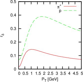
The ansatz in eq. (19) for the local light cone wavefunction with the product of the momentum fractions is motivated by the asymptotic form of the pertubative pion distribution amplitude Fri [03]. This function is very broad and so the quark momenta are strongly smeared around .
The other extreme case is the delta-function approximation of eq. (91) which is already used in the derivation of the CQNS, where the hadron consists of quarks with all having the same momentum . The influence of this strong simplification compared to the realistic light cone wavefunctions is shown in Fig. 8, where I have given the relative deviations for pions and protons.
. 11.2 Effects of the blast wave parameters
. 11.2.1 Baryo-chemical potential
The influence of the baryo-chemical potential on the results is quite neglectable. First of all, it only enters as a factor for each quark in the invariant yield. Second, it drops out of the flow coefficients completely at least for boltzmann statistics. Finally the value of at RHIC and higher energies is much smaller then the temperature (Fig. 6(a)). Therefore the fugacity gives only small corrections.
. 11.2.2 Temperature
The temperature sets the slope of the thermal quark spectrum and also enters the invariant yields. So the temperature is an important parameter, but it varies mainly at low c.m. energies. For it quickly approaches the critical temperature and for RHIC energies and beyond it is essentially constant (Fig. 6(a)). So for the energy range, where recombination can be considered to play an important role, the energy dependence of temperature is not significant.
. 11.2.3 Transverse flow rapidity
The main parameter with the biggest impact on the results is the transverse flow rapidity , since it is expected to show strong variations as the fit from fig. 7 suggests. Although the functional form is very uncertain, the general trend of a rising rapidity can be expected. The exact shape of the dependence is therefore not that important, as long as it fits the value at LHC which is generally expected to be .
The influence of can be studied by looking at the slope of the spectra. The bessel functions (eq. (75)) can be expanded in exponentials with an effective temperature that sets the slope. The inverse temperature can then be found by
| (119) |
For central collisions, a fixed radial coordinate and , this expression can be calculated analytically Sch [93]:
| (120) |
So at high (or ) the effective temperature is blue shifted as
| (121) |
so the slope at high transverse momenta is less steep for a non-zero transverse expansion velocity .


. 11.2.4 Radial profile of the transverse rapidity
The second parameter in the transverse rapidity , beside the mean rapidity , is which models the radial growth in eq. (64) as . In the derivation of the CQNS, I already used the appproximation of a radially constant transverse rapidity i.e. . This is a very unrealistic assumption since there is no pressure gradient in the center and so there should be no expansion. Thus, one expects to be a smoothly rising function of the radial coordinate with a dependence somewhere between square-root and quadratic. Therefore, reasonable values for should be between 0.5 and 2.
The yield and elliptic flow of pions and protons are compared for different values of in Figs. 11 and 12. For the pion yield the modifications are neglectable, but at low the proton yield shows a strong enhancement for higher values of . On the other hand, the elliptic flow decreases with increasing for both particles at low to mid .
The real dependence can be quite non-trivial and can only be studied in dynamical calculations. To have a possibilty to determine a reasonable value, I will compare the results for the yield to experimental data (section . 12.1). The elliptic flow in fact is also very sensitive to the choice of , but it also depends very much on the freeze-out parameters as can be seen in the next sections. Therefore, a fit to data would be too involved and uncertain. That is why I will use , since it is the best fit for the yield and also a reasonable compromise between square-root and quadratic dependence.


. 11.3 Separating flow and non-flow effects
The information about the -dependence of the invariant yield is stored in the fourier coefficients . There are two different mechanisms that generate the azimuthal asymmetric particle yields. So before going into a detailed analysis of the results from and , I will analyse the respective strength of both contributions. The fourier coefficients can be separated in two different contributions:
- •
The flow contribution comes from the asymmetry in the expansion velocity which is parameterized in eq. (62). The asymmetry depends on the initial numerical eccentricity . This is the contribution which results in the CQNS and therefore the more prominent one.
- •
The geometrical contribution comes from the asymmetry of the transverse freeze-out area which depends on the numerical freeze-out eccentricity . Because of its spatial, geometrical origin it is nearly independent of the particle species.
Both effects develop from the the same origin, namely the initial eccentricity in non-central collisions. While the strength of the flow part is fixed by the impact parameter, the geometrical contributions depend on the functional dependence .
Hence, I will first discuss the geometrical and then the flow contributions and after that study the freeze-out eccentricity.
. 11.3.1 Geometrical contributions
To focus on the geometrical contributions, I turn off the flow contributions by setting . Without an initial spatial anisotropy, there is no expansion velocity asymmetry. This normally also means that the freeze-out eccentricity is zero, so I will set it manually to a finite value.
As already explained in section . 7.2 for an elliptic freeze-out, the radial direction is not equal to the one perpendicular to the surface. Thus, we have to investigated the contributions for both models since non should be excluded a priori. Fig. 13 shows and contributions for pions and protons in both scenarios. Due to the geometrical nature, the contributions are nearly equal for pions and protons, so I will not show any calculations for other particle species.
What can be seen directly is that the is equal for both cases, while the switches sign when going from perpendicular (model 1) to radial expansion (model 2). This is the consquence of the transformation behavior of the integration measure derived in section . 7.2. As stated therein, the flow of model 1 is equal to the flow from model 2 with the ellipse rotated by . Reversing this rotation is just switching the x- and y-axis. For , which compares the flow of x- to y-direction, this is equal to changing the sign, but , which compares x- and y-direction to the diagonal direction, is not affected by this rotation.
To distinguish between the models, first one has to predict the orientation of the freeze-out ellipse. Then, by comparing the geometrical together with the flow contributions to experimental data, the correct model can be identified. On the other hand, this means that without the knowledge of the ellipse’ orientation, there is no way to exclude one of the models.
In section . 11.3.3 I will present experimental evidence for the direction of the elongation.

Left: The system expands orthogonal to the surface, which yields a positive (upper curve) and a positive (lower curve).
Right: The system expands radial. The (lower curve) is negative, but with same amplitude, (upper curve) is equal to the other case.
. 11.3.2 Flow contributions
The flow contributions are studied by setting . These contributions are sensitive to the quark content and are the source of the CQNS discussed in sec. . 9.3.1. To simplify the comparison to the geometrical contributions, I also set . The modifcations arising from will be discussed later. Fig. 14 shows the scaled elliptic and hexadecupole flow for different hadrons.
The general trend of the CQNS is clearly visible which is one of the major successes of recombination. Despite the simplifications made in section . 9.3.1, the CQNS is at the heart of the formalism and therefore persists even when calculating with the full space-momentum correlations. Although the very simple scaling law is nice, it should not be taken to far, because the scaling is explicitly broken as discussed in section . 9.4. Most obvious is the additional mass scaling where heavier particles have a smaller and even negative flow coefficient.
The mass scaling between mesons and baryons comes from the sum of the constituent masses as explained in section . 9.4. And the mass scaling among different mesons/baryons comes from the quark flow (Fig. 15) where only the different masses lead to a different elliptic flow. This is also true for . To have an approximate comparison to the scaled elliptic flow, Fig. 14 shows a scaled hexadecupole flow with vs. . The is inspired by an observed constant ratio (for details see sec. . 13.3).

Left: Scaled elliptic flow. Right: Scaled hexadecupole flow.

Left: Elliptic flow. Right: Hexadecupole flow.
. 11.3.3 Relative strength of both contributions
While the flow contributions are fixed by the impact parameter, the geometrical contributions depend on the orientation of the freeze-out ellipse and its eccentricity. To relate the initial and the freeze-out eccentricity, I will use a simple linear ansatz
| (122) |
with the parameter .
To obtain a first approximation, let us compare the results from the previous chapter with a circular freeze-out () to actual data (see Fig. 32 on page 32). As you can see the elliptic flow is generally underpredicted at low . Since only models the high- damping, it has no effect to change it. The only possibility to raise the pion high enough would be to lower the quark mass to a few MeV, which not only is very questionable, but also fails to reproduce the baryons.
Hence, to match the data, one seems to need some additional positive contributions from the geometry. This is achieved by setting . That means the freeze-out eccentricity should be about 70% of the initial eccentricity. This also increases the high region which is compensated by decreasing to .
This is a first hint that is not necessarily zero and needs to be incorporated. This is supported by STAR data Ada [04], where the initial and final eccentricity was calculated via the Glauber model and HBT interferometry. Their results indicate that the elliptic flow cannot quench its initial asymmetry completely.
As discussed in sec. . 8.2, the numerical eccentricity is compared to the glauber eccentricity via
| (123) | ||||
| (124) |

Together with the linear scaling of this relates the initial and the freeze-out eccentricity as
| (125) |
Fig. 16 shows the results of eq. (125) to the STAR calculations, which gives for the best fit case. This good agreement supports the simple linear ansatz in eq. (122) and confirms the first estimate of . But the large systematic errors do not allow a firm conclusion, so is consistent with errors.
This data also clearly indicates a positive which means that the orientation has not changed compared to the initial ellipse and it is still elongated out-of-plane. From what I already said in sec. . 11.3.1, I conclude that the transverse expansion of the system is perpendicular to the surface and drop the surface flow model no. 2 in favor of model 1 (sec. . 7.2).
. 11.4 Correlation between and
So far I only studied the elliptic flow with a constant freeze-out time. To be a bit more general I assume a linear dependence on the radial coordinate as
| (126) |
For a given mean freeze-out time it follows
| (127) |
With a constant freeze-out time is recovered. This is a quite simple ansatz, but it suffices to study a general dependence.
The dependence of the yield on is shown in Fig. 17 for different hadrons. The relative deviations is similiar for mesons and baryons and approximately independent of with about -0.2 for and 0.2 for .
The deviations of the elliptic flow for different are shown in Fig. 18 for an elliptic freeze-out with . For a circular freeze-out the deviations are neglectable. So non-zero has the largest effects on at low . This behaviour is similar for the hexadecupole flow.


. 12 Transverse momentum spectra
In this section I show hadron production for Au+Au collisions at from recombination. For the LHC predictions of Pb+Pb collisions at I will use the same nuclear size , since the radius only enters an overall factor and there is no data yet available to compare to.
. 12.1 Yields

Fig. 19 shows the transverse momentum spectra of light and strange hadrons compared to data from PHENIX Chu [03] and STAR Abe [06], Min [08], Abe [07], Ada07a [] for different centralities. In the mid range, the results agree with the data. But below and especally below , the data is significantly underpredicted for hadrons with light quark content. This is due to the energy violation in the recombination formalism and also the contributions from resonance decay are not incorporated. For hadrons with only strange quark content, namely and , the predictions are in good agreement even down to very low , since for the massive particles the energy violation is not that strong and the contributions from resonance decay are minor. The black lines correspond to LHC predictions for an impact parameter of .
Fig. 20 shows the transverse momentum spectrum of charged hadrons compared to data from STAR Ada [03] for different values of , the parameter for the radial profile of the transverse rapidity. While the results are equal at low , they differ for and the best fit is achieved for about . But the large deviations from the data at low do not allow for a firm conclusion on that parameter. Another analysis is given in sec. . 13.3.2, where I study the dependence of the flow ratios on this parameter. For now I will use . The other parameters are and as discussed in the previous sections. The negative gives a constant factor of about 1.2 while the freeze-out eccentricity does not affect the transverse momentum spectra, since it is chosen to preserve the total transverse freeze-out area.

. 12.2 Mean transverse momentum

Fig. 21 shows the mean transverse momentum as a function of the hadron mass in the left panel. The results for RHIC (red points) are compared to data from STAR Abe08a [] (blue points). At low hadron mass, namely for pions and kaons, the results for the mean overestimate the data, since the low yield is underestimated as shown in the previous paragraph. For protons and heavier hadrons, the deviations for the yield are smaller and therefore the predicitions of the mean are in much better agreement.
Additionally, in the right panel I show the mean transverse velocity at midrapidity calculated from the mean . As one can see, this quantity softens the deviations for the light mesons. For masses of about the velocity approaches the value of the mean transverse expansion (black lines) at RHIC. Similiar the predictions for the LHC (green points) approach .
The figure also depicts calculations from the equipartition theorem (red/green lines), which states
| (128) |
with the temperature and the Boltzmann constant (which is equal to 1 in natural units). Using the energy from eq. (68) in the local rest frame, this leads to
| (129) | ||||
| (130) | ||||
These equations are coupled via so they need to be solved numerically.
Interestingly, the values for hadron masses above are larger then the results from recombination, if one uses the same temperature and transverse velocity or respectively . Therefore, the mean velocity reaches these “limiting” values much later. When using and as fit parameters, the equipartition theorem reproduces the recombination results for , for RHIC and for LHC.
. 12.3 Hadron ratios

The large proton/pion ratio at mid was one of the puzzles that fragmentation failed to describe and thus, it is one of the motivations for studying recombination. So, Fig. 22 shows the ratios of the invariant yields from different hadrons compared to data from PHENIX Adl [03] and STAR Lon [04], Min [08]. The low region is mainly overestimated which can be attributed to the failed description of the spectra at low , due to the energy violation. The mid results are between a mediocre and good agreement, apart from the to ratio which is about a factor of 2 smaller. The main point is the prediction of the large proton to pion ratio of about 1. The high region is badly predicted and would require the combined treatment of recombination and fragmentation Fri [03].
The black lines correspond to LHC predictions, but with the same strange fugacity which would have to be extracted from fits and can be expected to be larger.
. 13 Flow coefficients and
In this section, I study the elliptic and hexadecupole flow at RHIC and LHC. I will start with the eccentricity dependence of the mean flow coefficients. The findings will motivate the investigation of the flow ratio which will support the findings in sec. . 11.3.3 about the freeze-out eccentricity.
This ratio also gives the opportunity to study a correlation and the radial profile of the transverse expansion rapidity. The obtained values for the corresponding parameters in the sections . 13.3.1 and . 13.3.2 will be used in the comparison to experimental data of the differential flow coefficients.
. 13.1 Mean flow coefficients
The mean elliptic or hexadecupole flow at midrapidity is the integrated average folded by the transverse momentum distribution:
| (131) |
. 13.2 Eccentricity dependence
The strength of the flow coefficients depends on the impact parameter or respectively the eccentricity. To study the dependence, I will compare the mean, -integrated flow to the eccentricity . Looking at equation eq. (62), one expects the mean to scale mainly linear with and to have a larger quadratic contribution.
Therefore, the calculations are fitted by and shown in Figs. 23 and 24. The fit values support the expected behaviour and can be found in Tab. 1.

Upper: Mean elliptic flow. Lower: Mean hexadecupole flow.

| 1.58e-01 | 1.28e-01 | 1.02e-01 | 1.37e-01 | 1.15e-01 | 7.57e-02 | |
| 1.04e-01 | 7.95e-02 | 6.39e-02 | 7.26e-02 | 7.20e-02 | 8.06e-02 | |
| 3.05e-01 | 2.72e-01 | 2.47e-01 | 2.94e-01 | 2.80e-01 | 2.63e-01 | |
| -1.17e-01 | -1.23e-01 | -1.25e-01 | -1.43e-01 | -1.40e-01 | -1.31e-01 | |
| -4.92e-03 | -3.13e-03 | -1.75e-03 | -2.00e-03 | -1.21e-03 | -7.62e-05 | |
| 6.11e-02 | 4.36e-02 | 2.86e-02 | 4.00e-02 | 2.65e-02 | 2.06e-03 | |
| 6.67e-03 | 7.05e-03 | 7.08e-03 | 1.08e-02 | 1.05e-02 | 9.36e-03 | |
| 8.43e-02 | 6.85e-02 | 5.61e-02 | 8.02e-02 | 7.31e-02 | 6.33e-02 |
. 13.2.1 Fluctuations
For a fixed impact parameter, the eccentricity is expected to fluctuate Vol [08], Bro [07]. Since the flow components scales with powers of , the fluctuations in the -integrated can be related to the eccentricity fluctuations. To study these fluctuations, I take the fits from table 1, where I used
| (132) |
I assume a gaussian distribution of the eccentricity around the mean expected eccentricity as
| (133) |
with a width that generally can depend on the mean eccentricity. The mean of the elliptic flow distribution can then be calculated as
| (134) |
and the fluctuations are
| (135) |
where is the -integrated mean and denotes the fluctuation mean.
The relative fluctuations for a purely linear dependence () simplify to
| (136) |
For a purely quadratic dependence () the relative fluctuations scale with as
| (137) |
Looking at the fit values in table 1, the quadratic contributions for the elliptic flow are small compared to the linear ones () and vice versa for the hexadecupole flow ().
The relative fluctuations of the eccentricity are predicted to be approximately constant with Dre [07], Alv [07], Sor [07]. As can be seen in Figs. 25 and 26, the relative fluctuations of the elliptic flow is almost independent of the particle type and also comparable to the fluctuations of the eccentricity as eq. 136 suggests. On the other hand the relative hexadecupole fluctuations are much smaller and approch the value from eq. 137 for large . The divergence of at low is due to the negative fit value of , so that the denominator becomes zero at a finite .


. 13.3 Flow ratio
As was shown in the last section, for a circular freeze-out the different flow coefficients will scale with the eccentricity mainly as . Therefore ratios of these coefficients are an interesting probe to study, since the flow contributions will be insensitive to the initial geometry. The geometrical contributions from an elliptic freeze-out on the other hand can have great influence on these ratios. So they offer the possibility to verify the statements about the freeze-out eccentricity. One can also take a closer look on the influence of a correlation () and the radial profile of transverse expansion ().

I will focus on the ratio , that I already discussed shortly in framework of the CQNS (sec. . 9.3.2). For a quick approximation of the value for the quarks I compare the prefactors from the transverse rapidity (eq. (62)): and , which yields . This will turn out to be too small. Inserting a more realistic value of 1 in the scaling law from section . 9.3.2 gives constant values of
| (138) |
and
| (139) |
So the simple cqns formulas suggest a ratio around 0.7. But these values are much smaller than the experimental values from STAR Bai [07] (with ) and PHENIX Hua [08] (with ). Also the full calculations give a similiar value of about 0.7 from mid to high . That indicates that we have to consider contributions from geometrical effects.
Fig. 27 shows the flow ratio for charged hadrons. The lines correspond to different percentages of the freeze-out eccentricity to the initial one. The left figure corresponds to an impact parameter of , the right one to . The good agreement between both supports the predicted independence from the eccentricity.
At low the ratio is much greater than for all percentages of the freeze-out eccentricity. At mid the effect of an elliptic freeze-out is most clearly visible. While for the ratio is about 0.6, it rises to about for . The three curves with and , which are the estimates from sec. . 11.3.3 within errors, only differ at low . For these three values the ratio is in the range of the experimental data. So to compare the results to experimental data, I will take the best fit case of and in the next two paragraphs I look at the dependence on two other parameters, namely and .
. 13.3.1 Influence of a correlation
This is dependence is studied by varying the parameter (see section . 11.4). Therefore I fix , which means a linear growth if the transverse rapidity. The upper panel in Fig. 28 shows the ratio for charged hadrons at for compared to data from STAR Bai [07], Pos [04]. A constant freeze-out time, i.e , seems to give the best agreement. This different to the lower panel with at for pions, protons and kaons, where at high the value is independent of , but the predictions for at low overestimate the data. A very good agreement at least for the mesons can be found with . A (negatively) larger for baryons could increase the agreement at low , but the very sharp drop of the proton ratio can not be accounted for. And it also would enhance the discrepancy to the charged hadron data from STAR.
A negative describes a fireball, where the outer particles freeze-out earlier ( than the inner ones (). With and a mean freeze-out time , this corresponds to and . The data does not allow to draw a firm conclusion about the value of , since it also could (or even should) depend on the particle species or on their in-medium cross sections respectively. But the case of a large positive , where the , can be discarded.


. 13.3.2 Influence of the radial rapidity profile
The radial profile of the transverse rapidity is set by the parameter (see section . 11.2.4). So this time I use a constant .
The behaviour for different is similiar to the previous paragraph. At high all three curves give the same result and only at low the values are modified. The data on charged hadrons (Fig. 29, upper panel) is best reproduced with (and ) as in the previous paragraph. The data from PHENIX on pions and kaons seems to favour a smaller of about 0.5, while proton data at low points to , where still gives a large overestimation.
So generally both parameters can be used to fine tune the ratio and this would preclude a determination of these parameters from this observable. But there are two reason to fix at a value of and use as a free parameter:
- •
The low pion data could be explained by a lower value of for baryons. A larger value of on the other hand is not only unreasonable, but also largely fails to predict the meson data. And since is a blast-wave parameter is would be inconsistent to let it depend on the particle species.
- •
The outer particles in the shell of the fireball suffer less collisions, since they can expand into the vacuum, and therefore one expects them to freeze-out earlier than the particles in the inner fireball. From that, one would expect a negative , which is supported by hydrodynamical calculations Kis [06], Cho [06].


. 13.4 Differential flow
In this section I will show differential elliptic and hexadecupole flow compared to data from RHIC. I will use the parameters as extracted from the previous sections as , and if not specified otherwise. To show the relevance of these parameters, Fig. 30 compares the elliptic flow of charged hadrons with an impact parameter of for three different freeze-out scenarios: circular freeze-out with (blue line), elliptic freeze-out with (green line) and elliptic freeze-out with , (red line). Again, a circular freeze-out can be safely discarded. An elliptic freeze-out with a radial decrease of the freeze-out time () is the best description of the STAR data Tan [04] and only gives a slight underestimation at low . The data points correspond to the event plane (squares) and two-particle cumulant method (circles) for the determination of the elliptic flow.


Fig. 31 compares the differential elliptic flow of identified hadrons to data from RHIC from different centralities. The red data points are from STAR with a centrality of 40-80% and the green ones from PHENIX with 20-60% centrality. They are compared to an impact parameter of (red lines) and (green lines) respectively.
The agreement is quite good. While the behaviour at high changes with the phenomenological parameter , the precise predictions at mid and low confirm the relevance of the parameter . To show that a large freeze-out eccentricity of about 70% of the initial one is not only need for the flow ratio from the previous section, but also for the differential elliptic flow, Fig. 32 gives the same comparison for and .
So for a circular freeze-out the low and mid range is generally underpredicted for all hadrons and the high region only agrees, because of a larger . As can be seen, a remaining freeze-out eccentricity can not be neglected.

The predictions for LHC (black lines) are also shown. A first striking observation is that the values are generally smaller. A similar pattern was also observed within a parton transport approach, if the viscosity was set to the ADS/CFT limit Mol [07]. It seems as the elliptic flow reaches a maximum somewhere between these two center of mass energies which is due to the increased transverse expansion velocity from (RHIC) to (LHC). I have already shown this strong dependence on in section . 11.2.3. At low the elliptic flow becomes even negative for (multi-)strange particles which will be exploited in the following sections . 13.6 and . 13.8. A discussion about the negative flow then follows in section . 13.9.
For the fourth fourier coefficient , experimental data is rare up to now. Fig. 33 shows the hexadecupole flow of different hadrons for an elliptic freeze-out compared to the available data from PHENIX Hua [08]. The pion results agree very well with the data while the kaon and proton data is slightly overestimated at low . Also the predictions for the LHC (blue lines) are shown.

. 13.5 Deuteron flow
Due to their small binding energy, deuterons are expected not to survive the early phase, but to be produced by proton-neutron coalescence at freeze-out Sch [97], Nys [04]. Thus, the invariant yield can be written as
| (140) |
with and a coalescence parameter which will depend on the freeze-out volume. Hence, the elliptic flow is related by
| (141) |
But by inserting the CQNS for the proton elliptic flow, the expected scaling of the deuteron flow with the quark flow is obtained:
| (142) |
Thus, the general behaviour of the deuteron elliptic flow seems to be independent of the production process: (after the freeze-out of and ) or (at hadronization).
Fig. 34 compares both cases with realistic calculations at to data from PHENIX Afa [07] (cent. 20-60%) and STAR Liu [07] (minimum bias). The red line corresponds to the scenario of 6 recombining quarks at hadronization which agrees very well with the data. Only at very low , it does not follow the STAR data of a slightly negative . The green line depicts the scaled proton elliptic flow which does not give the same results but follows the same trend as expected. It overestimates the data which may be due to the “delta-shaped wavefunction” approximation . So, while the study of the transverse momentum spectra requires a dynamical treatment with hadronic degrees of freedom, the elliptic flow can be described by quark recombination and thus follows the CQNS. Additionally, the black line shows the prediction for the LHC for the quark recombination scenario.

. 13.6 Heavy quark flow
A large elliptic flow implies, from a hydrodynamical point of view, a rapid thermalization of the fireball and a strong collective flow created at the QGP stage. This assumption is well established and the large flow of light quarks is reflected in the good agreement with the data. Heavy quarks on the other side have a much larger mass then the light quarks and therefore it is an open question, if charm or even bottom quarks participate in the collective expansion.
The recently published data on from PHENIX offer the possibility to investigate whether also the charm quark does locally equilibrate and therefore follows the flow of the light quarks. The most prominent feature of this preliminary data, despite its large errors, is the negative value at . Within the CQNS this implies also a negative elliptic flow for the charm quark. Since the multistrange also shows a slightly negative for a mean transverse expansion velocity of , the much heavier charm quark can be expected to show an even more pronounced behaviour, when assuming a similar transverse expansion.

Left: Comparison for increasing mean expansion velocities from top to bottom with and . The lowest line (black) corresponds to and .
Right: Comparison for different with and .
The elliptic flow for is depicted in Fig. 35 together with the data from PHENIX Sil [08]. The left panel is calculated with the parameter and shows different expansion velocities and the right panel compares for different values of .
Looking at the left panel, the lines from top to bottom correspond to and with , while the last line (black) is for from a circular freeze-out (). So a large charm flow that is equal to the light quark flow seems to produce large out-of plane elliptic flow (, black line), but this is compensated by the positive geometrical contributions from the elliptic freeze-out. Nevertheless, small transverse expansion velocities seem to be discarded due to the large positive at , while a thermalized charm with is at least consistent with zero flow at . I would like to mention that the discussion from Kri [07] is for a circular freeze-out only, since we had employed only the simpified equations from Fri [03].
From the flow ratio section I predicted a negative . This delayed freeze-out of the particles in the inner fireball can be explained by in-medium rescattering. But the is expected to have a low cross-section, i.e. it can escape the system quite undisturbed. So the will freeze-out early, while the system is still expanding. Therefore one could assume a zero or even positive . This is depicted in the right panel of Fig. 35 for a mean expansion velocity , where the data clearly seems to favor a positive (blue line).
The large errorbars do not allow to draw any firm conclusions, but I want to state that the data is consistent within errors with a charm quark flow of equal to the light quarks and a positive (). At least one can extract a lower bound on the expansion velocity of about . So if more precise data will still support the negative , I conclude from this observation that charm quarks reach a substantial amount of local kinetic equilibration.
Another possibility is to study -meson elliptic flow. There, the positive light quark will compete with the negative one from the charm quark. So far, there is no data on -meson elliptic flow available, but in the near future the Heavy Flavor Tracker (HFT) from STAR will close this gap. Preliminary, one could compare to data of electrons from heavy flavor decay. This is no direct probe of the charm flow, since there will be contributions from -mesons and the decay kinematics might smear out the charm flow signal. However, calculations within transport theory Gre [04] predict the -meson elliptic flow to be similiar to the heavy-electron .

Fig. 36 compares the electron elliptic flow data from PHENIX Ada07b [] to for different charm transverse velocities (lines, top to bottom) with and . The elliptic flow agrees with the electron data at low , but does not allow for a distinction between the different transverse velocities. While the data follows the curve for a below , above it is better predicted by a large expansion velocity of . But at high , the of the electrons is generally about a factor of 2 smaller then that of the . That might be due to an early onset of the fragmentation regime for the charm. Again, there is no clear conclusion, but the data does not seem to contradict a large charm transverse velocity, which is comparable to the light quark velocity of , as far as the heavy electron can be compared to the elliptic flow.
As a finally comparison, Fig. 37 shows the elliptic flow for charm and bottom mesons at RHIC (left) and LHC (right) for and .

. 13.7 Centrality dependence
Fig. 38 shows the mean elliptic flow of charged hadrons as a function of the centrality. The left panel is for an elliptic freeze-out and the right for a circular one. Although the differential shows very good agreement with the data as shown above, the results for (left panel, red line) generally overestimate the data from STAR Abe08b []. This is due to the yield at low , which is to small because of energy violation and the absence of resonance feed-down as discussed in section . 12.1. Therefore the mean weighted with the yield favors larger values. I account for that by scaling the results with a constant factor of (green line), so that they are in agreement with the data for the central and mid-central collisions, but for peripheral collisions the data is still overestimated. This is due to the used eccentricity (eq. (60)), which follows the glauber eccentricity for central and mid-central collisions, but gives wrong results for peripheral collisions (Fig. 4).
The mean from a circular freeze-out fails to describe the data and underestimates it as expected. Only to have a comparison between both cases, I will scale the mean elliptic flow value for by a constant factor of 1.3 (right panel, green line) so that it fits the data for central to mid-central collisions. In the next section I will use both factors implicitly.

Left: from an elliptic freeze-out. Right: from a circular freeze-out.
Due to the lack of similiar data for the hexadecupole flow, I compare the results to of charged hadrons for different centrality classes from PHENIX Iss [08] in Fig. 39. The agreement with the data is quite good within the uncertainty of relation between the impact parameter and the centrality. But an underestimation of the mean for peripheral collisions can be expect similiar to the mean elliptic flow.

. 13.8 dependence
The effect of a negative elliptic flow at low at LHC will be visible even for hadrons with light quark content, like protons as shown in Fig. 31. Therefore, it is interesting to look at the mean elliptic flow as a function of the center of mass energy . To compare the results from an elliptic and circular freeze-out, Fig. 41 uses the correction factors from the previous section.
The shown value for LHC in Fig. 41 is just a linear interpolation, but the general expectation in the heavy ion community is an monotonic increase from RHIC energies to LHC and beyond, or at least a saturation at some finite value. In this framework, the value of depends on the interplay of the strength of the negative and the increasing mean , since . But as can be seen in Fig. 41, the increase in the mean does not seem to compensate the increasing effect of the negative at low . Depending on the used freeze-out eccentricity, the maximum of the mean elliptic flow is reached somewhere between RHIC and LHC energies, while a larger eccentricity (a larger ) delays the extremal point to higher c.m. energies. For the best fit case of the value at LHC is maximal and then starts to drop; for a circular freeze-out with it would have already reached its maximum at RHIC. This may mean that even if this striking prediction is correct, there will be no clear sign of a decreasing mean elliptic flow for charged hadrons at LHC. But the mean elliptic and hexadecupole flow of identified hadrons can be a much better probe. As can be seen in Fig. 40, the and of pions, ’s and protons reach their maximum at LHC energies. And while the of the and only indicate a small decrease, the of these heavy hadrons will show a visible drop when going from (RHIC) to (LHC).


A rather critical assumption in this context is the applicability of the recombination approach for the elliptic flow for small transverse momenta on the order of . I want to emphasise that the result of the decreasing mean elliptic flow at LHC is not affected by the validity of this assumption, because and in LHC regime. However, to show the robustness of the prediction Fig. 42 depicts the elliptic flow at a fixed as a function of with an impact parameter . With the exhibits the same drop as the mean elliptic flow from Fig. 41. The data points are taken from Adl [05] with a centrality of 13-26%. They confirm the observation of an elliptic flow saturation at .

As can be seen in Fig. 43, the mean hexadecupole flow shows a similar dependence on the center of mass energy. In the case of an elliptic freeze-out (red line), the increase from RHIC to LHC is much more pronounced as for the elliptic flow, but also the drop beyond its maximum at LHC is much stronger. In the case of a circular freeze-out (green line), the predicted value is already negative at LHC.

Since both flow coefficients show a similiar behaviour as a function of , I will also take a look at the ratio . Fig. 44 shows this ratio for charged hadrons as a function of the center of mass energy at an impact parameter of (solid lines) and (dashed lines). The results for both impact parameters are nearly equal, hence this mean ratio is also independent of the centrality, like the dependent ratio in section . 13.3. For a circular freeze-out (green lines), the ratio is approximately constant between 1.3-1.5 up to RHIC energies and is steeply dropping when going to LHC while for an elliptic freeze-out (red lines), it is constant at about 1.3 up to LHC energies.

. 13.9 Analyzing the negative elliptic flow
At low center of mass energies, the elliptic flow is generally negative, since the spectators in a non-central collision are blocking the in-plane flow. This behaviour, also known as anti-flow, is not observed at high bombarding energies, since the nuclei are strongly lorentz-contracted. Then the flow asymmetry only depend on the spatial asymmetry as discussed.
The predicted negative elliptic flow at low transverse momenta is different to anti-flow. It has also been found in previous exploratory studies and seem to be a general feature of the blast-wave like flow profile at high transverse velocities Vol [97], Huo [01], Vol [02], Ret [04], Pra [05]. One might argue that this is an artefact of the blast-wave peak and will not survive in more realistic calculations, however, also transport simulations indicate slightly negative values for heavy particles at very low Ble [02] and the AMPT model predicts a negative at least for heavy charm and bottom quarks Ko [07]. Thus, the qualitative behaviour of a negative is a well-known observation. The magnitude, however, of this effect and the particle species affected by it depend on the mass, the amount of transverse flow and the decoupling hyper-surface of this individual particle species. So the surprising observation of a drop in the mean elliptic flow at LHC and an even negative value beyond is not the existence of the elliptic ’anti-flow’ but the quantitative strength and influence on the light quark sector of this effect at LHC.
To obtain an analytic expression which explains the negative is to consider only the in-plane () and out-of-plane () directions (similar to the analysis performed in Huo [01]). The integration breaks down (eq. (86)) and the elliptic flow is then given by
| (143) |
For the argument of the Bessel functions (see eq. (76)) goes to zero and becomes constant with and . Therefore they are independent of the angle. This leads to
| (144) |
Since is a monotonically decreasing function, the numerator and thus the elliptic flow is negative (for some small transverse momenta). The specific values depend on the mass, the mean flow rapidity and the temperature. For increasing mass (e.g. charmed mesons) or increasing transverse flow rapidity (e.g. LHC and beyond) or decreasing temperature, the elliptic flow will become more negative.
Another way to understand this effect in more detail one could look directly at the thermal quark-spectrum with the energy (eq. (68))
| (145) |
For simplicity let us look at midrapidity () and for high the spectrum is very low, so I consider the region around . For high c.m.-energies, when the source is highly boosted transversally, the particles will mainly be emitted in the direction in which the fireball flies, so one can simplify even more and set . Because in this case there is no longitudinal momentum I can replace the momentum with , the transverse rapidity of the parton, as
| (146) | ||||
| (147) |
So the energy of the quark in the transverse moving source is given by
| (148) |
For a fixed quark rapidity (low ) the energy of the quarks emitted in-plane is higher than the energy of quarks emitted out-of-plane. With the thermal spectrum more energy means less particles, therefore a negative . At one would expect the zero-crossing, and above a positive .
Chapter Conclusion
When studying the elementary building blocks of our universe throughout history, higher and higher energies were needed to resolve the ever smaller structures. Now, physicists are searching for the so-called Quark Gluon Plasma (QGP), a state of matter where the quarks are not confined inside the hadrons but free particles. The transition to this new phase of the strongly interaction matter is probed within Heavy Ion Collisions (HIC) at the Relativistic Heavy Ion Collider (RHIC) and soon with the Large Hadron Collider (LHC).
One major problem in this context is the question if we have created a QGP in a collision, since the hadronization happens on very small timescales, so that only the hadrons from freeze-out can be measured. But also a dynamical description within QCD, of the collision in general and the hadronization process in particular, is not expected to be achieved in the near future. Thus, we depend on phenomenological models.
The description via pQCD with the use of measured, parameterized fragmentation functions is very successful for proton-proton collisions, but in HIC with a dense phase space this approach is only applicable at high . With the first results from RHIC which pQCD failed to describe, a phenomenological model named recombination became popular.
One of the most promising observables to study the creation of a QGP is the elliptic flow which is the second fourier coefficient of the invariant yield. It measures the azimuthal asymmetry of the transverse momentum which orginates from the spatial asymmetry in non-central collisions. Since it shows a self-quenching behaviour, the measured elliptic flow of the hadrons is mainly sensitive to the initial stage of the collision. Therefore, it would depend on the partonic elliptic flow from the QGP.
The success of recombination is mainly based on the prediction of a universal scaling law of the elliptic flow which connects the hadron elliptic flow directly with the quark elliptic flow. This predicted constituent quark number scaling (CQNS) is experimentally well observed and the results can describe the data very accurately at low and mid . While the qualitative behaviour of the particle species dependence of follows the CQNS law of recombination, the quantitative results depend on the two additional “ingredients”: the quark density distribution and the hadronization/freeze-out hypersurface.
In this thesis I have shown that these two additionial inputs have strong influence on the flow coefficients. For the quark density distribution I employed the blast-wave model which is inspired by hydrodynamics. It describes a transversally expanding, locally thermalised fireball. A simple geometrical argument to parameterize the pressure gradient suffices to describe not only the elliptic flow but also the next coefficient . A result of the blast-wave flow profile is the observed mass scaling of the elliptic flow and especally a negative flow coefficient at low for massive particles and/or high center of mass energies. Such a negative value can also been seen in the preliminary elliptic flow data from PHENIX which seems to support the predictions. The most striking prediction of recombination in this framework using the blast-wave model is then a dropping mean at or beyond LHC energies.
The hadronization occurs within a 3-dimensional, time-dependent volume and coincides with the kinematic freeze-out, since there is no hadronic scattering phase. The detailed study of this freeze-out hypersurface would require a dynamical treatment. But to identify a general influence on the spectra, this analytical approach is sufficient, since also in hydrodynamics the process of particle freeze-out is a highly non-trivial problem. As I have shown, a remaining spatial eccentricity at freeze-out and a radial dependence of the freeze-out time have the greatest impact on the flow coefficients, and especally on their ratio . While a simple circular freeze-out underestimates this flow ratio by a factor of 2, an elliptic freeze-out introduces additional contributions to both flow coefficients and can describe the experimental data very well. The behaviour of the flow ratio at low is then affected by the radial dependence of the freeze-out time.
The presented results in this thesis indicate that recombination is the dominant mechanism for hadron production at mid while the flow coefficients and their constituent quark number scaling are a strong sign for an early partonic stage of the collision. Despite its phenomenological nature, this analytical approach to recombination as the hadronization mechanism in HIC, together with an appropriate quark density and freeze-out hypersurface, describes not only the qualitative constituent quark number scaling of the experimental data, but also the quantitative mass scaling of the elliptic and hexadecupole flow and the large ratio of these coefficients with great detail. Based on this good agreements, the striking predicitions for the LHC should be considered in more detail within a dynamical model.
References
- Abe [06] Abelev, B. I. et al.: Identified baryon and meson distributions at large transverse momenta from Au + Au collisions at s(NN)**(1/2) = 200-GeV. Phys. Rev. Lett. (2006), Bd. 97:S. 152301
- Abe [07] Abelev, B. I. et al.: Partonic flow and Phi-meson production in Au + Au collisions at s(NN)**(1/2) = 200-GeV. Phys. Rev. Lett. (2007), Bd. 99:S. 112301
- [3] Abelev, : B. I.: Measurements of meson production in relativistic heavy-ion collisions at RHIC (2008)
- [4] Abelev, B. I. et al.: Centrality dependence of charged hadron and strange hadron elliptic flow from = 200 GeV Au+Au collisions. Phys. Rev. (2008), Bd. C77:S. 054901
- Ada [03] Adams, John et al.: Transverse momentum and collision energy dependence of high p(T) hadron suppression in Au + Au collisions at ultrarelativistic energies. Phys. Rev. Lett. (2003), Bd. 91:S. 172302
- Ada [04] Adams, John et al.: Azimuthally sensitive HBT in Au + Au collisions at s(NN)**(1/2) = 200-GeV. Phys. Rev. Lett. (2004), Bd. 93:S. 012301
- [7] Adams, J. et al.: Scaling Properties of Hyperon Production in Au+Au Collisions at = 200 GeV. Phys. Rev. Lett. (2007), Bd. 98:S. 062301
- [8] Adare, A. et al.: Energy Loss and Flow of Heavy Quarks in Au+Au Collisions at = 200 GeV. Phys. Rev. Lett. (2007), Bd. 98:S. 172301
- Adl [03] Adler, Stephen Scott et al.: Scaling properties of proton and anti-proton production in s(NN)**(1/2) = 200-GeV Au + Au collisions. Phys. Rev. Lett. (2003), Bd. 91:S. 172301
- Adl [05] Adler, Stephen Scott et al.: Saturation of azimuthal anisotropy in Au + Au collisions at s(NN)**(1/2) = 62-GeV - 200-GeV. Phys. Rev. Lett. (2005), Bd. 94:S. 232302
- Afa [07] Afanasiev, S. et al.: Elliptic flow for mesons and (anti)deuterons in Au+Au collisions at = 200 GeV. Phys. Rev. Lett. (2007), Bd. 99:S. 052301
- Alv [07] Alver, B. et al.: Elliptic flow fluctuations in Au+Au collisions at 200 GeV (2007)
- Bai [07] Bai, Yuting: The anisotropic flow coefficients v(2) and v(4) in Au + Au collisions at RHIC. J. Phys. (2007), Bd. G34:S. S903–906
- Bas [98] Bass, S. A. et al.: Microscopic models for ultrarelativistic heavy ion collisions. Prog. Part. Nucl. Phys. (1998), Bd. 41:S. 255–369
- Bas [99] Bass, S. A.; Gyulassy, M.; Stoecker, Horst und Greiner, W.: Signatures of quark-gluon-plasma formation in high energy heavy-ion collisions: A critical review. J. Phys. (1999), Bd. G25:S. R1–R57
- Bjo [83] Bjorken, J. D.: Highly Relativistic Nucleus-Nucleus Collisions: The Central Rapidity Region. Phys. Rev. (1983), Bd. D27:S. 140–151
- Ble [99] Bleicher, M. et al.: Relativistic hadron hadron collisions in the ultra- relativistic quantum molecular dynamics model. J. Phys. (1999), Bd. G25:S. 1859–1896
- Ble [02] Bleicher, Marcus und Stoecker, Horst: Anisotropic flow in ultra-relativistic heavy ion collisions. Phys. Lett. (2002), Bd. B526:S. 309–314
- BM [03] Braun-Munzinger, Peter; Redlich, Krzysztof und Stachel, Johanna: Particle production in heavy ion collisions (2003)
- Bor [08] Borghini, Nicolas und Wiedemann, Urs Achim: Predictions for the LHC heavy ion programme. J. Phys. (2008), Bd. G35:S. 023001
- Bro [02] Broniowski, Wojciech und Florkowski, Wojciech: Geometric relation between centrality and the impact parameter in relativistic heavy ion collisions. Phys. Rev. (2002), Bd. C65:S. 024905
- Bro [07] Broniowski, Wojciech; Bozek, Piotr und Rybczynski, Maciej: Fluctuating initial conditions in heavy-ion collisions from the Glauber approach. Phys. Rev. (2007), Bd. C76:S. 054905
- CBM [07] CBM, collaboration: The CBM Experiment: Introduction (2007), URL http://www.gsi.de/fair/experiments/CBM/1intro.html
- Cho [74] Chodos, A.; Jaffe, R. L.; Johnson, K.; Thorn, Charles B. und Weisskopf, V. F.: A New Extended Model of Hadrons. Phys. Rev. (1974), Bd. D9:S. 3471–3495
- Cho [75] Chodos, Alan und Thorn, Charles B.: Chiral Hedgehogs in the Bag Theory. Phys. Rev. (1975), Bd. D12:S. 2733
- Cho [06] Chojnacki, Mikolaj und Florkowski, Wojciech: Characteristic form of boost-invariant and cylindrically non-symmetric hydrodynamic equations. Phys. Rev. (2006), Bd. C74:S. 034905
- Chu [03] Chujo, T.: Results on identified hadrons from the PHENIX experiment at RHIC. Nucl. Phys. (2003), Bd. A715:S. 151–160
- Cle [06] Cleymans, J.; Wheaton, S.; Oeschler, H. und Redlich, K.: Comparison of chemical freeze-out criteria in heavy-ion collisions. PoS (2006), Bd. CPOD2006:S. 035
- Coo [74] Cooper, Fred und Frye, Graham: Comment on the Single Particle Distribution in the Hydrodynamic and Statistical Thermodynamic Models of Multiparticle Production. Phys. Rev. (1974), Bd. D10:S. 186
- dF [06] de Forcrand, Philippe und Philipsen, Owe: Towards the QCD phase diagram. PoS (2006), Bd. LAT2006:S. 130
- Dre [07] Drescher, Hans-Joachim und Nara, Yasushi: Eccentricity fluctuations from the Color Glass Condensate at RHIC and LHC. Phys. Rev. (2007), Bd. C76:S. 041903
- Flo [04] Florkowski, Wojciech und Broniowski, Wojciech: Hydro-inspired parameterizations of freeze-out in relativistic heavy-ion collisions. Acta Phys. Polon. (2004), Bd. B35:S. 2895–2910
- Fod [02] Fodor, Z. und Katz, S. D.: Lattice determination of the critical point of QCD at finite T and mu. JHEP (2002), Bd. 03:S. 014
- Fri [03] Fries, R. J.; Muller, Berndt; Nonaka, C. und Bass, S. A.: Hadron production in heavy ion collisions: Fragmentation and recombination from a dense parton phase. Phys. Rev. (2003), Bd. C68:S. 044902
- Fri [04] Fries, R. J. und Muller, Berndt: Heavy ions at LHC: Theoretical issues. Eur. Phys. J. (2004), Bd. C34:S. s279–s285
- Gas [81] Gasiorowicz, Stephen und Rosner, Jonathan L.: HADRON SPECTRA AND QUARKS. Am. J. Phys. (1981), Bd. 49:S. 954
- Gla [70] Glauber, R. J. und Matthiae, G.: High-energy scattering of protons by nuclei. Nucl. Phys. (1970), Bd. B21:S. 135–157
- Gre [04] Greco, V.; Ko, C. M. und Rapp, R.: Quark coalescence for charmed mesons in ultrarelativistic heavy-ion collisions. Phys. Lett. (2004), Bd. B595:S. 202–208
- Hir [06] Hirano, Tetsufumi; Heinz, Ulrich W.; Kharzeev, Dmitri; Lacey, Roy und Nara, Yasushi: Hadronic dissipative effects on elliptic flow in ultrarelativistic heavy-ion collisions. Phys. Lett. (2006), Bd. B636:S. 299–304
- Hua [08] Huang, S.: Measurements of high identified particles and in GeV Au+Au collisions by PHENIX. J. Phys. (2008), Bd. G35:S. 104105
- Huo [01] Huovinen, P.; Kolb, P. F.; Heinz, Ulrich W.; Ruuskanen, P. V. und Voloshin, S. A.: Radial and elliptic flow at RHIC: Further predictions. Phys. Lett. (2001), Bd. B503:S. 58–64
- Iss [08] Issah, Michael: System size and beam energy dependence of azimuthal anisotropy from PHENIX. J. Phys. (2008), Bd. G35:S. 104103
- Jac [00] Jacobs, Peter und Cooper, Glenn: Spatial Distribution of Initial Interactions in High Energy Collisions of Heavy Nuclei (2000)
- Kis [06] Kisiel, Adam; Florkowski, Wojciech und Broniowski, Wojciech: Femtoscopy in hydro-inspired models with resonances. Phys. Rev. (2006), Bd. C73:S. 064902
- Ko [07] Ko, Che Ming; Chen, Lie-Wen und Zhang, Ben-Wei: Heavy-ion collisions at LHC in a multiphase transport model. Braz. J. Phys. (2007), Bd. 37:S. 969–976
- Kol [00] Kolb, Peter F.; Sollfrank, Josef und Heinz, Ulrich W.: Anisotropic transverse flow and the quark-hadron phase transition. Phys. Rev. (2000), Bd. C62:S. 054909
- Kol [03] Kolb, Peter F. und Heinz, Ulrich W.: Hydrodynamic description of ultrarelativistic heavy-ion collisions (2003)
- Kri [07] Krieg, Daniel und Bleicher, Marcus: Negative Elliptic Flow of ’s: A Qualitative Signature for Charm Collectivity at RHIC (2007)
- Lan [53] Landau, L. D.: On the multiparticle production in high-energy collisions. Izv. Akad. Nauk SSSR Ser. Fiz. (1953), Bd. 17:S. 51–64
- Liu [07] Liu, Hai-dong: Yields and elliptic flow of d (anti-d) and He-3 (anti-He- 3) in Au + Au collisions at s(NN)**(1/2) = 200-GeV. J. Phys. (2007), Bd. G34:S. S1087–1092
- Lon [04] Long, H.: Nuclear modification of identified strange particles at moderate p(T) in Au + Au collisions at s(NN)**(1/2) = 200- GeV at RHIC. J. Phys. (2004), Bd. G30:S. S193–S197
- Min [08] Ming, Yao: High-p(T) kaon spectra from Au + Au collisions at s(NN)**(1/2) = 200-GeV at RHIC. J. Phys. (2008), Bd. G35:S. 044071
- Mol [07] Molnar, Denes: Differential elliptic flow prediction at the LHC from parton transport (2007)
- Myh [84] Myhrer, F.: THE CHIRAL QUARK BAG: PROPERTIES AND SPECTROSCOPY OF BARYONS AND THE NUCLEAR FORCE. Int. Rev. Nucl. Phys. (1984), Bd. 1:S. 326–407
- Nys [04] Nystrand, Joakim: Results from PHENIX on deuteron and anti-deuteron production in Au + Au collisions at RHIC (2004)
- Pos [04] Poskanzer, Arthur M.: Azimuthal anisotropy: The higher harmonics. J. Phys. (2004), Bd. G30:S. S1225–S1228
- Pra [05] Pratt, Scott und Pal, Subrata: Quark recombination and elliptic flow. Nucl. Phys. (2005), Bd. A749:S. 268–274
- Ret [04] Retiere, Fabrice und Lisa, Michael Annan: Observable implications of geometrical and dynamical aspects of freeze-out in heavy ion collisions. Phys. Rev. (2004), Bd. C70:S. 044907
- Rom [07] Romatschke, Paul und Romatschke, Ulrike: Viscosity Information from Relativistic Nuclear Collisions: How Perfect is the Fluid Observed at RHIC? Phys. Rev. Lett. (2007), Bd. 99:S. 172301
- Sch [93] Schnedermann, Ekkard; Sollfrank, Josef und Heinz, Ulrich W.: Thermal phenomenology of hadrons from 200-A/GeV S+S collisions. Phys. Rev. (1993), Bd. C48:S. 2462–2475
- Sch [97] Scheibl, R. und Heinz, Ulrich W.: (Anti-)deuteron coalescence in ultrarelativistic heavy ion collisions (1997)
- Sil [08] Silvestre, Catherine: PHENIX first measurement of the J/psi elliptic flow parameter v2 in Au+Au collisions at = 200 GeV. J. Phys. (2008), Bd. G35:S. 104136
- Sor [07] Sorensen, Paul: Elliptic flow fluctuations in Au + Au collisions at s(NN)**(1/2) = 200-GeV. J. Phys. (2007), Bd. G34:S. S897
- Ste [06] Stephanov, M. A.: QCD phase diagram: An overview. PoS (2006), Bd. LAT2006:S. 024
- Tan [04] Tang, Aihong: Elliptic flow from Au + Au collisions at 200-GeV. AIP Conf. Proc. (2004), Bd. 698:S. 701–703
- Tan [06] Tannenbaum, M. J.: Recent results in relativistic heavy ion collisions: From ’a new state of matter’ to ’the perfect fluid’. Rept. Prog. Phys. (2006), Bd. 69:S. 2005–2060
- The [80] Theberge, S.; Thomas, Anthony William und Miller, Gerald A.: The Cloudy Bag Model. 1. The (3,3) Resonance. Phys. Rev. (1980), Bd. D22:S. 2838
- Tom [05] Tomasik, Boris: Disentangling spatial and flow anisotropy. Acta Phys. Polon. (2005), Bd. B36:S. 2087–2104
- Vol [97] Voloshin, Sergei A.: Transverse radial expansion and directed flow. Phys. Rev. (1997), Bd. C55:S. 1630–1632
- Vol [02] Voloshin, S. A.: Anisotropic flow from AGS to RHIC (2002)
- Vol [08] Voloshin, Sergei A.; Poskanzer, Arthur M.; Tang, Aihong und Wang, Gang: Elliptic flow in the Gaussian model of eccentricity fluctuations. Phys. Lett. (2008), Bd. B659:S. 537–541
- Xu [02] Xu, Nu und Kaneta, Masashi: Hadron freeze-out conditions in high energy nuclear collisions. Nucl. Phys. (2002), Bd. A698:S. 306–313
Chapter Analytical derivations
Appendix A MIT bag model
To derive an analytic expression for the phase boundary within the MIT bag model, I assume an ideal, relativistic gas of quarks and gluons:
| (149) |
Thus, the pressure is related to the energy density , which can be calculated as
| (150) |
with the degeneracy factor , the inverse temperature , the baryonnumber . The sign is for quarks (fermions) and the sign for gluons (bosons). Using the substitution
| (151) |
one obtains
| (152) |
For the gluons with , it follows
| (153) |
For the quarks und antiquarks with follows
In the first term, the brakets are expanded and in the third term, is pulled out of the denominator and the substitution is applied:
| (155) | ||||||
The phase transition occurs when the pressure is equal to the bag pressure :
| (156) |
with . The bag pressure is then fixed by defining the critical temperature at zero chemical potential as
| (157) |
which I choose to be . Therefore, the critical temperature as a function of the baryo-chemical potential can be written as
| (158) |
Appendix B Integrals of the flow coefficients
Here, I will show how to solve the integrals of the fourier coefficients from eq. 71:
| (159) |
with . Using the following identities for the modified bessel functions
| (160) | ||||
| (161) |
and noting that
| (162) |
the - and -integrations can be done analytically:
| (163) |
In the first step, I used the identity of the bessel function and substituted . In the second step, I substituted and expanded . In the third step, I applied the trigonometric identities
| (164) | |||
| (165) |
so that I could solve the integral by using the identity for the bessel function. In the last step, I used
| (166) |
and again applied eq. (165) to the sinus terms. Finally, the -integrated invariant yield at midrapidity reads
| (167) |
and the numerator of the elliptic flow is calculated as
| (168) |
In the case of (radially constant freeze-out time), this simplifies to
| (169) |
and
| (170) |
Chapter Acknowledgements
I would like to thank everyone who supported me directly or indirectly during my university studies and especally in the creation of this thesis.
So first of all, I want to thank my supervisor Marcus Bleicher, who supported me all throughout my thesis. He encouraged me regarding my public presentations and our joint publications. Without him this thesis would not have been possible. I also thank Horst Stöcker for the admission in the workgroup and the confidence he has shown me.
Thanks to my colleagues Katharina Schmidt and Jan Michel for the (mostly) fruitful physical discussions and Katharina for the workaday diversion and coffee breaks.
Also a big thank-you to my physics teacher Dirk Rosenauer, who brought me to study physics, even though (or just because) he taught us more about life then about physics.
My deepest gratitudes are expressed at last. My parents, Doris and Gerhard, always believed in me. They supported my curiosity and helped me to achieve my aims. My parents and my sister Tamara taught me the most valueable things in life and gave me self-confidence. Thank you so much.
Finally, I want to put my thankfulness for the most important person into words. My girlfriend Daniela was and is my best friend, strongest supporter, most honest critic, ray of hope and source of happiness ever since. She always built me up with a balance of pressure and motivation and beside all the other things she has done for me, I owe her the successful conclusion of my studies. Thank you, honey.
Chapter Legal stuff
Appendix C Erklärung der Selbstständigkeit
Hiermit versichere ich, die vorliegende Arbeit selbstständig verfasst und keine anderen als die angegebenen Quellen und Hilfsmittel benutzt sowie die Zitate deutlich kenntlich gemacht zu haben.
Karben, den 17.12.2008 Daniel Krieg
Appendix D Deutsche Zusammenfassung der Diplomarbeit (German abstract to the thesis)
Eine der großen Fragen der Menschheit mit der sich Forscher der verschiedensten Disziplinen beschäftigt haben, ist die Frage nach den fundamentalen Bausteinen der Natur bzw. ob es diese überhaupt gibt. Sie reicht zurück bis in die Antike, zu dem Philosophen Empedokles, und den vier griechischen Elementen Erde, Wasser, Luft und Feuer. Im Mittelalter wurden immer mehr der heute bekannten chemischen Elemente klassifiziert und im Periodensystem gruppiert. Anfang des letzten Jahrhunderts stellte man fest, dass das Atom (griech. atomos: unteilbar) eine Substruktur, mit einem Kern aus Proton und Neutronen und einer Schale aus Elektronen, besitzt. Doch auch die Bausteine des Kerns offenbarten in inelastischen Streuexperimenten eine Substruktur. Die Fülle der neuen Teilchen genannte Hadronen, die bei diesen Experimenten erzeugt wurden, erforderte auch hier ein Ordnungsschema. Aus dem “achtfachen Weg” von Murray Gell-Mann entwickelte sich dann das Quark-Modell, welches die Hadronen in Mesonen, bestehend aus einem Quark und einem Anti-Quark, und Baryonen, bestehend aus 3 Quarks, einteilt.
Seit dem Beginn der Suche nach den elementaren Bausteinen der Natur benötigten die Forscher immer höhere Energien um die immer kleineren Längen aufzulösen. Nun suchen Physiker nach dem sogenannten Quark-Gluonen-Plasma (QGP), einem Zustand, in dem die Quarks nicht mehr eingesperrt sind in den Hadronen, sondern frei wie in einem Plasma. Mit der Kollision von schweren Ionen am Relativistiv Heavy Ion Collider (RHIC), und bald mit dem Large Hadron Collider (LHC) am CERN, untersucht man den Übergang zu dieser neuen Phase der stark wechselwirkenden Materie.
Ein großes Problem in diesem Zusammenhang ist die Frage, ob man überhaupt die Phasengrenze überschritten und ein QGP erzeugt hat, denn die Hadronisierung, also der Übergang zurück zur normalen Materie, findet auf extrem kurzen Zeitskalen statt. Daher können wir nur die Hadronen vom kinematischen Ausfrieren nachweisen, also die die keine Wechselwirkung mehr erfahren. Aber auch eine dynamische Beschreibung mithilfe der Quantenchromodynamik (QCD), der Eichtheorie der starken Wechselwirkung, ist nicht in naher Zukunft zu erwarten. Weder für die Kollision im Allgemeinen noch für den Vorgang der Hadronisierung im Speziellen. Somit sind wir auf phenomenologische Modelle angewiesen.
Die Berechnungen innerhalb der pertubativen QCD (pQCD) mithilfe von gemessenen, parameterisierten Fragmentationsfunktionen sind sehr erfolgreich für Proton-Proton Kollisionen, aber in Schwerionenkollisionen mit einem dichten Phasenraum ist dieser Ansatz nur für hohe transversale Impulse anwendbar. Mit den ersten Resultaten von RHIC, die nicht mit pQCD zu erklären waren, rückte ein phenomenologisches Modell namens Recombination in den Fokus.
Im Gegensatz zu Fragmentation, bei der ein Quark aus einer harten Streuung mit hohem Impuls in viele Hadronen “zerfällt”, die dann nur einen Bruchteil des Impulses tragen, ist die Idee bei der Recombination, dass in einem sehr dichten Medium ein Quark und ein Anti-Quark (drei Quarks) zu einem Meson (Baryon) recombinieren und sich dabei die Impulse addieren.
Eine der vielversprechensten Observablen bei der Suche nach dem QGP ist der sogenannte elliptische Fluss, welcher dem zweiten Fourierkoeffizienten des invarianten transversalen Impulsspectrums entspricht. Er quantifiziert die azimuthale Asymmetry des transversalen Impulses, welche aus der räumlichen Asymmetry in nicht-zentralen Kollisionen entsteht. Da der elliptische Fluss seinem Ursprung entgegenwirkt und damit ein selbstlöschendes Verhalten zeigt, ist er damit hauptsächlich von der frühen Phase der Kollision geprägt und würde damit direkt vom Fluss der Quarks aus dem QGP abhängen.
Der Erfolg der Recombination begründet sich vorallem auf die Vorhersage einer universellen Skalierung des elliptischen Flusses, wonach das Hadron mit der Anzahl der Konstituentenquarks skaliert. Diese Vorhersage ist experimentell gut bestätigt und die Ergebnisse können die Daten von niedrigen bis mittleren transversalen Impulsen sehr exakt beschreiben. Während das qualitative Verhalten des elliptischen Fluss dem Skalierungsgesetz der Recombination folgt, hängen die quantitativen Ergebnisse von den zwei zusätzlichen “Zutaten” ab: der Quarkdichteverteilung und der Hadronisierungshyperfläche.
In dieser Arbeit habe ich gezeigt, dass die einfließenden Modelle eine große Wirkung in Bezug auf die Flusskoeffizienten haben. Für die Quarkverteilung benutze ich das Blast-Wave Modell, welches, basierend auf hydrodynamischen Überlegungen, ein transversal expandierendes, lokal thermisches System beschreibt. Für die Parameterisierung des Druckgradienten in nicht-zentralen Kollisionen genügt ein simples geometrisches Argument um nicht nur den elliptischen Fluss , sondern auch den nächsten Koeffizienten und deren relative Stärke zu beschreiben. Ein Ergebnis des Blast-Wave Profils ist die beobachtete Massenskalierung von und insbesondere ein negativer Fluss bei niedrigen transversalen Impulsen für schwere Hadronen und/oder hohe Schwerpunktsenergien. Solche negativen Werte sind jetzt auch in den vorläufigen PHENIX-Daten zu sehen und scheinen damit die Anwendung der Blast-Wave Parameterisierung zu stützen. Das ist vorallem im Hinblick auf eine besonders überraschende Vorhersage in diesem Zusammenhang interessant. Denn Recombination in Verbindung mit dem Blast-Wave Modell prognostiziert eines abnehmenden für Schwerpunktsenergien oberhalb von , welches möglicherweise am LHC beobachtet werden kann.
Die Hadronisierung findet in einem 3-dimensionalen, zeitabhängigen Volume statt und fällt mit dem kinematischen Ausfieren zusammen, da die hadronische Streuphase nicht berücksichtigt wird. Eine detaillierte Untersuchung der Hyperfläche würde eine dynamische Behandlung erfordern, aber um grundlegende Einflüsse auf die Spektren zu untersuchen ist dieser analytische Ansatz ausreichend, insbesondere weil auch in der Hydrodynamik der Vorgang des Ausfrierens ein absolut nicht-triviales Problem ist. Wie meinen Ergebnissen zu entnehmen ist, haben eine räumliche Exzentrizität beim Ausfrieren und die radiale Abhängigkeit der Ausfrierzeit den größten Effekt auf die Flusskoeffizienten und besonders auf deren Verhältnis . Während ein einfaches, zirkulares Ausfrieren dieses Verhältnis um etwa einen Faktor 2 zu niedrig vorhersagt, erzeugt ein elliptisches Ausfrieren zusätzliche Beiträge zur Asymmetry beider Koeffizienten und kann damit die experimentellen Daten sehr gut beschreiben. Und die radiale Abhängigkeit der Ausfrierzeit beeinflusst dann nochmal zusätzlich das Verhalten bei niedrigen transversalen Impulsen.
Die präsentierten Ergebnisse in meiner Arbeit sind ein klarer Hinweis darauf, dass Recombination der dominante Mechanismus zur Hadronisierung bei kleinen mittleren transversalen Impulsen ist, wobei die gute Beschreibung der Flusskoeffizienten und die Konstituentenquark-Skalierung ein starkes Zeichen für ein QGP in der frühen Phase der Kollision sind. Trotz der phenomenologischen Natur dieser analytischen Untersuchung zur Hadronisierung in Schwerionenkollisionen durch Recombination, beschreiben die Ergebnisse nicht nur das qualitative Konstituentenquark-Skalierung der experimentellen Daten, sondern auch die quantitative Massenskalierung des elliptischen und hexadekupolen Flusses und das Verhältnis der beiden Koeffizienten mit großem Detail. Aufgrund dieser guten Übereinstimmungen sollten die hervorstechenden Vorhersagen für den LHC detaillierter in dynamischen Untersuchungen betrachtet werden.