The high exponent limit $p\to\infty$ for the one-dimensional nonlinear wave equation

To get some further intuition as to this reflection phenomenon, let us first study (non-rigorously) the simpler ODE problem, in which we look at solutions $\phi=\phi^{(p)}:\mathbb{R}\to\mathbb{R}$ to the ODE

$$-\phi_{tt}=|\phi|^{p-1}\phi$$

(1.4)

with fixed initial data $\phi(0)=\phi_{0},\phi_{t}(0)=\phi_{1}$ with $|\phi_{0}|\leqslant 1$, and with $p\to\infty$. From the conserved energy $\frac{1}{2}\phi_{t}^{2}+\frac{1}{p+1}|\phi|^{p+1}$ (and recalling that $(p+1)^{1/(p+1)}=1+\frac{\log p}{p}+O\left(\frac{1}{p}\right)$) we quickly obtain the uniform bounds

$$|\phi_{t}(t)|=O(1);\quad|\phi(t)|\leqslant 1+\frac{\log p}{p}+O\left(\frac{1}{p}\right)$$

(1.5)

for all $p$ and all times $t$, where the implied constants in the $O()$ notation depend on $\phi_{0},\phi_{1}$. Thus we already see a barrier effect preventing $\phi$ from going too far outside of the interval $[-1,1]$. To investigate what happens near a time $t_{0}$ in which $\phi(t_{0})$ is close to (say) $+1$, let us make the ansatz

$$\phi(t)=p^{1/(p-1)}(1+\frac{1}{p}\psi(p(t-t_{0}))).$$

Observe from (1.5) that $\phi(t)$ is positive for $|t-t_{0}|\leqslant c$ and some constant $c>0$ depending only on $\phi_{0},\phi_{1}$. Write $s:=p(t-t_{0})$. Some brief computation then shows that $\psi$ solves the equation

$$\psi_{ss}=-(1+\frac{1}{p}\psi)^{p}$$

for all $s\in[-cp,cp]$; also, by (1.5) we obtain an upper bound $\psi\leqslant O(1)$ (but no comparable lower bound), as well as the Lipschitz bound $|\psi_{s}|=O(1)$. In the asymptotic limit $p\to\infty$, we thus expect the rescaled solution $\psi=\psi^{(p)}$ to converge to a solution $\psi=\psi^{(\infty)}$ of the ODE

$$\psi_{ss}=-e^{\psi}.$$

It turns out that this ODE can be solved explicitly⁴⁴ 4 Alternatively, one can reach the desired qualitative conclusions by tracking the ODE along the energy surfaces $\frac{1}{2}\psi_{s}^{2}+e^{\psi}=\operatorname{const}$ in phase space., and it is easy to verify that the general solution is

$$\psi(s)=\log\frac{2a^{2}}{\cosh^{2}(a(s-s_{0}))}$$

(1.6)

for any $s_{0}\in\mathbb{R}$ and $a>0$. These solutions asymptotically approach $-a|s-s_{0}|+\log 8a^{2}$ as $s\to\pm\infty$. Thus we see that if $\psi$ is large and negative but with positive velocity, then the solution to this ODE will be approximately linear until $\psi$ approaches the origin, where it will dwell for a bounded amount of time before reflecting back into the negative axis with the opposite velocity to its initial velocity. Undoing the rescaling, we thus expect the limit $\phi=\phi^{(\infty)}$ of the original ODE solutions $\phi^{(p)}$ to also behave linearly until reaching $\phi=+1$ or $\phi=-1$, at which point they should reflect with equal and opposite velocity, so that $\phi^{(\infty)}$ will eventually be a sawtooth function with range $[-1,1]$ (except of course in the degenerate case $\phi_{1}=0$, $|\phi_{0}|<1$, in which case $\phi^{(\infty)}$ should be constant). Because the ODE can be solved more or less explicitly using the conserved Hamiltonian, it is not difficult to formalise these heuristics rigorously; we leave this as an exercise to the interested reader. Note that the above analysis also suggests a more precise asymptotic for how reflections of $\phi^{(p)}$ should behave for large $p$, namely (assuming $s_{0}=0$ for simplicity)

$$\phi^{(p)}(t)\approx p^{1/(p-1)}\left(1+\frac{1}{p}\log\frac{2a^{2}}{\cosh^{2}(ap(t-t_{0}))}\right)$$

or (after Taylor expansion)

$$\phi^{(p)}(t)\approx 1+\frac{\log p}{p}+\frac{1}{p}\log\frac{2a^{2}}{\cosh^{2}(ap(t-t_{0}))},$$

(1.7)

where $a$ measures the speed of the reflection, and $t_{0}$ the time at which reflection occurs, and we are deliberately being vague as to what the symbol $\approx$ means.

Adapting the above ODE analysis to the PDE setting, we can now study the reflection behaviour of $\phi^{(p)}$ near the nonlinear barrier $\phi^{(p)}=1$ at some point $(t_{0},x_{0})$ in spacetime by introducing the ansatz

$$\phi(t,x)=p^{1/(p-1)}(1+\frac{1}{p}\psi(p(t-t_{0}),p(x-x_{0}))).$$

where $\psi$ can be computed to solve the equation

$$-\psi_{tt}+\psi_{xx}=-(1+\frac{1}{p}\psi)^{p}$$

in the region where $\phi$ is near $1$ (and is in particular non-negative). In the limit $p\to\infty$, this formally converges to Liouville’s equation

$$-\psi_{tt}+\psi_{xx}=e^{\psi}.$$

(1.8)

Remarkably, this nonlinear wave equation can also be solved explicitly[2], with explicit solution

$$\psi=\log\frac{-8f^{\prime}(t+x)g^{\prime}(t-x)}{(f(t+x)+g(t-x))^{2}}$$

(1.9)

for arbitrary smooth functions $f,g$ for which the right-hand side is well-defined⁵⁵ 5 For instance, the ODE solutions (1.6) can be recovered by setting $f(u):=e^{a(u-t_{0})}$ and $g(v):=e^{-a(v-t_{0})}$.. Somewhat less “magically”, one can approach the explicit solvability of this equation by introducing the null coordinates

$$u:=t+x;\quad v:=t-x$$

(1.10)

and their associated derivatives

$$\partial_{u}:=\frac{1}{2}(\partial_{t}+\partial_{x});\quad\partial_{v}:=\frac{1}{2}(\partial_{t}-\partial_{x})$$

(1.11)

and rewriting (1.8) as

$$\psi_{uv}=-\frac{1}{4}e^{\psi}$$

(1.12)

and then noting the pointwise conservation laws

$$\partial_{v}(\frac{1}{2}\psi_{u}^{2}-\psi_{uu})=\partial_{u}(\frac{1}{2}\psi_{v}^{2}-\psi_{vv})=0$$

(1.13)

which can ultimately (with a certain amount of algebraic computation) be used to arrive at the solution (1.9); see [5] for details. Using this explicit solution, one can eventually be led to the (heuristic) conclusion that the reflection profile $\psi^{(\infty)}$ should resemble a Lorentz-transformed version of (1.6), i.e.

$$\psi(t,x)=\log\frac{2a^{2}}{\cosh^{2}(a[(t-t_{0})-v(x-x_{0})]/\sqrt{1-v^{2}})}$$

(1.14)

for some $t_{0},x_{0}\in\mathbb{R}$, $a>0$, and $-1<v<1$. Thus we expect $\phi$ to reflect along spacelike curves such as $(t-t_{0})-v(x-x_{0})=0$ in order to stay confined to the interval $[-1,1]$.

We now state the main result of our paper, which aims to make the above intuition precise.

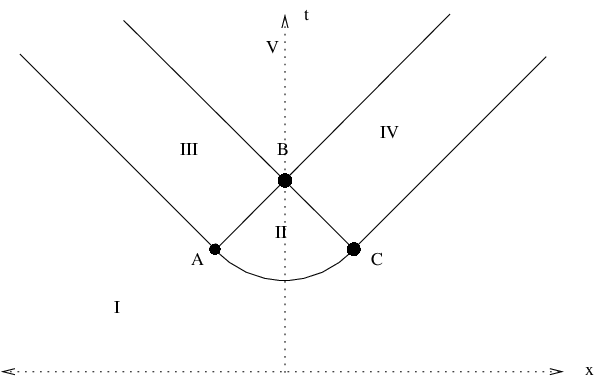
To illustrate the reflection in action, let us restrict attention to the triangular region

$$\Delta:=\{(t,x):t\geqslant 0;|t-x|,|t+x|\leqslant 10\}$$

and consider the initial data $\phi_{0},\phi_{1}$ associated to the linear solution

$$\phi^{({\operatorname{lin}})}(t,x)=1-\delta((t-2)^{2}+x^{2}-1)$$

where $\delta>0$ is a small constant (e.g. $\delta=10^{-3}$ is safe). Observe that $\phi^{({\operatorname{lin}})}$ lies between $-1$ and $1$ for most of $\Delta$, but exceeds $1$ in the disk $\{(t,x):(t-2)^{2}+x^{2}<1\}$. Thus we expect $\phi$ to follow $\phi^{({\operatorname{lin}})}$ until it encounters this disk, at which point it should reflect.

The actual solution $\phi$ can be described using Figure 1. In region I, $\phi$ is equal to the linear solution $\phi^{({\operatorname{lin}})}$. But $\phi^{({\operatorname{lin}})}$ exceeds $1$ once one passes the circular arc joining $A$ and $C$, and so a reflection must occur in region II; indeed, one has

$$\phi(t,x)=2-\phi^{({\operatorname{lin}})}(t,x)=1+\delta((t-2)^{2}+x^{2}-1)$$

in this region.

Once the solution passes $A$ and $C$, though, it turns out that the downward velocity of the reflected wave is now sufficient to drag $\phi$ off of the singular set⁸⁸ 8 An inspection of (1.14) suggests that the singular set must remain spacelike, thus the timelike portions of the set $\{\phi^{({\operatorname{lin}})}=1\}$ (which, in this case, are the left and right arcs of the circle $\{(t,x):(t-2)^{2}+x^{2}=1\}$) are not used as a reflective set for $\phi$. $\{\phi=+1\}$ (which, in this example, is the circular arc connecting $A$ and $C$). Indeed, in region III, we have

$$\phi(t,x)=1+\delta(2(t-2)x-1)$$

(note that this is the unique solution to the free wave equation that matches up with $\phi$ on regions I, II) and similarly on region IV we have

$$\phi(t,x)=1+\delta(-2(t-2)x-1).$$

Finally, on region V we have another solution to the free wave equation, which is now on a downward trajectory away from $\phi=+1$:

$$\phi(t,x)=1-\delta((t-2)^{2}+x^{2}+1).$$

If one were to continue the evolution of $\phi$ forward in time beyond $\Delta$ (extending the initial data $\phi_{0},\phi_{1}$ suitably), the solution would eventually hit the $\phi=-1$ barrier and reflect again, picking up further singularities propagating in null directions similar to those pictured here. Thus, while the solution remains piecewise smooth for all time, we expect the number of singularities to increase as time progresses, due to the increasing number of reflections taking place.

It is a routine matter to verify that the solution presented here verifies the properties (i)-(vi) on $\Delta$ (if $\delta$ is sufficiently small), and so is necessarily the limiting solution $\phi$, thanks to Theorem 1.3 (and the uniqueness theory in Section 3 below). We omit the details.

We shall shortly discuss the proof of Theorem 1.3, but let us first pause to discuss two techniques that initially look promising for solving this problem, but end up being problematic for a number of reasons.

Each of the nonlinear wave equations (1.1) enjoy a conserved stress-energy tensor $T^{(p)}_{\alpha\beta}$, and it is tempting to try to show that this stress-energy tensor converges to a limit $T^{(\infty)}_{\alpha\beta}$. However, the author found it difficult to relate this limit tensor to the limit solution $\phi^{(\infty)}$. The key technical difficulty was that while it was not difficult to ensure that derivatives $\phi^{(p)}_{u},\phi^{(p)}_{v}$ of $\phi^{(p)}$ converged in a weak sense to the derivatives $\phi^{(\infty)}_{u},\phi^{(\infty)}_{v}$ of a limit $\phi^{(\infty)}$, this did not imply that the magnitudes $|\phi^{(p)}_{u}|$, $|\phi^{(p)}_{v}|$ of the derivatives converged (weakly) to the expected limit of $|\phi^{(\infty)}_{u}|$, $|\phi^{(\infty)}_{v}|$, due to the possibility of increasing oscillations in the sign of $\phi^{(p)}_{u}$ or $\phi^{(p)}_{v}$ in the limit $p\to\infty$ which could cause some loss of mass in the limit. Because of this, much of the argument is instead focused on controlling this oscillation, and the stress-energy tensor conservation appears to be of limited use for such an objective. Instead, the argument relies much more heavily on pointwise conservation (or almost-conservation) laws such as (1.13), and on the method of characteristics.

Another possible approach would be to try to construct an approximate solution (or parametrix) to $\phi^{(p)}$, along the lines of (1.7), and show that $\phi^{(p)}$ is close enough to the approximate solution that the convergence can be read off directly (much as it can be from (1.7)). While it does seem possible to construct the approximate solution more or less explicitly, the author was unable to find a sufficiently strong stability theory to then close the argument by comparing the exact solution to the approximate solution. The difficulty is that the standard stability theory for (1.1) (e.g. by applying energy estimates to the difference equation) exhibits losses which grow exponentially in time with rate proportional to $p$, thus requiring the accuracy of the approximate solution to be exponentially small in $p$ before there is hope of connecting the approximate solution to the exact one. Because of this, the proof below avoids all use of perturbation theory⁹⁹ 9 Except, of course, for the fact that perturbation theory is used to establish global existence of the $\phi^{(p)}$., and instead estimates the nonlinear solutions $\phi^{(p)}$ directly. It may however be of interest to develop a stability theory for (1.1) which is more uniform in $p$ (perhaps using bounded variation type norms rather than energy space norms?). One starting point may be the perturbation theory for (1.8), explored recently in [1].

Our arguments are instead based on a compactness method. It is not difficult to use energy conservation to demonstrate equicontinuity and uniform boundedness in the $\phi^{(p)}$, so we know (from the Arzelá-Ascoli theorem) that the $\phi^{(p)}$ have at least one limit point. It thus suffices to show that all such limit points obey the properties (i)-(vi), and that the properties (i)-(vi) uniquely determine $\phi$. The uniqueness is established in Section 3, and is based on many applications of the method of characteristics. To establish that all limit points obey (i)-(vi), we first establish in Section 4 a number of a priori estimates on the solutions $\phi^{(p)}$, in particular obtaining some crucial boundedness and oscillation control on $\phi$ and its first derivatives, uniformly in $p$. In Section 5 we then take limits along some subsequence of $p$ going to infinity to recover the desired properties (i)-(vi).

We are indebted to Tristan Roy for posing this question, and Rowan Killip for many useful discussions, Ut V. Le for pointing out a misprint, to Patrick Dorey to pointing out the link to Liouville’s equation, and to the anonymous referee for many useful comments and corrections. The author is supported by a grant from the MacArthur Foundation, by NSF grant DMS-0649473, and by the NSF Waterman award.

Write $\langle u_{0},v_{0}\rangle:=(t_{0},x_{0})$. We already know that $\phi\langle u,v\rangle=\phi^{\prime}\langle u,v\rangle$ when $\langle u,v\rangle$ is sufficiently close to $\langle u_{0},v_{0}\rangle$ and $u+v\leqslant u_{0}+v_{0}$. We now make extend this equivalence to the right of $u_{0},v_{0}$:

Using space reflection symmetry (2.2), we can reflect the previous lemma and conclude

References

- [1] L. Kalyakin, Liouville equation under perturbation, Inverse Problems 17 (2001), 879–883.
- [2] J. Liouville, Sur l’equation aux differences partielles , J. Math. Pure Appl. 18(1853), 71–74.
- [3] B. Perthame, Kinetic formulation of conservation laws, Oxford Univ. Press, 2002.
- [4] C. D. Sogge, Lectures on Nonlinear Wave Equations, Monographs in Analysis II, International Press, 1995.
- [5] T. Tao, An explicitly solvable wave equation, preprint. Available at terrytao.wordpress.com/2009/01/23