Clock synchronization by remote detection of correlated photon pairs
Abstract
We present an algorithm to detect the time and frequency difference of independent clocks based on observation of time-correlated photon pairs. This enables remote coincidence identification in entanglement-based quantum key distribution schemes without dedicated coincidence hardware, pulsed sources with a timing structure or very stable reference clocks. We discuss the method for typical operating conditions, and show that the requirement in reference clock accuracy can be relaxed by about 5 orders of magnitude in comparison with previous schemes.
pacs
03.67.Hk, 07.05.Kf, 95.99.Sh, 42.65.Lm1 Introduction
Quantum key distribution (QKD) [1, 2, 3] is the only quantum information protocol that found its way into practical applications, and is currently in a stage of early commercial development. There are two families of protocols that use fundamentally different resources. The original QKD protocol BB84 [4] and its variants transmit single photons (or approximations thereof), while the other family [5] perform measurements on pairs of entangled photons. A few years ago, entanglement-based QKD protocols were viewed as equivalent to BB84 [6], and thus only of little interest for practical QKD due to their additional complexity. The new concept of device-independent QKD [7], and a returned awareness of classical side channels in prepare-and-send protocols revived interest in entanglement-based QKD schemes. Entangled photon pairs are efficiently prepared by spontaneous parametric down conversion (SPDC). Demonstrated for polarization-entangled pairs in 1995 [8], recent developments lead to the extremely bright sources available today [9, 10], so that entanglement-based QKD became a viable option.
The first step in establishing a key in such a scheme is the assignment of photodetection events to entangled photon pairs. Due to their strong temporal correlation (down to a few 100 fs) in typical pair sources [11], this assignment can be done via temporal coincidence identification. In typical laboratory experiments, as well as in early QKD implementations, a hardware channel was used to carry out this coincidence identification [12, 13]. Less hardware is required when coincidences are identified by comparing detection times given by good local clocks [14, 15] or a central GPS time reference [16].
In this paper, we present an algorithm that relaxes the rather stringent reference clock quality requirements for such a coincidence identification so that conventional crystal oscillators can be used. In section 2, we outline the general problem and present a robust coincidence tracking scheme. Section 3 covers the algorithm to find an initial time offset as implemented in earlier experiments [15, 17]. In sections 4-6 we extend this scheme in the presence of a frequency difference between the clocks necessary to permit the use of clocks with lower accuracy.
2 Photon pair identification with remote clocks

The identification of pairs is straightforward in any context in which a hardware coincidence gate can be used; this is the case in laboratory-based experiments or field setups with a dedicated synchronization channel.
The situation we address in this paper applies to cases where detection times of photons at the two distant locations [15, 16, 18] are recorded, and coincidences are identified based on these time stamps (see figure 1). This method requires stable and synchronous clocks used for the timestamping: A typical coincidence window is chosen to be slightly larger than the detector time jitter, which is on the order of 1 ns. The data acquisition for establishing a key out of measurements is supposed to run either continuously, or at least for a few 100 seconds. To maintain two clocks synchronized within after a time of 100 s, a relative accuracy of is required, a specification that is met by commercial Rubidium clocks. For longer operation times, this still may be insufficient unless either a timing signal is transmitted on a separate channel, or the time reference is provided by a central source.
Pair sources based on SPDC provide enough information in the streams of photodetection times and that such accurate clocks should not be necessary. As long as the pair events are initially identified, the drift of the clocks can be tracked directly from the coincidence signal. For this to work reliably, the rate of pair events must be significantly larger than the one for accidental coincidences due to background photons in the same time window , which is also a necessary condition for a obtaining a secure key in QKD. .
In its simplest form, a floating average of the time difference between true coincidence events can be used to track a drift of the reference time between the two sides. To illustrate this, and to evaluate the intrinsic clock stability necessary to follow the coincidence signature, we consider a realistic situation where the full width at half maximum of a coincidence time distribution due to detector jitter is ns. To estimate the center of this distribution with an uncertainty (one standard deviation) of ns, we need to average time differences over about
| (1) |
coincidence events. Even for very low coincidence detection rates of 100 counts per second (cps), it takes less than 0.2 seconds to get a sufficient number of events. Over that period, the clock should not drift such that an event leaves the coincidence window, which translates into a relative frequency accuracy requirement of over 100 ms. More realistic coincidence detection rates of 1-10 kcps require only a relative frequency accuracy of to over a period of 1 to 10 ms. Standard crystal oscillators easily exhibit a stability on that order, but may lack the accuracy. Thus, tracking the time difference in coincidences from a set of detection events permits to use these simpler reference oscillators during normal operation.
Two problems are left for recovering the coincidences from time stamps derived with respect to two separate clocks: First, the detection instances at both sides will have an unknown time offset between them. This is mainly due to the absence of a common origin of time with a high enough resolution, and propagation over the physical distance between the two sides. As long as two reference clocks have the same frequency, can be found by looking at the cross correlation between the two timing signals. We will elaborate this in the next section.
The second problem is related to the relative frequency difference between the two clocks due to a lack of accuracy. This is harder to solve, since the stream of time stamps and on each side has no intrinsic time structure: Both signal and background events follow a Poisson distribution11 1 While it has been shown that the light emerging from SPDC processes should exhibit super-poissonian statistics [19], this is typically not observed in practical SPDC systems with photon counting detectors because it is washed out by multi-mode effects on a time scale way below the detector resolution..
The two problems of finding time- and frequency differences from coincidence signals in the presence of uncorrelated background events are illustrated in figure 2. Trace (a) shows a distribution of detection events on side A, trace (b) reflects the event stream on side B, assuming that there is only a time offset , but no frequency difference between the two reference clocks. Trace (c) shows an event stream in side B both under presence of a time offset and a frequency difference. For convenience, we describe the relative frequency difference by a quantity , such that the detection times on both sides due to identified photon pairs are connected via
| (2) |
We now estimate how accurately and need to be determined. In a practical QKD implementation, the two timestamping clocks are coarsely synchronized with conventional means (e.g. using an NTP protocol [20]), so it can be assumed that will not exceed a few 100 ms. A coincidence time window may be about 1 to 5 ns wide, fixing the uncertainty in to be small enough to start coincidence time tracking as sketched above. Thus, needs to be known with a precision of a few , corresponding to an information of about 26 to 28 bit. For the tracking algorithm to take over, the relative frequency difference needs to be also known to an uncertainty of to . An upper bound for can be chosen to match a typical accuracy of standard crystal oscillators (e.g. ). Thus, of the two clocks needs to be found with a precision of to , equivalent to an information of 7 to 14 bits.
3 Finding the time offset
We first explain the algorithm to find the time offset , assuming the two reference clocks run at the same frequency (). Two streams of detection events and on both sides are translated into detection time functions
| (3) |
The cross correlation between these two functions,
| (4) |
has a peak at due to the correlated photodetection events on top of an unstructured but noisy base line from independent background detection events at both sides. The time offset is thus simply found by searching for the maximum in . In practice, is efficiently obtained from the timing sets via fast Fourier transformations (FFT) and their inverse,
| (5) |
with discrete arrays for , and of length (typically a power of 2). The high resolution necessary for (28 bits) renders a direct calculation impractical. It is possible, however, to obtain the coarse and fine part of separately with much smaller sample sizes. To illustrate how this works, we take the timing events , captured during an acquisition time , and map them onto the discrete arrays with a time resolution :
| (6) |
and accordingly. This is an efficient process which requires visiting each entry only once. The cross correlation array is obtained by the discrete version of equation (5), and its maximum located by a subsequent linear search in . If the cross correlation peak can be identified correctly, the result reflects up to a resolution , and modulo . Thus, applying this method with two different resolutions leads to a final with a resolution of 26 to 28 bit, while the individual FFTs are carried out at a moderate size of or less. The complete code for this procedure is available as open source [21].
It is beneficial to consider the influence of uncorrelated background events in this peak finding process. We assume a signal rate of true coincidences, and background rates and on both sides. The discrete arrays are built up from timestamps in a collection interval . The cross correlation peak will be made up by event pairs at the index , while the background event pairs are homogeneously distributed over all entries in following a Poisson distribution. The peak can be identified with sufficient confidence if its statistical significance , here defined as the ratio between the peak height above the base line and the standard deviation of the latter,
| (7) |
exceeds a certain numerical value. With the above rates, the peak value arising from signal pairs is
| (8) |
If we approximate the fluctuations on the base line of by a Gaussian distribution, the probability that a base line fluctuation gives rise to the largest value , and thus leads to a wrongly identified location of the cross correlation peak, is given by
| (9) |
A numerical evaluation of this quantity (see table 1) shows that for , leaves less than 1% probability of misidentifying the peak. Since can be directly estimated out of , it forms a good basis to gauge the success of the peak finding procedure in practice.
3.72 4.26 4.75 5.12 5.61 6.00 6.36 6.71 7.03
Care should be taken that events acquired over a time are uniformly distributed over the interval in the binning procedure of equation (6). Specifically, should be an integer number. Otherwise, uncorrelated background events are subject to an effective envelope and do not lead to a flat base line in the cross correlation array, so determination of and subsequent peak finding becomes difficult. This problem can also be addressed by removing the lowest Fourier components in equation (5) before the back transformation.
From equation (8) it can be seen that for given rates , , and , the only way to increase the success probability is to increase the number of time bins . For 100 kcps, =1 kcps, we need to exceed . Furthermore, the frequency difference of the reference clocks needs to be very small. A time stretch between the two clocks over an acquisition time exceeding the targeted resolution for reduces the statistical significance of the coincidence peak below a useful level. With parameters =2 ns and of a few seconds for the experiments carried out in [15, 17], reference clocks with a relative frequency difference were necessary, which were provided in the form of Rubidium oscillators.
Figure 3 shows the result of typical correlation arrays (rescaled in terms of ) from an experiment with event rates kcps, kcps and cps. Here, was chosen, and time resolutions ns for the coarse, and ns for the fine resolution. The peak exhibits for both resolutions, and the resulting time offset is ns.

4 Finding the time offset in the presence of a frequency difference
The only reason to use reference clocks with a relative frequency accuracy better than with the presented algorithms is to determine the initial time offset with a resolution on the order of 1 ns. Knowledge of the frequency difference to that accuracy and a reasonable stability is sufficient for tracking, so it is desirable to extract this information out of the timing events efficiently.
Finding both the time and frequency difference from the recorded timing signals in the presence of uncorrelated background events is equivalent of identifying a line in a plane of all possible pair events. This well-known pattern recognition problem is formally solved by the Hough transformation [22], which maps the pair time distribution onto the parameter space . As in the cross correlation method in the previous section, the pair searched for is the peak coordinate in the parameter space. However, we did not find an equally efficient high-resolution solution as for the one-dimensional problem in section 3.
A simpler method for determining is to estimate time offsets during relatively short acquisition intervals , shifted by a time with the method described in the previous section. The change in time offsets between these probe intervals is connected with the relative frequency difference via
| (10) |
However, it is necessary to reliably obtain the time offsets on the two sampling intervals – which itself is only possible with clocks with a sufficiently small . We now evaluate under which conditions this cross correlation step will succeed in finding a time offset .
For two clocks with , the contribution of correlated events will all end up in a single time bin in the discrete correlation array . For , the correlated events will spread out over roughly bin indices . This reduces not only the statistical significance for identifying a maximum, but also increases a timing uncertainty which in turn leads to an uncertainty in determining the frequency difference according to equation (10).
In order to identify the correlation peak with sufficient confidence according to equation (9), the statistical significance should exceed a threshold . For this, the timing resolution may have to be increased, forcing the true coincidences in less bins , up to to , or equivalently . This, together with equation (8) for the statistical significance, leads to an expression for the maximally acceptable frequency difference
| (11) |
for this strategy. In practice, the choice of a suitable size for the correlation array has not to be done before the time-consuming step of the cross correlation in equation (5). If with an initially chosen resolution the peak is not found, the array can be either re-partitioned in larger bins of width , or equivalently exposed to a moving average procedure until a statistically significant correlation peak is identified. Once the time offset is known with an accuracy , the relative frequency difference is known with an accuracy
| (12) |
In the low signal limit, where has to be chosen large enough to identify a peak at all, this results in a worst-case accuracy of .

We illustrate this method with experimental timing sets obtained from a non-optimized down conversion source with moderate background event rates ( kcps, kcps). Both timestamp units were referenced to crystal oscillators with a nominal frequency accuracy of 100 ppm.
With two segments of ns ms and a separation of s, convolution arrays were generated with a binning resolution of s. Since there were slowly varying changes in the background rates, the 20 lowest frequency entries (and their mirrors) were set to 0 before back transformation to , resulting in a smooth base line. The results are shown in the top traces of figure 4, without any significant correlation peaks. A subsequent re-binning with an effective width of ns reduced the noise level of the background sufficiently to allow the identification of the correlation peaks, resulting in time offsets of s, s, and subsequently in .
5 Iterative procedure to decrease timing and frequency uncertainty
The simple method for obtaining both and by analyzing correlations does typically not provide a sufficiently low uncertainty to start the tracking algorithm described in section 2. Therefore, additional steps are required. Knowledge of with uncertainty , the linear dependency of the timing uncertainty from according to equation (12), and the time offset with some accuracy suggest an iterative method for this purpose:
A set is prepared from , which is corrected with the initial values and (obtained as in section 4) via
| (13) |
With this set and the original set , new values for and are obtained. The reduction in uncertainty is given by the ratio according to equation (12), and is somewhat below an order of magnitude, or about 3 bit. This can be iterated, finally leading to values and with the targeted uncertainties (see appendix for the explicit algorithm).
6 A faster algorithm for finding the fine time offset
The iterative method in jointly finding and with sufficient accuracy converges only slowly because the time separation is typically not be very much larger than an acquisition time interval to keep the initial time for finding the coincidences low.
Once initial values for and are found, an alternative algorithm can be used: We begin with event pairs sets and , where the latter is corrected via equation (13) similarly as before. If the timing resolution for discretization is small enough (i.e., ), the arrays and are only sparsely populated. For with , signal events lead to coincidences in time bins with the same time bin indices . The sparse population of the arrays ensures then that the presence of a condition is very likely due to a true coincidence. For those pair events, the instantaneous time difference due to an inaccurately known and can be determined with an accuracy limited only by the time resolution of the detection system (typically dominated by detector timing jitter). Analysis of instantaneous time differences over the time interval finally reveals the parameters and with the intrinsic resolution of the system, after which the tracking algorithm can take over.

A distribution of time differences generated with this method from the time stamps used in section 4 is shown in figure 5(a). With one more iteration of the correlation algorithm, values s and were obtained to prepare the corrected set . The binning window for identifying coincidences was chosen as s. Out of the bins for both sets and , about 20 500 were occupied with one entry, and 75 and 191 with two events each; the rest were empty, thus forming sparse arrays.
One can visually identify a line structure, starting at about , and increasing to about towards the last of the 7839 coincidence candidates. Several of them are located away from this line, corresponding to bin pairs with accidental coincidences. The instantaneous time difference of true coincidences increases only slowly with the binning index , whereas the accidental coincidences can take arbitrary values. Thus, adjacent coincidence pairs with bin indices with a difference in their instantaneous time difference exceeding a modulus of are likely to contain at least one accidental coincidence. In a cleaning step, such pairs of adjacent candidates are simply removed. This step left only a small number of 384 coincidence candidates in the list, apparently without any accidentals (see figure 5(b)). A linear fit with a model with data from the remaining pairs returns offset correction parameters ns and . The error intervals from the fit appear overly optimistic, so we reconsider them, assuming a timing uncertainty of 1ns in instantaneous measurements. We finally arrive at ns and .
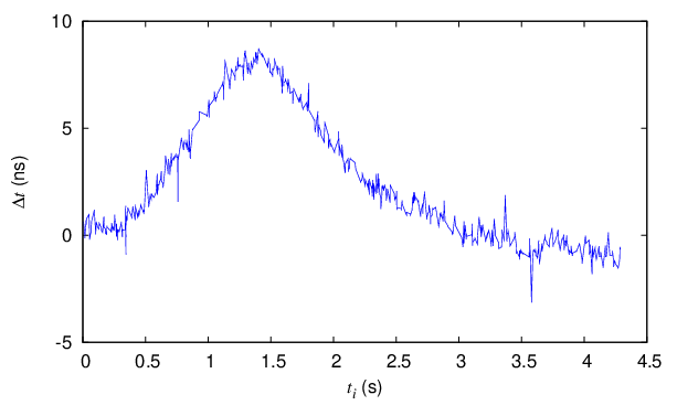
These values are sufficient to start the tracking algorithm sketched in section 2. Figure 6 shows the evolution of the instantaneous time difference , derived in a similar way as figure 5(b), but with the data corrected by the previously obtained constants for modeling the reference clock difference. One can recognize the slow drift of the reference oscillators, suggesting a stability around on a time scale of a second.
In conclusion, we presented an algorithm to remotely identify correlated photon pairs generated in a SPDC process from a stream of detection times without the need for a dedicated hardware channel, very stable and accurate pair of reference clocks or a central clock source, which may expose the classical infrastructure of a QKD system to a risk of compromise. This greatly reduces the technical complexity of entanglement-based QKD systems, making this part of an effort to simplify hardware by using intrinsic information in the photon pairs and bringing it closer to applications.
This work is supported by the National Research Foundation & Ministry of Education, Singapore, and partly by a joint program of quantum information research between DSO and NUS.
Appendix: Iterative algorithm for finding time- and frequency difference
An explicit algorithm for obtaining time- and frequency differences an from time sets with high precision comprises the following steps:
- 1.
Choose the limits for the maximum expected frequency and time differences and ; the observed rates and an expected rate can be used to check with equation (11) if this algorithm can be expected to be successful.
- 2.
Choose an acquisition time interval and a separation time interval , e.g. .
- 3.
Choose the smallest discretization time that is compatible with a high chance of successfully identifying the correct peak in the cross correlation. Pair this with a suitable value of for generating the arrays and according to equation (6).
- 4.
Generate the cross correlation array via FFT as in section 3.
- 5.
Find the index of the maximal value in and estimate its statistical significance according to equation (7).
- 6.
If is below a chosen significance limit , half the size of the array by adding entries pairwise, and go back to step 5; this doubles the effective time resolution . Otherwise, continue.
- 7.
Determine from the peak position and the effective time resolution of the last iteration of the previous step.
- 8.
With the time resolution in step 6, generate discrete arrays and for the second sampling interval, and determine from there .
- 9.
Determine from , and from equation (10).
- 10.
If in the last iteration is small enough to start the tracking as described in section 2, the algorithm is finished.
- 11.
Generate a modified set of event times according to
- 12.
Choose the same as in the last FFT, but reduce the time interval by less than the expected gain in accuracy given by ; typically, this reduction factor would be 4 or 8 corresponding to 2 or 3 bits in accuracy gain.
- 13.
Generate new and in the usual way from the original set and the modified set ; from the peak position in the new , determine the correction to . Usually, this adds 2 or 3 bits in accuracy to ; proceed similarly for the correction to .
- 14.
Continue with step 10.
References
References
- [1] Scarani, V, Bechmann-Pasquinucci, H, Cerf, NJ, Dusek, M et al. 2008, arXiv:0802.4155v2 [quant-ph] (to appear in Rev. Mod. Phys.)
- [2] Gisin, N and Thew, R 2007 Nature Photonics 1 165
- [3] Dûsek, M, Lütkenhaus, N and Hendrych, M 2006 Progress in Optics 49 381
- [4] Bennett, C and Brassard, G 1984 in Proceedings of the IEEE Int. Conf. On Computer Systems and Signal Processing (ICCSSP) 175 Bangalore, India
- [5] Ekert, A 1991 Phys. Rev. Lett. 67 661
- [6] Bennett, CH, Brassard, G and Mermin, ND 1992 Physical Review Letters 68 557
- [7] Acin, A, Brunner, N, Gisin, N, Massar, S et al. 2007 Phys. Rev. Lett. 98 230501
- [8] Kwiat, PG, Mattle, K, Weinfurter, H, Zeilinger, A et al. 1995 Phys. Rev. Lett. 75 4337
- [9] Fedrizzi, A, Herbst, T, Poppe, A, Jennewein, T and Zeilinger, A 2007 Optics Express 15 15377
- [10] Trojek, P and Weinfurter, H 2008 Appl. Phys. Lett.
- [11] Burnham, DC and Weinberg, DL 1970 Physical Review Letters 25 84
- [12] Poppe, A, Fedrizzi, A, Lorünser, T, Maurhardt, O et al. 2004 Optics Express 12 3865
- [13] Peng, CZ, Yang, T, Bao, XH, Jun-Zhang et al. 2005 Phys. Rev. Lett. 95 030502
- [14] Jennewein, T, Simon, C, Weihs, G, Weinfurter, H and Zeilinger, A 2000 Phys. Rev. Lett. 84 4729
- [15] Marcikic, I, Lamas-Linares, A and Kurtsiefer, C 2006 Applied Physics Letters 89 101122
- [16] Ursin, R, Tiefenbacher, F, Schmitt-Manderbach, T, Weier, H et al. 2007 Nature Physics 3 481
- [17] Ling, A, Peloso, MP, Marcikic, I, Scarani, V et al. 2008 Phys. Rev. A 78 020301
- [18] Erven, C, Couteau, C, Laflamme, R and Weihs, G 2008 Optics Express 16 16840
- [19] Holmes, CA, Milburn, GJ and Walls, DF 1989 Phys. Rev. A 39 2493
- [20] Mills, DL 1991 IEEE Trans. Communications COM-39 10 1482
- [21] The complete code for the QKD system is available under http://code.google.com/p/qcrypto
- [22] Hough, P 1959 in Kowarski, L, editor, Proceedings Int. Conf. High Energy Accelerators and Instrumentation 554–556 CERN appears as patent: P.V. Hough, A method and means for recognizing complex patterns, U.S. Patent 3,069,654, 1962