An estimate of the primordial non-Gaussianity parameter fNL using the needlet bispectrum from WMAP
Abstract
We use the full bispectrum of spherical needlets applied to the WMAP data of the cosmic microwave background as an estimator for the primordial non-Gaussianity parameter . We use needlet scales up to and the KQ75 galactic cut and find corrected for point source bias. We also introduce a set of consistency tests to validate our results against the possible influence of foreground residuals or systematic errors. In particular, fluctuations in the value of obtained from different frequency channels, different masks and different multipoles are tested against simulated maps. All variations in estimates are found statistically consistent with simulations.
Subject headings
cosmic microwave background — cosmology: observations — methods: statisticalI. Introduction
The theory of inflation predicts the fluctuations in the Cosmic Microwave Background (CMB) to be close to Gaussian distributed. However, a small degree of non-Gaussianity is generally present in all the inflationary scenarios. The primordial non-Gaussian signal predicted by many models can be parametrized in the form:
| (1) |
where is the primordial curvature perturbation field at the end of inflation and is the Gaussian part of the perturbation. The dimensionless parameter describes the amplitude of non-Gaussianity. The non-Gaussian part of the primordial curvature perturbation is a local functional of the Gaussian part and for this reason this kind of parametrization is often referred to as local non-Gaussianity. Local non-Gaussianity is predicted to arise from standard single-field slow-roll inflation [1, 39] as well as from alternative inflationary scenarios for the generation of primordial perturbations, like the curvaton [19, 38, 45] or inhomogeneous (pre)reheating models [18, 29, 30], or even from alternatives to inflation, such as ekpyrotic and cyclic models [34, 11]. Other models, such as DBI inflation [2] and ghost inflation [3], predict a different kind of primordial non-Gaussianity, called ”equilateral”, because the three point function for this kind of non-Gaussianity is peaked on equilateral configurations, in which the lengths of the three wavevectors forming a triangle in Fourier space are equal [13]. In this paper we will focus only on non-Gaussianity of the local type, described by equation 1. The interesting aspect of primordial non-Gaussianity is that the expected non-Gaussian amplitude varies significantly from model to model. Putting experimental bounds on is then equivalent to constraining primordial scenarios of inflation. For example standard single-field slow-roll inflation predicts at the end of inflation [1, 39] (and therefore a final value unity after general relativistic second-order perturbation effects are taken into account [9, 10]). Such a small value is not experimentally detectable and for this reason an eventual detection of a Gaussian signal in present and forthcoming CMB data will rule out single-field slow-roll inflation as a viable scenario. Motivated by these considerations many groups have attempted to measure using CMB datasets, and WMAP data in particular.
A detection of non-zero at more than the level was found by [55] using the WMAP data with the Kp0 galactic cut. The WMAP team found similar values but stating that only the value obtained with the slightly larger KQ75 galactic cut is reliable due to possible foreground residuals. In this case a value of was found. In both these cases, an extended version [13, 55, 54] of the [32] (KSW-method) based on the full bispectrum was used. Consistent results were found by [16] and [49] using parts of the bispectrum of spherical mexican hat wavelets [42] and the skewness of needlet coefficients. A recent estimate has now been made by [51] obtaining the smallest error bars on so far finding .
Recently, it was shown in [35] that needlet coefficients can be used to construct statistics which are directly related to the bispectrum. These statistics share most of the useful properties of the bispectrum, while at the same time they do present important advantages, especially in terms of robustness to masked data and computational rapidity. Motivated from these results, in this paper we will use the full bispectrum of needlet coefficients as an estimator of , introducing moreover a set of consistency tests to check the stability of our findings. In particular, we shall investigate whether changes in the estimated values of using different galactic cuts, different frequency bands and different multipoles are within the variations expected from simulations. Of course, variations in among these different cases which are significantly larger than statistical fluctuations might point out the presence of foreground residuals or other systematic effects that could have biased the estimate of .
II. Data
For this analysis we used the noise weighted average of the V and W frequency band of the WMAP 5 year CMB map, as well as the corresponding instrumental beam and noise properties. We have also performed the analysis on the individual Q (41 GHz), V (61 GHz) and W (94 GHz) bands. For masking out galactic foregrounds and point sources, we used the and mask supplied by the WMAP team. For particular cases, we also used the much smaller Kp12 mask (maintaining of the sky) as well as an extended KQ75+ mask. The KQ75+ mask is constructed from the KQ75 mask, extending the mask with 5 degrees along the rim, maintaining a total of of the sky. We have used the maps at Healpix11 1 http://healpix.jpl.nasa.gov resolution .
III. Method
III.1. Spherical needlets
Needlets are a new form of (second generation) spherical wavelets, which were introduced into functional analysis by ([46, 47]) and have attracted a lot of attention in the cosmological literature hereafter. The possibility to use needlets for the statistical analysis of spherical random fields, with a view to CMB applications, is first discussed in [5], where the stochastic properties of needlet coefficients are established and their possible roles for data analysis (spectrum estimation, Gaussianity testing) are described; further mathematical properties where then given in [6]. The first application to CMB data, in particular, for the analysis of cross-correlation of CMB and Large Scale Structure data was provided by [48]; a general presentation of the method for a CMB audience is given in [41], while in [27] the properties of different weighting schemes are investigated and compared. Further papers have applied needlets on CMB data, for issues such as map-making, spectrum estimation, detection of features and anisotropies ([21, 17, 20, 50]); more recently, needlets have also been considered for the analysis of directional data, with a view to high energy cosmic rays ([7]) and for the analysis of polarization data ([24, 25]), whereas extensions to the so-called Mexican needlets case are discussed by [23, 22], their stochastic properties being established in[36, 43].
The spherical needlet (function) is defined as
| (2) |
here, is a direction on the sphere, and is the frequency (multipole range) of the needlet and is a normalizing factor. The points can be identified with the pixel centres in the HealPix pixelization scheme. The number B defines the needlet basis such that only multipoles in the range are included, i.e. the function is zero outside this range. For details in the functional form of . please refer to [41] and references therein.
The advantages of needlets have already been discussed in several papers in the literature; in short, we recall that needlets do not rely on any tangent plane approximation; they are computationally very convenient, and inherently adapted to standard packages such as HealPix; they allow for a simple reconstruction formula (a property which is not shared by other wavelets systems); they are quasi-exponentially (i.e. faster than any polynomial) concentrated in pixel space. Moreover, needlets are exactly localized on a finite number of multipoles (the width of this support is explicitly known and can be specified as an input parameter, see Eq. 2)).
Random needlet coefficients can be shown to be asymptotically uncorrelated (and hence, in the Gaussian case, independent) at any fixed angular distance, when the frequency increases. This capital property is in general not shared by other wavelet systems (see ([36, 43])) and can be exploited in several statistical procedures, as it allows one to treat needlet coefficients as a sample of independent and identically distributed coefficients on small scales, at least under the Gaussianity assumption.
In this paper, for notational simplicity we shall take random needlet coefficients to be
Here denotes the frequency of the coefficient and denotes the direction on the sky. We are dropping a normalizing term this comes at no cost, because in this paper needlet coefficients always appear after normalization with their own standard deviation, so that this deterministic factor cancels. From the notational point of view, however, this allows a major simplification, as it permits to avoid considering different weights at different frequencies As before, the index can in practice be the pixel number on the HEALPix grid.
III.2. The needlets bispectrum
Starting from some highly influential papers ([28, 31]), the bispectrum has emerged in the last decade as the most promising statistics for the detection of non-Gaussianity in CMB data. To fix notation, we recall that, under the assumption of statistical isotropy for CMB radiation, we must have ([28])
where on the right hand side we have introduced the Wigner’s 3j coefficients, which are different from zero only for configurations of which satisfy the triangle conditions (see again [28, 31]). The unreduced bispectrum is identically zero in the Gaussian case; under non-Gaussianity, it can be estimated by
It was shown by ([31]) that, in the idealistic circumstance with the absence of masked regions, the bispectrum can constrain non-Gaussianity very efficiently, with a signal-to-noise ratio equal to unity for smaller than 10 at the Planck resolution. In the presence of masked regions, however, these properties deteriorate consistently; many statistical solutions have been discussed so far, see for instance [56, 55] for the most recent developments. A large literature has also focussed on the determinations of the multipole configurations where the signal-to-noise ratio should be expected to be stronger, in view of a given model: see for instance [4, 12, 8, 40, 55] and many others.
Our purpose in this paper is to combine ideas from the bispectrum and the needlets literature, to propose a needlet bispectrum method to test non-Gaussianity and estimate the nonlinearity parameter More precisely, we suggest to focus on the needlet bispectrum, defined by
where is the standard deviation of The needlet bispectrum was first considered in ([35]), and we refer to that paper for more discussion and details on its mathematical properties; the use of needlets for a non-Gaussianity test is also proposed in [49], where the focus is instead on the skewness of the coefficients (which can be viewed as a special case of the bispectrum, for . Of course, many other papers had previously used wavelet-related techniques to search for non-Gaussianity in CMB, see for instance [52, 14, 15, 44].
In short, to understand the motivations of our proposals, note that, denoting by the cardinality of the points (i.e., the number of points in the pixelization scheme, so that provides an approximation for the pixel area), and neglecting for simplicity beam factors, we have approximately
Write
hence we obtain
From the previous computations, it should be clear that the needlets bispectrum can be viewed as a smoothed and normalized form of the standard bispectrum estimator. As usual with wavelet techniques, the advantage is that, while the standard bispectrum is known to be heavily affected by the presence of masked regions, needlet coefficients are much more robust and consequently the needlet bispectrum makes up a more reliable statistics even for incomplete maps. Furthermore, the needlet bispectrum is computationally very convenient, as it does not require the evaluation of Wigner’s 3j coefficients, which is extremely time-consuming.
From the mathematical point of view, further properties of the needlets bispectrum are discussed by [35]; in particular, it is shown that, after normalization, is asymptotically Gaussian as the frequency increases. Furthermore, it can be shown that (under idealistic experimental circumstances) the values of the needlet bispectrum are asymptotically independent over different frequencies, so that chi-square statistics can be suitably implemented. In [35], some analytic discussion on the power properties of the needlet bispectrum for a pure Sachs-Wolfe model were also provided, showing that its expected valued diverges to infinity at high frequencies. Although those results were derived in a mathematical setting and did not take into account many features of CMB data, the simulations in the present paper show (in a much more realistic setting) that this procedure does have very satisfactory power properties in the presence of non-Gaussianity.
III.3. estimator
We will now use the needlets bispectrum for estimating by a minimization procedure. We define as
where the elements of the data vector are defined as for all combinations of satisfying the triangle condition. Here is the needlets bispectrum of the observed data and is the expectation value of the needlet bispectrum for a given value of . The correlation matrix is given by
The correlation matrix is obtained from Gaussian simulations. In order to avoid cumbersome numeric grid-calculations of , we seek an expression with a more explicit dependency of . In order to arrive at such an expression, we write out again the needlets bispectrum as
| (4) | |||||
As usual, the non-Gaussian ’s are assumed to be a combination of a linear (Gaussian) and a non-linear term: . This allows us to write the three-point correlations in ’s as
| (5) | |||||
The non-linear terms are assumed to be small, and thus we will neglect the higher order terms, . We will also neglect the pure Gaussian term, since the three point correlation function of a Gaussian field is zero. We insert the remaining terms into eq. 4 and find the mean value:
| (6) | |||||
where we have defined the quantity
which does not depend on to the first order in . Figure 1 shows a plot of a average needlet bispectrum from simulations with . Here the bispectrum is plotted along one of the indices , while the two other indices and are kept constant. In the same plot is also our first order approximation, . As we see, this approximation is fairly good for , and based on previous estimates ([33]), we will assume that does not have a value significantly higher than this.
We can now write the elements of the data vector of the as . In order to estimate , we need to find the value of that minimizes the
| (7) |
giving
| (8) |

III.4. The procedure to estimate
We will now show the full procedure we have used to estimate using the needlet bispectrum.
- 1.
Generate simulations of Gaussian sky maps using the best fit WMAP 5 year power spectrum. These are smoothed with an instrumental beam and noise is added. The maps are also multiplied with a mask for galactic cut, in order to remove foregrounds. A needlet transform is applied and the standard deviation of the needlet coefficients are found. This standard deviation is needed to find the needlet bispectrum as seen from eq. (4).
- 2.
Produce another Gaussian simulations. Mask, beam and noise properties are applied as above. The needlet coefficients are found and used to obtain the needlet bispectra, . These bispectra are used to find the covariance matrix . This converges very slowly, thus the need for such a large number of simulations.
- 3.
Generate non-Gaussian simulations ([37]) to find the mean first order non-Gaussian bispectrum, .
- 4.
Obtain the needlet bispectrum from the data and estimate using eq. 8
- 5.
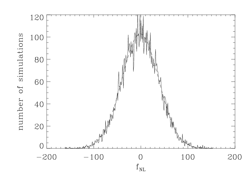
Generate a set of 10000 simulated Gaussian maps and estimate in the same manner from these maps in order to obtain the error bars on . This set of estimated values form a Gaussian distribution around . Figure 2 shows a histogram of the of the V+W frequency channel estimates plotted together with a Gaussian distribution. We see that the distribution of estimates is very close to Gaussian, so we will use the standard deviation as a measure of the uncertainty of the estimate.
IV. Results
IV.1. Estimates of
We used the above procedure to estimate from the WMAP data. The co-added V+W map as well as the single frequency bands Q, V and W were used. The estimated values of are listed in table 1 together with the error bars found from the simulations. For the analysis we used both the mask and the more aggressive mask for galactic cut in order to study potential effects from residual foregrounds.
We have used multipoles up to in the analysis. We tested different values of B in order to find the number of needlet scales from to which would yield an invertible covariance matrix. We found that the maximum number of scales which could be used was 31 scales, using . For comparison with the WMAP results we also used needlet scales including multipoles up to and . In table 1 as well as in the following text, we will use to specify the highest multipole included in the highest needlet scale. Note that this number may differ slightly from 1000, 700 and 500 depending on the exact value of specified. For , we used 30 scales with and for we used 31 scales with .
We see from the table that the best results obtained on the combined V+W band yields for the KQ75 cut and using the smaller KQ85 cut. We run simulations of unresolved point sources based on the procedure described in [33] and obtained a point source bias of for KQ75 and for KQ85 giving corrected values of and . We see that even for KQ75 a zero value for is excluded at about . In order to make sure that foregrounds are not influencing our results significantly, we also make an estimate on the much larger KQ75+ mask and obtain or taking into account unresolved point sources.
| freq. channel | mask | |||
|---|---|---|---|---|
| V+W | ||||
| V+W | ||||
| V+W | ||||
| V+W | ||||
| V+W | ||||
| V+W | ||||
| V+W (Raw) | ||||
| V+W (Raw) | ||||
| V+W (Raw) | ||||
| V | ||||
| V | ||||
| V | ||||
| V (Raw) | ||||
| V (Raw) | ||||
| W | ||||
| W | ||||
| W | ||||
| W (Raw) | ||||
| W (Raw) | ||||
| Q | ||||
| Q | ||||
| Q | ||||
| Q (Raw) | ||||
| Q (Raw) | ||||
| Combined V and W |
As we see there is a large improvement in error bars from to . This may seem at first sight surprising taking into account the fact that this range is noise dominated. However, this result is not unexpected if we take into account the way the needlets are constructed. Indeed, means that no needlet scale using information above is included. Nevertheless, from the previous description of the needlet systems it is easy to see that the information from multipoles close to the boundary value will receive very little weight in general. Of course, the next needlet scale will contain information below as well as above . Therefore, when extending the analysis to higher ’s we do not only exploit more multipoles, but we are also able to extract better information from the multipoles below .
Another test was performed to take advantage of the fact that the CMB should be independent of frequency, while the noise differs between the channels. A data vector was composed from the needlet bispectrum of both the individual V and W frequency channels.
| (9) |
The full covariance matrix in this case contains information about correlations between the frequencies, and should therefore enable us to get smaller error-bars on . However, for this analysis it was necessary to use only needlet scales from each frequency channel in order to get an invertible covariance matrix. And the result (shown in the bottom row of table 1) was not a large improvement from the analysis of the VW band at needlet scales. However this is our estimate for with the smallest error-bars while using the mask.
For the case for the V+W band with the KQ75 mask, we have also investigated the change in as a function of the number of needlet scales included. We thus included only the first 25 needlet scales (up to ), then the 26 first scales (up to and so on up to all 31 scales. The results are presented in table 2. As expected, we see that the error bars are decreasing with increasing . Differently from our case, in the optimal bispectrum estimation performed by the WMAP team and other groups error bars saturates earlier than lmax = 1000 because the full inverse covariance weighting scheme is not implemented and an approximation is used (whereas in this case the Monte Carlo approach used to estimate the bispectrum automatically accounts for this issue). Note however the WMAP error bars at lmax = 700 are still smaller than ours at lmax = 1000 because we don’t implement a minimum variance estimator and thus we don’t saturate the Rao-Cramer bound. Moreover an optimal bispectrum estimator with full inverse covariance weighting has been very recently implemented by Smith et al. 2008.
| V+W | V | W | Q | ||
|---|---|---|---|---|---|
| () | () | () | () | ||
| () | () | () | () | ||
| () | () | () | () | ||
| () | () | () | () | ||
| () | () | () | () | ||
| () | () | () | () | ||
| () | () | () | () |
IV.2. Consistency checks
We see from these results that the estimates using the mask differs notably from the estimates using the mask. This is particularly the case for the channel, when only considering scales up to . This estimate when using the mask () is much higher than the estimate found from the same map, using the mask (). We are therefore motivated to study simulations to find how often a change of mask triggers such a large difference in the estimate.
We consider two sets of CMB sky simulations, each set generated using the same random seed, and therefore identical. One set is multiplied with the mask, while the other is multiplied with the mask. Now we estimate for both sets, and find the difference between each estimate, and the corresponding estimate from the identical map with the other mask, . Then the mean value and standard deviation of is found.
For we found for the WMAP data, whereas the standard deviation for simulations. For , we found and . In the first case, the shift in when changing mask is as expected whereas in the latter case, the change is slightly high, but only at the level.
As a further test of consistency, we also considered the difference in estimate between and when using the galactic cut . However, a comparison with simulations reveal that have a standard deviation of . In other words, the difference in the two estimates is well within and is to be expected.
To test the variation of with increasing galactic cut, we estimated using the tiny Kp12 mask as well as the extended KQ75+ mask. We see that decrease when going from the smallest mask to KQ85 and KQ75, but increases slightly again to KQ75+.
At this point a test was implemented. Three identical sets of simulations were generated, and each set was multiplied with one of the KQ85, KQ75 and KQ75+ masks (we do not include the Kp12 mask as foregrounds are likely to be important for such a small mask). For each simulation, a data vector, , with two elements was formed from the difference in estimates between three different masks:
| (10) |
Of the simulations, were used to find a mean value and covariance matrix for . Then a value was found for each of the remaining simulations as follows:
| (11) |
A similar value was found from the values of the WMAP data maps. Then the values for the simulations were compared with that of the WMAP data.
The result was that of the simulations had a higher value of . We conclude that the variation of the estimate for different masks (larger than Kp12) are within expectations for a Gaussian map.
As a further check for possible foreground contamination we will check the variation of with frequency channel. We investigated this by estimating using simulated Gaussian CMB sky maps. For each simulated sky, three identical maps were generated. These maps were then smoothed with the instrumental beam of the Q, V and W frequency channel respectively, and noise was added independently to each of the maps. For each of these sets of simulations a needlet transform was performed using needlet scales in the range . Then the bispectra were found and was estimated, using between and of the needlet scales.
At this point we performed a test, similar to the one described above. First we tested the variation between the frequency channels when using all of the needlet scales. For every simulation, a data vector, , with two elements was formed from the difference in estimates between the channels.
| (12) |
The results using the KQ75 mask showed that only of the simulations had a higher value, than the WMAP data. This corresponds to a deviation.
To investigate whether this is consistent on several scales, we also performed the same test with some of the needlet scales removed. This was done using between and needlet scales. Finally we combined the data vectors from all these tests:
| (13) |
and used this to make a combined test. From the KQ75 results (shown in table 3) it seems that only by using all available scales we find a small inconsistency of the values between frequency channels. We repeated the latter test using the smaller KQ85 cut and found in this case that of the simulations had a higher concluding that foreground residuals do not appear to be causing the difference in for different channels.
| needlet scales | of sim. with higher | |
| all of the above | ||
To test the influence of foregrounds on the estimate of , we have estimated on the WMAP maps before foreground subtraction (raw maps). The results are listed in table 1. We see in particular for the Q band that the the value of is negatively biased by the presence of foregrounds. A similar result was also found in [55, 33]. Foreground residuals would thus be expected to give a too low value of . To check the power of our consistency test, we repeated the above test of the differences in estimated between frequency channels using 31 scales. We find that only of the simulations have a higher than for the WMAP data for the KQ75 cut, and none of the simulations have a similarly high for the KQ85 cut. The test thus shows a clear detection of foreground residuals in this case.
A similar test was now performed, but this time to study variation between different number of needlet scales (and thus also different ) used for the estimation:
| (14) |
where the superscript denotes number of needlet scales used to estimate the value. was found using equation (11) for the WMAP data as well as for the simulations according to the same procedure as above. This was done for the individual Q, V and W frequency channels, and for the combined V+W map. The test was also performed using a combined data vector from all the three frequency channels. The results (table 4) show that the variation in the estimate with respect to needlet scales is well within the expected bounds.
| Freq. channel | of sim. with higher |
|---|---|
| Q | |
| V | |
| W | |
| V + W | |
| combined Q, V and W |
V. Conclusions
We have tested an estimator for based on the needlet bispectrum [35]. We used the estimator to obtain best fit values of from the WMAP 5 year data, using the combined V+W map as well as the independent frequency channels. The error bars on obtained with the needlet bispectrum are significantly larger that those obtained by the optimal bispectrum estimator [51], but the needlet bispectrum still provides an important and independent test of consistency. We have further introduced a set of consistency tests based on the difference where 1 and 2 refer to different masks, different frequency channels or different number of multipoles. We compare the differences for the different cases to the values obtained in simulations.
We find our best estimate of using the combined bispectrum from the V and W channels giving using the KQ75 mask and , consistent within with the value of obtained by the WMAP team as well as with the values obtained by [55, 51] all using .
Using the combined map and , we obtained for KQ75 and using KQ85 (corrected for point source bias). This difference in using the two different masks was found to be within the limit from simulations and thus consistent with expectations. In order to further limit the risk of foreground contamination, we estimated on an extended KQ75 mask excluding of the sky giving .
Using the independent frequency channels and the KQ75 cut, we obtained for the Q band, for the V band and for the W band. Such a large difference in between the bands were found only in of the simulations. This is away from the expected value. This could be a sign of foreground residuals but could also well be a statistical fluke. We found the latter explanation to be more reasonable considering that for the smaller KQ85 mask of the simulations had a larger difference. Similar tests were made with values of obtained using different number of multipoles and channels, and no significant deviations from the expected differences were found. We therefore conclude that there are no convincing evidence of foreground residuals having influenced the estimated value of , even using the KQ85 galactic cut. However repeating these tests on the next release of the WMAP data and on Planck data will be necessary in order to confirm this claim.
References
- [1] Acquaviva, V., Bartolo, N., Matarrese, S. and Riotto, A. 2003, Nucl. Phys. B, 667, 119, arXiv:astro-ph/0209156
- [2] Alishahiha, M., Silverstein, E. and Tong, D. 2004, Phys. Rev. D , 70, 123505
- [3] Arkani-Hamed, N., Creminelli, P., Mukohyama, S. and Zaldarriaga, M. 2004, JCAP, 0404, 001
- [4] Babich, D., Creminelli, P., Zaldarriaga, M. 2004, Journal of Cosmology and Astroparticle Physics 8, 009
- [5] Baldi, P., Kerkyacharian, G., Marinucci, D. and Picard, D. 2006, Annals of Statistics, Vol. 37, No. 3, 1150-1171, arxiv:math.st/0606599
- [6] Baldi, P., Kerkyacharian, G. Marinucci, D. and Picard, D. 2007, Bernoulli, Vol. 15, n.2, pp. 438-463, arxiv: 0706.4169
- [7] Baldi, P., Kerkyacharian, G., Marinucci, D., Picard, D. 2008, Annals of Statistics, in press, arxiv: 0807.5059
- [8] Bartolo, N., Komatsu, E., Matarrese, S. and Riotto, A. 2004a, Phys. Rept., 402, 103
- [9] Bartolo, N., Matarrese, S. and Riotto, A. 2004b, JCAP, 0401, 003
- [10] Bartolo, N., Matarrese, S. and Riotto, A. 2004c, JHEP, 0404, 006
- [11] Buchbinder, E. I., Khoury, J. and Ovrut, B. A. 2008, Phys. Rev. Lett. , 100, 171302
- [12] Cabella, P., Hansen, F.K., Liguori, M., Marinucci, D., Matarrese, S., Moscardini, L., and Vittorio, N. 2006, MNRAS, 369, 819
- [13] Creminelli, P. et al. 2006 JCAP, 5, 4
- [14] Cruz, M., Cayon, L., Martinez-Gonzalez, E., Vielva, P. & Jin, J. 2007, ApJ, 655, 11
- [15] Cruz, M., Cayon, L., Martinez-Gonzalez, E., Vielva, P. 2006, MNRAS, 369, 57
- [16] Curto, A. et al 2008, in press, arXiv:0807.0231
- [17] Delabrouille, J., Cardoso, J.-F. , Le Jeune, M. , Betoule, M., Fay, G. & Guilloux, F. 2008, arxiv 0807.0773
- [18] Dvali, G., Gruzinov, A. and Zaldarriaga, M. 2004, Phys. Rev. D, 69, 023505
- [19] Enqvist, K. and Sloth, M. S. 2002, Nucl. Phys., B626, 395
- [20] Fay, G., Guilloux, F. , Betoule, M. , Cardoso, J.-F., Delabrouille, J. & Le Jeune, M. 2008a, Phys. Rev. D, D78, 083013
- [21] Fay, G. and Guilloux, F. 2008b, arxiv: 0807.2162
- [22] Geller, D. and Mayeli, A. 2007a, ArXiv.0706.3642
- [23] Geller, D. and Mayeli, A. 2007b, arxiv: 0709.2452
- [24] Geller, D. and Marinucci, D. 2008, arxiv: 0811.2935.
- [25] Geller, D., Hansen, F.K., Marinucci, D., Kerkyacharian and Picard, D. 2008, Physical Review D, D78, 123533
- [26] Górski, K.M., E. Hivon, A.J. Banday, B.D. Wandelt, F.K. Hansen, M. Reinecke, and M. Bartelmann, HEALPix: A Framework for High-resolution Discretization and Fast Analysis of Data Distributed on the Sphere, ApJ, 622, 759-771, 2005
- [27] Guilloux, F., Fay, G., Cardoso, J.-F.2007, arxiv 0706.2598
- [28] Hu, W. 2001, Physical Review D, 64, 8, id.083005
- [29] Kolb, E. W., Riotto, A. and Vallinotto, A. 2005, Phys. Rev. D, 71, 043513
- [30] Kolb, E. W., Riotto, A. and Vallinotto, A. 2006, Phys. Rev. D, 73, 023522
- [31] Komatsu, E. and Spergel, D.N. 2001, Physycal Review D, 63, 063002, arXiv:astro-ph/0005036
- [32] Komatsu, E., Spergel, D. N. & Wandelt, B. D. 2005, ApJ, 634, 14
- [33] Komatsu, E., et al. 2008, ApJS, in press, astro-ph/0803.0547v2
- [34] Koyama, K., Mizuno, S., Vernizzi, F. and Wands, D. 2007, JCAP, 0711, 024
- [35] Lan, X. & Marinucci, D. 2008a, Electronic Journal of Statistics, Vol. 2, pp.332-367, (2008), arXiv:0802.4020
- [36] Lan, X., Marinucci, D. 2008b, arxiv: 0805.4154
- [37] Liguori, M. et al. 2007, Phys. Rev. D, 76, 105016
- [38] D. Lyth and D. Wands 2002, Phys. Lett. B, 524, 5
- [39] Maldacena, J. M. 2003, JHEP, 0305, 013 (2003), arXiv:astro-ph/0210603
- [40] Marinucci, D. 2006, The Annals of Statistics 34, 1, arxiv;math/0502434
- [41] Marinucci, D., Pietrobon, D., Balbi, A., Baldi, P., Cabella, P., Kerkyacharian, G., Natoli, P., Picard, D., Vittorio, N., 2008, MNRAS, 383, 539
- [42] Martinez-Gonzalez, E. et al. 2002, MNRAS, 336, 22
- [43] Mayeli, A. 2008, arxiv: 0806.3009
- [44] McEwen J.D., Hobson M.P., Lasenby A.N., Mortlock, D.J. 2006, MNRAS, 371, L50
- [45] Moroi, T. and Takahashi, T. 2001, Phys. Lett. B, 522, 215, [Erratum-ibid. 539, 303 (2002)].
- [46] Narcowich, F.J., Petrushev, P. and Ward, J.D. 2006a, SIAM Journal of Mathematical Analysis 38, 2, 574
- [47] Narcowich, F.J., Petrushev, P. and Ward, J.D. 2006b, Journal of Functional Analysis 238, 2, 530
- [48] Pietrobon, D., Balbi, A., Marinucci, D. 2006, Physical Review D, 74, 043524
- [49] Pietrobon, D. et al. 2008a, arXiv:0812.2478
- [50] Pietrobon, D., Amblard, A., Balbi, A., Cabella, P., Cooray, A. & Marinucci, D. 2008b, Phys. Rev. D., D78, 103504
- [51] Smith, K. M., Senatore, L. & Zaldarriaga, M. 2009, arxiv: 0901.2572
- [52] Vielva P., Martinez-Gonzalez E., Barreiro B., Sanz J. & Cayon L. 2004, ApJ, 609, pp. 22
- [53] Yadav, A. S. et al 2007a, arXiv:0711.4933
- [54] Yadav, A. S., Komatsu, E. & Wandelt B. D. 2007b, ApJ, 664, 680
- [55] Yadav, A. S. & Wandelt, B. D. 2008, Phys. Rev. Lett, 100, 181301
- [56] Yadav, A.P.S., Komatsu, E., Wandelt, B.D. , Liguori, M., Hansen, F.K. and Matarrese, S. 2007, arXiv:0711.4933