Parallel dichotomy algorithm for solving tridiagonal SLAEs

A.V. Terekhov Email: andrew.terekhov@mail.ru Address: Institute of Computational Mathematics and Mathematical Geophysics, 630090,Novosibirsk,Russia Address: Budker Institute of Nuclear Physics, 630090, Novosibirsk, Russia

Abstract

A parallel algorithm for solving a series of matrix equations with a constant tridiagonal matrix and different right-hand sides is proposed and studied. The process of solving the problem is represented in two steps. The first preliminary step is fixing some rows of the inverse matrix of SLAEs. The second step consists in calculating solutions for all right-hand sides. For reducing the communication interactions, based on the formulated and proved main parallel sweep theorem, we propose an original algorithm for calculating share components of the solution vector. Theoretical estimates validating the efficiency of the approach for both the common- and distributed-memory supercomputers are obtained. Direct and iterative methods of solving a 2D Poisson equation, which include procedures of tridiagonal matrix inversion, are realized using the mpi technology. Results of computational experiments on a multicomputer demonstrate a high efficiency and scalability of the parallel sweep algorithm.

Keywords:

Parallel algorithm , Tridiagonal matrix algorithm (TDMA) , Thomas algorithm , Sweep Method , Poisson equation , Alternating Direction Method , Fourier Method

PACS

02.60.Dc , 02.60.Cb , 02.70.Bf , 02.70.Hm

1 Introduction.

The progress in numerical methods of solving "complex problems" is impossible without applying powerful parallel computer systems. Thus, it is necessary to investigate numerical algorithms that allow for efficient parallel implementation.

The problem of solving tridiagonal systems of linear algebraic equations [1, 2, 3] is one of the most frequently solved problems in computational mathematics. The tridiagonal SLAEs arise in three-point approximation of problems for ordinary differential equations of second order with constant and variable coefficients, and also in realization of difference schemes for equations in partial derivatives [4, 5, 6]. As a rule, tridiagonal SLAEs are solved using various versions of the direct difference equation method, that is, a sweep method: monotonic, nonmonotonic, flux and orthogonal [1, 2, 7, 8, 9].

Development and improvement of parallel sweep algorithms is of great interest, which is confirmed by numerous publications [3, 10, 11, 12, 13, 14, 15] concerned with this difficult problem. Analyzing papers dealing with this topic, we can conclude that presently available parallel sweep algorithms are insufficiently efficient and, what is more important, they are insufficiently scalable. The primary cause is that efficient, in a theoretical aspect, parallel algorithms realized on different multiprocessor computer systems become disadvantageous due to the presence of such operations as communications and synchronizations.

Solving problems by finite-difference methods frequently requires to solve not one, but a series of tridiagonal SLAEs with different right-hand sides, the number of problems in the series can reach thousands. Thus, the problem of designing an efficient parallel sweep algorithm for solving series of tridiagonal systems of equations deserves consideration.

In this paper, we propose a new approach to designing a parallel sweep algorithm for solving a series of tridiagonal SLAEs with a constant matrix and different right-hand sides. The process of solving the problem is subdivided into two steps. The first, preliminary step consists in fixing some rows of the SLAE inverse matrix by means of a sequential procedure. Then follows calculation of solutions for all right-hand sides; doing so, for increasing the algorithm efficiency using the formulated and proved main parallel sweep theorem, we proposed an original algorithm for calculating individual components from the solution vector.

2 Statement of the problem.

The series of systems of algebraic linear equations with a symmetrical constant tridiagonal matrix means

A{\bf X_{n}}={\bf F_{n}},\quad n=1,...,N.

(1)

A=\left\|\begin{array}[]{cccccc}b_{1}&a_{1}&&&&\Large 0\\ a_{1}&b_{2}&a_{2}&&&\\ &a_{2}&b_{3}&a_{3}&&\\ &&\ddots&\ddots&\ddots&\\ &&&a_{n-2}&b_{n-1}&a_{n-1}\\ 0&&&&a_{n-1}&b_{n}\\ \end{array}\right\|

, where $N$ is the number of problems in the series.

Assuming that system (1) is nondegenerate, we aim for designing a parallel algorithm for solving the problem and subsequent realizing on a multicomputer [16, 17].

Data decomposition.The computational and communication complexity of a parallel algorithm, hence, the execution time depend drastically on the way of decomposition of problem data. Let us dwell on the problem of mapping the data of problem (1) onto a set of processor elements (PEs).

Designing algorithms for distributed-memory supercomputers, it is necessary to take into account the fact that local data (data in the local memory of the same PE) are accessed much faster than data on a distant PE. Thus, even during designing the parallel sweep algorithm, we perform computing such as to minimize communication interactions by means of increasing the portion of local calculations (calculations performed with local data).

We ground the proposed parallel sweep algorithm on the following specification of data distribution between PEs:

Assuming that the number of PEs is $p$ , divide vectors ${\bf F_{n}}$ and ${\bf X_{n}}$ into subvectors ${\bf Q_{n_{i}},\,U_{n_{i}}}$ as follows¹¹ 1 The number of elements of a vector $\bf V$ , is denoted as size $\it{size}\{\bf V\}$ .:

{\bf F_{n}}=\left({\bf Q_{n_{1}}},{\bf Q_{n_{2}}},...,{\bf Q_{n_{p}}}\right)^{\mathrm{T}}=\left(f^{n}_{1},f^{n}_{2},...,f^{n}_{\it{size}\{\bf{F_{n}}\}-1},f^{n}_{\it{size}\{{\bf F_{n}}\}}\right)^{\mathrm{T}},

(2)

{\bf X_{n}}=\left({\bf U_{n_{1}}},{\bf U_{n_{2}}},...,{\bf U_{n_{p}}}\right)^{\mathrm{T}}=\left(x^{n}_{1},x^{n}_{2},...,x^{n}_{\it{size}\{\bf{X_{n}}\}-1},x^{n}_{\it{size}\{{\bf X_{n}}\}}\right)^{\mathrm{T}}.

(3)

The sizes of $\bf Q_{n_{i}}$ and $\bf U_{n_{i}}$ are chosen under the conditions

\begin{array}[]{l}size\{{\bf Q_{n_{i}}}\}=size\{{\bf U_{n_{i}}}\}\geq 2\quad i=1,...,p\\ \\ \sum_{i=1}^{p}\it{size}\{{\bf Q_{n_{i}}}\}=\sum_{i=1}^{p}\it{size}\{{\bf U_{n_{i}}}\}=\it{size}\{{\bf F_{n}}\}=\it{size}\{{\bf X_{n}}\}\end{array}

3.

Demand that the pair of subvectors $\left({\bf Q_{n_{i}}},{\bf U_{n_{i}}}\right)$ belong to PE number $i$ .
4.

The row of $A$ number $j$ is on the same PE as the pair of elements $\left(x^{n}_{j},f^{n}_{j}\right)$ from (2),(3).

We should note that the specification of decomposition of $\bf X_{n},\>F_{n}$ , and $A$ rules out absolutely duplication of the problem data. Exactly for this distribution we will design the parallel sweep algorithm for solving of problem (1).

3 Parallel sweep algorithm

3.1 Basic algorithm

Lemma 1.

Let the tridiagonal system of linear equations $A{\bf X_{n}}={\bf F_{n}}$ be divided into subsystems of the form

A_{i}{\bf U_{n_{i}}}={\bf Q_{n_{i}}},\quad i=1,...,p,

(4)

A_{i}=\left\|\begin{array}[]{cccccc}1&&&&&\Large 0\\ a_{l_{i}+1}&b_{l_{i}+2}&a_{l_{i}+2}&&&\\ &a_{l_{i}+2}&b_{l_{i}+3}&a_{l_{i}+3}&&\\ &&\ddots&\ddots&\ddots&\\ &&&a_{l_{i}+t_{i}-2}&b_{l_{i}+t_{i}-1}&a_{l_{i}+t_{i}-1}\\ 0&&&&&1\\ \end{array}\right\|,

t_{i}=size\{{\bf U_{n_{i}}}\},\quad l_{i}=\sum_{k=1}^{i-1}t_{i}

according to the proposed approach, and let we know the values of elements ²² 2 The first and last elements of some vector $\bf V$ , are denoted as $first\{{\bf V}\}$ and $last\{{\bf V}\}$ . $first\{{\bf U_{n_{i}}}\}$ $\quad last\{{\bf U_{n_{i}}}\}$ , then systems (4) can be solved independently, equality (3) will be fulfilled.

The proof of the lemma follows from the tridiagonal matrix of the structure itself.

Algorithm 1. Based on Lemma 1, we can propose the following parallel sweep algorithm

1.

Decompose initial system (1) into subsystems of form (4).
2.

Find solutions in boundary elements $first\{{\bf U_{n_{i}}}\},\,last\{{\bf U_{n_{i}}}\}$ .
3.

Compute $\bf X_{n}$ , by solving independently subsystems.

Thus, the parallel sweep algorithm enables to reduce the solution of problem (1) to $p$ independent subproblems of form (4), if values of $first\{{\bf U_{n_{i}}}\}$ and $last\{{\bf U_{n_{i}}}\}$ are known. However, we have still to solve the issue of the efficient way of computing "boundary" elements, i.e., it is necessary to design a parallel algorithm for computing an individual component of the solution vector $\bf X_{n}$ .

3.2 Computing arbitrary solution component.

Lemma 2.

Let $B$ be the symmetrical tridiagonal matrix. Then the value of the $k$ th component of solution vector $\left({\bf Y}\right)_{k}$ of the equation $B{\bf Y}={\bf F}$ can be found as

\left({\bf Y}\right)_{k}={\bf G_{k}}^{\mathrm{T}}{\bf F},

(5)

where the vector $\bf G_{k}$ is the solution of the following system of equations

B{\bf G_{k}}=\bf e_{k},

(6)

$\bf e_{k}$ is the unit vector.

Proof 1.

Let $\bf B_{.k}$ be designated by the $k$ th column of $B$ , and $\bf B_{k.}$ by the $k$ th row, respectively

B=\left({\bf B_{.1}},{\bf B_{.2}},...,{\bf B_{.n}}\right)=\left[\begin{array}[]{c}{\bf B_{1.}}\\ {\bf B_{2.}}\\ ...\\ {\bf B_{n.}}\end{array}\right]

By virtue of the definition of the inverse matrix $BB^{-1}=\bf I$ , the solution of system (6) is the $k$ th column of $B^{-1}$ and the $k$ th row (under the condition of matrix symmetry).

From this follows

\begin{array}[]{ll}{\bf G_{k}}=B^{-1}\bf{e_{k}}=\bf{B_{.k}^{-1}}=\left(\bf{B_{k.}^{-1}}\right)^{\mathrm{T}},\hskip 11.49994pt\left(Y\right)_{k}={\bf B}_{k.}^{-1}{\bf F}={\bf G^{\mathrm{T}}_{k}F}.\end{array}

(7)

Thus, the lemma has been proved.

Let us represent the algorithm for computing the arbitrary solution component for the series of tridiagonal equations of form (1).

Algorithm 2. For calculating $M$ different components of the solution vector $\left({\bf X_{n}}\right)_{k_{m}},$ $n=1,...,N$ ; $m=1,...,M$ from series of equations (1), ñëåäóåò:

1.

Find ${\bf G_{k_{m}}},\,m=1,...,M$ , as the solution of $A{\bf G_{k_{m}}}=\bf e_{k_{m}}$ .
2.

Define $\left({\bf X_{n}}\right)_{k_{m}}$ for the whole series as

$\left({\bf X_{n}}\right)_{k_{m}}={\bf G_{k_{m}}^{\mathrm{T}}}{\bf F_{n}},\>n=1,...,N,\quad m=1,...,M.$

Thus, Algorithm 2 makes it possible to find a separate component of the solution vector. It is important that for different $k_{m}$ the values of $\left({\bf X_{n}}\right)_{k_{m}}$ can be calculated independently. We should note that the vector ${\bf G_{k_{m}}}$ does not depend on the right-hand side of (1) , hence, it may be determined once for all $\bf F_{n}$ .

Let us consider Algorithm 2 in application to the parallel sweep algorithm. According to Algorithm 1, at the second step it is required to calculate values of elements $first\{{\bf U_{n_{i}}}\},\>$ $last\{{\bf U_{n_{i}}}\}$ for all PEs. The specified data decomposition assumes that only one subvector ${\bf U_{n_{i}}}$ and one subvector ${\bf Q_{n_{i}}}$ are placed on a single PE, therefore, each PE will compute two elements $\left(first\{{\bf U_{n_{i}}}\},last\{{\bf U_{n_{i}}}\}\right)$ from the solution vector. Parallel realization of Algorithm 2 entails a great difficulty, namely, according to (5), each PE will have to perform about $O(size\{{\bf X_{n}}\})$ operations regardless of the number of involved computational resources.

This causes the problem of modifying Algorithm 2 in such a manner that the number of operations per PE is about $\displaystyle O(size\{{\bf U_{n_{i}}}\})$ .

3.3 The main parallel sweep theorem.

We will start designing an efficient algorithm for computing "boundary" elements; for illustration, let us consider the following boundary-value problem

\begin{array}[]{lll}\displaystyle\frac{\mathrm{d}^{2}\varphi}{\mathrm{d}x^{2}}=-\rho(x);&\displaystyle\varphi(x_{0})=0,\quad\varphi(x_{1})=0\end{array}

(8)

As is known [18], the solution of problem (8) may be represented in the integral form via the corresponding Green function ³³ 3 In this case, we restrict ourselves only to the fact of its existence.

\varphi(x)=\int_{x_{0}}^{x_{1}}G(x,s)\rho(s)\mathrm{d}s.

(9)

Let us partition the interval $(x_{0},x_{1})$ by three points $\{x_{1/4},x_{1/2},x_{3/4}\}$ and define the right-hand side of (8) as

\rho(x)=\left\{\begin{array}[]{ll}0,&x_{0}\leq x\leq x_{1/4}\\ k(x),&x_{1/4}<x<x_{1/2}\\ 0,&x_{1/2}\leq x\leq x_{3/4}\\ 0,&x_{3/4}\leq x\leq x_{1}\\ \end{array}\right.

(10)

According to (9), the solution at the points of partitioning may be defined as

\begin{array}[]{ll}\displaystyle\varphi(x_{1/4})=\int_{x_{1/4}}^{x_{1/2}}G(x_{1/4},s)k(s)\mathrm{d}s,\quad\displaystyle\varphi(x_{1/2})=\int_{x_{1/4}}^{x_{1/2}}G(x_{1/2},s)k(s)\mathrm{d}s,\\ \displaystyle\varphi(x_{3/4})=\int_{x_{1/4}}^{x_{1/2}}G(x_{3/4},s)k(s)\mathrm{d}s.\end{array}

(11)

Another way for finding the solution of equation (8) at the point $x_{3/4}$ without calculating the integral of form (9), is as follows: since the point $x_{3/4}$ belongs to the interval $(x_{1/2},x_{1})$ he solution at it should satisfy the equation

\displaystyle\frac{\mathrm{d}^{2}\tilde{\varphi}}{\mathrm{d}x^{2}}=0,

(12)

with the boundary conditions

\begin{array}[]{ll}\displaystyle\tilde{\varphi}(x_{1/2})=\int_{x_{1/4}}^{x_{1/2}}G(x_{1/2},s)k(s)\mathrm{d}s,&\quad\tilde{\varphi}(x_{1})=0.\end{array}

(13)

It is extremely important (from the viewpoint of computation) that the solution of problem (12),(13) is represented analytically [19]

\tilde{\varphi}\left(x\right)=\varphi(x_{1/2}){\frac{x-{x_{1}}{}}{{x_{1}}-{x_{1/2}}}}.

(14)

Thus, the solution of (8) with the right-hand side (10) at the points $\{x_{1/4},x_{1/2},x_{3/4}\}$ is as follows

\begin{array}[]{ll}\displaystyle\varphi(x_{1/4})=\int_{x_{1/4}}^{x_{1/2}}G(x_{1/4},s)k(s)\mathrm{d}s,\quad\displaystyle\varphi(x_{1/2})=\int_{x_{1/4}}^{x_{1/2}}G(x_{1/2},s)k(s)\mathrm{d}s,\\ \displaystyle\varphi(x_{3/4})=\varphi(x_{1/2}){\frac{x_{3/4}-{x_{1}}}{x_{1}-x_{1/2}}}.\end{array}

(15)

Comparison of (11) with (15) in their computation complexity shows evident advantage of the latter because it is required to compute less integrals of form (9).

For the arbitrary function $\rho(x)$ we summarize the obtained result as a theorem.

Theorem 1.

It is required to find the solution of boundary problem (8) at points with the coordinates $\left\{x_{i}\mid x_{0}<x_{i}<x_{N},\;x_{i}<x_{i+1},\;i=1,...,\mathrm{N-1}\right\}$ . Then the following identity takes place

\varphi(x_{i})=\sum_{j=1}^{i}\alpha_{j}^{R}{\frac{x_{i}-x_{N}}{x_{j}-x_{N}}}+\sum_{j=i+1}^{N}\alpha_{j}^{L}{\frac{x_{i}-x_{0}}{x_{j}-x_{0}}},\quad i=1,...,N-1,

(16)

\begin{array}[]{cl}\displaystyle\alpha_{i}^{R}=\int_{x_{i-1}}^{x_{i}}G(x_{i},s)\rho(s)\mathrm{d}s,&i=1,...,N-1,\\ \\ \displaystyle\alpha_{i}^{L}=\int_{x_{i-1}}^{x_{i}}G(x_{i-1},s)\rho(s)\mathrm{d}s,&i=2,...,N.\end{array}

(17)

Let us formulate and prove the main parallel sweep theorem.

Theorem 2.

Let we have the nondegenerate system of linear algebraic equations with the tridiagonal matrix $A\mathbf{X}=\mathbf{F}$ of dimension $n$ . Then for each solution vector component from the set

\Omega=\left\{\left(\mathbf{X}\right)_{n_{i}}\left|1<n_{i}<n,\;n_{i}<n_{i+1},\;i=1,...,p\leq n\right.\right\}

(18)

the following identity holds true

\left(\mathbf{X}\right)_{n_{i}}=\sum_{j=1}^{i}\beta_{n_{j}}^{\mathrm{R}}\left(\mathbf{Z}_{n_{j}}^{\mathrm{R}}\right)_{n_{i}}+\sum_{j=i+1}^{p+1}\beta^{\mathrm{L}}_{n_{j}}\left(\mathbf{Z}_{n_{j}}^{\mathrm{L}}\right)_{n_{i}},

(19)

\begin{array}[]{ll}\displaystyle\beta_{n_{i}}^{\mathrm{L}}=\sum_{j=n_{i-1}}^{n_{i}-1}\mathbf{\textbf{(}F)}_{j}A^{-1}_{n_{i-1},j},&(n_{p+1}=n+1)\\ \displaystyle\beta_{n_{i}}^{\mathrm{R}}=\sum_{j=n_{i-1}}^{n_{i}-1}\mathbf{\textbf{(}F)}_{j}A^{-1}_{n_{i},j},&(n_{0}=1)\\ \\ \end{array}

(20)

\begin{array}[]{cc}B^{\mathrm{L}}_{k}\mathbf{Z}^{\mathrm{L}}_{k}=\mathbf{e^{\mathrm{L}}},\quad B^{\mathrm{R}}_{k}\mathbf{Z}^{\mathrm{R}}_{k}=\mathbf{e^{\mathrm{R}}},\end{array}

(21)

where

\begin{array}[]{cc}B^{\mathrm{L}}_{k}=\left\|\begin{array}[]{cccccc}b_{1}&c_{1}&&&&\Large 0\\ a_{1}&b_{2}&c_{2}&&&\\ &a_{2}&b_{3}&c_{3}&&\\ &&\ddots&\ddots&\ddots&\\ &&&a_{k-2}&b_{k-1}&c_{k-1}\\ 0&&&&0&1\\ \end{array}\right\|,&B^{\mathrm{R}}_{k}=\left\|\begin{array}[]{cccccc}1&0&&&&\Large 0\\ a_{k}&b_{k+1}&c_{k+1}&&&\\ &a_{k+1}&b_{k+2}&c_{k+2}&&\\ &&\ddots&\ddots&\ddots&\\ &&&a_{n-2}&b_{n-1}&c_{n-1}\\ 0&&&&a_{n-1}&b_{n}\\ \end{array}\right\|\end{array}

(22)

\mathbf{e}^{\mathrm{R}}=\left(1,0,0,...,0\right)^{\mathrm{T}},\;\mathbf{e}^{\mathrm{L}}=\left(0,...,0,0,1\right)^{\mathrm{T}}

Proof 2.

Let

\begin{array}[]{cc}\displaystyle\mathbf{X}=\sum_{j=1}^{p}\mathbf{X}^{j},&\quad\displaystyle\mathbf{F}=\sum_{j=1}^{p}\mathbf{F}^{j}\\ \end{array}

(23)

\displaystyle A\mathbf{X}^{j}=\mathbf{F}^{j}

Define elements of $\mathbf{F}_{j}$ as follows

\left(\mathbf{F}^{j}\right)_{i}=\left\{\begin{array}[]{ll}\displaystyle 0,&i<n_{j-1}\\ \\ \displaystyle\left(\mathbf{F}\right)_{i},&n_{j-1}\leq i<n_{j}\\ \\ \displaystyle 0,&i\geq n_{j}\end{array}\right.

(24)

Then the solutions $\left(\mathbf{X}_{j}\right)_{n_{j}-1},\;\left(\mathbf{X}_{j}\right)_{n_{j}}$ are unambiguously defined by the following expressions

\begin{array}[]{c}\displaystyle\left(\mathbf{X}_{j}\right)_{n_{j-1}}=A^{-1}_{n_{j-1}\mathbf{.}}\mathbf{F}_{j}=\sum_{k=n_{j-1}}^{n_{j}-1}A^{-1}_{n_{j-1},k}\left(\mathbf{F}_{j}\right)_{k}=\beta_{n_{i}}^{\mathrm{L}}\\ \\ \displaystyle\displaystyle\left(\mathbf{X}_{j}\right)_{n_{j}}=A^{-1}_{n_{j}\mathbf{.}}\mathbf{F}_{j}=\sum_{k=n_{j-1}}^{n_{j}-1}A^{-1}_{n_{j},k}\left(\mathbf{F}_{j}\right)_{k}=\beta_{n_{i}}^{\mathrm{R}}\end{array}

(25)

According to Lemma 1, define $\left(\mathbf{X}_{j}\right)_{n_{k}}$ for $1\leq k\leq j-2$ as

\begin{array}[]{l}B^{\mathrm{L}}_{n_{j}}\mathbf{X}^{\mathrm{L}}_{j}=\beta_{n_{j}}^{\mathrm{L}}\mathbf{e}^{\mathrm{L}},\\ \mathbf{X}_{j}^{\mathrm{L}}=\left(x^{\mathrm{L}}_{jn1},...,x^{\mathrm{L}}_{jn_{2}},...,x^{\mathrm{L}}_{jn_{j-2}},...,x^{\mathrm{L}}_{jn_{j-1}}\right)^{\mathrm{T}},\end{array}

(26)

and for $j+1\leq k\leq p$ as

\begin{array}[]{l}B^{\mathrm{R}}_{n_{j}}\mathbf{X}^{\mathrm{R}}_{j}=\beta_{n_{j}}^{\mathrm{R}}\mathbf{e}^{\mathrm{R}},\\ \mathbf{X}_{j}^{\mathrm{R}}=\left(x^{\mathrm{R}}_{jn_{j}},...,x^{\mathrm{R}}_{jn_{j+1}},...,x^{\mathrm{R}}_{jn_{p-1}},...,x^{\mathrm{R}}_{jn_{p}}\right)^{\mathrm{T}},\end{array}

(27)

Denoting

\begin{array}[]{cc}\mathbf{Z}_{n_{i}}^{\mathrm{R}}=\left(B^{\mathrm{R}}_{n_{i}}\right)^{-1}\mathbf{e}^{\mathrm{R}},&\mathbf{Z}_{n_{i-1}}^{\mathrm{L}}=\left(B^{\mathrm{L}}_{n_{i-1}}\right)^{-1}\mathbf{e}^{\mathrm{L}},\end{array}

(28)

we obtain the general formula for computing $\left(\mathbf{X}_{j}\right)_{n_{i}},\;i=1,...,p:$

\left(\mathbf{X}_{j}\right)_{n_{i}}=\left\{\begin{array}[]{l}\beta_{n_{j}}^{\mathrm{L}}\left(\mathbf{Z}_{n_{j}}^{\mathrm{L}}\right)_{n_{i}},\;i>j\\ \\ \beta_{n_{j}}^{\mathrm{R}}\left(\mathbf{Z}_{n_{j}}^{\mathrm{R}}\right)_{n_{i}},\;i\leq j\end{array}\right.

(29)

Substituting (29) into (23), yields (19).

The theorem has been proved.

Remark 1.

Since the vectors $\mathbf{Z}^{\mathrm{R,L}}_{n_{i}}$ do not depend on the right-hand side of (1), therefore, they may be defined once for the whole series of problems.

Remark 2.

If $A=A^{\mathrm{T}}$ , then according to Lemma 2 the quantities $\beta^{\mathrm{R,L}}_{n_{i}}$ may be defined as follows

\begin{array}[]{ll}\displaystyle\beta_{n_{i}}^{\mathrm{L}}=\sum_{j=n_{i-1}}^{n_{i}-1}\mathbf{\textbf{(}F)}_{j}\left(\mathbf{G}_{n_{i-1}}\right)_{j},\\ \displaystyle\beta_{n_{i}}^{\mathrm{R}}=\sum_{j=n_{i-1}}^{n_{i}-1}\mathbf{\textbf{(}F)}_{j}\left(\mathbf{G}_{n_{i}}\right)_{j},\end{array}

(30)

A{\bf G_{k_{m}}}=\bf e_{k_{m}}.

(31)

Based on Theorem 2, we formulate the algorithm for computing several components from the solution vector for the series of tridiagonal equations (1).

Algorithm 3.For computing $M$ different components of the solution vector $\left({\bf X_{n}}\right)_{k_{m}},$ $n=1,...,N$ ; $m=1,...,M$ from the series of equations (1), follow:

1.

Preliminary step. (Performed once for the whole series of problems).

1.1 Find ${\bf G_{k_{m}}},\,m=1,...,M$ , from the solution of equation (31).

1.2 Find ${\bf Z^{\mathrm{R,L}}_{k_{m}}},\,m=1,...,M$ from (21).
2.

Step of obtaining solutions. (Performed for each right-hand side F $\mathbf{F}_{n},\;n=1,...,N$ .)

2.1 Determine $\beta^{\mathrm{R,L}}_{k_{m}},\;m=1,...,M$ according to (30) .

2.2 Determine $\left({\bf X_{n}}\right)_{k_{m}},\;m=1,...,M$ according to (19).

Elementary counting of arithmetic operations at the preliminary step of Algorithm 3 shows that its realization by formulas (21) and (31) requires $\approx 24NP$ operations. For calculating components (18) by formulas (19),(30) requires $12N+M^{2}$ operations.

An important property of Algorithm 3 is that at each of four steps of the algorithm, calculations for different $k_{m}$ are independent. Therefore, the number of arithmetic operations per PE is $24NM/p$ for the first step and $(12N+M^{2})/p$ for the second, respectively.

Let us analyze the efficiency of Algorithm {1,3} without regard to communication interactions. As the criterion, we will enter the speedup

S=T_{1}/T_{p},

where $T_{1}$ is the number of operations for solving one problem from series (1) by a sequential sweep algorithm, and $T_{p}$ , by Algorithm {1,3}. Assuming $p=M$ , $T_{1}=8N$ , where $N$ is the number of unknowns and $T_{p}=\left(12N+2M^{2}\right)/p$ , we have ⁴⁴ 4 The obtained estimate (32) is conditional and represents rather the qualitative behavior of the speedup dependence on the number of unknowns and PEs.

S=\frac{8Np}{12N+p^{2}}

(32)

From (32) it follows that the speedup value increases monotonically as the number of PEs grows, and then starting from some $p>p_{0}$ decreases monotonically to zero.

Evidently, the minimal time of problem solution is achieved for the number of PEs

p_{0}=\max_{p}\left(\frac{8Np}{12N+p^{2}}\right)=\sqrt{6N},

ïðè ýòîì óñêîðåíèå ñîñòàâèò

S_{\max}=\frac{\sqrt{6N}}{3}.

Thus, the efficiency of parallel Algorithm {1,3} for the maximum possible speedup is $\approx 30\%$ . The remaining $70\%$ computations fall on "additional" operations for maintaining parallelism. From (30) and (19) it follows that the volume of these additional computations has order $O(p^{2})$ , where $p$ is the number of PEs.

For comparison, that difficulty is also characteristic of the algorithm proposed in [10, 20] , where for computing of $first\{{\bf U_{n_{i}}}\}$ and $last\{{\bf U_{n_{i}}}\}$ (in our designation) elements it is necessary to solve the tridiagonal system of equations with the number of unknowns equal to the number of PEs. Since the authors propose to calculate the solution by means of a sequential sweep algorithm version, the number of additional operations will be of order $O(p)$ , but contrary to (19), parallel computing is not allowed.

Thus, in Algorithm {1,3} as well as in the algorithm [10, 20], the time of computing $first\{{\bf U_{n_{i}}}\}$ and $last\{{\bf U_{n_{i}}}\}$ elements depends linearly on the number of PEs.

For increasing the efficiency of Algorithm {1,3}, we will task to reduce the number of arithmetic operations in realizing formula.

3.4 Parallel dichotomy algorithm for solving tridiagonal SLAEs.

It is required to calculate the components of the vector of solution defined in (18), it is assumed that $p=2^{p_{0}}-1\leq n,\;p_{0}>0$ .

Let us enter into the consideration the sets

\displaystyle\Omega_{i}=\left\{\left(\mathbf{X}\right)_{n_{j}}\left|\left(\mathbf{X}\right)_{n_{j}}\in\Omega,\;j=2^{\left\lfloor log_{2}p\right\rfloor+1-i}k,\;k=1,...,2^{i}-1\right.\right\}\backslash\left(\bigcup_{j=1}^{i-1}\Omega_{j}\right),

(33)

where $i=1,...,\left\lfloor\log_{2}(p)\right\rfloor+1$ .

It is evident that

\Omega=\bigcup_{i=1}^{\left\lfloor\log_{2}(p)\right\rfloor+1}\Omega_{i},\quad\quad\Omega_{i}\bigcap\Omega_{j}=\left\{\emptyset\right\},\;i\neq j

Theorem 3.

Let the components of the solution vector from the set $\Omega_{j},\;j\geq 1$ and the quanities $\beta^{\mathrm{R,L}}_{n_{i}},\;\mathbf{Z}^{\mathrm{R,L}}_{n_{i}},\mathbf{G}_{n_{j}},\;i=1,...,p,\;j=1,...,p-1$ be determined. Then for all $\left(\mathbf{X}\right)_{n_{i}}\in\Omega_{m},\;j<m\leq\left\lfloor\log_{2}(p)\right\rfloor+1$ , the following identity holds true

\left(\mathbf{X}\right)_{n_{i}}=\sum_{j=k_{1}+1}^{i}\beta_{n_{j}}^{\mathrm{R}}\left(\mathbf{Z}_{n_{j}}^{\mathrm{R}}\right)_{n_{i}}+\sum_{j=i+1}^{k_{2}-1}\beta^{\mathrm{L}}_{n_{j}}\left(\mathbf{Z}_{n_{j}}^{\mathrm{L}}\right)_{n_{i}}+\delta_{k_{1}}+\delta_{k_{2}},

(34)

\begin{array}[]{l}\delta_{k_{1}}=\left\{\begin{array}[]{ll}0,&k_{1}=0\\ \\ \left(\mathbf{X}\right)_{k_{1}}\left(\mathbf{Z}_{k_{1}}^{\mathrm{R}}\right)_{n_{i}}-\left(\mathbf{G_{k_{1}+1}}\right)_{k_{1}}\left(\mathbf{F}\right)_{k_{1}}\left(\mathbf{Z}_{k_{1}+1}^{\mathrm{R}}\right)_{n_{i}},&k_{1}>0\end{array}\right.\\ \\ \delta_{k_{2}}=\left\{\begin{array}[]{ll}0,&k_{2}=p+1\\ \\ \left(\mathbf{X}\right)_{k_{2}}\left(\mathbf{Z}_{k_{2}}^{\mathrm{L}}\right)_{n_{i}},&k_{2}<p+1\end{array}\right.\end{array}

where $k_{1}$ and $\;k_{2}$ are defined as follows

\displaystyle k_{1}=\min_{t,\;t<k,\;\left(\mathbf{X}\right)_{n_{t}}\in\left(\Omega_{j}\bigcup\{{X_{0}}\}\right)}(n_{i}-n_{t}),\quad\quad k_{2}=\min_{t,\;t>k,\;\left(\mathbf{X}\right)_{n_{t}}\in\left(\Omega_{j}\bigcup\{X_{p+1}\}\right)}(n_{t}-n_{i})

Proof 3.

Validity of the theorem follows from the fact that the known components from the set $\Omega_{j}$ partition the initial system according to Lemma 1 into independent subsystems and the solution of each subsystem can be represented as the sum of general solution of a homogeneous equation and a partial nonhomogeneous equation [21].

Based on Theorem 3, we formulate the efficient parallel algorithm for computing separate components from the solution vector

Algorithm 4. Dichotomy algorithm. Calculation of $M$ different components of the solution vector $\left({\bf X_{n}}\right)_{k_{m}},$ $n=1,...,N$ , $m=1,...,M$ from series of equations (1), requires:

1.

Preliminary step. (Performed once for the whole series of problems).

1.1 Find ${\bf G_{k_{m}}},\,m=1,...,M$ , from the solution of (31).

1.2 Find ${\bf Z^{\mathrm{R,L}}_{k_{m}}},\,m=1,...,M$ from (21).
2.

Step of obtaining solutions. (Performed for each right-hand side $\mathbf{F}_{n},\;n=1,...,N$ .)

2.1 Find $\beta^{\mathrm{R,L}}_{k_{m}},\;m=1,...,M$ according to (30) .

2.2 Calculate in ascending order of index $i=1,...,\left\lfloor\log_{2}(p)\right\rfloor+1$ the components of the solution vector $\left({\bf X_{n}}\right)_{k_{m}},\in\Omega_{i},$ using (34).

Remark 3.

Elements belonging to the same set $\Omega_{i}$ , can be calculated independently.

Let us analyze the issue of computational stability of Algorithm 4. We will say that Algorithm 4 is stable if for (34) for all $j$

{\left\|\mathbf{Z}^{\mathrm{R,L}}_{n_{j}}\right\|}_{C}\leq 1,

(35)

where

{\left\|\mathbf{X}\right\|}_{C}=\max_{i}\left\{\left|\left(\mathbf{X}\right)_{i}\right|\right\}

Let us formulate stability criterion of Algorithm 4.

Theorem 4.

Let the matrix $A$ have the diagonal dominance [2]

\left|b_{i}\right|\geq\left|a_{i}\right|+\left|c_{i}\right|,\quad i=2,...,N-1,

(36)

\left|b_{1}\right|\geq\left|c_{1}\right|,\quad\left|b_{N}\right|\geq\left|a_{N}\right|,

(37)

and at least in one of inequalities (36) or (37) , strict inequality holds, then Algorithm 4 is stable.

Proof 4.

If the matrix $A$ has the diagonal dominance, then obviously the matrices $B^{\mathrm{R,L}}_{k}$ also have a diagonal dominance. Following the sweep algorithm [7], the solution of system $B^{\mathrm{R}}_{k}\mathbf{Z}^{\mathrm{R}}_{k}=\mathbf{e^{\mathrm{R}}}$ may be written as

\begin{array}[]{ll}z^{\mathrm{R}}_{i}=\prod_{i=k}^{i+1}\alpha_{i},&i=1,...,k-1,\\ \\ \displaystyle\alpha_{i}=\frac{-c_{i}}{b_{i}+a_{i}\alpha_{i-1}},&i=2,...,k,\\ \\ \displaystyle\alpha_{1}=-c_{1}/a_{1}.\end{array}

From conditions (36),(37)follows the inequality $\left|\alpha_{i}\right|\leq 1$ [2], from where the following estimate takes place

\left|z^{\mathrm{R}}_{i}\right|=\left|\prod_{i=k}^{i+1}\alpha_{i}\right|\leq 1

We can similarly show that $\left|z^{\mathrm{L}}_{i}\right|\leq 1$ . Thus, the presence of diagonal dominance entails stability of Algorithm 4.

The theorem has been proved

Remark 5. Since for calculating all elements from the set $\Omega_{i}$ to perform $O(p)$ arithmetic operations regardless of the index $i$ , for realizing Algorithm 4, computing $p$ components from the solution vector requires $O(p\log_{2}p)$ operations.

Comparing the dependence of the speedup on the computing time (Fig. 2) for the dichotomy Algorithm {1,3} and algorithm [10, 20], we conclude that the dichotomy algorithm efficiency for few PEs is comparable with that of Algorithms {1,3} and [10, 20]. For a great number of PEs, Algorithms {1,3} and [10, 20] possess a nearly zero speedup, whereas the dichotomy algorithm efficiency remains quite high.

3.5 An example of applying the dichotomy algorithm.

For illustrating application of the dichotomy algorithm, we will consider the problem of definition

\Omega=\left\{\left(\mathbf{X}\right)_{1},\left(\mathbf{X}\right)_{2},\left(\mathbf{X}\right)_{3},,...,\left(\mathbf{X}\right)_{15}\right\}

Let us define the sets $\Omega_{i},i=1,...,\left\lfloor log_{2}15\right\rfloor+1=4$ according to (33).

\begin{array}[]{l}\Omega_{1}=\left\{\left(\mathbf{X}\right)_{8}\right\},\\ \Omega_{2}=\left\{\left(\mathbf{X}\right)_{4},\left(\mathbf{X}\right)_{12}\right\},\\ \Omega_{3}=\left\{\left(\mathbf{X}\right)_{2},\left(\mathbf{X}\right)_{6},\left(\mathbf{X}\right)_{10},\left(\mathbf{X}\right)_{14}\right\},\\ \Omega_{4}=\left\{\left(\mathbf{X}\right)_{1},\left(\mathbf{X}\right)_{3},\left(\mathbf{X}\right)_{5},\left(\mathbf{X}\right)_{7},\left(\mathbf{X}\right)_{9},\left(\mathbf{X}\right)_{11},\left(\mathbf{X}\right)_{13},\left(\mathbf{X}\right)_{15}\right\}.\end{array}

Then we calculate at first all elements from $\Omega_{1}$ , and then $\Omega_{2},\Omega_{3},\Omega_{4}$ (Fig. 3).

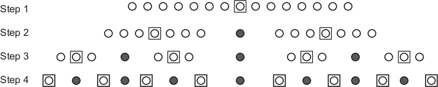
Thus, the initial system as a result of calculating at Step 1 the elements of $\Omega_{1}$ is divided into two independent subproblems, into four independent subproblems at Step 2 after calculating the elements from $\Omega_{2}$ , etc. until calculating the elements from $\Omega$ .

3.6 Nonsymmetrical matrices

Until now, it was supposed that the matrix of tridiagonal SLAE (1) symmetrical. This constraint restricts considerably the class of problems for which the parallel sweep algorithm is applicable.

Let us consider problem (1) with the symmetrical tridiagonal Jacobian matrix whose symmetrical elements have the same signs ( $a_{i}c_{i-1}\geq 0$ ). In this case, there exists a similarity transformation with the diagonal matrix $T$ such that the similar matrix $\hat{A}=T^{-1}AT$ is symmetrical [22]. The elements of the diagonal matrix $T$ are defined by the following recurrent relationships

\begin{array}[]{ccc}T=\rm{diag}\{t_{k}\},&t_{k+1}=t_{k}(a_{k+1}/c_{k})^{1/2},&k=1,...,N-1\end{array}

(38)

Thus, the series of SLAEs with the asymmetrical Jacobian matrix can be solved by the parallel sweep algorithm if the SLAE matrix is preliminary symmetrized via the similarity transformation.

In the general case, when the tridiagonal matrix is not symmetrical or cannot be symmetrized, equality (5) from Lamma 2 is no longer true. In this case, for determining rows of the inverse matrix, one can use the explicit representation of its elements [14, 27]

A_{ij}^{-1}=\left\{\begin{array}[]{rl}\displaystyle y_{i}z_{j}\prod_{k=1}^{j-1}\frac{a_{k}}{c_{k+1}},&i\leq j\\ \displaystyle z_{i}y_{j}\prod_{k=1}^{j-1}\frac{a_{k}}{c_{k+1}},&i\geq j\end{array}\right.

(39)

,where

\mathbf{Z}=\left(z_{1},z_{2},...,z_{n}\right)^{\mathrm{T}},

(40)

\begin{array}[]{cc}A\mathbf{Y}=\mathbf{e_{n}},&A\mathbf{Z}=\frac{1}{y_{1}}\mathbf{e_{1}}.\end{array}

(41)

4 Examples of applying the parallel sweep method.

For estimating the efficiency of the parallel algorithm of solving the series of tridiagonal SLAEs we propose, using it as a basis, a parallel realization of the methods of solving the Poisson equation. Let us consider the Dirichlet’s problem in a rectangle with the homogeneous boundary conditions $\bar{G}_{0}=\left\{0\leq x_{\alpha}\leq l_{\alpha},\,\alpha=1,2\right\}$

\begin{array}[]{c}\triangle u=-f(x),\quad x=\left(x_{1},x_{2}\right)\in G,\quad\left.u\right|_{\Gamma}=0.\end{array}

(42)

The corresponding difference approximation of second order of accuracy is

\begin{array}[]{c}\Lambda v=-f(x),\quad x\in\omega_{h},\quad\left.v\right|_{\gamma_{h}}=0\\ \displaystyle(\Lambda y)=\frac{1}{h_{1}^{2}}\left(y_{i+1,j}-2y_{i,j}+y_{i-1,j}\right)+\frac{1}{h^{2}_{2}}\left(y_{i,j+1}-2y_{i,j}+y_{i,j-1}\right),\end{array}

(43)

where

\bar{\omega}_{h}=\left\{x_{i}=\left(ih_{1},jh_{2}\right),\quad i=0,...,N_{1},\quad j=0,...,N_{2}\right\}

(44)

is a mesh with steps $h_{1}$ and $h_{2}$ , $\gamma_{h}$ is the mesh boundary.

We will consider the variable separation method (Fourier method) [2, 23] è Alternating Direction Method (ADI) [5, 2, 24] with application to solving problem (43).

a. Variable separation method. Since the function $u_{i,j}$ vanishes if îáðàùàåòñÿ â íóëü ïðè $j=0$ and $j=N_{2}$ , and the mesh function $f_{i,j}$ is given for $1\leq j\leq N_{2}-1$ , they may be represented as a series in eigenfunctions of the difference operator $\Lambda_{2}$ [25, 2]:

\left(\Lambda_{1}y\right)=\frac{y_{i+1,j}-2y_{i,j}+y_{i-1,j}}{h_{1}^{2}},\quad\left(\Lambda_{2}y\right)=\frac{y_{i,j+1}-2y_{i,j}+y_{i,j-1}}{h_{2}^{2}}

(45)

\begin{array}[]{cl}\displaystyle u_{i,j}=\sum_{l=1}^{N_{2}-1}\tilde{u}_{i}\left(l\right)\sin\left(\frac{\pi lj}{N_{2}}\right),&\quad 0\leq j\leq N_{2},\quad 0\leq i\leq N_{1},\\ \displaystyle f_{i,j}=\sum_{l=1}^{N_{2}-1}\tilde{f}_{i}\left(l\right)\sin\left(\frac{\pi lj}{N_{2}}\right),&\quad 1\leq j\leq N_{2}-1,\quad 1\leq i\leq N_{1}-1.\end{array}

(46)

Substituting (46) into (43) yields

\sum_{l=1}^{N_{2}-1}\left\{h_{1}^{-2}\left[\tilde{u}_{i+1}(l)-2\tilde{u}_{i}(l)+\tilde{u}_{i-1}(l)\right]-4h^{-2}_{2}\tilde{u}_{i}(l)\sin^{2}\frac{\pi l}{2N_{2}}+\tilde{f}_{i}(l)\right\}\sin\frac{\pi lj}{N_{2}}=0

(47)

From this, due to orthogonality of the eigenfunctions [2], the amplitudes of harmonics of the potential $\tilde{u}_{i}(l),\;l=1,...,N_{2}-1$ can be defined as the solution of the following system of equations

\begin{array}[]{lr}\displaystyle\tilde{u}_{i+1}(l)-\left(2+4\frac{h_{1}^{2}}{h_{2}^{2}}\sin^{2}\frac{\pi l}{2N_{2}}\right)\tilde{u}_{i}(l)+\tilde{u}_{i-1}(l)=-h_{1}^{2}\tilde{f}_{i}(l),&i=1,...,N_{1}-1,\\ \\ \tilde{u}_{0}(l)=\tilde{u}_{N_{1}}(l)=0.\end{array}

(48)

The sums (46) should be evidently computed using the fast discrete Fourier transform [2, 22], and for finding the solutions from the series of equations (48), we should use the sweep method.

Let us dwell on some aspects of realizing the parallel sweep algorithm within the scope of the variable separation method.

One of the constraints on the parallel sweep algorithm is that all SLAEs from the series of problems (1) contain the same fixed matrix. The tridiagonal matrices from (48) have the form

B_{l}=(T-d_{l}I),\quad d_{l}=4\frac{h_{1}^{2}}{h_{2}^{2}}\sin^{2}\frac{\pi l}{2N_{2}},\quad l=1,...,N_{2}-1,\quad

(49)

{\scriptstyle T=\left\|\begin{array}[]{cccc}\scriptstyle-2&\scriptstyle 1&&\scriptstyle\Large 0\\ \scriptstyle 1&\scriptstyle-2&\scriptstyle 1&\\ &\scriptstyle\ddots&\scriptstyle\ddots&\\ \scriptstyle 0&&\scriptstyle 1&\scriptstyle-2\\ \end{array}\right\|}

(50)

It is evident that for (49) the condition of matrix constancy for all right-hand sides is not fulfilled, hence, in this formulation, problem (48) cannot be solved efficiently by the proposed algorithm. However, we can extend Algorithm 1 for solving the series of Poisson equations on the fixed mesh

\triangle u=-f_{n}(x),\quad n=1,...,N.

(51)

In this case, it is required to solve the following problem

B_{l}u_{n}(l)=g_{n}(l),\quad l=1,...,N_{2}-1,\quad n=1,...,N.

(52)

The set of equations (52) may be considered as a set of problems of form (1) for the fixed $l$ .

b. Alternating Direction Method – belongs to the class of methods based on the concept of fixing. The solution of stationary problem (42) is found as the limit $t\rightarrow\infty$ of solution of the following unstationary problem

\frac{\partial u}{\partial t}=\Delta u-f

(53)

with the same boundary conditions.

Let us consider the Peaceman-Rachford scheme know also an ADI method [5, 24]. For this purpose, we represent the 2D difference Laplace operator as the sum of two operators $\Lambda=\Lambda_{1}+\Lambda_{2}$ (45). Then the iterative process of the ADI method for problem (53) has the form

\frac{u^{n+1/2}-u^{n}}{\tau^{(1)}_{n}}=\Lambda_{1}u^{n+1/2}+\Lambda_{2}u^{n}-f,

(54)

\frac{u^{n+1}-u^{n+1/2}}{\tau^{(2)}_{n}}=\Lambda_{1}u^{n+1/2}+\Lambda_{2}u^{n+1}-f.

(55)

The iterative parameters ${\tau^{(1)}_{k}},\;{\tau^{(2)}_{k}}$ should be chosen from the condition of minimum number of iterations. The problem of choosing the optimal parameters is comprehensively described, e.g., in [2, 4, 26, 6].

Let us consider a case when the region $\bar{G}$ is a square with the side $l=l_{1}=l_{2}$ and the mesh $\bar{\omega}$ is uniform with $N_{1}=N_{2}=N$ . Then in order that under any initial approximation $u_{0}$ the norm of initial error to be decreased $1/\varepsilon$ times

\parallel u_{n}-u\parallel_{D}\leq\varepsilon\parallel u_{0}-u\parallel_{D}

the number of iterations $n$ must satisfy the condition

n\geq n_{0}(\varepsilon)=0.2\ln\left(4N/\pi\right)\ln\left(4/\varepsilon\right).

(56)

Taking into account the fact that the sequence of optimal parameters $\tau^{(1)}_{k},\tau^{(2)}_{k},\quad k=1,...,n_{0}$ , is cyclic and the series of SLAEs (54),(55) for the fixed $n$ includes the constant matrix

C^{(1)}_{n}=\left(T-\frac{h_{1}^{2}}{\tau^{(1)}_{n}}I\right),\quad C^{(2)}_{n}=\left(T-\frac{h_{2}^{2}}{\tau^{(2)}_{n}}I\right)

we conclude that at the preliminary step, it is sufficient to solve merely $n_{0}$ tridiagonal SLAEs. It should be noted that the value $n_{0}$ is much less than the total number of equations whose solutions have to be found for achieving the desired accuracy.

5 Computational experiments.

As we have already mentioned, the parallel algorithms that are efficient from the theoretical viewpoint, when realized on supercomputers, may not ensure the expected reduction of the computation time. The primary reason is that in analyzing the efficiency of a particular algorithm, it is not easy to take into account all peculiarities of computer systems (memory operation, network throughput and latency, etc.). Thus, numerical experiments with model formulations of problems are an important stage of investigating parallel algorithms.

As the model problem we considered the Dirichlet problem for the Poisson equation

\begin{array}[]{c}\triangle u=-8\pi^{2}\sin(2\pi x)\sin(2\pi y),\quad x=\left(x_{1},x_{2}\right)\in G,\quad\left.u\right|_{\Gamma}=0.\end{array}

(57)

\bar{G}=\left\{0\leq x_{\alpha}\leq 1,\,\alpha=1,2\right\}

For solving problem (57) in the Fortran-90 language using the MPI technology we realized Fourier and ADI methods. The tridiagonal matrices were inverted by a parallel dichotomy algorithm. Equation (57) was approximated on uniform mesh (44) with $N_{1}=N_{2}=2^{k}$ nodes. For the ADI method, the value of prescribed accuracy $\varepsilon$ was $10^{-5}$ .

Figure 3a represents calculation domain decomposition for the Fourier method. Solution of the tridiagonal systems of equations was performed in the direction $k_{2}$ , and the Fourier transform was done in the direction $k_{1}$ . For the ADI method we chose a decomposition like a lattice (Fig. 3b) because the ADI method requires solution of tridiagonal SLAES in the directions $x$ and $y$ .

The computing time was estimated as the average time of solving one problem like (57) from a series of 100 problems

T_{avr}=\frac{\sum_{i=1}^{100}T^{i}}{100},

and the speedup time was calculated from the formula

S_{avr}=\frac{T_{avr}}{T_{1}},

$T^{i}$ is the time of solving problem (57) by the parallel algorithm, and $T_{1}$ – the sequential algorithm.

Test calculations were performed on an MBC-100k supercomputer of the Interdepartment Center of the Russian Academy of Sciences; the supercomputer is based on Intel Xeon four-core processors operating at 3 GHz in the Infiniband communication environment.

Results obtained for the dependence of the computing time ( $T_{avr}$ ) and speedup ( $S_{avr}$ ) for the Fourier and ADI methods are listed in Tables $1$ and $2$ , and in (Figs. 5a,5b,6a,6b).

Based on the obtained results, we will point out the following:

1.

For the Fourier and ADI methods, the dependence of the computing time on the number of processors is linear.
2.

For computing by the ADI method, starting from some number of processors, the speedup is superlinear because as the number of processors grows, the data volume per PE decreases, therefore, they can be located completely in a faster memory cache.
3.

The maximum performance of the Fourier method was $1700$ equations/ sec. for a $512\mathrm{x}512$ mesh $833$ eqs./sec for $1024\mathrm{x}1024$ , $417$ eqs./sec for $20482048$ , $161$ eqs./sec for $4096\mathrm{x}4096$ , $56$ eqs./sec for $8192\mathrm{x}8192$ , and $13$ eqs. for $16384\mathrm{x}16384$ , respectively.
4.

When the number of nodes in one direction exceeds several times the number of nodes in another direction, the efficiency of the parallel Fourier algorithm is between $80\%$ and $95\%$ (Figs. 6a and 6b).

size	512x512		1024x1024		2048x2048		4096x4096		8192x8192		16384x16384
NP	$\mathrm{T}_{avr}$	$\mathrm{S}_{avr}$	$\mathrm{T}_{avr}$	$\mathrm{S}_{avr}$	$\mathrm{T}_{avr}$	$\mathrm{S}_{avr}$	$\mathrm{T}_{avr}$	$\mathrm{S}_{avr}$	$\mathrm{T}_{avr}$	$\mathrm{S}_{avr}$	$\mathrm{T}_{avr}$	$\mathrm{S}_{avr}$
1	2.6e-02	-	1.1e-01	-	4.9e-01	-	2.11	-	11	-	-	-
4	6.2e-03	4.2	2.5e-02	4.5	1.2e-01	4	5.5e-01	3.8	2.8	3.9	-	-
8	2.6e-03	10	1.1e-02	10	6e-02	8.2	2.9e-01	7.2	1.6	6.7	-	-
16	1.4e-03	18.5	5.6e-03	21	3e-02	16.3	1.3e-01	16.2	0.8	13.8	-	-
32	8.5e-04	30	3e-03	38	1.3e-02	38	6.7e-02	31.4	0.4	27.5	1.78	-
64	7.9e-04	33	2e-03	58	6.6e-03	74	3.3e-02	63.9	0.19	58.3	0.95	54
128	5.9e-04	44	1.3e-03	84	4e-03	122	1.5e-02	140	9.6e-02	115.4	0.45	126
256	1.2e-03	22	1.2e-03	96	2.8e-03	175	9.4e-03	224	5e-02	221.6	0.24	237
512	-	-	2.2e-03	52	2.4e-03	204	6.8e-03	310	2.8e-02	395	1.4e-01	406
1024	-	-	-	-	-	-	6.2e-03	340	1.8e-02	611	7.7e-02	739

Table 1: Computing time (

\mathrm{T}_{avr}

) and speedup (

S_{avr}

) versus the number of processors for the Fourier method.

size	512x512			1024x1024			2048x2048			4096x4096
NP	$\mathrm{T}_{avr}$	$\mathrm{S}_{avr}$	$\mathrm{M}$	$\mathrm{T}_{avr}$	$\mathrm{S}_{avr}$	$\mathrm{M}$	$\mathrm{T}_{avr}$	$\mathrm{S}_{avr}$	$\mathrm{M}$	$\mathrm{T}_{avr}$	$\mathrm{S}_{avr}$	$\mathrm{M}$
1	0.9	-	-	8.7	-	-	48.17	-	-	202	-	-
4	8.5e-02	10.5	2x2	1.1	7.9	1x4	9.6	5	1x4	67	3	1x4
8	6.7e-02	13.4	8x1	0.84	10.3	1x8	7.3	6.6	1x8	34	5.9	1x8
16	2.6e-02	34	1x16	2.8e-01	31	1x16	2.3	21	1x16	12.2	16.8	1x16
32	2.0e-02	45	2x16	8.1e-02	107	2x16	0.94	51	2x16	7.7	28	1x32
64	2.5e-02	36	4x16	4.6e-02	189	4x16	0.29	166	4x16	2.8	71	1x64
128	-	-	-	3.7e-02	235	4x32	8.3e-02	580	4x32	1	180	4x32
256	-	-	-	3.4e-02	255	16x16	5e-02	963	16x16	0.3	721	16x16
512	-	-	-	3.3e-02	263	16x32	4.6e-02	1047	16x32	9.7e-02	2082	16x32
1024	-	-	-	4.2e-02	207	32x32	4.7e-02	1024	32x32	6.8e-02	2970	32x32

Table 2: Computing time (

\mathrm{T}_{avr})

and speedup (

S_{avr}

) versus the number of processors for the ADI method. (

M

, the number of processors in directions

k_{1}

and

k_{2}

, which enabled the minimal computing time.)

Thus, as a result of our computational experiments we registered the presently record efficiency in solving the Poisson equation on a multicomputer. These results were achieved due to applying the dichotomy algorithm for a series of tridiagonal SLAEs, which was specially designed for distributed-memory supercomputers. We should note that the proposed algorithms will be no less efficient, but even more for implementing on shared-memory multiprocessor computer systems because the communication interactions are minimal in that case.

6 Conclusions

The proposed parallel sweep algorithm for solving a series of tridiagonal systems of linear algebraic equations has validated its efficiency as a result of computational experiments. The main feature of the algorithm is that it is required at first to perform some preliminary computations whose complexity is comparable with solving one problem, and then solve a number of SLAEs for different right-hand sides with a nearly linear speedup. Thus, we have developed and investigated a promising method for solving a series of tridiagonal SLAEs, whose efficiency and scalability are record for today.

7 Acknowledgments.

The author is grateful to Prof. V. Malyshkin for fruitful discussions of the paper.

References

[1] S. K. Godunov and V. S. Ryabenkii, Diffrence Schemes (Nauka, Moscow, 1973) [in Russian].
[2] A. A. Samarskii and E. S. Nikolaev, Methods for Solving Mesh Equations (nNauka, Moscow, 1978) [in Russian].
[3] A. N. Konovalov, Introduction to Computational Linear Algebra Methods (Nauka, Novosibirsk, 1993), p. 159 [in Russian].
[4] A. A. Samarskii, Introduction to the Difference Scheme theory (Nauka, Moscow, 1971) [in Russian].
[5] N. N. Yanenko, The Fractional Pitch Method for Solving Problems of Mathematical Physics (Nauka, Novosibirsk, 1973) [in Russian].
[6] K.W. Morton, D.F. Mayers, Numerical solution of partial differential equations ,(Cambridge University Press, 2005 ) ,pp. 385, ISBN 0-521-60793-0.
[7] L. H. Thomas, Elliptic Problems in Linear Difference Equations over a Network. Technical Report (Columbia University Press, New York, 1949).
[8] S. K. Godunov, "On Numerical Solution of Systems of Ordinary Differential Equations of Forst Order," Uspekhi Mat. Nauk, No.3,pp. 171-174, 1961.
[9] V. P. Ilyin and Yu. I. Kuznetsov, Tridiagonal Matrices with Applications Nauka, Moscow, 1985) [in Russian].
[10] N. N. Yanenko, A. N. Konovalov, A. N. Bugrov, and G. V. Shustov, "On Organizing Parallel Computing and Sweep Parallelization,"Chislennye Metody Mekhaniki Sploshnoi Sredy, vol. 9, No. 7, pp. 139-146, 1978.
[11] X.-H. Sun, H. Zhang, and L. M. Ni, "Efficient Tridiagonal Solvers on Multicomputers," IEEE Trans. Comp., vol. 41, No. 3, pp. 286-296, 1992.
[12] M. M. Chawla, K. Passi, and R. A. Zalik, "A Recursive Partitioning Algorithm for Inverting Tridiagonal Matrices," Int. J. Computer Math., 35, pp. 153-158, 1990.
[13] . P. N. Swarztrauber, "A Parallel Algorithm for Solving general Tridiagonal Equations," Math. Of Comput., Vol. 33, No. 145, pp. 185-199, 1979.
[14] H. S. Stone, "An Efficient Parallel Algorithm for the Solution of a Tridiagonal Linear System of Equations," J-1 ACM, Vol. 20, No. 1. pp.27-38, 1973.
[15] A. Wakatani, "A Parallel and Scalable Algorithm for ADI Method with Pre-propagation and Message Vectorization," Parallel Computing 30 (2004), 1345-1359.
[16] V. V. Voevodin, VI. V. Voevodin, Parallel Computing (BHV-Peterburg, St. Petersburg, 2004), p. 608 [in Russian].
[17] V.Malyshkin, V.Korneev. Parallel Programming of Multicomputers. - (In series Textbooks of NSTU, 2006), p. 301 [in Russian].
[18] P. Morse and H. Feshbach , Methods of theoretical physics (repr. ed.), (McGraw Hill, Boston, 1999), ISBN 0-070-43316-X.
[19] V. F. Zaitsev and A. D. Polyanin, Reference Book of Ordinary Differential Equations (FIZMATLIT, Moscow, 2001), p. 576, ISBN 5-9221-0102-1.
[20] V. I. Paasonen, "Boundary Conditions of High-Order Accuracy at the Poles of Curvilinear Systems," Russian. Journ. of Num. Analysis and Math. Model., vol. 14, No. 4, pp. 369-382 (1999).
[21] A. O. Gelfond Calculation of Finite Differences (Fiz. Mat. Lit., Moscow, 1959) [in Russian].
[22] V. P. Ilyin, Methods of Finite Differences and Finite Volumes for Elliptic Equations (IVMiMG, Novosibirsk, 2001) [in Russian].
[23] R. W. Hockney, "A Fast Direct Solution of Poisson’s Equations Using Fourier Analysis," J. Assoc. Comput. Math., Vol. 12, pp. 95-113, 1965.
[24] D. W. Peaceman and H. H. Rachford, "The numerical solution of parabolic and elliptic differential equations", SIAM J. 3 (1955), 28-41.
[25] A. A. Samarskii and V. B. Andreev, Difference Methods for Elliptic Equations (Nauka, Moscow, 1976) [in Russian].
[26] E. L. Washspress, "Optimal Alternating-Direction-Implicate Iteration Parameters," SIAM J., vol. 10, No. 2. 1962.
[27] P. Schlegel, "The Explicit Inverse of a Tridiagonal Matrix," Math. Comput., Vol. 24, No. 111, p. 665.