Quantum chromodynamics at high energy
and statistical physics
Abstract
When hadrons scatter at high energies, strong color fields, whose dynamics is described by quantum chromodynamics (QCD), are generated at the interaction point. If one represents these fields in terms of partons (quarks and gluons), the average number densities of the latter saturate at ultrahigh energies. At that point, nonlinear effects become predominant in the dynamical equations. The hadronic states that one gets in this regime of QCD are generically called “color glass condensates”.
Our understanding of scattering in QCD has benefited from recent progress in statistical and mathematical physics. The evolution of hadronic scattering amplitudes at fixed impact parameter in the regime where nonlinear parton saturation effects become sizable was shown to be similar to the time evolution of a system of classical particles undergoing reaction-diffusion processes. The dynamics of such a system is essentially governed by equations in the universality class of the stochastic Fisher-Kolmogorov-Petrovsky-Piscounov equation, which is a stochastic nonlinear partial differential equation. Realizations of that kind of equations (that is, “events” in a particle physics language) have the form of noisy traveling waves. Universal properties of the latter can be taken over to scattering amplitudes in QCD.
This review provides an introduction to the basic methods of statistical physics useful in QCD, and summarizes the correspondence between these two fields and its theoretical and phenomenological implications.
Keywords:
Quantum chromodynamics , color dipole model , color glass condensate , stochastic fronts , traveling waves , reaction-diffusion 13.60.Hb , 12.38.-t1 Introduction to high energy scattering in QCD
The study of quantum chromodynamics in the high-energy regime has taken a new soar in the last 15 years with the wealth of experimental data that have been collected, first at the electron-proton collider DESY-HERA, and then at the heavy-ion collider RHIC. More energy in the collision enables the production of objects of higher mass in the final state, and thus the discovery of new particles. But higher energies make it also possible to observe more quantum fluctuations of the incoming objects, that is to say, to study more deeply the structure of the vacuum.
The well-established microscopic theory which describes the interactions of hadronic objects is quantum chromodynamics (QCD). (For a comprehensive textbook, see Ref. [1]). There are not many known analytical approaches to QCD, except perturbative expansions of observables in powers of the strong coupling constant which, thanks to asymptotic freedom, is justified for carefully chosen observables in special kinematical regimes. But fixed-order calculations in QCD are known to usually have a very limited range of applicability. This is because in the evaluation of Feynman graphs, the coupling constant always comes with “infrared” and “collinear” logarithms that are related to the phase space that is available to the reaction, that is to say, to kinematics. Resumming part of these logarithms is mandatory. All of them is too difficult. The question is to carefully select the dominant ones, and this is not at all easy.
At the HERA collider, electrons or positrons scattered off protons at the center-of-mass energy , exchanging a photon of virtuality . Through the scattering, one could probe partonic fluctuations of the proton (made of quarks and gluons) of transverse momenta , and longitudinal momentum fractions .
For a long time, the dominant paradigm had been that the collinear logarithms , that become large when is large compared to the QCD confinement scale , were the most important ones. As a matter of fact, searches for new particles or for exotic physics require to scrutinize matter at very small distances, and hence very large have to be considered. Perturbative series of powers of have to be fully resummed. The equation that performs this resummation is the celebrated Dokshitzer-Gribov-Lipatov-Altarelli-Parisi (DGLAP) equation [2, 3, 4].
However, once HERA had revealed its ability to get extremely good statistics in a regime in which is moderate (from to ) and very small (down to ) it became clear that infrared logarithms () could show up and even dominate the measured observables. The resummation of the series of infrared logs is performed by the Balitsky-Fadin-Kuraev-Lipatov (BFKL) equation [5, 6, 7]. The series (with appropriate coefficients) is the leading order (LO), while the series is the next-to-leading order (NLO), which has also been computed [8, 9]. The BFKL equation is a linear integro-differential equation.
At ultrahigh energy, the bare BFKL equation seems to violate the Froissart bound, that states that total hadronic cross sections cannot rise faster than . The latter is a consequence of the unitarity of the probability of scattering. The BFKL equation predicts a power rise with the energy of the form , where is positive and quite large ( to according to the effective value of that is chosen). The point at which the BFKL equation breaks down depends on the value of the typical transverse momentum which characterizes the observable (It is the photon virtuality in the case of deep-inelastic scattering). One may define the energy-dependent saturation scale in such a way that the BFKL equation holds for . For , the probability for scattering to take place is of order 1, and for , it would be larger than 1 if one trusted the BFKL equation. The saturation scale is a central observable, which we shall keep discussing in this review: It signs the point at which the linear (BFKL) formalism has to be corrected for nonlinear effects. The regime in which nonlinearities manifest themselves is a regime of strong color fields, sometimes called the color glass condensate (For the etymology of this term, see e.g. the lectures of Ref. [10]; for a review, see Ref. [11]).
The fact that unitarity is violated is not only due to the lack of a hadronic scale in the BFKL equation, which is a perturbative equation; Introducing confinement in the form of a cutoff would not help this particular problem. It simply means that still higher orders are needed. The NLO corrections to the BFKL kernel indeed correct this behavior in such a way that the description of the HERA data in the small- regime is possible by the BFKL equation. However, these corrections are not enough to tame the power-like growth of cross sections as predicted by the LO BFKL equation. It seems that a resummation of contributions of arbitrary order would be needed.
New equations were proposed well before the advent of colliders able to reach this regime. Gribov-Levin-Ryskin wrote down a model for the evolution of the hadronic scattering cross sections in the early 80’s [12, 13], and Mueller and Qiu derived a similar equation from QCD a bit later [14]. These equations are integral evolution equations with a nonlinear term, which basically takes into account parton saturation effects, that is to say, recombination or rescattering. The latter cannot be described in a linear framework such as the BFKL formalism. Subsequently, more involved QCD evolution equations were derived from different points of view. In the 90’s, McLerran and Venugopalan [15, 16, 17] proposed a first model, mainly designed to approach heavy-ion collisions. Subsequently, Balitsky [18], Jalilian-Marian, Iancu, McLerran, Weigert, Leonidov and Kovner (B-JIMWLK) [19, 20, 21, 22, 23] worked out QCD corrections to this model, and got equations that reduce to the BFKL equation in the appropriate limit. Technically, these equations actually have the form of an infinite hierarchy of coupled integro-differential equations (in Balitsky’s formulation [18]), of a functional renormalizaton group equation, or alternatively, of a Langevin equation (in Weigert’s formulation [23]). A much simpler equation was derived in 1996 by Balitsky [18] and rederived by Kovchegov in 1999 [24, 25] in a very elegant way within a different formalism. The obtained equation is called the Balitsky-Kovchegov equation (BK). The latter derivation was based on Mueller’s color dipole model [26], which proves particularly suited to represent QCD in the high energy limit.
The exciting feature of this kinematical regime of hadronic interaction from a theoretical point of view is that the color fields are strong, although, at sufficiently high energies, the QCD coupling is weak, authorizing a perturbative approach, and thus analytical calculations. In such strong field regime, nonlinear effects become crucial. But the conditions of applicability of the different equations that had been found had never been quite clear. Anyway, these equations are extremely difficult to solve, which had probably been the main obstacle to more rapid theoretical developments in the field until recently.
Furthermore, for a long time, the phenomenological need for such a sophisticated formalism was not obvious, since linear evolution equations such as the DGLAP equation were able to account for almost all data. But Golec-Biernat and Wüsthoff showed that unitarization effects may have already been seen at HERA [27, 28]. Their model predicted, in particular, that the virtual photon-proton cross section should only depend on one single variable , made of a combination of the transverse momentum scale (fixed by the virtuality of the photon ) and . This phenomenon was called “geometric scaling” [29]. It was found in the HERA data (see Fig. 1): This is maybe one of the most spectacular experimental result from HERA in the small- regime.

This observation has triggered many phenomenological and theoretical works. Soon after its discovery in the data, geometric scaling was shown to be a solution of the Balitsky-Kovchegov (BK) equation, essentially numerically, with some analytical arguments (see e.g. [31, 32, 33, 34]). The energy dependence of the saturation scale was eventually precisely computed by Mueller and Triantafyllopoulos [35]. Later, it was shown that the BK equation is actually in the universality class of the Fisher-Kolmogorov-Petrovsky-Piscounov (FKPP) equation [36, 37], and geometric scaling was found to be implied by the fact that the latter equation admits traveling wave solutions [38].
A first step beyond the BK equation, in the direction of a full solution to high energy QCD, was taken by Mueller and Shoshi in 2004 [39]. Actually, they did not solve the B-JIMWLK equations, but instead, they solved the linear BFKL equation with two absorptive boundary conditions, which they argued to be appropriate to represent the expected nonlinearities. Geometric scaling violations were found from their calculation, which should show up at any energies.
Subsequently, it was shown that high-energy QCD at fixed coupling is actually in the universality class of reaction-diffusion processes, studied in statistical physics, whose dynamics may be encoded in equations similar to the stochastic FKPP equation [40]. The Mueller-Shoshi solution was shown to be consistent with solutions to the latter equation. So high-energy QCD seems to be in correspondence with disordered systems studied in statistical physics. This correspondence has provided a new understanding of QCD in the high-energy regime, and it has proven very useful to find more features of high-energy scattering. The obtained results go beyond a solution to the B-JIMWLK equation, which in fact, thanks to the new picture, is seen to be incomplete.
Scope
The goal of this review article is to summarize the main ideas behind this conjectured correspondence between scattering at high-energy in QCD and some processes studied in statistical physics, as well as to introduce the QCD reader to the useful technical tools borrowed from statistical physics. We also feel that there is a cultural gap to be filled between statistical physics and particle physics. Indeed, statistical physicists are used to build simple toy models which contain the interesting physics, and whose main properties are likely to be independent of the details of the model, i.e. universal. In QCD, since the theory is well-established, we are often reluctant to give up some of its features to work out exact results in a toy model. One of our aims is to convince the reader that such a way of thinking is efficient in the case of high-energy QCD, by exhibiting results for QCD scattering amplitudes, obtained by looking for the universality class of the considered process, and that are believed to be exact.
Over the last few years, several hundreds of papers have appeared related to this subject, mainly issued from a very active though restricted community. Obviously, we cannot give a complete account of this abundant literature. As a matter of fact, some important recent developments had to be left out, for which we shall only provide references for the interested reader who might want to deepen his study in these directions. Concerning the correspondence itself, we do not attempt to establish a definite stochastic nonlinear evolution equation for QCD amplitudes, for to our judgement, this research line is not mature enough yet: A better understanding of the very saturation mechanism at work in QCD is definitely needed before one may come to this issue. Furthermore, it is not clear to us that a stochastic formulation would be a technical progress, since there are not many known methods to handle complicated stochastic equations. We feel that the same is true for the search for effective actions that would include so-called Pomeron loops. We also do not address the developments based on the boost-invariance symmetry that scattering amplitudes should have: This would drive us too far off the main focus of this review. As for more phenomenological aspects, we only discuss the basic features of total cross sections without attempting to address other observables such as diffraction. We do also not address the issue of next-to-leading effects such as the running of the QCD coupling. This discussion, though crucial if one wants to make predictions for actual colliders, would probably only be technical in its nature: There is no conceptual difference between the fixed coupling and the running coupling case. Here, only basic phenomenological facts brought about by this new understanding of high-energy QCD are addressed, namely geometric scaling and diffusive scaling.
Outline
The outline goes as follows. The next section is devoted to describing scattering in QCD from a -channel point of view, relying essentially on the parton model or rather on an interpretation useful in the high-energy limit, the color dipole model. Once this picture is introduced, it is not difficult to understand the correspondence with reaction-diffusion processes occuring in one spatial dimension, whose dynamics is captured by equations in the university class of the Fisher-Kolmogorov-Petrovsky-Piscounov (FKPP) equation. We then explain how traveling waves appear in this context. In Sec. 3, we study in greater detail a toy model for which many technics (field theory, statistical methods) may be worked out completely. This model however ignores spatial dimensions, and thus, does not account for traveling waves. We summarize the state-of-the-art research on equations in the universality class of the FKPP equation in Sec. 4. Finally, we come back to QCD, discussing the relevance of one-dimensional-like models in the FKPP class, and showing how noisy traveling waves may show up in the actual data.
2 Hadronic interactions in a -channel picture and analogy with reaction-diffusion processes
In this section, we shall introduce the physical picture of high-energy scattering in the parton model. In particular, the color dipole model [26] is described since it is particularly suited to address high-energy scattering, especially close to the regime in which nonlinear effects are expected to play a significant role. In a second part, we shall argue that high-energy scattering is a peculiar reaction-diffusion process.
2.1 Parton model and dipoles
2.1.1 General picture
For definiteness, let us consider the scattering of a hadronic probe off a given target, in the restframe of the probe and at a fixed impact parameter, that is to say, at a fixed distance between the probe and the center of the target in the two-dimensional plane transverse to the collision axis. In the parton model, the target interacts through one of its quantum fluctuations, made of a high occupancy Fock state if the energy of the reaction is sufficiently high (see Fig. 2a). As will be understood below, the probe effectively “counts” the partons in the current Fock state of the target whose transverse momenta (or sizes ) are of the order of the one that characterizes the probe: Roughly speaking, the amplitude for the scattering off this particular partonic configuration is proportional to the number of such partons.
The observable that is maybe the most sensitive to quantum fluctuations of a hadron is the cross section for the interaction of a virtual photon with a hadronic target such as a proton or a nucleus. The virtual photon is emitted by an electron (or a positron). What is interesting with this process, called “deep-inelastic scattering”, is that the kinematics of the photon is fully controlled by the measurement of the scattered electron. The photon can be considered a hadronic object since it interacts through its fluctuations into a quark-antiquark state. The latter form color dipoles since although both the quark and the antiquark carry color charge, the overall object is color neutral due to the color neutrality of the photon. The probability distribution of these fluctuations may be computed in quantum electrodynamics (QED). Subsequently, the dipole interacts with the target by exchanging gluons. The dipole-target cross section factorizes at high energy. One typical event is depicted in Fig. 2a.
Dipole models [41, 42] have become more and more popular among phenomenologists since knowing the dipole cross section enables one to compute different kinds of observables. Like parton densities, the latter is a universal quantity, that may be extracted from one process and used to predict other observables. Different phenomenological models may be tried for the dipole cross section. QCD evolution equations may even be derived, as we shall discover below. An accurate recent study of the foundations of dipole models may be found in Ref. [43, 44].
In QCD, the state of a hadronic object, encoded in a set of wave functions, is built up from successive splittings of partons starting from the valence structure. This is visible in the example of Fig. 2a: The quark and the antiquark that build up, in this example, the target in its asymptotic state each emit a gluon, which themselves emit, later on in the evolution, other gluons. As one increases the rapidity by boosting the target, the opening of the phase space for parton splittings makes the probability for high occupation numbers larger. Indeed, the probability to find a gluon that carries a fraction (up to ) of the momentum of its parent parton (which may be a quark or a gluon) is of order for small . There is a logarithmic singularity in , meaning that emissions of very soft gluons (small ) are favored if they are allowed by the kinematics. The splitting probability is of order 1 when the total rapidity of the scattering is increased by roughly , where the convenient notation has been introduced. Only splittings of a quark or of a gluon into a gluon exhibit the singularity. Therefore, at large rapidities, gluons eventually dominate the partonic content of the hadrons.
The parton model in its basic form, where the fundamental objects of the theory (quarks and gluons) are directly considered, is not so easy to handle in the high-energy regime. One may considerably simplify the problem by going to the limit of large number of colors (), in which a gluon may be seen as a zero-size quark-antiquark pair. Then, color-neutral objects become collections of color dipoles, whose endpoints consist in “half gluons” (see Fig. 2b). There is only one type of objects in the theory, dipoles, which simplifies very much the picture. Furthermore, going to transverse coordinate space (instead of momentum space, usually used in the DGLAP formalism) by trading the transverse momenta of the gluons for the sizes of the dipoles (through an appropriate Fourier transform) brings another considerable simplification. Indeed, the splittings that contribute to amplitudes in the high-energy limit are the soft ones, for which the emitted gluons take only a small fraction of the momentum of their parent (the latter being very large). Therefore, the positions of the gluons (and thus of the edges of the dipoles) in the plane transverse to the collision axis are not modified by subsequent evolution once the gluons have been created. Thus, the evolution of each dipole proceeds through completely independent splittings to new dipoles.
 |
 |
| (a) | (b) |
We will now see how this picture translates into a QCD evolution equation for scattering amplitudes, first in the regime in which there are no nonlinear effects. In a second step, we will try and understand how to incorporate the latter.
2.1.2 BFKL equation from the dipole model

(a)

(b)

(c)
The building up of the states of each hadron is specified by providing the splitting rate of a dipole whose endpoints have transverse coordinates into two dipoles and as the result of a gluon emission at position . It is computed in perturbative QCD and reads [26]
| (1) |
Dipole splittings are independent. After some rapidity evolution starting from a primordial dipole, one gets a chain of dipoles such as the one depicted in Fig. 3.
The elementary scattering amplitude for one projectile dipole off a target dipole is independent of the rapidity and reads [26]
| (2) |
If the target is an evolved state at rapidity , then it consists instead in a distribution of dipoles. The (forward elastic) scattering amplitude is just given by the convolution of and , namely
| (3) |
Let us examine the properties of . To this aim, it is useful to decompose the coordinates of the dipoles in their size vector (resp. ) and impact parameter (resp. ). In the limit in which the relative impact parameters of the dipoles is very large compared to their sizes, we get the simplified expression
| (4) |
and thus the scattering amplitude decays fast as a function of the relative impact parameter. If instead the relative impact parameter is small (of the order of the size of the smallest dipole), we get
| (5) |
where , , and the integration over the angles has been performed.
Equation (4) means that the dipole interaction is local in impact parameter: It vanishes as soon as the relative distance of the dipoles is a few steps in units of their size. Eq. (5) shows that only dipoles whose sizes are of the same order of magnitude interact. These properties are natural in quantum mechanics. Thus the amplitude in Eq. (3) effectively “counts” the dipoles of size of the order of at the impact parameter (up to ), with a weight factor .
An evolution equation for the amplitude with the rapidity of the scattering can be established. It is enough to know how the dipole density in the target evolves when rapidity is increased, since all the rapidity dependence is contained in in the factorization (3), and such an equation may easily be worked out with the help of the splitting rate distribution (1). It reads [26]
| (6) |
where . The very same equation holds for . The elementary scattering amplitude only appears in the initial condition at , which is not shown in Eq. (6). In a nutshell, the integral kernel encodes the branching diffusion of the dipoles. The total number of dipoles at a given impact parameter grows exponentially, and their sizes diffuse. The appropriate variable in which diffusion takes place is . (This is due to the collinear singularities in Eq. (1).) This equation is nothing but the BFKL equation. A complete solution to this equation, including the impact-parameter dependence, is known [45].
An important property of the amplitude is that it is boost-invariant. This property is preserved in the BFKL formulation. We could have put the evolution in the projectile instead of the target, or shared it between the projectile and the target: The result for the scattering amplitude would have been the same. In a frame in which the target carries units of rapidity and the projectile , the amplitude reads
| (7) |
is the density of dipoles found in a dipole of initial size after evolution over steps in rapidity. If , one recovers Eq. (3). If , then all the evolution is in the projectile instead.
The amplitude is related to an interaction probability, and thus, it must be bounded: In appropriate normalizations, has to range between 0 and 1. But as stated above, the BFKL equation predicts an exponential rise of with the rapidity for any dipole size, which at large rapidities eventually violates unitarity. Hence the BFKL equation does not provide a complete account of high-energy scattering in QCD.
2.1.3 Unitarity and the Balitsky-Kovchegov equation
It is clear that one important ingredient that has been left out in the derivation of the BFKL equation is the possibility of multiple scatterings between the probe and the target. Several among the dipoles in Eq. (7) may actually interact with the dipoles in the other hadron simultaneously. The only reason why such interactions may not take place is that (see Eq. (2)), and thus the probability for two simultaneous scatterings is of order , which is suppressed. But this argument holds only as long as the dipole number densities are of order . If (which is also the point above which the unitarity of is no longer preserved in the BFKL approach), then it is clear that multiple scatterings should occur.
In order to try and implement these multiple scatterings, we introduce the probability that there be no scattering between a dipole and a given realization of the target with total rapidity , that we shall denote by . Let us start with a system in which the evolution is fully contained in the target. We increase the total rapidity by boosting the projectile (initially at rest) by a small amount . Then there are two cases to distinguish, depending on whether the dipole splits in the rapidity interval . In case it splits into two dipoles and , the probability that the projectile does not interact is just the product of the probabilities that each of these new dipoles do not interact. This is because once created, dipoles are supposed to be independent. In summary:
| (8) |
Taking the average over the realizations of the target and the limit , we get
| (9) |
(See Fig. 4 for a graphical representation.)

We see that this equation is not closed: An evolution equation for the correlator is required. However, we may assume that these correlators factorize
| (10) |
This assumption is justified if the dipoles scatter off independent targets, for example, off the nucleons of a very large nucleus. Writing , we get the following closed equation for :
| (11) |
which is the Balitsky-Kovchegov (BK) equation [24, 25]. Note that if one neglects the nonlinear term, one gets back the BFKL equation (6) (written for instead of ). A graphical representation of this equation is given in Fig. 5.

It is not difficult to see analytically that the BK equation preserves the unitarity of : When becomes of the order of 1, then the nonlinear term gets comparable to the linear terms in magnitude, and slows down the evolution of with , which otherwise would be exponential.
Let us go back to Eqs. (8),(9) and instead of assuming the factorization of the correlators (10), work out an equation for the two-point correlator . From the same calculation as before, we get
| (12) |
where we have introduced the notation . (See Fig. 6a for the corresponding graphical representation.)

(a)

(b)
This equation calls for a new equation for the 3-point correlators, and so on. The obtained hierarchy is nothing but the Balitsky hierarchy [18] (see also Ref. [46, 47]) restricted to dipoles. We refer the reader to [48, 49] (see also Ref. [50]) for the detailed relationship of this equation to the B-JIMWLK formalism. Note in particular that the factorized correlators (10) is a solution of the whole hierarchy, and is actually a good approximation to the solution of the full B-JIMWLK equations. This statement was first made after the results of the numerical solution to the JIMWLK equation worked out in Ref. [51].
We may wonder why there are no terms involving one-point functions in the right handside of the previous equation. Actually, such terms would correspond to graphs like the one of Fig. 6b, in which, for example, two dipoles merge. They are expected to occur if saturation is properly taken into account. While the restriction of the Balitsky equation to dipoles does not drastically change the solution for the scattering amplitudes, such terms would instead have a large effect, as we shall discover in the following. In the next section, we will explain why such terms are actually required for physical reasons.
2.1.4 Saturation
The BK equation may be well-suited for the ideal case in which the target is a nucleus made of an infinity of independent nucleons. But it is not quite relevant to describe the scattering of more elementary objects such as two dipoles (or two virtual photons, to be more physical).
Indeed, following Chen and Mueller [52] (see also Ref. [53]), let us consider dipole-dipole scattering in the center-of-mass frame, where the rapidity evolution is equally shared between the projectile and the target (see Fig. 7a). Then at the time of the interaction, the targets are dipoles that stem from the branching of a unique primordial dipole. Obviously, the assumption of statistical independence of the targets, which was needed for the factorization (10) to hold, is no longer justified.
So far, we have seen that nonlinear effects which go beyond the factorization formula (7) are necessary to preserve unitarity as soon as . This came out of an analysis of Eq. (7) in the restframe of the target. The rapidity at which the system reaches this number of dipoles and hence at which the BFKL approach breaks down may be found from the form of the typical growth of with , namely . Parametrically,
| (13) |
Now we may go to the center-of-mass frame, where Eq. (7) with would describe the amplitude in the absence of nonlinear effects. There, the typical number of dipoles in the projectile and in the target are well below : . We actually see that the evolution of the dipoles in each of theses systems remains linear until . In that rapidity interval, nonlinear effects consist in the simultaneous scatterings of several dipoles from the target and the projectile but the evolution of still obeys the BFKL equation (see Fig. 7a). Now, performing a boost to the projectile restframe, the evolution goes into the target. Formula (3) should then apply for the amplitude . But if the evolution of the target were kept linear, then the amplitude would not be unitarity because the number of dipoles would be larger than . Hence, through some nonlinear mechanism, which was represented by multiple scatterings between linearly evolving objets in the center-of-mass frame, the dipole number density has to be kept effectively lower than in order to preserve unitarity (see Fig. 7b). This is called parton saturation. The precise saturation mechanism has not been formulated in QCD. It could be dipole recombinations due to gluon fusion, multiple scatterings inside the target which slow down the production of new dipoles [54] (as in Fig. 7b), “dipole swing” as was proposed more recently [55, 56], or any other mechanism.
Hence, unitarity of the scattering amplitudes together with boost-invariance seem to require the saturation of the density of partons.
 |
 |
| (a) | (b) |
2.1.5 The Pomeron language
So far, we have presented in detail a -channel picture of hadronic interactions, and it is in this formalism that we will understand most easily the link with reaction-diffusion processes. In the -channel formulation, all the QCD evolution happens in the form of quantum fluctuations of the interacting hadrons. However, a picture maybe more familiar to the reader is a -channel picture, where the rapidity evolution is put in the -channel, while the projectile and target are in their bare states. This picture directly stems from the usual Lorentz-invariant formulation of quantum field theory, while the dipole picture (or the parton model) is derived in the framework of time-ordered perturbation theory.
Classes of Feynam diagrams can be grouped into “Pomerons” (or Reggeized gluons, see Fig. 8), in terms of which scattering processes may be analyzed. (A pedagogical review on how to derive the BFKL equation in such a formalism is available from Ref. [60]).


(a)
(b)
An effective action containing Pomeron fields and vertices may be constructed. In these terms, the -channel diagrams of Figs. 5,7a may be translated in terms of the diagrams of Fig. 9. The effective action formalism was initially developped in Refs. [61, 62, 63]. More recently, there has been some progress in the definition of the effective action [64], some of it with the help of the correspondence with statistical physics processes [65, 66].
We will not expand on this formulation in the present review, because it is difficult to see the analogy with statistical processes in this framework. A -channel picture is much more natural. However, a full solution of high-energy QCD may require to go back to that kind of calculation and compute accurately the Pomeron vertices. This program was formulated some time ago [67, 68], and there is continuing progress in this direction (see e.g. [69, 70]).
2.2 Analogy with reaction-diffusion processes
We are now in position to draw the relationship between high-energy QCD and reaction-diffusion processes. In the first section below, we will show that the BK equation is, in some limit, an equation that also appears in the context of statistical physics. Second, we will exhibit a particular reaction-diffusion model, and show in the final section how this model is related in a more general way to scattering in QCD.
2.2.1 The BK equation and the FKPP equation
Let us first show at the technical level that under some well-controlled approximations, the BK equation (11) may be mapped exactly to a parabolic nonlinear partial differential equation. This observation was first made in Ref. [38].
To simplify, we will look for impact-parameter independent solutions: is supposed to depend on and only, not on . We switch to momentum space through the Fourier transformation
| (14) |
This transformation greatly simplifies the BK equation [24, 25]. It now reads
| (15) |
The first term in the right handside, which is a linear term, is actually an integral kernel, obtained by Fourier transformation of the BFKL kernel (first three terms in the right handside of Eq. (11)). It is most easily expressed in Mellin space: is the set of its eigenfunctions, with the corresponding eigenvalues
| (16) |
This kernel may be expanded around some real , fixed between 0 and 1. Keeping the terms up to is the well-known diffusive approximation, which is a good approximation for large rapidities. Introducing the notations , and , the BK equation reads, within this approximation
| (17) |
Through some linear change of variable ,
| (18) |
one may get rid of the first-order partial derivative in the right handside. We then find that the new function
| (19) |
obeys the equation
| (20) |
which is the Fisher [36] and Kolmogorov-Petrovsky-Piscounov [37] (FKPP) equation. This equation was first written down as a model for gene propagation in a population in the large population size limit. But it turns out to apply directly or indirectly to many different physical situations, such as reaction-diffusion processes, but also directed percolation, and even mean-field spin glasses [71]. A recent comprehensive review on the known mathematics and the phenomenological implications of the FKPP equation can be found in Ref. [72].
As a side remark, we note that if is chosen such as , then the mapping drastically simplifies. Actually, this choice has a physical meaning, as we will discover in Sec. 4 when we try and solve the BK equation.
Beyond the exact mapping (20) between an approximate form of the BK and the FKPP equations, the full BK equation is said to be in the universality class of the FKPP equation. All equations in this universality class share some common properties, as will be understood below. The exact form of the equation is unessential. As a matter of fact, recently, it has been checked explicitely that the BFKL equation with next-to-leading order contributions to the linear evolution kernel (but keeping the QCD coupling fixed) is also in the same universality class. A mapping to a partial differential equation (which involves higher-order derivatives in the rapidity variable) was exhibited [73]. What defines physically the universality class of the FKPP equation is a branching diffusion process with some saturation mechanism. The details seem unimportant.
In the next section, we shall give a concrete example of a reaction-diffusion process: We will see how the FKPP equation appears as a fluctuationless (or “mean-field”) limit of some stochastic reaction-diffusion process. In Ref. [38], it had not been realized that the analogy of QCD with such processes is in fact much deeper than the formal mapping between the BK equation and the FKPP equation that we have just outlined. But this is actually the case, as we shall shortly argue.
2.2.2 Reaction-diffusion processes: An example
We consider a reaction-diffusion model, which was introduced in Ref. [74]. Particles are evolving in discrete time on a one-dimensional lattice. At each timestep, a particle may jump to the nearest position on the left or on the right with respective probabilities and , and may split into two particles with probability . We also allow that each of the particles on site at time to die with probability .
From these rules, we may guess what a realization of this evolution may look like at large times. The particles branch and diffuse (they undergo a linear evolution) until their number becomes of the order of , at which point the probability that they “die” starts to be sizable, in such a way that their number never exceeds by a large amount, on any site. But if the initial condition is spread on a finite number of lattice sites, the linear branching-diffusion process may always proceed towards larger values of , where there were no particles in the beginning of the evolution. Hence a realization will look like a front connecting an ensemble of lattice sites where a quasi-stationary state in which the number of particles is (up to fluctuations) has been reached, to an ensemble of empty sites (towards ). This front moves with time as the branching diffusion process proceeds. The position of the front may be defined in different ways, leading asymptotically to equivalent determinations, up to a constant. For example, one may define as the rightmost bin in which there are more than particles, or, alternatively, as the total number of particles in the realization whose positions are greater than 0, scaled by . A realization and its time evolution is sketched in Fig. 10.

Between times and , particles out of move to the left and of them move to the right. Furthermore, particles are replaced by their two offspring at , and particles disappear. Hence the total variation in the number of particles on site reads
| (21a) | |||
| The numbers describing a timestep at position have a multinomial distribution: | |||
| (21b) | |||
where , and all quantities in the previous equation are understood at site and time . The evolution of is obviously stochastic. One could write the following equation:
| (22) |
where the averages are understood over the time step that takes the system from to . They are conditioned to the value of at time . is a noise, i.e. a random function. The equation was written in such a way that it has zero mean and unit variance. Note that the noise is updated at time in this equation.
One can compute the mean evolution of in one step of time which appears in the right handside of Eq. (22) from Eq. (21). It reads
| (23) |
The mean evolution of the variance of that appears in Eq. (22) may also be computed. The precise form of the result is more complicated, but roughly speaking, the variance of after evolution over a unit of time is of the order of for small . This is related to the fact that the noise has a statistical origin: Having particles on the average in a system means that each realization typically consists in particles.
When is infinitely large, one can replace the ’s in Eq. (23) by their averages: This would be a mean field approximation. Obviously, the noise term drops out, and the equation becomes deterministic. Note that if we appropriately take the limits and , setting
| (24) |
the obtained mean-field equation is nothing but the FKPP equation (20). For the numerical simulations of this model that we will perform in Sec. 4, we will keep and finite, which is usually more convenient for computer implementation.
Thus we have seen that the evolution of reaction-diffusion systems is governed by a stochastic equation (22) whose continuous limit () and mean-field limit () is a partial differential equation of the form of (exactly actually, in our simple case study) the FKPP equation. We shall now argue that partons in high-energy QCD form such a system.
2.2.3 Universality class of high-energy QCD
Let us come back to the QCD dipole model. We have seen that rapidity evolution of the hadron wavefunctions proceeds through a branching diffusion process of dipoles. Let us denote by the scattering amplitude of the probe dipole off one particular realization of the target at rapidity and at a given impact parameter. This means that we imagine for a while that we may freeze the target in one particular realization after the rapidity evolution , and probe the latter with projectiles of all possible sizes. Of course, this is not doable in an actual experiment, not even in principle. But it is very important for the statistical picture to go through such a “gedanken observable”. The amplitude , which is related to the measurable total cross section, is nothing but the average of over all possible realizations of the fluctuations of the target, namely
| (25) |
The branching diffusion of the dipoles essentially occurs in the variable. The scattering amplitude is roughly equal to the number of dipoles in a given bin of (logarithmic) dipole size, multiplied by . From unitarity arguments and consistency with boost-invariance, we have seen that the branching diffusion process should (at least) slow down in a given bin as soon as the number of objects in that very bin is of the order of , in such a way that effectively, the number of dipoles in each bin is limited to . A typical realization of is sketched in Fig. 11. As in the case of the reaction-diffusion process, from similar arguments, it necessarily looks like a front. The position of the front, defined to be the value of for which is equal to some fixed number, say , is related to the saturation scale defined in the Introduction: .

We now see that there is a very close analogy between what we are describing for QCD here and the model that we were introducing in the previous section. So in particular, one might be able to formulate interaction processes in QCD with the help of a stochastic nonlinear evolution equation for the “gedanken” amplitude . We already know the mean-field limit that one should get, when is very large: This is the BK equation, as was rigorously proven above. Thus we know the equivalent of the term in Eq. (22). The noise term is not known, but since it is of statistical origin, we know that it must be of the order of the square root of the number of dipoles normalized to , that is to say, of order . We may write an equation of the form
| (26) |
where is a noise, uncorrelated in rapidity and transverse momentum, with zero mean and unit variance. (The factor of 2 under the square root is essentially arbitrary). This equation is to be compared to the following one:
| (27) |
which is the so-called “Reggeon field theory” equation when the noise is exactly a normal Gaussian white noise, that is to say, of zero mean and whose non-vanishing cumulant reads
| (28) |
It is a stochastic extension of Eq. (20). If the noise term were of the form
| (29) |
instead, then this equation would be what is usually referred to as the stochastic Fisher-Kolmogorov-Petrovsky-Piscounov equation. The sFKPP equation and the physics that it represents is reviewed in Ref. [75].
Taking averages over events converts this equation into a hierarchy of coupled equations, which has a lot in common in its structure with the Balitsky hierarchy (12). (Actually, there are some extra terms compared to the Balitsky hierarchy, which were first found from the analogy with reaction-diffusion processes, and which precisely represent nonlinear effects inside the wavefunctions. A detailed study may be found in Ref. [76]). We will perform explicit calculations in this spirit within simpler models in Sec. 3 below.
Based on these considerations, we may establish a dictionary between QCD and reaction-diffusion processes. The correspondence is summarized in Tab. 1.
| Reaction-diffusion | QCD |
|---|---|
| Occupation fraction | Scattering amplitude for the probe off a frozen realization of the target |
| Average occupation fraction | Physical scattering amplitude |
| Space variable | or |
| Time variable | Rapidity |
| Average maximum density of particles | |
| Position of the front | Saturation scale |
| Branching-diffusion kernel ( in the FKPP case) | BFKL kernel or its equivalent in coordinate space |
The mechanism for saturation of the parton densities (i.e. of the dipole number density) is not known for sure in QCD. There are also important differences between the reaction-diffusion model introduced above and QCD that lie in the “counting rule” of the particles (provided by the form of in the QCD case, see Eq. 2). But from the general analysis of processes described by equations in the universality class of the stochastic FKPP equation and the underlying evolution mechanisms presented in Sec. 4, we will understand that most of the observables have universal properties in appropriate limits, which do not depend on the details of the mechanism at work. We draw the reader’s attention to Refs. [77, 78], where a precise stochastic equation was searched for in QCD. Some of the problems one may face with the use and the very interpretation of such equations were studied in Ref. [79].
The way in which we view high energy QCD is actually not particularly original: It is nothing but the QCD dipole model, which was implemented numerically in the form of a Monte Carlo event generator by Salam [80, 81, 82] (see also [55] for another more recent implementation). He also devised and implemented a saturation mechanism [54] that went beyond the original dipole model pictured in Fig. 7a, but which is necessary, as was argued before.
Before discussing more deeply the physical content of equations of the form of Eq. (26), we shall first study a model in which spatial dimensions are left out, that we will be able to formulate in different ways.
3 Zero-dimensional model
In the previous section, we have understood that scattering at high energy in QCD may be viewed as a branching-diffusion process supplemented by a saturation mechanism. We have exhibited a simple toy model with these characteristics, whose dynamics is represented by an equation of the type (27).
Unfortunately, even that toy model is too difficult to solve analytically. We shall study a still simplified model, where there is no diffusion mechanism: Realizations are completely specified by the number of particles that the system contains at a given time. Of course, in this case, a saturation scale cannot be defined, which limits the relevance of this model for QCD. However, we will be able to formulate this model in many different ways, and to draw parallels with QCD.
We start by defining precisely the model. Then, two approaches to the computation of the moments of the number of particles are presented. The first set of methods relies on field theory (Sec. 3.2). The second method relies on a statistical approach (Sec. 3.3) and will be extended in a phenomenological way to models with a spatial dimension in Sec. 4. We shall then draw the relation to a scattering-like formulation (Sec. 3.4). Finally (Sec. 3.5), some variants of the basic model are reviewed.
3.1 Definition
Let us consider a simple model in which the system is characterized by its number of particles at each time . Between times and , each particle has a probability to split in two particles. For each pair of particles, there is a probability that they merge into one. We may summarize these rules in the following form:
| (30) |
From this, one can easily derive an equation for the time evolution of the probability of having exactly particles in the system at time :
| (31) |
This is the master equation for the Markovian process under consideration. The two first terms with a positive sign represent the process of going from one state containing particles to an adjacent one containing or particles respectively, while the last term simply corrects the probability to keep it unitary.
By multiplying both sides of this equation by and summing over , we get an evolution equation for the average number of particles :
| (32) |
Unfortunately, this equation is not closed, and one would have to establish an equation for , which would involve 3-point correlators of , and so on, ending up with an infinite hierarchy of equations, exactly like in Sec. 2 for QCD (see Eq. (12)).
This illustrates the difficulties one has to face before one can get an analytical expression for , even in such a simple model.
3.2 “Field theory” approach
In the next subsections, we will follow different routes to get analytical results on the moments of the number of particles in the system at a given time . The first one will be similar to the -channel picture of QCD (see Sec. 2), since it will consist in computing the time (rapidity in QCD) evolution of realizations of the system. The second one will be closer to the -channel picture of QCD. We will see how “Pomerons” may appear in these simple systems. We will then examine a formulation in terms of a stochastic nonlinear partial differential equation, which is nothing but the sFKPP equation in which the space variable () has been discarded.
3.2.1 Particle Fock states and their weights
Statistical problems were first formulated as field theories by Doi [83] and Peliti [84]. Different authors have used these methods (see Ref. [85] for a review). We shall start by following the presentation given in Ref. [86].
We would like to interpret the master equation (31) as a quasi-Hamiltonian evolution equation of the type of the ones that appear in quantum mechanics. To this aim, we need to introduce the basis of states of fixed number of particles. We define the ladder operators and by their action on these states:
| (33) |
and which obey the commutation relation
| (34) |
The -particle state may be constructed from the vacuum (zero-particle) state by repeated application of the ladder operator:
| (35) |
The normalization is not standard with respect to what is usually taken in quantum mechanics. In particular, the orthogonal basis is normalized in such a way that . This implies that the completeness relation reads
| (36) |
We also introduce the state vector of the system at a time as a sum over all possible Fock states weighted by their probabilities:
| (37) |
It is straightforward to see that the master equation (31) is then mapped to the Schrödinger-type equation
| (38) |
where is the “Hamiltonian” operator
| (39) |
The first term represents the splitting of particles, while the second one, proportional to , represents the recombination. We may rewrite as
| (40) |
where
| (41) |
is the “free” Hamiltonian whose eigenstates are the Fock states. We now go to the interaction picture by introducing the time-dependent Hamiltonian
| (42) |
and the states . The solution of the evolution reads
| (43) |
We may then compute the weights of the successive Fock states by applying this formula. Let us show how it works in detail by computing the state of a single particle evolved from time 0 to time , in the limit in which there are no recombinations. We follow the usual method to deal with such problems in field theory. We insert repeatedly complete basis of eigenstates of into Eq. (43), namely
| (44) |
(We have kept the first two terms in Eq. (43) explicitely). Using the expression for as a function of and , together with the knowledge that the Fock states are eigenstates of , we get
| (45) |
Inserting the expression for , one sees that in the infinite- limit, there is only one possible transition, . Performing the integration over and computing in the same manner the higher orders, one finally gets the expansion
| (46) |
from which one can read the probabilities of the successive Fock states. This expansion is similar to the expansion in dipole Fock states introduced in Sec. 2: The -particle states correspond to -dipole states in QCD, and their weights are computed by applying successive splittings to the system, whose rates are given by Eq. (1). (They are just unity in the case of the zero-dimensional model.)
We see that this method is well-suited to compute the probabilities of the lowest-lying Fock-states, and their successive corrections at finite . But in general we are rather interested in averages such as , for which the weights of all Fock states are needed. We will develop a slightly different (but equivalent) formalism below, that will enable us to get these averages in a much more straightforward way.
3.2.2 Pomeron field theory
Let us introduce the generating function of the factorial moments of the distribution of the number of particles
| (47) |
The evolution equation obeyed by can easily be derived from the master equation (31):
| (48) |
We may represent this equation in a second-quantized formalism by introducing the operators
| (49) |
acting on the set of states consisting in the analytic functions of . Then we may write
| (50) |
where
| (51) |
A basis for the states is
| (52) |
which is orthogonal with respect to the scalar product
| (53) |
and obeys the normalization condition . We shall call these states “-Pomeron” states, by analogy with high-energy QCD. We may apply exactly the same formalism as before, since the operators , have the same properties as the , .
From the definition of the scalar product, it is not difficult to see that the -th factorial moment of may be obtained by a mere contraction of the state vector , computed by solving the Hamiltonian evolution, with a -Pomeron state. The following identity holds:
| (54) |
where the average in the right handside goes over the realizations of the system. As for the initial condition, starting the evolution with one particle means taking as an initial condition the superposition of zero- and one-Pomeron states respectively. The zero-Pomeron state does not contribute to the evolution, hence a one-Pomeron state is like a one-particle state.

In order to simplify the systematic computation of these moments, we may use a diagrammatic method and establish Feynman rules. To this aim, we write the contribution of the graphs with -vertices (corresponding to the term of order in the expansion of Eq. (43)), starting with a one-Pomeron state:
| (55) |
Each matrix element that appears in this equation is associated to a vertex, and propagators connect these vertices. We read off the expression for the Hamiltonian (51) that there is one propagator and three vertices in the theory: one splitting (), one recombination () and a elastic diffusion vertices.
The method to compute the 1 to Pomeron transition amplitude is standard. First, one draws all possible diagrams for this transition that contain vertices, including all possible permutations. (Note that a splitting may occur in different ways, if is the number of Pomerons before the splitting; A recombination instead may occur in ways). Then, the propagators (Fig. 12a) are replaced by
| (56) |
(where is the time interval that they span) in such a way that the -Pomeron state propagates as . Intermediate times are integrated out. As for the vertices (Figs. 12b-d), the following factors have to be applied:
| (57) |
In addition, there is a factor. Finally, an overall factor leads to the expression for the factorial moment .
The lowest-order diagram for the average particle number, consisting in a simple propagator, reads . We now understand that this method leads to a more straightfoward computation of the moments of the number of particles than the one based on the computation of the probabilities of successive Fock states, for a single Pomeron already resums an infinity of particle Fock states. The Pomeron in this case is exactly like the BFKL Pomeron introduced in Sec. 2, which leads to an exponential increase of the scattering amplitudes with the rapidity (Eq. (56)).
We now move on to the computation of higher-order diagrams. First, let us recover simple results by taking the infinite- limit. We consider the diagrams in Fig. 13, which are the only ones that survive for in the evaluation of the moment . Using the Feynman rules, we get for each individual diagram
| (58) |
There are such diagrams (corresponding to all possible permutations of the Pomerons), and there is an extra overall factor to be added in order to get the relevant factorial moment:
| (59) |

Next, we would like to perform the computation of the one-Pomeron one-Pomeron transition (which provides the value of ) within the full theory, including the recombinations. Some of the lowest-order diagrams are shown in Fig. 14.

A straightforward application of the Feynman rules edicted above leads to the following results for the graphs that are depicted in Fig. 14:
| (60) |
We may classify these different contributions according to their order in : The leading terms for large and are always of the form . It turns out that we may compute easily these dominant terms at any number of loops. They stem from the graphs in which all splittings occur before all recombinations. These terms build up a series that reads
| (61) |
This series is factorially divergent, but is easy to resum with the help of the Borel transformation. Indeed, using the identity
| (62) |
then exchanging the integration over and the sum over the number of Pomerons , one gets
| (63) |
where is the incomplete Gamma function.
This result was obtained for the first time using a diagrammatic method in Ref. [87]. The authors of that paper also computed the next-to-leading order, that is to say, the terms of relative order after the resummation has been performed. The equivalent of the diffractive processes known in QCD were also investigated by the same authors in Ref. [88]. More results were obtained on that kind of models by another group in Ref. [89, 90], using different techniques, which go beyond the perturbative approach. Remarkably, the latter calculations can be applied to some extent to QCD [91, 92].
3.2.3 Stochastic evolution equations
The model may also be formulated in the form of a stochastic evolution equation for the number of particles it contains at each time . The most straightforward way of doing this would be to first compute the mean and variance of given , with the help of the master equation (31). This would enable one to write the time evolution of in terms of a drift and of a noise of zero mean and normalized variance, namely:
| (64) |
where is such that and . This equation is similar to Eqs. (26) and (27), except for it does not have a spatial dimension where some diffusion could take place. The noise term is of order , as it should according to the argumentation of Sec. 2. Note that the distribution of depends on and is not a Gaussian. This last point is easy to understand: The evolution of is intrinsically discontinuous, since it stems from a rescaling of , which is an integer at all times. A Brownian evolution (i.e. with a Gaussian noise) would necessarily be continuous. For completeness, we write the statistics of , which is easy to derive from the evolution of :
| (65) |
where and . There are jumps induced by the terms proportional to .
This formulation is not of great interest, neither for analytical calculations nor for numerical simulations, since it is much easier to just implement the rules that define the model in the first place (Eq. (30)) in the form of a Monte Carlo event generator.
There is a better way to arrive at a stochastic evolution equation for this model, although it is a bit more abstract. (It is actually equivalent to the Pomeron field theory formulated before.) Instead of following states with a definite number of particles like above, we may introduce coherent states
| (66) |
where is a complex number. For real positive values of , the state is nothing but a Poissonian state, which is a superposition of -particle states, where the weight of each state follows the Poisson law of parameter . For the simplicity of the argument, let us restrict ourselves to these states. By applying the Hamiltonian (defined in Eq. (39)) to a Poissonian state , one gets a new state :
| (67) |
Of course, that new state is not itself at Poissonian state in general, but may be written as a superposition of such states. One writes
| (68) |
The idea is to interpret the weight function as the probability to observe a given Poissonian state . Hence the evolution is viewed as a stochastic path
| (69) |
with well-defined transition rates from one Poissonian state to the next one. Inserting the explicit expression for the Hamiltonian (39) and the decomposition (68) in Eq. (67), one gets for each Fock state
| (70) |
Finally, this equation is easy to invert for by integrating over with the weight , along an appropriate contour in the complex plane. After some straightforward algebra, we get
| (71) |
This is a Gaussian centered at of variance . Introducing a normal Gaussian noise which satisfies
| (72) |
we may write
| (73) |
where the noise is taken at time , and hence, this equation is to be interpreted in the Ito sense. If is a real number between 0 and , then the equation keeps it in this range. But one may consider more general coherent states, with complex .
This equation is suitable for numerical simulations: One may discretize the time in small steps in which case is distributed as
| (74) |
(In many cases, one has to use more sophisticated methods, see e.g. Ref. [93]). Analytical manipulations of this equation using Ito’s calculus are also quite easy. We are going to give an example of such a calculation below, avoiding unnecessary formalism. (We refer the reader to [93] for a textbook on a more mathematical treatment of stochastic processes.)
We may transform the stochastic equation (73) to a hierarchy of equations for the factorial moments of the number of particles, using the relation
| (75) |
First, let us write Eq. (73) in a discretized form:
| (76) |
We then take the -th power of the left and the right handside, and we average the result over realizations. Expanding in powers of for small , we get
| (77) |
We have factorized the average over the noise over the time intervals and , since the noise is uncorrelated in time. The term proportional to vanishes thanks to the fact that averages to zero. One may think that the next term could be neglected for it is apparently proportional to . Actually, it gives a contribution of order , because for discretized , . The dots stand for terms of order at least. Using Eq. (75) to identify the factorial moments of , we eventually get
| (78) |
This equation is similar to the (modified) Balitsky hierarchy in high-energy QCD. Let us write explicitely the equations for the first two moments:
| (79) |
We note the similarity in structure with Eq. (12), except for the term in the right handside. This term stems precisely from the particle recombinations, and was absent in the B-JIMWLK formalism.
3.3 Statistical methods

The field theory methods presented above provide a systematics to solve the evolution of the system to arbitrary orders in , at least theoretically. (In practice, identifying and resumming the relevant diagrams becomes increasingly difficult). However, it would look quite unreasonable to get into such an involved formalism if one were only interested in computing the lowest order in a large- expansion. Indeed, as we shall demonstrate it below, in the case of this simple model, an intuitive and economical calculation leads to the right answer [94]. We work it out here because this line of reasoning is at the basis of the solution to more complicated models, closer to QCD, that we shall address in the next section (Sec. 4).
As before, we denote by the value of the number of particles in a given realization of the system. We further introduce the distribution of the times at which the number of particles in the system reaches some given value , and the conditional average number of particles at time given that there were particles in the system at time . One may write the following factorization formula:
| (80) |
This formula holds exactly for any value of . In particular, if is large enough, one may choose such that .
Looking at a few realizations generated numerically (Fig. 15), one sees that the curves that represent look like the solution to the mean-field equation obtained by neglecting the noise term in Eq. (64), up to a translation of the origin of times by some random . (The curves look also slightly noisy around the average trend, but the noise would still be much weaker for larger values of .) This suggests that once there are enough particles in the system (for ), the evolution becomes essentially deterministic and in that stage of the evolution, the noise can safely be discarded. Thus stochasticity only manifests itself in the initial stages of the evolution, but in a crucial way. Indeed, as one can see in Fig. 15, after averaging, differs significantly from the mean-field result, and this difference stems from rare realizations in which the particle number stays low for a long time. Therefore, in individual realizations, stochasticity should accurately be taken into account as long as . Fortunately, when the number of particles in the system is small compared to the parameter that fixes the typical maximum number of particles in a realization, the stochastic evolution is essentially governed by a linear equation.
Thanks to this discussion, we may assume that the evolution is linear as long as there are less than particles in the system and deterministic when . It is then enough to compute for an evolution without recombinations, and for an evolution without noise. The second quantity is most easily computed by replacing in Eq. (32) by the average quantity (or equivalently by discarding the noise term in Eq. (64)) and neglecting the term (which is small compared to the term ). One gets a closed equation for in the form
| (81) |
which is solved by
| (82) |
where the initial condition at time has been chosen in such a way that .
As for the distribution for the waiting times to observe particles in the system, its derivation is a bit more subtle. Since the evolution is taken linear until there are particles in the system, the number of particles increases with time in any given realization. Then the following relation is true
| (83) |
where solves the master equation (31) in which terms of order are discarded. This relation only holds because the probability that be larger than reads
| (84) |
thanks to the fact that never decreases in realizations when nonlinear effects are neglected.
We could solve the simplified equation for , but for the sake of presenting a method that may be more general, we shall follow a slightly different route and establish first an equation that gives more directly.
Let us introduce the probability that the number of particles remain strictly less than for any time in , starting with a system of particles at time 0. Then we obviously have
| (85) |
which by simple derivation of with respect to gives the relevant distribution. We now establish an evolution equation for . Recall that the evolution equation for was obtained by considering the variation in the number of particles in the system between times and . Here we consider the beginning of the time evolution, between times and . The probability that the system does not exceed particles up to time starting with particles at time , , is the probability that the system gains a particle between times and multiplied by , plus a unitarity-preserving term. In this way, after having taken the limit , we get
| (86) |
This equation is valid when we neglect recombination processes, which is the relevant approximation here. In order to find a solution, we introduce the generating function for the moments of :
| (87) |
The evolution of implies
| (88) |
This equation may be solved by the method of characteristics well-known for example in fluid mechanics, but also in QCD where it is commonly used to solve the renormalization group equation. We provide all details of the derivation of the solution in our simple case since it is not used so often in the particular field of high-energy QCD.
The method consists in promoting the independent variable to a function of time: . One then writes the total time derivative of as
| (89) |
Identifying the right handside of this equation to Eq. (88), one gets
| (90) |
provided that solves
| (91) |
This equation is easily integrated:
| (92) |
where the initial condition is taken at zero time. The backward solution is also needed:
| (93) |
Next, one integrates the ordinary differential equation (90)
| (94) |
Replacing by its value given by Eq. (92) under the integration sign, then replacing by its expression as a function of and of (Eq. (93)) one gets
| (95) |
Finally, the initial condition for stems from the fact that for and for . Therefore,
| (96) |
Inserting this result into Eq. (95), we get
| (97) |
is easily obtained from , by a simple integration:
| (98) |
where the integration runs over an appropriate contour in the complex plane. We get from the Cauchy theorem
| (99) |
and
| (100) |
In the limits and which are relevant here, the distribution simplifies to
| (101) |
This is a Gumbel distribution.
Plugging Eqs. (101) and (82) into Eq. (80), we get for the average number of particles after units of time of evolution:
| (102) |
Because the Gumbel distribution is strongly damped for , the lower integration boundary may safely be extended to . Indeed, it is easy to see that a conservative upper bound for the contribution of the domain to the integral is , which is very small in the limit . Finally, we perform the change of variable to arrive at the form
| (103) |
It can be checked that it is exactly the form found through the diagrammatic approach to Pomeron field theory (compare Eq. (103) to Eq. (63)).
The factorization in Eq. (80) and the convenient approximations that it subsequently allows are actually very important. Indeed, we realized that we may write the average number of particles at time , whose expression would a priori be given by the solution of a nonlinear stochastic differential equation, by solving two much simpler problems. The key observation was the following. When the number of particles in the system is low compared to the maximum average number of particles allowed by the reaction process, then the nonlinearity is not important, but the noise term is instead crucial. On the other hand, when the number of particles is large compared to 1, then the noise may be discarded, but the nonlinearity of the evolution equation, which corresponds to recombinations of particles, must be treated accurately. From this method, one gets an expression for up to relative corrections of order .
When we address the problem of reaction-diffusion with one spatial dimension, we will rely on the very same observation. It is essentially the latter which will enable us to find analytical results also in that case.
3.4 Relation to high energy scattering and the parton model approach
So far, we have focussed on the factorial moments of the number of particles in the system. We have seen how they may be computed from “Pomeron” diagrams, which are quite similar to the diagrams that appear in effective formulations of high-energy QCD. However, the relation to scattering amplitudes, which are the observables in QCD, may not be clear to the reader at this stage. In particular, we do not understand yet what would correspond to boost invariance of the QCD amplitudes. The aim of this section is to clarify these points.
Let us consider a realization of the system of particles, evolved up to time (at which it contains particles), that we may call the projectile. A convenient formalism to compute the weights of Fock states was presented in Sec. 3.2.1. We imagine that at time , it scatters off a target consisting of a single particle, and can have at most one exchange with the target, which “costs” a factor . All the particles in the system have an equal probability to scatter. Hence the probability that the system scatters reads . The average of over events is the average particle number normalized to .
This way of viewing the evolution of the system makes it obviously very similar to the QCD dipole model introduced in Sec. 2, provided one identifies the number of particles to the number of dipoles and the time to the rapidity variable. The average of over realizations is the elastic scattering amplitude.
From this analogy, there is a property similar to boost invariance that should hold. Instead of putting all the evolution in the projectile, we may share it between the projectile and the target. Let us call the number of particles in the projectile at the time of the interaction, and the number of particles in the target. The total evolution time is the same as before. To establish the expression for in this frame, it is easier to work with the probability that there is no interaction. If any number of interactions were allowed between each pair of particles from the projectile and the target, then one would simply write . But since the number of interactions should be limited to one per particle, one has to decrease and for each new power of , i.e. for each additional rescattering:
| (104) |
where the time dependences are understood in order to help the reading. This is like a “normal ordering” of the expression to which we would arrive by assuming any number of exchanges. Note that is not necessarily positive in a given event, and hence one looses the probabilistic interpretation once one has performed the normal ordering.
Taking the average over realizations, one gets
| (105) |
If , the first two factors in each term of the series are of course identical after averaging. The sum runs over the number of actual exchanges between the probe and the target. A realization of the evolution, which would correspond to an event in QCD, is represented in Fig. 16. Note that the figure is very similar to Fig. 7a, except that particle mergings are allowed, while they have not been properly formulated in QCD yet.

Now this expression should be independent of . It is not difficult to check that this is indeed true by taking the derivative of with respect to . Expressing the averages of the factorial moments of the number of particles with the help of the probability distributions and respectively, each term of the sum over and reads
| (106) |
The time dependence is understood, and we introduced the notation and to get a more compact expression. The time variabe that should be used for each factor is unambiguous since it is in one-to-one correspondence with the particle number index. We may use the master equation (31) to express the time derivatives:
| (107) |
Recalling that there are sums over , and which go from 0 to , one may shift first the indices and in order to factorize in each term. The factors may then be absorbed by shifting for the relevant terms. Then cancellations occur between the terms of both squared brackets in such a way that once the summations over , and have been performed, the global result is 0. This proves the independence of upon , that is, “boost invariance” in a relativistic quantum field theory language. Of course, boost invariance is a consequence of some subtle interplay between the form of the interaction (104) and the form of the evolution encoded in the master equation (31). Had we not normal ordered the expression for in Eq. (104), boost invariance would not have hold as we shall check shortly.
We have seen that we may formulate scattering amplitudes in the zero-dimensional toy model, exactly in the same way as in QCD. We have seen in particular how crucial it is to include particle mergings consistently with the form of the interaction between the states of the projectile and of the target at the time of the interaction, in order to get a boost-invariant amplitude.
3.5 Alternative models in 0 dimensions
For the sake of completeness, we shall now construct some variants of the zero-dimensional model introduced above, since the latter were also discussed in the literature. We review two of the most popular models.
3.5.1 Allowing for multiple scatterings between pairs of particles
Instead of assuming that there is at most one single exchange between each pairs of partons, one may allow for any number of exchanges. Then the definition of is modified as follows:
| (108) |
One sees immediately that if the probabilities satisfy the master equation (31), then this expression cannot be boost-invariant (i.e. independent of ). Indeed, if Eq. (31) holds, then
| (109) |
It follows that in the frame in which the projectile is at rest,
| (110) |
while in the center-of-mass frame (if the projectile and the target share an equal fraction of the evolution),
| (111) |
which is very different. Actually, in this model, the average number of particles cannot saturate to a fixed value . It would not be compatible with boost invariance.
In order to preserve boost-invariance, one has to modify the master equation. We may write most generally
| (112) |
The coefficients are the transition rates from a -particle state to a -particle state. We determine the from the boost-invariance requirement. Actually, only one coefficient is needed in the case of this model.
Using the same method as the one employed for checking the boost invariance in the previous model, we write
| (113) |
and express with the help of the master equation (112). Requiring that the sum over and vanishes leads to the rates
| (114) |
where the overall constant is determined from the rate in the unsaturated version of the model, which should hold for values of . This model was first proposed by Mueller and Salam [54].
We see that the saturation mechanism is quite different than in the previous model. Indeed, the average number of particles in the system keeps growing, but at a rate that slows down and depends on the number of particles in the system itself. Unitarity of the scattering probability is ensured first by multiple scatterings rather than by the saturation of the number of particles to a constant number (up to statistical fluctuations).
This model was studied in detail in Ref. [95]. The conclusions drawn in there is that the saturation mechanism implied by the above model is likely to be quite close to the one at work in QCD. We could get analytical results for this model using one of the methods presented above. In particular, the statistical method outlined in Sec. 3.3 would apply and lead in a straightforward way to the expression for , up to corrections of relative order .
3.5.2 Reggeon field theory
Starting from the field theory formulation in Sec. 3.2.2, we may discard the 4-Pomeron vertex (term in Eq. (51)). The new Hamiltonian then reads
| (115) |
The stochastic formulation reads
| (116) |
(Compare to Eq. (73).) This is the zero-dimensional version of the stochastic equation defining the so-called Reggeon field theory, which was intensely studied in the 70’s as a pre-QCD model for hadronic interactions.
This model has peculiar properties if one insists on interpreting it as a particle model. Indeed, the Hamiltonian (115) corresponds to a generating function for the factorial moments of the number of particles in the system at a given time that satisfies the partial differential equation
| (117) |
and the corresponding master equation, obeyed by the probability to find particles in the system at time , writes
| (118) |
One can read off this equation the rates for particle creation/disappearance. One has a splitting, with rate ; a annihilation with rate ; and a recombination with rate . This is a negative number, and of course, it is unacceptable for a physical probability not to take its values between and . But we should not reject a priori negative probabilities as a formal calculation tool, as long as the physical probabilities are well-defined. However, a Monte-Carlo code based on these negative rates turns out to be extremely unstable, and thus of no practical use.
Note that the statistical approach teaches us that in the limit, the moments of the number of particles in the system should not be very different than for the model with 3 and 4-Pomeron vertices, since it is essentially the form of the fluctuations in the dilute regime that determine the moments at all times.
A detailed study of the special properties of this model as well as a comparison with reaction-diffusion-like models may be found in Ref. [96].
4 Review of general results on stochastic traveling-wave equations
In Sec. 2, we have shown the relevance of the stochastic FKPP equation for high-energy QCD. The latter represents (classical) particle models that undergo a branching-diffusion process in one dimension, supplemented by a saturation mechanism. Sec. 3 was dedicated to a detailed study, from different points of view, of simplified models obtained from the former ones by switching off diffusion. We now go back to the study of one-dimensional models. We proceed by steps: First, we shall address the deterministic FKPP equation (which is equivalent to the BK equation in QCD) (Sec. 4.1). Second, we shall introduce fluctuations to get solutions for equations in the universality class of the sFKPP equation (Sec. 4.2 and 4.3).
4.1 Deterministic case: the FKPP equation
We address the simplest reaction-diffusion equation, namely the FKPP equation
| (119) |
This equation was found to describe scattering in QCD under some assumptions, see Sec. 2.
It is a mathematical theorem [97] that this equation admits traveling waves as solutions, that is to say, soliton-like solutions such that
| (120) |
where is the velocity of the wave. is a front that smoothly connects 1 (for ) to 0 (for ). The velocities of the traveling waves and their shapes for large are also known mathematically. Starting with some given initial condition which itself is not necessarily a traveling wave such as Eq. (120), the solution converges at large times to a stationary wave front. The front velocity during this phase may also be predicted asymptotically. We informally review these results in this section.
4.1.1 General analysis and wave velocity
The FKPP equation (119) encodes a diffusion in space (through the term in the right handside), a growth (term ), and a saturation of this growth (term ). It admits two fixed points: the constant functions and . A linear stability analysis shows that is unstable, while is stable. Indeed, thanks to the growth term in the right handside, a small perturbation grows exponentially with time. On the other hand, a perturbation near 1 of the form goes back to the fixed point through evolution. Hence the FKPP equation describes the transition from an unstable to a stable state. Therefore, we expect that the linear part of the equation drives the motion of the traveling wave, since the role of the nonlinear term is just to stabilize the fixed point .
We shall cast the linear part of the equation in a more general form:
| (121) |
where is a branching diffusion kernel. It may be an integral or differential operator. An appropriate kernel is, in practice, an operator such that the “phase velocity” (see below) has a minimum in its domain of analyticity. The FKPP equation corresponds to the choice .
Let us follow the wave front in the vicinity of a specific value of . To this aim, we define a new coordinate such that
| (122) |
The solution of the linearized equation (121) writes most generally
| (123) |
where is the Mellin transform of the linear kernel (and thus corresponds to ), and defines the dispersion relation of the linearized equation. is the Mellin transform of the initial condition . Let us assume that the initial condition is a function smoothly connecting 1 at to 0 at , with asymptotic decay of the form . Then has singularities on the real negative axis, and on the positive axis starting from and extending towards . Let us take a concrete example: If and , then . The integration contour should go parallel to the imaginary axis in the complex -plane and cross the interval .
Each partial wave of wave number has a phase velocity
| (124) |
whose expression is found by imposing that the exponential factor in the integrand of Eq. (123) be time-independent for .
We are interested in the large-time behavior of . The integrand in Eq. (123) admits a saddle point at a value of the integration variable such that
| (125) |
that is to say, when coincides with the group velocity of the wave packet. But the large-time solution is not necessarily given by the saddle point: This depends on the initial condition . In order to understand this point, let us work out in detail the simple example of initial condition quoted above. The integral has two contributions for large :
| (126) |
up to a relative factor . The time invariance of in the frame of the wave may only be achieved by tuning to one of the following two values:
| (127) |
In the second case, coincides with the minimum of the phase velocity and in particular, . The relevant value of depends on the shape of the initial condition:
- •
If , i.e. the decay of the initial condition is less steep than the decay of the wave from the saddle-point, then one has to pick the first choice (i) for the velocity. Indeed, this is the only one for which the first term in Eq. (126) is time-independent, and the second term vanishes at large time. Due to the fact that , choice (ii) would make the first term in Eq. (126) blow up exponentially, .
- •
If instead , then it is the second choice (ii) that has to be made. The saddle point dominates, and the wave velocity at large time is independent of the initial condition.
Fig. 17 summarizes these two cases.
The limiting case requires a special treatment. Since it is not relevant for the physics of QCD traveling waves (only the case is actually relevant), we refer the interested reader to the review paper of Ref. [72] for a complete treatment also of that case.

There exists a rigorous mathematical proof of these solutions in the case of the straight FKPP equation [97]. These results are largely confirmed in numerical simulations for various other branching diffusion kernels, including the ones of interest for QCD (see e.g. [98, 74], and Ref. [99, 33, 100] for earlier simulations of the BK equation).
Actually, in QCD as well as in many problems in statistical physics, the initial condition is localized or has a finite support, and hence, its large- decay is always very steep. Thus for the physical processes of interest in this review, the asymptotic front velocity, that we will denote by for reasons that will become clear later, reads
| (128) |
where the last equality defines . Note that in the context of particle physics, this result was already known from the work of Gribov, Levin, Ryskin [13], and was rederived later in the framework of the BK equation [34, 101, 35].
So far, we have discussed the asymptotic velocity of the solutions to the FKPP equation as a function of the initial condition. When the initial condition is steep enough, then the asymptotic front velocity takes a fixed value which is the minimum of . In the opposite case, the shape of the initial condition is retained (see Fig. 18). We wish to know more detailed properties of the wave front, such as its shape and the way its velocity approaches the asymptotic velocity. There are several methods to arrive at this result. At the level of principle, they all rely on a matching between a solution near the fixed point , and a solution of the linearized equation which holds in the tail .
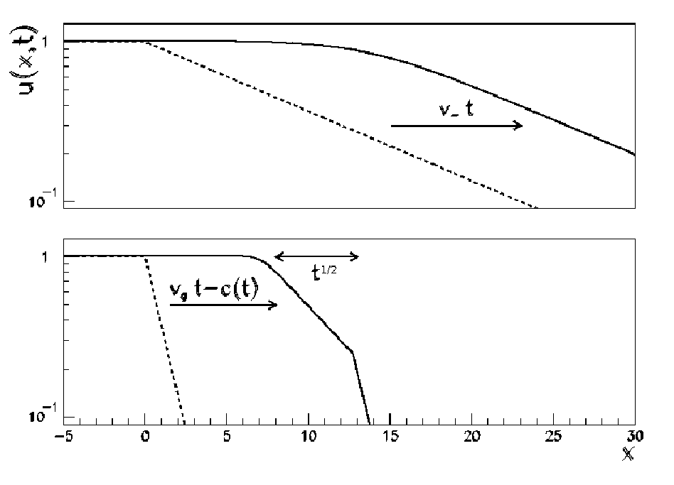
4.1.2 Diffusion equation with a boundary
We now come back to the original FKPP equation (119). We have seen that the nonlinearity has the effect of taming the growth induced by the linear term , when gets close to 1. But nonlinear partial differential equations are very difficult to address mathematically. It may be much simpler to address the linear equation
| (129) |
supplemented with an absorptive (moving with time) boundary condition that ensures that has a maximum value of at any time. We need to work out the solution of Eq. (129) with this kind of boundary condition. Here, we reformulate the approach proposed in the QCD context by Mueller and Triantafyllopoulos [35] (see also Ref. [102] for an account of the next-to-leading order BFKL kernel).
A solution to Eq. (129) with initial condition is given, for positive times, by
| (130) |
This solution holds if the boundary condition is at spatial infinity. The solution of the pure diffusion equation, without the growth term, is of course nothing but . We shall denote it by .

If instead of the boundary condition at infinity there is an absorptive barrier at say , i.e. if for any , then a solution may be found through a linear combination of the latter solution with different initial conditions, in such a way as the sum vanishes at . This is known as the method of images. It is based on the observation that any linear combination of Eq. (130) also solves Eq. (129). From the solution with initial condition , we subtract the solution of the same equation but with initial condition , in such a way that the solution vanishes for , at any time. We get
| (131) |
We do not expect the solution to this problem to represent accurately the solution to the full FKPP equation near the boundary . So the region of interest will be ahead of the boundary by a few units, while the starting point of the evolution is at some finite distance of the boundary:
| (132) |
One may then expand the two Gaussian terms:
| (133) |
The solution to the simple diffusion equation without the growth term, namely , is the one that we will actually use in the following. It would again be the latter solution scaled by , namely
| (134) |
where the superscript PD stands for “pure diffusion”. Note that in this equation, does not depend on time. We cannot implement in a straightforward way a time-dependent absorptive boundary. We will get to such a solution by successive iterations: The main trick is to go to a frame in which the solution of the branching diffusion with a boundary is stationary for large times.
Let us start from the solution in Eq. (130). The lines of constant (without a boundary) are obviously given by
| (135) |
(We have selected the rightmost solution ). Let us change frame by writing . Then in this new variable, in Eq. (130) reads
| (136) |
where we have factored out the solution of the pure diffusion equation, but this time, in the moving frame defined by the coordinate . We may implement an absorptive boundary condition, fixed in this new frame, by replacing by in Eq. (134). Note that is fixed with respect to , but in the original frame defined by coordinate , it is of order . The solution has lines of constant which solve
| (137) |
The two last terms are subdominant because according to Eq. (135), , and because is a constant. We further define a new frame
| (138) |
Going back to the expression for (see Eq. (130)), we substitute by its expression as a function of and get
| (139) |
We replace the expression inside the squared brackets, which is nothing but , by the solution with a boundary . We check that the value of for which is constant is now a mere constant for large . Going back to the original frame, we get
| (140) |
where
| (141) |
is the position of the absorptive boundary for large times, and thus, the position of the front. The constant is the position of the front in the moving frame. Setting and , the maximum of is reached at , and is indeed equal to 1.
For large or in the region which expands with time, the Gaussian factor goes to 1, and we see that only depends on one single variable . This was expected: It is precisely the defining property of traveling waves. But in addition to these asymptotic solutions, we get from this calculation the first finite- correction to the front shape and front velocity.
Actually, the speed of the front is intimately related to its shape. At time , it has reached its asymptotic shape over the distance from the saturation point. This remark will be important in the following.
We have derived the solution of a problem that was not exactly the initial one, however, we believe that the shape of the front in its forward part () as well as its velocity are quite universal. Indeed, physically, these properties are completely derived from the linear part of the equation. For this reason, the front is said to be “pulled” by its tail. The nonlinearity only tames the growth of near , and so its precise form should not influence the front position itself, at least at large enough times. Thus we expect these solutions to have a broad validity, only depending on the diffusion kernel, and so, may be obtainable from our calculation up to the replacement of the relevant parameters. For the more general branching diffusion kernel in Eq. (121), the velocity of the front would read
| (142) |
where solves , as was explained in Sec. 4.1.1. The front shape in its forward part reads
| (143) |
up to an overall constant. Fig. 19 represents a sketch of the solution at two different times. Note that the asymptotic shape is an exponential decay,
| (144) |
From Eq. (143), this shape extends over a range
| (145) |
In other words, the time needed for the front to reach its asymptotic shape over a range reads
| (146) |
Through our simple calculation, we got the lowest order in an expansion of the front shape and position at large times. The next corrections to would be of order 1 (this constant depends on the way we define the position of the front), followed by an algebraic series in whose terms all vanish at large . The first next-to-leading term in the series has been computed (see Ref. [103]): It turns out to be of order . We will not reproduce the calculations that lead to it because they are rather technical and there is already a comprehensive review paper available on the topic [72]. But let us write the result for the position and the shape of the front at that level of accuracy, for the more general branching diffusion kernel given by Eq. (121). To that accuracy, the front position reads [103]
| (147) |
For the simple FKPP case, we recall that , then and . The first two terms in the last equations match the ones found in Eq. (142). The shape of the front in its forward part has the following form:
| (148) |
where
| (149) |
and , are generalized hypergeometric functions. The terms in the first line match with the result of our calculation (Eq. (140)) for the relevant value of . These expressions should apply also to QCD, up to the relevant replacements given in Tab. 1.
So far, we have considered equations of the type of Eq. (119) as saturation equations, in the sense that they describe the diffusive growth of a continuous function until it is tamed for . We will see below that these equations may actually be given a different physical interpretation.
4.1.3 Discrete branching diffusion
We have investigated the solutions of the FKPP equation in a mathematical way, without discussing the physics that may lead to such an equation. The absorptive boundary that we have put replaces the nonlinear term in the FKPP equation, whose role is to make sure that never exceeds the limit . Hence we have thought of this boundary as a way to enforce the saturation of some density of particles. Actually, the FKPP equation (119) may stem from a branching diffusion process in which the number of particles is unlimited, and thus, for which there is no saturation at all. As a matter of fact, this is the way how the BK equation is built in QCD: An exponentially growing number of dipoles, stemming from the rapidity evolution of a hadronic probe, scatters off some target. The overall interaction probability is unitary because multiple scatterings are allowed (the interaction probability of dipoles is actually of the form ), but not because there is a saturation of the number of dipoles in the wavefunction of the probe. We refer the reader to Fig. 5 for a picture of the process.

To illustrate how the FKPP equation arises in such a simple model of branching diffusion, let us consider a set of particles on a line, each of them being indexed by a continuous variable . (Such a model was considered for instance in Ref. [71]). We let the system evolve according to the following rules. During the time interval , each particle has a probability to split in 2 particles. Unless it splits, it moves of the small random amount , which is a Gaussian random variable distributed like
| (150) |
Let us consider the number of particles contained in an interval of given size centered around the coordinate . At time , the system is supposed to consist in a single particle sitting at the origin . A sketch of a realization of this model is shown in Fig. 20. From the evolution rules, we easily get an equation for the average number of particles :
| (151) |
which reads, after replacing by Eq. (150) and after the limit has been taken,
| (152) |
All the dependence on the size of the “bin” is contained in the initial condition. It is clear that for large enough times, the solution to this equation is given by Eq. (130), and thus the lines of constant are given by Eq. (135).
Let us now define
| (153) |
where is some (large) constant. This definition is reminiscent of the -function, related to the scattering amplitude, introduced in the discussion of the BK equation in Sec. 2. For large enough , and thus . For any , the exponential makes sure that ranges between and . Thus (or ) has the shape of a traveling wave. Its position is the value of for which is some given constant say of the order of . Hence, up to fluctuations, it is given by Eq. (135).
On the other hand however, the average of over events, namely obeys the FKPP equation. Indeed
| (154) |
In the limit and rewriting the equation for , we get
| (155) |
Hence is a traveling wave at large times, and its position is given by Eq. (141). It is obviously behind by a term with respect to the value of for which the average number of particles has a given constant value. Furthermore, the probability distribution of the position of the rightmost particle (or of the -th rightmost particle for any given ) may also be derived from the FKPP equation. It turns out that in any event, the average for which has a given value, say , moves with the FKPP velocity which can be read off from Eq. (141). This is much slower than the velocity with which defined in such a way that moves.
All this may seem a bit paradoxical. But actually, it is just related to the fact that cannot be approximated by . We may understand it in the following way. By taking the average of , we have somewhat forgotten a fundamental property of : its discreteness. Indeed, it only takes integer values, and in particular, the distribution of in a realization has a finite support: At any time, there is a value of to the right of which there are no particles at all. obeys a stochastic equation. This is not the case for , which just obeys an ordinary branching diffusion equation.
In order to recover the effect of the discreteness of and compute the velocity, we may again use the absorptive boundary trick. Let us solve the linear equation
| (156) |
with an absorptive boundary. The absorptive boundary will be placed in such a way that at a distance of order one to its left (we will focus on the right-moving wave), (see Fig. 21). There is no difference in principle with the boundary calculation that we have performed before, except that the absorptive boundary is now placed to the right of the front (i.e. in the notations used above). Thus we find without any further calculation that the realizations of move, on the average, with the FKPP velocity (142).

4.2 Combining saturation and discreteness
We have seen that physically, the KPP equation (or the BK equation in QCD) may be interpreted either as an equation for the growth, diffusion and saturation of a continuous function, or as the evolution equation for the average of a bounded function of a discrete (thus stochastic) branching diffusion process. For each of these interpretations, we may find the main features of the solutions by imposing one absorptive boundary on the linear partial differential equation encoding branching diffusion. In one case, the boundary is a cutoff that prevents to be larger than 1: It represents saturation, i.e. the explicit nonlinearity present in the FKPP equation. In the other case, the boundary forces the function that represents the number of particles to vanish quickly when it becomes less than 1. Formally, it actually models the intrinsic discreteness of the number of particles, and avoids to address a stochastic equation directly.
In physical cases such as reaction-diffusion processes for finite , we define as the number of particles per site (or per bin) in normalized to . Hence it takes discrete values: , etc… While for large discreteness is unlikely to play a role in the region , it is expected to be crucial when . It is thus natural to impose the two boundaries: one representing saturation of the particle number, the other one discreteness of the same quantity. A model that these two cutoffs may represent is for example, the branching diffusion model in Sec. 4.1.3, but in which the total number of particles is limited to by keeping only the rightmost ones at each new branching. It is clear that the function defined to be the number of particles to the right of some position normalized to the maximum number is, for large enough times, a front connecting 1 (for ) to 0 (for ) (see Fig. 22).

Reaction-diffusion problems (described by nonlinear stochastic partial differential equations) were interpreted as branching diffusion problems taking place between two absorptive boundaries for the first time by Brunet and Derrida in Ref. [105] and, independently, by Mueller and Shoshi, in the case of QCD in Ref. [39]. Note however that the present interpretation of the cutoffs was only found in Ref. [40] in the context of the QCD parton model. Mueller and Shoshi considered both cutoffs for reasons related to the boost-invariance of the QCD amplitude. The duality of the two boundaries, that is to say of the dense and dilute regimes of the traveling wave, was studied more deeply in Refs. [106, 107, 108, 109, 110].
Before moving on to the technical derivation of the shape and position of the front in this case, let us figure out what we expect to find.
Starting from the initial condition, the front builds up and its velocity increases with (see Eq. (142)) until it reaches its asymptotic shape, which is a decreasing exponential that holds for all . But if the front is made of discrete particles, then it has a finite support, and the exponential shape may not extend to infinity to the right, since has to be either larger than , or zero. It cannot take values that would be a fraction of in realizations, and thus, we cannot accommodate the shape for arbitrarily large values of , since it would mean authorizing arbitrarily small positive values of . From Eq. (146) and from the shape of the asymptotic front (144), the exponential shape sets down to at time
| (157) |
Beyond, the front cannot develop any longer, and thus, its shape and velocity remain fixed. is the time that is needed for the front to relax from any perturbation, which is why we have put the subscript “relax”.
From Eq. (142) evaluated at , we get the new asymptotic velocity, that takes into account the effects of discreteness, in the form
| (158) |
The calculation of requires a proper account of the exact shape of the front. We shall turn to this calculation now.
As announced, we are now going to solve the linear branching diffusion equation with two absorptive boundaries: one representing saturation, the other one discreteness.

First, as in the one-boundary case, let us solve the simple diffusion equation between two boundaries, at and respectively, that is to say, with the conditions . The simplest method in this case is to take the ansatz
| (159) |
Then the diffusion equation reads
| (160) |
is necessarily a constant, being both a function of only and of only. The equations for and for are easily solved. All in all, we get for
| (161) |
where and are constants which we will shortly determine from the boundary condition. Note that only positive values of are physical, since negative ones would lead to an exponential increase of the solutions. The boundary conditions at and fix to and lead to a quantization of :
| (162) |
where is the size of the wave front and is an integer. The general solution is a sum of over all possible values of , with coefficients fixed by the initial condition. But at large time, thanks to the exponential decay of with , only the mode survives. The final solution thus reads
| (163) |
where the constant is determined from the projection of the initial condition on the fundamental mode of the “cavity” .
We now need to determine the time dependence of . It will follow from the search of the frame in which the front is stationary in time.
The first step (determination of , see Eq. (136)) is the same as in the one-boundary case. Starting from Eq. (136), we substitute with and look for the lines of constant . This leads us to introduce
| (164) |
Going back to the original variables, we get, for large,
| (165) |
where
| (166) |
We are left with the determination of the size of the front. Near the left boundary (at a distance of order 1), should be of order 1, while close to the right boundary, it should approach . We write
| (167) |
Then we see that and , where . The position of the rightmost boundary () is the point to the right of which there are no particles in typical individual realizations. We will denote it by .
4.3 Beyond the deterministic equations: Effect of the fluctuations
So far, we have actually solved deterministic equations although we were addressing a model with a discrete number of particles, that therefore has necessarily fluctuations. Our procedure gave the leading effects. We shall now incorporate more fluctuation effects, in a phenomenological way. (We shall essentially review Ref. [111]).
4.3.1 Phenomenological model and analytical results
The two-boundary procedure has led to the following result: The front propagates at a velocity in Eq. (170) lower than the velocity predicted by the mean-field equation (142), and its shape is the decreasing exponential down to the position
| (171) |
(up to a global constant independent of ) at which it is sharply cut off by an absorptive boundary. This boundary was meant to make the front vanish over one unit in , hence to implement discreteness on a deterministic equation.

But since the evolution is not deterministic, it may happen that a few extra particles are sent stochastically ahead of the tip of the front (See Fig. 24). Their evolution would pull the front forward. To model this effect, we assume that the probability per unit time that there be a particle sent at a distance ahead of the tip simply continues the asymptotic shape of the front, that is to say, the distribution of is
| (172) |
where is a constant. Heuristic arguments to support this assumption were presented in Ref. [111]. Note that while the exponential shape is quite natural since it is the continuation of the deterministic solution (143) in the linear regime, the fact that need to be strictly constant (and cannot be a slowly varying function of ) is a priori more difficult to argue.
Once a particle has been produced at position , say at time , it starts to multiply (see Fig. 24) and it eventually develops its own front (after a time of the order of ), that will add up to the deterministic primary front made of the evolution of the bulk of the particles.
Note that the philosophy of our phenomenological approach to the treatment of the fluctuations is identical to the spirit of the statistical approach in Sec. 3.3 developped for the zero-dimensional model. Whenever the number of particles is larger than ( here), we apply a deterministic nonlinear evolution. Fluctuations instead are produced with a probability which stems from a linear equation.
Let us estimate the shift in the position of the front induced by these extra forward particles. Between the times (of the order of 1) and , the velocity of the secondary front is given by Eq. (142). Hence its position , after relaxation, will be given by
| (173) |
where . Eq. (173) holds up to a constant independent of and . We have used Eq. (142) to express . The observed front will eventually result in the sum of the primary and secondary fronts, after relaxation of the latter. Its position will be supplemented by a shift that may be computed by writing the resulting front shape in the large- tail as the sum of the primary and secondary fronts:
| (174) |
where is an undetermined constant. From Eq. (174) we get the shift
| (175) |
The probability distribution (172) and the front shift (175) due to a forward fluctuation define an effective theory for the evolution of the position of the front :
| (176) |
From these rules, we may compute all cumulants of , by writing the evolution of their generating function, deduced from the effective theory (176):
| (177) |
The left hand-side is a power series in whose coefficients are the time derivatives of the cumulants of . Identifying the powers of in the left and right handside, we get
| (178) |
We see that the statistics of the position of the front still depend on the product of the undetermined constants and . We need a further assumption to fix its value.
We go back to the expression for the correction to the mean-field front velocity, given in Eq. (170). From the expressions of (Eq. (175)) and of (Eq. (172)), we see that the integrand defining in Eq. (178) is almost a constant function of for , and is decaying exponentially for . Furthermore, is of order 1, which means that when a fluctuation is sent out at a distance ahead of the tip of the front, it evolves into a front that matches in position the deterministic primary front. We also notice that when a fluctuation has , its evolution is completely linear until it is incorporated to the primary front, whereas fluctuations with evolve nonlinearly but at the same time have a very suppressed probability. We are thus led to the natural conjecture that the average front velocity is given by in Eq. (170), with the replacement
| (179) |
namely
| (180) |
The large- expansion of the new expression of the velocity yields a correction of the order of to the Brunet-Derrida result, more precisely
| (181) |
Eqs. (178) and (181) match for the choice . From this determination of , we also get the full expression of the cumulants of the position of the front:
| (182) |
We note that all cumulants are of order unity for , which is the sign that the distribution of the front position is far from being a trivial Gaussian. This makes it particularly interesting. On the other hand, the cumulants are proportional to , which is the sign that the position of the front is the result of the sum of independent random variables, and as such, becomes Gaussian when is very large. The properties of the statistics of the front position were investigated in some more details in Ref. [112].
4.3.2 Numerical simulations
These results rely on a number of conjectures that no-one has been able to prove so far. In order to check our results, let us consider again the model introduced in Sec. 2.2.2. The first step to take before being able to apply our results to this particular model is to extract from the linear part of Eq. (23) the corresponding function , and then to compute . Setting , we get
| (183) |
and is defined by .
For the purpose of our numerical study, we set
| (184) |
Simulated realizations for this set of parameters are shown in Fig. 25.
From (183), this choice leads to
| (185) |
Predictions for all cumulants of the position of the front are obtained by replacing the values of these parameters in Eqs. (181),(182).
Technically, in order to be able to go to very large values of , we replace the full stochastic model by its deterministic mean field approximation , where the evolution of is given by Eq. (23), in all bins in which the number of particles is larger than (that is, in the bulk of the front). Whenever the number of particles is smaller, we use the full stochastic evolution (21). We add an appropriate boundary condition on the interface between the bins described by the deterministic equation and the bins described by the stochastic equation so that the flux of particles is conserved [113]. This setup will be called “model I”. Eventually, we shall use the mean field approximation everywhere except in the rightmost bin (model II): at each time step, a new bin is filled immediately on the right of the rightmost nonempty site with a number of particles given by a Poisson law of average We checked numerically that this last approximation gives indistinguishable results from those obtained within model I as far as the statistics of the position of the front is concerned.
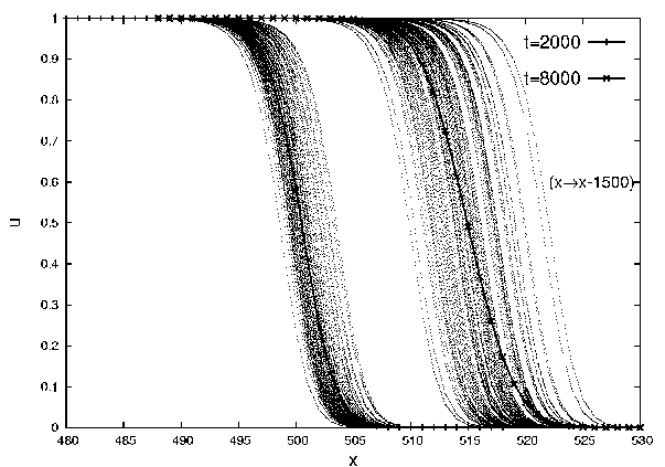
We define the position of the front at time by
| (186) |
We start at time from the initial condition for and for . We evolve it up to time to get rid of subasymptotic effects related to the building up of the asymptotic shape of the front, and we measure the mean velocity between times and . For model I (many stochastic bins), we average the results over such realizations. For model II (only one stochastic bin), we generate such realizations for and realizations for . In all our simulations, models I and II give numerically indistinguishable results for the values of where both models were simulated, as can be seen on the figures (results for model I are represented by a circle and for model II by a cross).
Our numerical data for the cumulants is shown in Fig. 26 together with the analytical predictions obtained from (181),(182) (dotted lines in the figure). We see that the numerical simulations get very close to the analytical predictions at large . However, higher-order corrections are presumably still important for the lowest values of displayed in the figure.

We try to account for these corrections by replacing the factor in the denominator of the expression for the cumulants in Eqs. (181),(182) by the ansatz
| (187) |
The two first terms in the r.h.s. are suggested by our model. We have added two subleading terms which go beyond our theory: a constant term, and a term that vanishes at large . The latter are naturally expected to be among the next terms in the asymptotic expansion for large . We include them in this numerical analysis because in the range of in which we are able to perform our numerical simulations, they may still bring a significant contribution.
We fit (187) to the numerical data obtained in the framework of model II, restricting ourselves to values of larger than . In the fit, each data point is weighted by the statistical dispersion of its value in our sample of data. We obtain a determination of the values of the free parameters and , with a good quality of the fit ().
Now we see that with this modification, the results for the cumulants shown in figure 26 (full lines), are in excellent agreement with the numerical data over the whole range of .
5 Application to the computation of QCD scattering amplitudes
In this section, we shall study the phenomenological relevance of the results obtained from the correspondence with statistical physics. There are two aspects that should be discussed. First, we go back to the assumptions that were required to go from QCD to reaction-diffusion, and in particular, the hypothesis of uniformity of the evolution in impact-parameter space. Next, we derive new properties of the QCD scattering amplitudes and discuss their impact on phenomenology.
5.1 Relevance of one-dimensional models: impact-parameter correlations
So far, we have argued that high-energy scattering in QCD at fixed coupling and fixed impact parameter is in the universality class of the stochastic FKPP equation (Sec. 2), which is an equation with one evolution variable (time or rapidity in QCD), and one spatial dimension ( generically, or in QCD). From the very beginning, we have simply discarded the impact parameter dependence. It is important to understand that the spatial variable and the impact parameter play different roles, and thus, the impact parameter may a priori not be accounted for by a two-dimensional extension of the FKPP equation.
There are general arguments to support the assumption that the QCD evolution is local enough in impact parameter for the different impact parameters to decouple through the rapidity evolution, which we are now going to present.
Let us start with a single dipole at rest, and bring it gradually to a higher rapidity. As was explained in Sec. 2, during this process, this dipole may be replaced by two new dipoles, which themselves may split, and so on, eventually producing a chain of dipoles. Figure 3 pictures one realization of such a chain.
According to the splitting rate given in Eq. (1), splittings to smaller-size dipoles are favored, and thus, one expects that the sizes of the dipoles get smaller on the average, and that in turn, the successive splittings become more local. The dipoles around region “1” and those around region “2” should have an independent evolution beyond the stage pictured in Fig. 3: further splittings will not mix in impact parameter space, and thus, the traveling waves around these regions should be uncorrelated. For a dipole in region 1 of size to migrate to region 2, it should first split into a dipole whose size is of the order of the distance between regions 1 and 2, up to some multiplicative factor of order . (We assume in this discussion that the dipoles in region 2 relevant to the propagation of the local traveling waves, that is, those which are in the bulk of the wave front, also have sizes of order ). Roughly speaking, the rate of such splittings may be estimated from the dipole splitting probability (1): it is of order , while the rate of splittings of the same dipole into a dipole of similar size in region 1 is of order . Thus the first process is strongly suppressed as soon as regions 1 and 2 are more distant than a few units of . Note that for , saturation may further reduce the emission of the first, large, dipole leading to an even stronger suppression of the estimated rate.
What could also happen is that some larger dipole has, by chance, one of its endpoints tuned to the vicinity of the coordinate one is looking at (at a distance which is at most ), and easily produces a large number of dipoles there. In this case, the position of the traveling wave at that impact parameter would suddenly jump. If such events were frequent enough, then they would modify the average wave velocity and thus the one-dimensional sFKPP picture. We may give a rough estimate of the rate at which dipoles of size smaller than are produced. Assuming local uniformity for the distribution of the emitting dipoles, the rate (per unit of ) of such events can be written
| (188) |
where we integrate over large dipoles of size emitting smaller dipoles (of size ) with a probability . The factor accounts for the fact that one endpoint of the dipole of size has to be in a given region of size in order to emit the dipoles at the right impact parameter. To estimate this expression, we first use and approximate by
| (189) |
The front is replaced by 1 above the saturation scale (for ) and by an exponentially decaying tail for . Using in the emission kernel, the integration is then easily performed and one finds a rate whose dominant term is
| (190) |
For , i.e. ahead of the bulk of the front, this term is parametrically less than 1 and is in fact of the order of the probability to find an object in this region that contributes to the normal evolution of the front [111]. Hence there is no extra contribution due to the fact that there are many dipoles around at different impact parameters.
The arguments given here are based on estimates of average numbers of dipoles, on typical configurations, and we are not able to account analytically for the possible fluctuations. As we have seen through this review, the latter often play an important role. As a matter of fact, in the physics of disordered systems, rare events sometimes dominate. So before studying the phenomenological consequences of the statistical picture of high-energy QCD based on a one-dimensional equation, one should check more precisely locality of the evolution in impact parameter.
A numerical check was recently achieved in the case of a toy model that has an impact-parameter dependence in Ref. [114]. Let us briefly describe the model.
5.1.1 A model incorporating an impact-parameter dependence
In order to arrive at a model that is tractable numerically, we only keep one transverse dimension instead of two in 3+1-dimensional QCD. However, we cannot consider genuine 2+1-dimensional QCD because we do not wish to give up the logarithmic collinear singularities at and . Moreover, QCD with one dimension less has very different properties at high energies [115]. Starting from Eq. (1), a splitting rate which complies with our requirements is:
| (191) |
We can further simplify this probability distribution by keeping only its collinear and infrared asymptotics (as in Ref. [116]). If (or the symmetrical case ), the probability reduces to ( resp.). The result of the splitting is a small dipole together with one close in size to the parent. So for simplicity we will just add the small dipole to the system and leave the parent unchanged. In the infrared region, a dipole of size is emitted with a rate given by the large- limit of the above probability. The probability laws (1),(191) imply that a second dipole of similar size should be produced while the parent dipole disappears. To retain a behavior as close as possible to that in the collinear limit, we will instead just generate a single large dipole and maintain the parent. To do this consistently one must include a factor of two in the infrared splitting rate, so as not to modify the average rate of production of large dipoles.
In formulating our model precisely, let us focus first on the distribution of the sizes of the participating dipoles. (The simplifying assumptions made above enable one to choose the sizes and the impact parameters of the dipoles successively). We call the modulus of the emitted dipole, the modulus of its parent and . The splitting rate (191) reads, in this simplified model
| (192) |
and the original parent dipole is kept. Logarithmic variables are the relevant ones here, so we introduce
| (193) |
We can thus rewrite the dipole creation rate as
| (194) |
To further simplify the model, we discretise the dipole sizes in such a way that is now an integer. This amounts to restricting the dipole sizes to negative integer powers of . The probability that a dipole at lattice site (i.e. a dipole of size ) creates a new dipole at lattice site is
| (195) |
The rates for a dipole at lattice site to split to any lattice site or respectively are then given by
| (196) |
where we have restricted the lattice to , for obvious reasons related to the numerical implementation.
Now we have to address the question of the impact parameter of the emitted dipole. In QCD, the collinear dipoles are produced near the endpoints of the parent dipoles. Let us take a parent of size at impact parameter . We set the emitted dipole (size ) at the impact parameter such that
| (197) |
where has uniform probability between 0 and 1. It is introduced to obtain a continuous distribution of the impact parameter unaffected by the discretisation of . This prescription is quite arbitrary in its details, but the latter do not influence significantly the physical observables. Each of the two signs that appear in the above expression is chosen to be either or with equal weights. We apply the same prescription when the emitted dipole is larger than its parent.
Scattering amplitude
We have explained above (see Sec. 2.1) that in QCD, the scattering amplitude of an elementary probe dipole of size with a dipole in an evolved Fock state is proportional to the number of objects which have a size of the same order of magnitude and which sit in a region of size of order around the impact point of the probe dipole. Since in our case, the sizes are discrete, the amplitude is just given, up to a factor, by the number of dipoles that are exactly in the same bin of size as the probe, namely
| (198) |
Saturation
We now have to enforce unitarity, that is the condition
| (199) |
for any and . This condition is expected to hold due to gluon saturation in QCD. However, saturation is not included in the original dipole model. The simplest choice is to veto splittings that would locally drive the amplitude to values larger than 1. In practice, for each splitting that gives birth to a new dipole of size at impact parameter , we compute and , and throw away the produced dipole whenever one of these numbers gets larger than one.
Given the definition of the amplitude , this saturation rule implies that there is a maximum number of objects in each bin of size and at each impact parameter, which is equal to .
5.1.2 Numerical results
We take as an initial condition a number of dipoles of size 1 (), uniformly distributed in impact parameter between and . The impact parameters that are considered are respectively , , , and . The number of events generated is typically ,which allows one to measure the mean and variance of the position of the traveling waves to a sufficient accuracy.
We have checked that at each impact parameter, we get traveling waves whose positions grow linearly with rapidity at a velocity less than the expected mean-field velocity for this model. was varied from 10 to 200.
Fig. 27 represents the correlations between the positions of the wave fronts at different impact parameters in the AIP model, defined as
| (200) |
We set to 25 in that figure, but we also repeated the analysis for different values of between 10 and 200.
We see very clearly the successive decouplings of the different impact parameters in Fig. 27, from the most distant to the closest one, as rapidity increases. Indeed, the correlation functions flatten after some given rapidity depending on the difference in the probed impact parameters, which means that the evolutions decouple. This decoupling is expected as soon as the traveling wave front reaches dipole sizes which are smaller than the distance between the probed impact parameters, i.e. at such that . From the data for , we can estimate quantitatively the values of the rapidities at which the traveling waves decouple between the different impact parameters. (It is enough to invert the above formula for the relevant values of ). These rapidities are denoted by a cross in Fig. 27 for the considered impact parameter differences. Our numerical results for the correlations are nicely consistent with this estimate, since the correlations start to saturate to a constant value precisely on the right of each such cross.
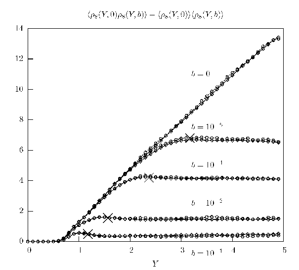
We conclude that the different impact parameters indeed decouple, as was expected from a naive analytical estimate. What is true for our toy model should go over to full QCD, since we have included the main features of QCD. When looking at the numerical data more carefully however, it turns out that the model with impact parameter does not reduce exactly to a supposedly equivalent one-dimensional model of the sFKPP type. This is a point that would deserve more work. We refer the reader to Ref. [114] for all details of our numerical investigations.
An attempt to build a complete picture of high-energy QCD that includes the impact parameter was made in Ref. [117], but it relies on some more conjectures, that are difficult to prove. Finding a mathematically sound formulation remains a challenge.
5.2 Traveling waves, geometric scaling, and consequences of the noise
As was stated in the Introduction, the initially unplanned opportunity to collect data in the high-energy regime of deep-inelastic scattering at HERA triggered a renewed interest in small- physics among phenomenologists. The major discoveries in this regime is the (unexpected) important fraction of diffractive events, and a new scaling, geometric scaling, featured by total (and even semi-inclusive) cross sections (see Fig. 1).
In order to deal theoretically with the small- regime, one needs new factorization theorems in order to single out the elements of the cross sections that are computable in perturbation theory. High-energy, or -factorization, [118, 119, 120] is the appropriate tool. A practical way to implement -factorization is the color dipole model presented in Sec. 2.
5.2.1 Dipole models and geometric scaling
The main observable measured at HERA is the proton structure function . It is proportional to the sum of the virtual photon-proton cross section for a transversely and longitudinally polarized photon respectively.
A bare photon has no hadronic interactions, since it does not carry any color charge. However, it may easily fluctuate into a quark-antiquark pair, overall color-neutral, thus forming a color dipole. Subsequently, these dipoles will interact with the target proton. This picture is represented by the following equations:
| (201) |
Here, are the photon-proton cross sections for transversly and longitudinally polarized virtual photons. are light-cone wavefunctions for , computable within QED (see, e.g., Ref. [27] for explicit expressions to lowest order in ). Furthermore, is the cross-section for dipole–proton scattering (for a dipole of transverse size ), and encodes all the information about hadronic interactions (including unitarization effects). This cross section is related to the amplitude discussed so far by an integration over the impact parameter. (Actually, was the forward elastic amplitude; the optical theorem relates it to the total cross section).
In Ref. [27, 28], the dipole cross-section was modeled as
| (202) |
where is a hadronic cross-section: It stems from the integration over the impact parameter, when the impact parameter dependence is supposed to be uniform over a disk of radius . plays the role of the saturation momentum, parametrized as GeV2. Note that, by construction, this cross section only depends on the combined variable instead of and separately. This property is transmitted to the measured photon cross sections , which then depend on only (this scaling is slightly violated by the masses of the quarks). This is geometric scaling, predicted to be a feature of the solutions to the BK equation at large rapidity.
Historically, geometric scaling was discovered first in the data (see Ref. [29]), after Golec-Biernat and Wüsthoff (GBW) had written down their model: The latter happened to feature this scaling (up to small violations induced by the quark masses). There was no apparent need for finite rapidity scaling violations in the first HERA data. However, later analysis revealed that a significant amount of explicit scaling violations in the dipole cross section, predicted by the BK equation, were actually required by more accurate data.
A now popular model that describes the HERA data in a way that takes a better account of the subasymptotics, beyond the GBW model, was formulated in Ref. [121]. The dipole scattering cross section reads , with
| (203) |
where GeV. The expression for the cross section for small compared to corresponds to the solution of the BK equation (compare to Eq. (143) with the help of Tab. 1), in which we substituted and by the parameters and that we subsequently fit to the data. The expression in the second line also has the correct functional form for , as obtained by solving the BK equation [32]. This is strictly valid only to leading-order accuracy, but here it is used merely as a convenient interpolation towards the ‘black disk’ limit . (The details of this interpolation are unimportant for the calculation of .) The coefficients and are determined uniquely from the condition that and its slope be continuous at . The overall factor in the first line of Eq. (203) is ambiguous, reflecting an ambiguity in the definition of . This model fits well all HERA data for structure functions, in the range . All details may be found in Ref. [121].
The model explicitely breaks geometric scaling. However, effectively, geometric scaling remains a fairly good symmetry of the model, as required by the data. The small finite-rapidity scaling violations are needed to describe accurately the high-precision HERA data.
The model may also accomodate less inclusive observables, such as diffraction [122]. It has been improved recently by including heavy quarks [123] (The crucial need for taking account of the charm quark was emphasized in Ref. [124]). An impact-parameter dependence was also introduced [125, 126, 127] that was already missing in the GBW model.
The range of validity of dipole models has been re-examined recently [128].
5.2.2 Diffusive scaling
At still higher energies, according to the discussion of Sec. 4, one expects the saturation scale to acquire a dispersion from event to event that scales with the rapidity like when rapidity increases. Although this dispersion is not an observable since there is no way to measure the saturation scale of an individual event, it manifests itself in the total cross section in the form of a new scaling, different from geometric scaling.
The physical amplitude for the scattering of a dipole of size off some target is given by the average of all realizations of the evolution at a given :
| (204) |
For large enough rapidities and small enough , these realizations are exponentially decaying fronts in the variable , fully characterized by a stochastic saturation scale, or rather its logarithm . For the purpose of the present discussion, it may be approximated in the same way as in Eq. (189), namely
| (205) |
The statistics of is given by Eqs. (181),(182) (up to the replacements suggested in Tab. 1 to go from a generic reaction-diffusion to QCD). At ultrahigh energies (and very small ), it is essentially a Gaussian centered at
| (206) |
and of variance
| (207) |
The scattering amplitude may be expressed by the simple formula
| (208) |
The most remarkable feature of this amplitude is the scaling form for that it yields:
| (209) |
This equation may be obtained by performing the integration in Eq. (208) after the replacement of by its approximation (205). This scaling obviously violates geometric scaling: If the latter scaling were satisfied, then would be a function of only.
Mueller and Shoshi had already noted that geometric scaling had to be violated beyond the BK equation in Ref. [39]. However, the square root in the denominator of the scaling variable in Eq. (209) was missing because their approach was relying on mean field throughout, thus missing the stochastic nature of the evolution.
This new scaling is a firm prediction of the correspondence with statistical physics. However, it may not be tested at particle colliders in a simple way. Let us work out the order of magnitude of the rapidity needed for the different effects (saturation, geometric scaling, diffusive scaling) to show up. The rapidity that is needed to reach saturation is roughly
| (210) |
The BK picture is expected to be valid until the asymptotic exponential shape of the front has diffused down to the point where the amplitude becomes of the order of . This additional rapidity needed to get to the regime of geometric scaling is thus given by Eq. (157) once the appropriate replacements have been done
| (211) |
and finally, the effect of the fluctuations of the saturation scale gets important at the rapidity
| (212) |
The relevant parameters read, in QCD,
| (213) |
For some realistic strong coupling constant, , we get
| (214) |
Given that rapidities in the small- regime at HERA were of the order of 10, and will be of the order of 15 at the LHC, these figures may give us the hope that we may observe these effects. However, the values of the rapidity that delimitates the different regimes are largely underestimated given that they rely on the leading-order BFKL kernel, which predicts a much too large growth of the cross section with the rapidity and a too fast diffusion (see the large value of ). One also has to keep in mind that the former estimates should only hold for very small values of .
Furthermore, the effect of the running coupling, which should be taken into account in any detailed phenomenological study, is expected to still reduce the effects of the fluctuations [129].
Nevertheless, the effect of diffusive scaling (i.e. of the event-by-event fluctuations of the saturation scale) on observables has already been investigated in some detail by several groups. Diffractive amplitudes were studied in Ref. [130]. The ratio of the gluon distribution in a nucleus to the same quantity in a proton was computed in Ref. [131].
6 Conclusion and outlook
We have reviewed a peculiar way of viewing high-energy scattering in QCD, based on the physics of the parton model, and its strong similarities with reaction-diffusion processes (Sec. 2). The correspondence is best summarized in the mapping of Tab. 1. We have seen that the equations that describe the dynamics of these processes are in the universality class of the stochastic FKPP equation, and admit traveling-wave solutions whose features are likely to be universal, in such a way that a study of simple reaction-diffusion-like models may lead to exact asymptotic results also for QCD scattering amplitudes. Understanding the very mechanism of traveling wave formation and front propagation was crucial to see how the universality may come about (see Sec. 4).
In zero-dimensional stochastic models, we could perform exact calculations and get analytical results within different formulations (Sec. 3). We understood that analyzing the structure of single events was technically much simpler if one wants to get leading orders at large (), since in individual realizations, one may factorize the fluctuating part from the nonlinear effects. Thanks to this observation, in one-dimensional models which admit realizations in the form of stochastic traveling waves, we could also get precise analytical results on the form and shape of the traveling waves, which are presumably exact asymptotically (Sec. 4). Universality enables one to make statements on the form of the QCD scattering amplitudes at very high energies. These statements turn into firm phenomenological predictions (Sec. 5), which however do not seem to be testable at colliders in the near future. Nevertheless, getting new analytical results for QCD in some limit is always an interesting achievement, given the complexity of the theory. Furthermore, while our analytical results only apply for exponentially small (), the picture itself should be valid in the whole perturbative range, namely for .
There are still many open questions. On the statistical physics side, the statistics of the front position that we have found has not been derived rigorously, but rather guessed, and rely on many quite ad hoc conjectures. We got confidence on the validity of our conjectures on the basis of numerical simulations. Moreover, although we expect universality up to corrections of order (that is to say in QCD), we could only get analytical expressions relative to the cumulants of the position of the front for the first terms in an expansion in powers of , which requires much larger values of to be valid. On a more general footing, the sFKPP equation seems to describe many physical, chemical or biological problems (in particular population evolution with selection in evolutionary biology). We have also found recently an explicit analogy with the theory of spin glasses [132]. This large universality is maybe the strongest incentive to try and find more accurate solutions to that kind of equations.
On the QCD side, the correspondence with reaction-diffusion processes strongly relies on the assumption that there is saturation of some form of the quark and gluon densities in the hadronic wave functions. While this is a reasonable guess that few experts would challenge, it is clear that we cannot consider that the problem is solved before the saturation mechanism at work in QCD has been exhibited. QCD is formulated as a quantum field theory. To see the similarity with reaction-diffusion, we basically needed to translate it into the parton model first. It would be better to recover the results of Sec. 4 (and hopefully get more) directly from field theory [133], as one could do it in the zero-dimensional model introduced in Sec. 3. This requires to understand the strong field regime of field theory. This is an exciting challenge for both particle physicists and statistical physicists.
Acknowledgements
I thank Dr Urko Reinosa for his reading of the manuscript and his helpful comments. This work was supported in part by the Agence Nationale de la Recherche (France), contract ANR-06-JCJC-0084-02.
References
- [1] T. Muta, Foundations of quantum chromodynamics. Second edition, World Sci. Lect. Notes Phys. 57 (1998) 1–409.
- [2] V. N. Gribov, L. N. Lipatov, Deep inelastic e p scattering in perturbation theory, Sov. J. Nucl. Phys. 15 (1972) 438–450.
- [3] Y. L. Dokshitzer, Calculation of the Structure Functions for Deep Inelastic Scattering and e+ e- Annihilation by Perturbation Theory in Quantum Chromodynamics. (In Russian), Sov. Phys. JETP 46 (1977) 641–653.
- [4] G. Altarelli, G. Parisi, Asymptotic Freedom in Parton Language, Nucl. Phys. B126 (1977) 298.
- [5] L. N. Lipatov, Reggeization of the Vector Meson and the Vacuum Singularity in Nonabelian Gauge Theories, Sov. J. Nucl. Phys. 23 (1976) 338–345.
- [6] E. A. Kuraev, L. N. Lipatov, V. S. Fadin, The Pomeranchuk Singularity in Nonabelian Gauge Theories, Sov. Phys. JETP 45 (1977) 199–204.
- [7] I. I. Balitsky, L. N. Lipatov, The Pomeranchuk Singularity in Quantum Chromodynamics, Sov. J. Nucl. Phys. 28 (1978) 822–829.
- [8] M. Ciafaloni, G. Camici, Energy scale(s) and next-to-leading BFKL equation, Phys. Lett. B430 (1998) 349–354.
- [9] V. S. Fadin, L. N. Lipatov, BFKL pomeron in the next-to-leading approximation, Phys. Lett. B429 (1998) 127–134.
- [10] L. D. McLerran, The color glass condensate and small x physics: 4 lectures, Lect. Notes Phys. 583 (2002) 291–334.
- [11] E. Iancu, R. Venugopalan, The color glass condensate and high energy scattering in QCD.
- [12] L. V. Gribov, E. M. Levin, M. G. Ryskin, Singlet Structure Function at Small x: Unitarization of Gluon Ladders, Nucl. Phys. B188 (1981) 555–576.
- [13] L. V. Gribov, E. M. Levin, M. G. Ryskin, Semihard Processes in QCD, Phys. Rept. 100 (1983) 1–150.
- [14] A. H. Mueller, J.-w. Qiu, Gluon Recombination and Shadowing at Small Values of x, Nucl. Phys. B268 (1986) 427.
- [15] L. D. McLerran, R. Venugopalan, Computing quark and gluon distribution functions for very large nuclei, Phys. Rev. D49 (1994) 2233–2241.
- [16] L. D. McLerran, R. Venugopalan, Gluon distribution functions for very large nuclei at small transverse momentum, Phys. Rev. D49 (1994) 3352–3355.
- [17] L. D. McLerran, R. Venugopalan, Green’s functions in the color field of a large nucleus, Phys. Rev. D50 (1994) 2225–2233.
- [18] I. Balitsky, Operator expansion for high-energy scattering, Nucl. Phys. B463 (1996) 99–160.
- [19] J. Jalilian-Marian, A. Kovner, A. Leonidov, H. Weigert, The BFKL equation from the Wilson renormalization group, Nucl. Phys. B504 (1997) 415–431.
- [20] J. Jalilian-Marian, A. Kovner, A. Leonidov, H. Weigert, The Wilson renormalization group for low x physics: Towards the high density regime, Phys. Rev. D59 (1998) 014014.
- [21] E. Iancu, A. Leonidov, L. D. McLerran, The renormalization group equation for the color glass condensate, Phys. Lett. B510 (2001) 133–144.
- [22] E. Iancu, A. Leonidov, L. D. McLerran, Nonlinear gluon evolution in the color glass condensate. I, Nucl. Phys. A692 (2001) 583–645.
- [23] H. Weigert, Unitarity at small Bjorken x, Nucl. Phys. A703 (2002) 823–860.
- [24] Y. V. Kovchegov, Small-x F2 structure function of a nucleus including multiple pomeron exchanges, Phys. Rev. D60 (1999) 034008.
- [25] Y. V. Kovchegov, Unitarization of the BFKL pomeron on a nucleus, Phys. Rev. D61 (2000) 074018.
- [26] A. H. Mueller, Soft gluons in the infinite momentum wave function and the BFKL pomeron, Nucl. Phys. B415 (1994) 373–385.
- [27] K. J. Golec-Biernat, M. Wusthoff, Saturation effects in deep inelastic scattering at low Q**2 and its implications on diffraction, Phys. Rev. D59 (1999) 014017.
- [28] K. J. Golec-Biernat, M. Wusthoff, Saturation in diffractive deep inelastic scattering, Phys. Rev. D60 (1999) 114023.
- [29] A. M. Stasto, K. J. Golec-Biernat, J. Kwiecinski, Geometric scaling for the total gamma* p cross-section in the low x region, Phys. Rev. Lett. 86 (2001) 596–599.
- [30] C. Marquet, L. Schoeffel, Geometric scaling in diffractive deep inelastic scattering, Phys. Lett. B639 (2006) 471–477.
- [31] E. Levin, K. Tuchin, Solution to the evolution equation for high parton density QCD, Nucl. Phys. B573 (2000) 833–852.
- [32] E. Levin, K. Tuchin, New scaling at high energy DIS, Nucl. Phys. A691 (2001) 779–790.
- [33] N. Armesto, M. A. Braun, Parton densities and dipole cross-sections at small x in large nuclei, Eur. Phys. J. C20 (2001) 517–522.
- [34] K. J. Golec-Biernat, L. Motyka, A. M. Stasto, Diffusion into infra-red and unitarization of the BFKL pomeron, Phys. Rev. D65 (2002) 074037.
- [35] A. H. Mueller, D. N. Triantafyllopoulos, The energy dependence of the saturation momentum, Nucl. Phys. B640 (2002) 331–350.
- [36] R. A. Fisher, Ann. Eugenics 7 (1937) 355.
- [37] A. Kolmogorov, I. Petrovsky, N. Piscounov, Moscou Univ. Bull. Math. A1 (1937) 1.
- [38] S. Munier, R. B. Peschanski, Geometric scaling as traveling waves, Phys. Rev. Lett. 91 (2003) 232001.
- [39] A. H. Mueller, A. I. Shoshi, Small-x physics beyond the Kovchegov equation, Nucl. Phys. B692 (2004) 175–208.
- [40] E. Iancu, A. H. Mueller, S. Munier, Universal behavior of QCD amplitudes at high energy from general tools of statistical physics, Phys. Lett. B606 (2005) 342–350.
- [41] N. N. Nikolaev, B. G. Zakharov, Colour transparency and scaling properties of nuclear shadowing in deep inelastic scattering, Z. Phys. C49 (1991) 607–618.
- [42] N. Nikolaev, B. G. Zakharov, Pomeron structure function and diffraction dissociation of virtual photons in perturbative QCD, Z. Phys. C53 (1992) 331–346.
- [43] C. Ewerz, O. Nachtmann, Towards a Nonperturbative Foundation of the Dipole Picture: I. Functional Methods, Annals Phys. 322 (2007) 1635–1669.
- [44] C. Ewerz, O. Nachtmann, Towards a Nonperturbative Foundation of the Dipole Picture: II. High Energy Limit, Annals Phys. 322 (2007) 1670–1726.
- [45] L. N. Lipatov, The Bare Pomeron in Quantum Chromodynamics, Sov. Phys. JETP 63 (1986) 904–912.
- [46] I. Balitsky, Factorization for high-energy scattering, Phys. Rev. Lett. 81 (1998) 2024–2027.
- [47] I. Balitsky, Factorization and high-energy effective action, Phys. Rev. D60 (1999) 014020.
- [48] R. A. Janik, R. B. Peschanski, QCD saturation equations including dipole-dipole correlation, Phys. Rev. D70 (2004) 094005.
- [49] R. A. Janik, QCD saturation in the dipole sector with correlations, Phys. Lett. B604 (2004) 192–198.
- [50] E. Levin, M. Lublinsky, Balitsky’s hierarchy from Mueller’s dipole model and more about target correlations, Phys. Lett. B607 (2005) 131–138.
- [51] K. Rummukainen, H. Weigert, Universal features of JIMWLK and BK evolution at small x, Nucl. Phys. A739 (2004) 183–226.
- [52] Z. Chen, A. H. Mueller, The Dipole picture of high-energy scattering, the BFKL equation and many gluon compound states, Nucl. Phys. B451 (1995) 579–604.
- [53] Y. V. Kovchegov, A. H. Mueller, S. Wallon, Unitarity corrections and high field strengths in high energy hard collisions, Nucl. Phys. B507 (1997) 367–378.
- [54] A. H. Mueller, G. P. Salam, Large multiplicity fluctuations and saturation effects in onium collisions, Nucl. Phys. B475 (1996) 293–320.
- [55] E. Avsar, G. Gustafson, L. Lonnblad, Energy conservation and saturation in small-x evolution, JHEP 07 (2005) 062.
- [56] E. Avsar, G. Gustafson, L. Lonnblad, Small-x dipole evolution beyond the large-N(c) limit, JHEP 01 (2007) 012.
- [57] A. H. Mueller, Parton saturation: An overview, arxiv:hep-ph/0111244.
- [58] A. H. Mueller, Small x Behavior and Parton Saturation: A QCD Model, Nucl. Phys. B335 (1990) 115.
- [59] A. H. Mueller, Parton saturation at small x and in large nuclei, Nucl. Phys. B558 (1999) 285–303.
- [60] J. R. Forshaw, D. A. Ross, Quantum chromodynamics and the pomeron, Cambridge Lect. Notes Phys. 9 (1997) 1–248.
- [61] R. Kirschner, L. N. Lipatov, L. Szymanowski, Effective action for multi - Regge processes in QCD, Nucl. Phys. B425 (1994) 579–594.
- [62] R. Kirschner, L. N. Lipatov, L. Szymanowski, Symmetry properties of the effective action for high- energy scattering in QCD, Phys. Rev. D51 (1995) 838–855.
- [63] L. N. Lipatov, Gauge invariant effective action for high-energy processes in QCD, Nucl. Phys. B452 (1995) 369–400.
- [64] E. N. Antonov, L. N. Lipatov, E. A. Kuraev, I. O. Cherednikov, Feynman rules for effective Regge action, Nucl. Phys. B721 (2005) 111–135.
- [65] J. P. Blaizot, E. Iancu, K. Itakura, D. N. Triantafyllopoulos, Duality and Pomeron effective theory for QCD at high energy and large N(c), Phys. Lett. B615 (2005) 221–230.
- [66] Y. Hatta, E. Iancu, L. McLerran, A. Stasto, D. N. Triantafyllopoulos, Effective Hamiltonian for QCD evolution at high energy, Nucl. Phys. A764 (2006) 423–459.
- [67] J. Bartels, Unitarity corrections to the Lipatov pomeron and the small x region in deep inelastic scattering in QCD, Phys. Lett. B298 (1993) 204–210.
- [68] J. Bartels, Unitarity corrections to the Lipatov pomeron and the four gluon operator in deep inelastic scattering in QCD, Z. Phys. C60 (1993) 471–488.
- [69] J. Bartels, C. Ewerz, Unitarity corrections in high-energy QCD, JHEP 09 (1999) 026.
- [70] C. Ewerz, V. Schatz, How pomerons meet in coloured glass, Nucl. Phys. A736 (2004) 371–404.
- [71] B. Derrida, H. Spohn, Polymers on disordered trees, spin glasses and traveling waves, J. Stat. Phys. 51 (1988) 817–840.
- [72] W. van Saarloos, Front propagation into unstable states, Physics Reports 386 (2003) 29.
- [73] R. Enberg, Traveling waves and the renormalization group improved Balitsky-Kovchegov equation, Phys. Rev. D75 (2007) 014012.
- [74]
R. Enberg, K. J. Golec-Biernat, S. Munier, The high energy asymptotics of
scattering processes in QCD, Phys. Rev. D72 (2005) 074021.
URL http://www.isv.uu.se/˜enberg/BK/ - [75] D. Panja, Effects of fluctuations on propagating fronts, Physics Reports 393 (2004) 87.
- [76] E. Iancu, D. N. Triantafyllopoulos, A Langevin equation for high energy evolution with pomeron loops, Nucl. Phys. A756 (2005) 419–467.
- [77] A. H. Mueller, A. I. Shoshi, S. M. H. Wong, Extension of the JIMWLK equation in the low gluon density region, Nucl. Phys. B715 (2005) 440–460.
- [78] E. Iancu, D. N. Triantafyllopoulos, Non-linear QCD evolution with improved triple-pomeron vertices, Phys. Lett. B610 (2005) 253–261.
- [79] E. Iancu, G. Soyez, D. N. Triantafyllopoulos, On the probabilistic interpretation of the evolution equations with Pomeron loops in QCD, Nucl. Phys. A768 (2006) 194–221.
- [80] G. P. Salam, Multiplicity distribution of color dipoles at small x, Nucl. Phys. B449 (1995) 589–604.
- [81] G. P. Salam, Studies of Unitarity at Smallã Using the Dipole Formulation, Nucl. Phys. B461 (1996) 512–538.
- [82] G. P. Salam, OEDIPUS: Onium evolution, dipole interaction and perturbative unitarisation simulation, Comput. Phys. Commun. 105 (1997) 62–76.
- [83] M. Doi, J. Phys. A 9 (1976) 1479.
- [84] L. Peliti, J. Phys. (Paris) 46 (1985) 1469.
- [85] U. C. Tauber, Field theory approaches to nonequilibrium dynamics, LECT.NOTES PHYS. 716 (2007) 295.
- [86] L. Pechenik, H. Levine, Interfacial velocity corrections due to multiplicative noise, Phys. Rev. E 59 (4) (1999) 3893–3900.
- [87] A. I. Shoshi, B.-W. Xiao, Pomeron loops in zero transverse dimensions, Phys. Rev. D73 (2006) 094014.
- [88] A. I. Shoshi, B.-W. Xiao, Diffractive dissociation including pomeron loops in zero transverse dimensions, Phys. Rev. D75 (2007) 054002.
- [89] E. Levin, A. Prygarin, The BFKL Pomeron Calculus in zero transverse dimensions: summation of Pomeron loops and generating functional for the multiparticle production processes, Eur. Phys. J. C53 (2008) 385–399.
- [90] M. Kozlov, E. Levin, V. Khachatryan, J. Miller, The BFKL pomeron calculus in zero transverse dimensions: Diffractive processes and survival probability for central diffractive production, Nucl. Phys. A791 (2007) 382–405.
- [91] M. Kozlov, E. Levin, A. Prygarin, The BFKL Pomeron Calculus in the dipole approach, Nucl. Phys. A792 (2007) 122–151.
- [92] E. Levin, J. Miller, A. Prygarin, Summing Pomeron loops in the dipole approach, Nucl. Phys. A806 (2008) 245–286.
- [93] C. W. Gardiner, Handbook of Stochastic Methods: for Physics, Chemistry and the Natural Sciences (Springer Series in Synergetics), 3rd Edition, Springer, 2004.
- [94] S. Munier, Dense-dilute factorization for a class of stochastic processes and for high energy QCD, Phys. Rev. D75 (2007) 034009.
- [95] J. P. Blaizot, E. Iancu, D. N. Triantafyllopoulos, A zero-dimensional model for high-energy scattering in QCD, Nucl. Phys. A784 (2007) 227–258.
- [96] S. Bondarenko, L. Motyka, A. H. Mueller, A. I. Shoshi, B. W. Xiao, On the equivalence of Reggeon field theory in zero transverse dimensions and reaction-diffusion processes, Eur. Phys. J. C50 (2007) 593–601.
- [97] M. Bramson, Mem. Am. Math. Soc. 44 (1983) 285.
- [98] J. L. Albacete, N. Armesto, J. G. Milhano, C. A. Salgado, U. A. Wiedemann, Nuclear size and rapidity dependence of the saturation scale from QCD evolution and experimental data, Eur. Phys. J. C43 (2005) 353–360.
- [99] E. Levin, M. Lublinsky, Parton densities and saturation scale from non-linear evolution in DIS on nuclei, Nucl. Phys. A696 (2001) 833–850.
- [100] J. L. Albacete, N. Armesto, A. Kovner, C. A. Salgado, U. A. Wiedemann, Energy dependence of the Cronin effect from non-linear QCD evolution, Phys. Rev. Lett. 92 (2004) 082001.
- [101] E. Iancu, K. Itakura, L. McLerran, Geometric scaling above the saturation scale, Nucl. Phys. A708 (2002) 327–352.
- [102] D. N. Triantafyllopoulos, The energy dependence of the saturation momentum from RG improved BFKL evolution, Nucl. Phys. B648 (2003) 293–316.
- [103] U. Ebert, W. van Saarloos, Front propagation into unstable states: Universal algebraic convergence towards uniformly translating pulled fronts, PHYSICA D 146 (2000) 1.
- [104] S. Munier, R. B. Peschanski, Universality and tree structure of high energy QCD, Phys. Rev. D70 (2004) 077503.
- [105] E. Brunet, B. Derrida, Shift in the velocity of a front due to a cut-off, Physical Review E 57 (1997) 2597.
- [106] A. Kovner, M. Lublinsky, Remarks on high energy evolution, JHEP 03 (2005) 001.
- [107] A. Kovner, M. Lublinsky, From target to projectile and back again: Selfduality of high energy evolution, Phys. Rev. Lett. 94 (2005) 181603.
- [108] A. Kovner, M. Lublinsky, Dense-dilute duality at work: Dipoles of the target, Phys. Rev. D72 (2005) 074023.
- [109] A. Kovner, M. Lublinsky, More remarks on high energy evolution, Nucl. Phys. A767 (2006) 171–188.
- [110] A. Kovner, M. Lublinsky, U. Wiedemann, From bubbles to foam: Dilute to dense evolution of hadronic wave function at high energy, JHEP 06 (2007) 075.
- [111] E. Brunet, B. Derrida, A. H. Mueller, S. Munier, A phenomenological theory giving the full statistics of the position of fluctuating pulled fronts, Phys. Rev. E73 (2006) 056126.
- [112] C. Marquet, G. Soyez, B.-W. Xiao, On the probability distribution of the stochastic saturation scale in QCD, Phys. Lett. B639 (2006) 635–641.
- [113] E. Moro, Numerical schemes for continuum models of reaction-diffusion systems subject to internal noise, Physical Review E 70 (2004) 045102.
- [114] S. Munier, G. P. Salam, G. Soyez, Travelling waves and impact-parameter correlations, Phys. Rev. D78 (2008) 054009.
- [115] D. Y. Ivanov, et al., The BFKL pomeron in 2+1 dimensional QCD, Phys. Rev. D58 (1998) 074010.
- [116] M. Ciafaloni, D. Colferai, G. P. Salam, Renormalization group improved small-x equation, Phys. Rev. D60 (1999) 114036.
- [117] E. Iancu, L. McLerran, Liouville field theory for gluon saturation in QCD at high energy, Nucl. Phys. A793 (2007) 96–127.
- [118] S. Catani, M. Ciafaloni, F. Hautmann, GLUON CONTRIBUTIONS TO SMALL x HEAVY FLAVOR PRODUCTION, Phys. Lett. B242 (1990) 97.
- [119] S. Catani, M. Ciafaloni, F. Hautmann, High-energy factorization and small x heavy flavor production, Nucl. Phys. B366 (1991) 135–188.
- [120] J. C. Collins, R. K. Ellis, Heavy quark production in very high-energy hadron collisions, Nucl. Phys. B360 (1991) 3–30.
- [121] E. Iancu, K. Itakura, S. Munier, Saturation and BFKL dynamics in the HERA data at small x, Phys. Lett. B590 (2004) 199–208.
- [122] J. R. Forshaw, R. Sandapen, G. Shaw, Predicting F2(D(3)) from the colour glass condensate model, Phys. Lett. B594 (2004) 283–290.
- [123] G. Soyez, Saturation QCD predictions with heavy quarks at HERA, Phys. Lett. B655 (2007) 32–38.
- [124] R. S. Thorne, Gluon distributions and fits using dipole cross- sections, Phys. Rev. D71 (2005) 054024.
- [125] H. Kowalski, D. Teaney, An impact parameter dipole saturation model, Phys. Rev. D68 (2003) 114005.
- [126] G. Watt, H. Kowalski, Impact parameter dependent colour glass condensate dipole model, Phys. Rev. D78 (2008) 014016.
- [127] S. Bondarenko, Gluon density and functions from BK equation with impact parameter dependence, Phys. Lett. B665 (2008) 72–78.
- [128] C. Ewerz, A. von Manteuffel, O. Nachtmann, On the Range of Validity of the Dipole Picture, Phys. Rev. D77 (2008) 074022.
- [129] A. Dumitru, E. Iancu, L. Portugal, G. Soyez, D. N. Triantafyllopoulos, Pomeron loop and running coupling effects in high energy QCD evolution, JHEP 08 (2007) 062.
- [130] Y. Hatta, E. Iancu, C. Marquet, G. Soyez, D. N. Triantafyllopoulos, Diffusive scaling and the high-energy limit of deep inelastic scattering in QCD at large N(c), Nucl. Phys. A773 (2006) 95–155.
- [131] M. Kozlov, A. I. Shoshi, B.-W. Xiao, Total gluon shadowing due to fluctuation effects, Nucl. Phys. A792 (2007) 170–186.
- [132] E. Brunet, B. Derrida, A. H. Mueller, S. Munier, Noisy traveling waves: effect of selection on genealogies, Europhys. Lett. 76 (2006) 1–7.
- [133] S. Munier, F. Schwennsen, Resummation of projectile-target multiple scatterings and parton saturation, Phys. Rev. D78 (2008) 034029.