Next-to-leading term of the renormalized stress-energy tensor of the quantized massive scalar field in Schwarzschild spacetime. The back reaction.
Abstract
The next-to-leading term of the renormalized stress-energy tensor of the quantized massive field with an arbitrary curvature coupling in the spacetime of the Schwarzschild black hole is constructed. It is achieved by functional differentiation of the DeWitt-Schwinger effective action involving coincidence limit of the Hadamard- Minakshisundaram-DeWitt-Seely coefficients and The back reaction of the quantized field upon the Schwarzschild black hole is briefly discussed.
pacs
04.62.+v, 04.70.-sI Introduction
If the Compton length, associated with a quantized massive field is much smaller than a characteristic radius of curvature, (where the latter means, as usual, any length scale of the background geometry) then the nonlocal contribution to the renormalized effective action, can be neglected and its series expansion in can be constructed using DeWitt-Schwinger method. Since in the renormalization prescription one has to absorb the first three terms of the expansion into the classical action of the quadratic gravity with the cosmological term, the lowest nonvanishing term of the is to be constructed from the (integrated) coincidence limit of the fourth Hadamard- Minakshisundaram-DeWitt-Seely coefficient, whereas next to leading term is constructed form Generally one has
| (1) |
For the technical details of this approach the reader is referred, for example, to Refs. [1, 2] and the references cited therein.
It is a well known fact that the complexity of increases rapidly with making calculations of the coefficients for a highly nontrivial task. It is expected therefore that the applicability of the series (1), truncated at some definite will be limited to the simplest geometries with symmetries. On the other hand, however, as the coefficients depend on the background geometry, and, possibly, on a “potential” term, they can be used to construct the renormalized stress-energy tensor, by functional differentiation of with respect to the metric. Such a tensor can be defined in a wide class of geometries, and, by construction, it gives a unique opportunity to study the back reaction on the metric in a self-consistent way. Of course, the results of such calculations should be interpreted with care as the particle creation, which is a nonlocal process, is ignored.
The coefficient has been calculated by DeWitt [3] whereas by has been obtained by Sakai and Gilkey [4, 5]; the fifth coefficient, has been calculated in Refs. [6, 7, 8]. The results for are rather hard to compare as there are various simplification strategies that can be employed, and, unfortunately, some of the results contain not only typographical errors. Moreover, a compact or even tricky notation is of little help in situations when the main task is to calculate the stress-energy tensor in a specific spacetime. Therefore, in order to construct the approximation to the renormalized stress-energy tensor we have independently calculated for a massive scalar field with an arbitrary curvature coupling satisfying the equation
| (2) |
where is the dimensionless parameter describing the curvature coupling and is the curvature scalar, using fully covariant method of DeWitt [3] and checked the calculations constructing in the Riemann normal coordinates [9]. The thus calculated coefficients have been compared among themselves and with their known values in concrete geometries. For example, when specialized to the coefficient precisely reproduces the coefficient obtained from Dowker’s general formula for in the de Sitter spacetime [10]
| (3) | |||||
where are Bernoulli numbers and is the radius of the curvature. It is zero in the optical version of the Nariai metric, as expected. Moreover, as an additional partial check, we have also calculated the basic ingredient of the DeWitt method, in two different ways, where the biscalar is half the square of the geodetic distance between points and Subsequently, making use of the standard formula
| (4) |
we have constructed the next-to-leading (i.e. ) term of the renormalized stress-energy tensor in a general spacetime. To the best of our knowledge it is the first attempt to go beyond the first order (i.e. ) in the calculations of this type.
The DeWitt method is easily programmable, and the number of terms that appear at intermediate stages of calculations can be reduced significantly by a carefully chosen simplification strategy. On the other hand, the calculations carried out in the Riemann normal coordinates are extremely fast 11 1 It takes a few minutes to calculate and construct the stress-energy tensor using the covariant the DeWitt method. The analogous calculations in the Riemann normal coordinates can easily be executed within one minute.. The calculations of the coefficient and its functional derivatives with respect to the metric tensor have been carried out with the aid of FORM [11] and its multithread version TFORM [12]. Since the resulting formulas describing the general second-order stress-energy tensor are lengthy and rather complex we shall not display them here.
The thus obtained approximate stress-energy tensor can be applied in any spacetime provided the temporal changes of the geometry are small and The effective action approach that we employ in this paper requires the metric to be positively defined. Consequently, the stress-energy tensor can be obtained by analytic continuation of its Euclidean counterpart at the final stage of calculations.
The first order (i.e. ) approximation to the renormalized stress-energy tensor of the massive scalar, spinor and vector field in the general spacetime has been constructed in Refs. [13, 14]. This results generalize the analogous results obtained earlier by Frolov and Zel’nikov [15, 16, 2] for the vacuum type-D metrics as well as the analytic approximation obtained by Anderson, Hiscock and Samuel (AHS) for the massive scalar field in a general static and spherically-symmetric geometries [17]. (See also Popov’s paper [18].) The AHS approximation is equivalent to the Schwinger - DeWitt expansion; to obtain the lowest (i. e. ) terms, one has to use sixth- order WKB expansion of the mode functions.
The range of applicability of such a stress-energy tensor is dictated by the limitations of the validity of the renormalized effective action. Numerical calculations reported in Refs. [17, 19] confirm that the Schwinger-DeWitt method provide a good approximation of the renormalized stress energy tensor of the massive scalar field with arbitrary curvature coupling as long as the mass of the field remains sufficiently large.
The stress-energy tensors constructed in Refs. [17, 13, 14] have been applied in a number of physically interesting cases, such as various black holes [19, 13, 14, 20, 21, 22] their interiors [23] and wormholes [24].
In this note we shall calculate the renormalized stress-energy tensor of the massive scalar field (in a large mass limit) with an arbitrary curvature coupling in the geometry of the Schwarzschild black hole up to terms. We shall also analyze the back reaction problem and briefly study the quantum corrected Schwarzschild black hole. Throughout the paper a natural system of units is adopted, although in some formulas the constants and have been, for clarity, restored.
II The stress-energy tensor
Now let us return to Eq.(1) and retain only the first two terms. The approximate stress-energy tensor constructed from the coefficients and is, therefore, given by
| (5) |
Since the coefficients and are, respectively, the operators of dimension six and eight constructed from the Riemann tensor, its covariant derivatives up to some prescribed order and contractions, the result of the functional differentiation of the effective action with respect to the metric tensor is rather complicated. Moreover, one expects that any attempt to employ the thus obtained results for a concrete line element would be, computationally, a real challenge 22 2 The total time needed to calculate components of the stress-energy tensor for a general, static and spherically-symmetric line element was 15 hours.. For example, for a general static and spherically-symmetric geometry described by a line element of the form
| (6) |
the expression describing the next-to-leading term of the stress- energy tensor, when fully expanded, consists of 2582 primitive terms for 2026 for and for This can be contrasted with the number of the primitive terms in the tensor 615 for 463 for and 634 Fortunately, the final result for a simple metric is, as we shall see, quite simple.
Making use of the first-order approximation of the stress-energy tensor in the Schwarzschild geometry, one easily obtains [15]
| (7) |
| (8) |
and
| (9) |
where
Now, let us consider the second term of the equation (5). The second-order calculations are, of course, more involved. Fortunately, there are massive simplifications for the Ricci-flat geometry and the final result in the Schwarzschild geometry is quite simple. Tedious but routine calculations give
| (10) |
| (11) |
and
| (12) |
The constructed tensor is covariantly conserved, regular and it can easily by checked that at the event horizon one has Moreover, it should be noted that although the general expression describing involves the terms up to the final result is linear in Although, generally speaking, there are no limitations placed on the parameter two of its values are particularly appealing, namely and which lead to the conformal and minimal couplings, respectively.


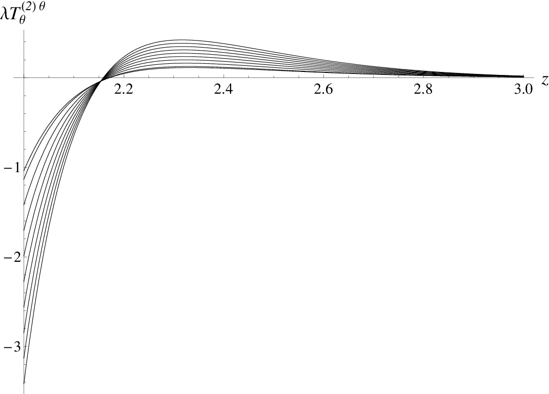
In Figs. 1-3 the run of the (rescaled) components of the stress-energy tensor as functions of for a few exemplary values of the coupling parameter from the range is displayed. Although there are strong dependence on some general features are common for all the curves. Indeed, the is negative at the event horizon and remains so for and attains a (positive) maximum. Subsequently it decreases with approaches a (negative) minimum and falls to zero. Inspection of Fig. 2 shows that is negative at the event horizon, approaches a (positive) maximum and fall to zero as Finally, the run of the angular component (Fig. 3) is qualitatively similar to that of The behavior of the stress-energy for more exotic values of the coupling parameter can easily be inferred form the general formulas (10-12). Specifically, at the event horizon one has
| (13) |
and
| (14) |
Thus far we have carried out our calculations using the Planck units. It is of some interest to restore the constants and in the final expressions describing the renormalized stress-energy tensor. Simple manipulations give
| (15) |
where and are dimensionless functions of
Since the Schwinger-DeWitt approximation is local and the geometry at the event horizon is regular, one expects that the stress-energy tensor is also regular there. On the other hand, the stress-energy tensor is regular in the physical sense if it is regular in a coordinate system which is well behaved as For example, the components of the stress-energy tensor in a freely falling frame, denoted here as , and are
| (16) |
| (17) |
| (18) |
where is the energy per unit mass along the geodesic and Inspection of Eqs. (16-18) shows that if all components of and are finite on the horizon the stress-energy tensor in a freely falling frame is finite as well.
Now, simple calculations show that the difference between radial and time components of the stress-energy factors
| (19) |
where
| (20) |
| (21) |
and, consequently, both tensors are regular in a physical sense. Moreover, using our general formula describing the stress- energy tensor it can be shown that it remains so in any static and spherically-symmetric spacetime.
III The back reaction problem
Having constructed the next-to-leading term of the renormalized stress-energy tensor which depends on a general metric one can analyze the back reaction of the quantized field upon the black hole geometry. It should be emphasized once more that accepting the approximation (5) we ignore particle creation which is a nonlocal effect. To simplify our discussion we shall assume that the cosmological constant and the renormalized coupling parameters and in the quadratic part of the total action
| (22) |
where is the Weyl tensor, identically vanish. The semiclassical Einstein field equations have, therefore, a standard form
| (23) |
where is the renormalized stress-energy tensor.
Since the total stress-energy tensor depends functionally on a wide class of metrics, one can, in principle, construct the self-consistent solution of the system (23). It should be noted however, that since the general stress-energy tensor, is constructed from it contains the terms up to eight derivatives of and, consequently, there is a real danger that the semiclassical equations may lead to physically unacceptable solutions [25]. Moreover, the tensor is extremely complicated and it is natural that one is forced to refer to some approximations. Here we shall treat the right hand side of the semiclassical Einstein field equations as perturbation. Restricting to the perturbative solutions of the effective theory may be, therefore, the only one way to obtain the (approximate) physical solutions.
For the quantized massless fields in the Schwarzschild geometry the back reaction program has been initiated by York [26]. Subsequently, it has been applied in numerous papers [27, 28, 29, 30, 31], where various aspects of the back reaction of the massive fields upon the black hole geometry has been studied using the first order approximation to the stress-energy tensor.
In the semiclassical approach we ignore the effects caused by the quantized gravitational field simply because they are not known. On general grounds, however, it is expected that the perturbations of the classical metrics caused by gravitons should be of the same order as from the other quantized fields. One can justify neglecting of the graviton contribution to the total stress-energy tensor taking a large number of various fields in the calculations. It can be argued that the contribution of the gravitons would be small as compared with the total effect caused by other physical fields.
Now, let us introduce the dimensionless parameter [32] and make the substitution Expanding the metric tensor as
| (24) |
inserting it into the semiclassical equations (23) and collecting the terms with the like powers of the auxiliary parameter, one obtains
| (25) |
and
| (26) |
i.e., the modifications of the geometry caused by stress-energy tensor calculated in the corrected black hole spacetime, are ignored as these additional terms would be In other words we are looking for corrections to the classical solution.
From Eqs. (7-12) one sees that the solution of the back reaction problem reduces to elementary quadratures. First, let us consider the issue of the integration constants which appear in solutions of the differential equations. The zeroth-order equations will yield two integration constants, say, and which can be set to and respectively. Here is a “bare” mass of the black hole and can be determined from the condition On the other hand, the integration constant appearing in the component of the metric tensor can be absorbed in a process of the finite renormalization of mass. Indeed, it can be demonstrated that with the substitution
| (27) |
the radial component of the metric tensor can be written as
| (28) |
where and are given respectively by
| (29) |
and
| (30) |
Similarly, for to one has
| (31) |
where
| (32) |
The integration constant can be fixed by demanding that the time component of the metric tensor approaches its Minkowskian value as that is equivalent to normalizing the time coordinate at infinity.
As before, it is of some interest to restore the physical constants. Putting and in Eq.(28) the radial component of the metric tensor can schematically be written as
| (33) |
where and are simple polynomials depending parametrically on and their exact form can easily be inferred from Eq. (33). A similar expression can be constructed for and the result can be schematically written in the form
| (34) |
where comprise another pair of simple polynomials.
The location of the event horizon of the quantum-corrected Schwarzschild black hole is determined by the equation Putting one concludes that is given by
| (35) |
The Euclidean version of the line element (6) obtained with the aid of the Wick rotation has no conical singularity provided the “time” coordinate is periodic with a period given by
| (36) |
For the quantum-corrected metric (28-32), the period is
| (37) |
to the first order in
The surface gravity, which is proportional to the temperature of the black hole can be calculated (for the Lorentzian metric) from a simple relation
| (38) | |||||
where is a timelike Killing vector. The Hawking temperature, is, therefore, given by
| (39) | |||||
It should be noted that the temperature, when expressed in terms of the total mass of the system as seen by a distant observer, is independent of the coupling constant.
On the other hand, one can express the results (28-32) in terms of the horizon defined mass, which, of course, differs from the total mass of the system as seen by a distant observer. It can be achieved, for example, by inverting Eq. (35) and the elementary manipulations give
| (40) |
Consequently, one can systematically substitute Eq. (40) in Eqs.(28-32), expand and finally linearize the thus obtained results.
Equally well, one can start with a slightly different representation of the line element putting
| (41) |
expanding the functions and into the power series
| (42) |
| (43) |
and retaining only the linear terms. Now, accepting the boundary condition repeating the calculations for the line element (41), with the integration constants appearing in the solution for determined either from and or from and one can easily reconstruct all our previous results.
IV final remarks
In this paper we report our calculations of the next-to-leading term of the renormalized stress-energy tensor of the quantized massive scalar field in a large mass limit. To achieve this, we have calculated the effective action constructed form the (integrated) coincidence limit of the coefficients and and, subsequently, we have calculated the approximate stress-energy tensor by functional differentiation of the thus obtained action with respect to the metric tensor. The obtained stress-energy tensor can be employed in any spacetime provided the condition holds. The general formulas describing the stress-energy tensor are extremely complex, but, when applied to the Schwarzschild geometry, they yield remarkably simple result, which is the main result of this paper. The general stress-energy tensor has been used in the analysis of the back reaction of the quantized field upon the geometry of the Schwarzschild black hole.
Finally, we indicate a few possible directions of investigations. First, it would be interesting to examine the vacuum polarization effects in more complex backgrounds, as for example, the spacetime of the electrically charged black holes with or without the cosmological constant. Further, the numeric approach to the back reaction would certainly strengthen our understanding of the problem. This group of problems is actively investigated and the results will be published elsewhere.
References
- [1] A. O. Barvinsky and G. A. Vilkovisky, Phys. Rept. 119, 1 (1985).
- [2] V. P. Frolov and A. I. Zelnikov, Phys. Rev. D29, 1057 (1984).
- [3] B. S. DeWitt, Dynamical Theory of groups and fields (Gordon and Breach, New York, 1965).
- [4] T. Sakai, Tôhoku Math. J. 23, 589 (1971).
- [5] P. B. Gilkey, J. Differential Geometry 10, 601 (1975).
- [6] I. G. Avramidi, Theor. Math. Phys. 79, 494 (1989).
- [7] P. Amsterdamski, A. L. Berkin, and D. J. O’Connor, Class. Quant. Grav. 6, 1981 (1989).
- [8] A. E. M. van de Ven, Class. Quant. Grav. 15, 2311 (1998).
- [9] L. Parker, in Recent Developments In Gravitation (Cargese, 1978) (Academic Press, New York, 1979).
- [10] M. Brown, Class. Quant. Grav. 2, 535 (1985).
- [11] J. A. M. Vermaseren (2000), eprint math-ph/0010025.
- [12] M. Tentyukov and J. A. M. Vermaseren (2007), eprint hep-ph/0702279.
- [13] J. Matyjasek, Phys. Rev. D 61, 124019 (2000).
- [14] J. Matyjasek, Phys. Rev. D 63, 084004 (2001).
- [15] V. P. Frolov and A. I. Zel’nikov, Phys. Lett. B 115, 372 (1982).
- [16] V. P. Frolov and A. I. Zel’nikov, Phys. Lett. B 123, 197 (1983).
- [17] P. R. Anderson, W. A. Hiscock, and D. A. Samuel, Phys. Rev. D 51, 4337 (1995).
- [18] A. A. Popov, Phys. Rev. D67, 044021 (2003).
- [19] B. E. Taylor, W. A. Hiscock, and P. R. Anderson, Phys. Rev. D61, 084021 (2000).
- [20] W. Berej and J. Matyjasek, Phys. Rev. D66, 024022 (2002).
- [21] J. Matyjasek, Phys. Rev. D74, 104030 (2006).
- [22] J. Matyjasek, Phys. Rev. D76, 084003 (2007).
- [23] W. A. Hiscock, S. L. Larson, and P. R. Anderson, Phys. Rev. D56, 3571 (1997).
- [24] B. E. Taylor, W. A. Hiscock, and P. R. Anderson, Phys. Rev. D55, 6116 (1997).
- [25] L. Parker and J. Z. Simon, Phys. Rev. D47, 1339 (1993).
- [26] J. W. York, Phys. Rev. D31, 775 (1985).
- [27] C. O. Lousto and N. G. Sanchez, Phys. Lett. B212, 411 (1988).
- [28] D. Hochberg, T. W. Kephart, and J. W. York, Phys. Rev. D48, 479 (1993).
- [29] D. Hochberg and T. W. Kephart, Phys. Rev. D47, 1465 (1993).
- [30] D. Hochberg, T. W. Kephart, and J. W. York, Phys. Rev. D49, 5257 (1994).
- [31] P. R. Anderson, W. A. Hiscock, J. Whitesell, and J. W. York, Phys. Rev. D50, 6427 (1994).
- [32] C. M. Bender and S. A. Orszag, Advanced mathematical methods for scientists and engineers. (Springer-Verlag, New York, 1999).