Proposed lower bound for the shear viscosity to entropy density ratio in some dense liquids
Abstract
Starting from relativistic quantum field theories, Kovtun et al. (2005) have quite recently proposed a lower bound , where is the shear viscosity and the volume density of entropy for dense liquids. If their proposal can eventually be proved, then this would provide key theoretical underpinning to earlier semiempirical proposals on the relation between a transport coefficient and a thermodynamic quantity . Here, we examine largely experimental data on some dense liquids, the insulators nitrogen, water, and ammonia, plus the alkali metals, where the shear viscosity for the four heaviest alkalis is known to scale onto an ‘almost universal’ curve, following the work of Tankeshwar and March a decade ago. So far, all known results for both insulating and metallic dense liquids correctly exceed the lower bound prediction of Kovtun et al.
Keywords:
Thermodynamic and transport properties; Liquids; Alkali metals.1 Background and outline
Going back, at very least, to the early semiempirical proposal of Rosenfeld [1], quite an active field has grown up relating shear viscosity to the volume density of entropy in dense liquids [2, 3, 4]. Some motivation for returning to this general area, however, has come from unexpected quarters, namely relativistic quantum field string theory methods. Thus, Kovtun et al. [5], starting from such an ab initio viewpoint, have proposed that the ratio has a lower bound given by Ks. Here, and denote Planck’s and Boltzmann’s constants, respectively. While the lower bound proposal is not yet proven, their arguments are highly plausible (see Section 5 for a brief summary).
The outline of the present paper is then as follows. After a brief review of the hard sphere model in Section 2, with specific emphasis to its results for the shear viscosity and entropy density in dense fluids, in Section 3, we examine some scaling properties of the three dense insulating liquids He, N2, and H2O considered in [5], as well as NH3. This is then followed in Section 4 by work on dense liquid metals [6]. Some six liquid transition metals treated computationally by means of the embedded atom model are then considered, with the alkalis playing the dominant role because of already known scaling properties of the transport coefficient for the four heaviest alkali metals, Na through Cs [7], these results constituting Section 4.2. A discussion follows in Section 5, together with proposals for further work that should prove fruitful.
2 Hard sphere model of shear viscosity and entropy density in a dense fluid used in phenomenological context
We begin with what we believe is the simplest model of a dense fluid, viz. that composed of hard spheres (HS). In early work, Collins and Raffel [8] and Longuet-Higgins and Pople [9] stressed that in a liquid of rigid molecules the singular nature of the interaction allows a finite flux of momentum and energy even when the liquid radial distribution function is momentarily isotropic, as it is in equilibrium.
The results obtained by Longuet-Higgins and Pople [9] can be displayed in terms of the deviation of the equation of state from the ideal gas form as
| (1) |
where denotes the hard sphere diameter, while is the particle mass. The factor in square brackets in Eq. (1) embodies the probability of finding two spheres at contact, which in turn is given by the contact value of the pair distribution function .
The Percus-Yevick theory [10, 11, 12] of the hard sphere fluid leads to a number of analytic, though of course approximate, results, which will be used below in exemplifying the hard sphere dense fluid predictions pertaining to the Kovtun et al. [5] lower bound on the ratio shear viscosity to volume density of entropy .
The so-called excess entropy and other thermodynamic properties of the density hard sphere fluid can be usually derived with adequate accuracy from the Carnahan-Starling [13] equation of state. In terms of the packing fraction , this reads
| (2) |
where , with being the number density. Eq. (2) can be generalized to embrace hard fluids of non-spherical molecules as [14]
| (3) |
with for tetrahedral molecules, and for spherical molecules, in which case it reduces to Eq. (2). Hence, by specifying the pressure as in the examples considered by Kovtun et al. [5], number density and temperature are related via the packing fraction by Eq. (2). Insertion of Eq. (2) in the right-hand side of Eq. (1) then yields .
To construct the Kovtun ratio in this model, we next write the excess entropy in the form
| (4) |
where is the entropy for an ideal gas [15],
| (5) |
the latter functional form, including an additive constant, being derived through thermodynamic considerations only e.g. by March and Tosi [16].
The excess entropy in Eq. (4) is clearly positive in the range . Dense fluids, for orientation, freeze when . The volume density of entropy for the dense hard sphere fluid is hence known from Eq. (4). The ratio can then be formed from Eqs. (1) and (4), and plotted as a function of , after eliminating through the hard sphere equation of state Eq. (2) choosing the pressure MPa [5] (Fig. 1). Appendix A gives a formal proof relating to under isobaric conditions, that is a function of , as in Fig. 1 (see also Fig. 2).

3 Shape similarity after scaling of available experimental data on dense insulating liquids helium, nitrogen, water, and ammonia
Though our main focus will be on dense metallic liquids, it seemed natural to start by examining scaling properties for helium, nitrogen, and water, the insulating liquids already considered by Kovtun et al. [5] along with their pioneering proposal. In their Fig. 2, all three liquids are treated in their plot of the ratio vs absolute temperature .
Because of the lower bound proposal, we have replotted their data in Fig. 2a. This scales with , and also scales in units of the value at the minimum, . It is of interest that for these very different liquids, the data collapses somewhat to exhibit considerable shape similarity. For completeness, as well as to gain insight as to the source of the minima in Fig. 2a, we show and separately in Fig. 2b for nitrogen, water, and ammonia. Over the range of temperatures displayed there, the viscosity is featureless, and it is the entropy density that has the characteristic features. It is noteworthy that the maximum in for water is near to the critical temperature . This is also true for nitrogen.


Having examined these four dense insulating liquids, we turn to our central examples, an embedded atom model computer simulation of six liquid transition metals, and, following that, the dense metallic alkali liquids Li through Cs.

4 Some relevant results concerning transport in liquid metals
So far, the specific dense liquids for which we have presented experimental results are insulators: atomic He and molecular fluids H2O and N2. Though we do not have such complete experimental data, we feel it of interest to summarize here some obviously relevant results on some twelve or so liquids having itinerant electrons, viz. liquid transition metals (Cu, …) and the five liquid alkali metals Li, Na, K, Rb, and Cs.
4.1 Computer simulation results on some liquid transition metals
Hoyt et al. [3] have carried out important computer simulation results of liquid transition metals, using as interatomic potential for their studies those generated by the embedded atom model (EAM). The transport coefficient they focussed on was the self diffusion . They were able to refine, for Cu, Ag, Au, Ni, Pd, and Pt, the earlier important study of Dzugotov [2], who approximated the excess entropy via the pair distribution function . Hoyt et al. [3] found a form like that of the semiempirical proposal of Rosenfeld [17], who wrote (see also Ref. [16])
| (6) |
where , with the excess entropy. Hoyt et al. [3] recovered a form like Eq. (6) for the six transition metals listed above, but with the factor to good accuracy. The scatter of Dzugotov’s results [2] was substantially reduced by the computer simulation results of Hoyt et al. [3].
As suitable results for excess entropy are not available to us, we next note two points: (i) The Stokes-Einstein relation (see Ref. [16]) can be used to estimate the viscosity of the above transition metals from the Hoyt et al. form for , and (ii) it is of obvious interest to examine the relation of the above to the predictions of the hard sphere model discussed above. This is because of the early study of Bernasconi and March [18] (see also Ref. [19]). These authors calculated from experiment near freezing the direct correlation function at , which for hard spheres the Percus-Yevick theory invoked above predicted to be related to its Fourier transform, say , by [20]
| (7) |
Table 1 shows the values obtained by Bernasconi and March [18] for four of the six liquid transition metals considered in the EAM studies of Hoyt et al. [3].
| Metal | |||
|---|---|---|---|
| Cu | 60 | 47 | 1.3 |
| Ag | 51 | 53 | 1.0 |
| Au | 35 | 38 | 0.9 |
| Ni | 41 | 50 | 0.8 |
A necessary condition for a liquid metal to be ‘hard-sphere’-like is for the ratio to be near unity, as stressed by Bernasconi and March [18]. This is well satisfied for Ag, Au, and Ni (Tab. 1). The polyvalent liquid metals Ga, Pb, and Sb are obvious exceptions from the study of Bernasconi and March [18], the ratios being respectively 0.2, 0.4, and 0.3.
Because of the results in Table 1, we have been motivated to return to the hard sphere model. However, we have transcended the analytic model of Longuet-Higgins and Pople [9] used above, by invoking computer simulation results. Thus, Speedy [21] has fitted molecular dynamics results for in the hard sphere model by the approximate formula
| (8) |
where is proportional to the packing fraction introduced above, while
| (9) |
is the infinite dilution value of , which is known exactly from kinetic theory.
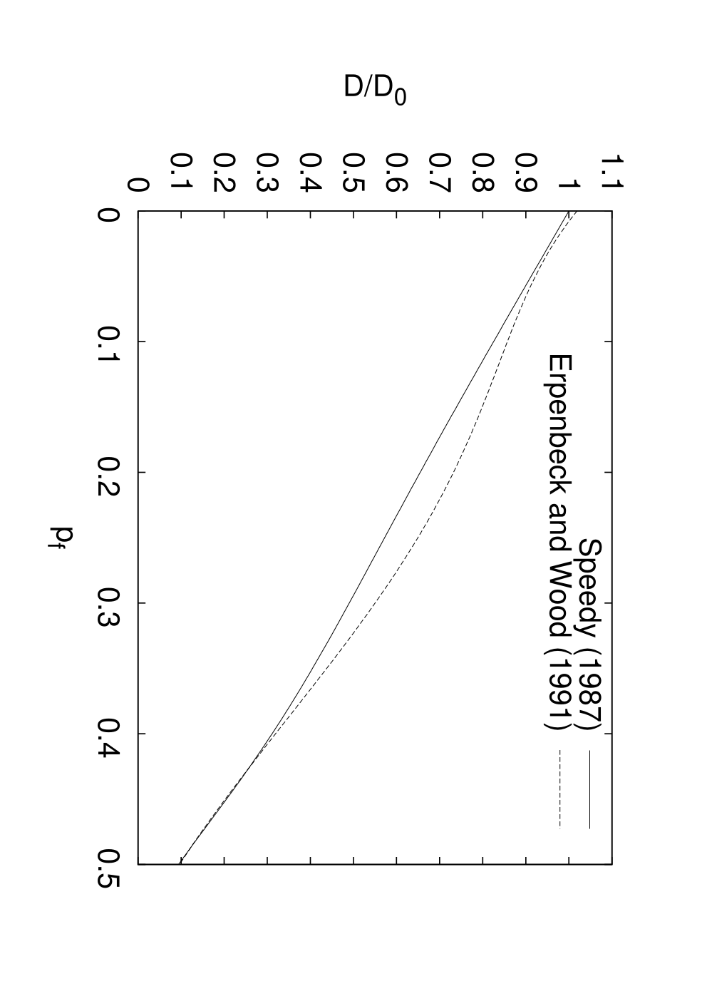
For comparison with Eq. (8) due to Speedy [21], an alternative expression for the density dependence of the self-diffusion for hard spheres has been given by Erpenbeck and Wood [22] as
| (10) |
where
| (11) |
denoting the hard sphere pair distribution function at contact, referred to earlier in relation to the Longuet-Higgins and Pople [9] study. This is related to the packing fraction by
| (12) |
Eqs. (8) and (10) are then compared in Fig. 4 as a function of packing fraction . Since our main focus here is the shear viscosity , we have used the, of course approximate, proposal of Longuet-Higgins and Pople [9] for the specific form of the Stokes-Einstein relation, viz.
| (13) |
to plot vs in Fig. 5.

4.2 Scaled experimental data on liquid alkali metals
To conclude this section, it seemed of interest to refer to scaling properties of the five liquid alkali metals Li, Na, K, Rb, and Cs [7]. Why the liquid alkali metals are especially important in the present context is clear from the scaling exhibited in [7] of the shear viscosity from available experiments. In fact the so-called fluidity is the quantity plotted, but appropriately scaled by its value at the melting temperature , to distinguish from the minimum in the plot of the ratio vs (Fig. 2).

We have redrawn Fig. 3 of Ref. [7] in Fig. 6 and it is quite clear that, for the four heavier alkalis, Na, K, Rb, and Cs, the scaling used collapses the data onto an ‘almost universal’ curve. While there is some shape similarity for the remaining (lightest) alkali metal Li, this has an appreciably different magnitude, under scaling, from the other four. In principle, one can estimate the volume density of entropy as a function of from experimental structure factor data.


In fact, in a further paper [17], Rosenfeld writes an empirical formula relating shear viscosity and scaled entropy , where
| (14) |
referring to the ideal gas as in Eq. (3). Writing [17]
| (15) |
where is the particle number density, while is the ionic mass, Rosenfeld proposes the semiempirical formula
| (16) |
Hence, it follows [17] that
| (17) |
We have employed the experimental viscosity data in Ref. [24] for liquid Li (see also Fig. 6), to extract the Rosenfeld scaled excess entropy from Eq. (17), when combined with the approximate equation of state of Chapman and March [23]. This reads
| (18) |
where is the coupling parameter of the so-called one component plasma (see [25]) defined by
| (19) |
where . Fig. 7b shows schematic plots of vs , which it would, of course, be of considerable interest to have quantitative experimental results in the future at the thermodynamic conditions in Fig. 6 and in the experimental study of in Ban et al. [24]. Fig. 7c finally shows the schematic form of the volume density of entropy obtained from Eqs. (6) and (5).
5 Discussion and future directions
Motivated by the proposal of Kovtun et al. [5] of a lower bound for the ratio of shear viscosity to volume density of entropy , we have studied this ratio for some fifteen dense liquids. These include liquid metals, five liquid alkalis, plus some six liquid transition metals, for the former of which the shear viscosity has been determined experimentally over a range of temperature . Using the scaling of these data in [7], Figure 6 has been constructed by making use of the semiempirical Eq. (16) given by Rosenfeld [1, 17]. Into this equation, the experimental data for has first been used to predict the volume density of entropy plotted in Fig. 7. It will be of significance for the future to refine these data using X-ray or neutron diffraction measurements to estimate semiempirically the pair correlation function . This is then sufficient to determine the entropy , following, for instance, the procedure of Dzugotov [2].
The most quantitative results in the present study are presented in Fig. 2. In part (a), we have scaled data for the four insulating liquids shown by plotting the ratio vs , where is the temperature at the minimum of in each case. It is seen that there is considerable shape similarity for the four liquids, in spite of the range of isobaric conditions involved. Fig. 2b is presented, again from experiment, to give insight into the origin of the minima in . Over the range plotted in Fig. 2b, is monotonically decreasing with increasing temperature, and the minimum in therefore arises from the turning point in the volume density of entropy , at temperature . Fig. 2c shows that both and are of the order of the critical temperature for N2, H2O, and NH3.
The remainder of the article begins a study of the ten liquid metals already mentioned. Because of the incomplete availability of (i) experiment and (ii) computer simulation data, we have had recourse to models. These are (i) the well known HS model, set out in Section 2, where both approximate analytic theory and computer simulation data is now available (see especially Fig. 4 for the diffusion coefficient ). This has been combined with the (of course approximate) analytic form of the Stokes-Einstein Eq. (13) to construct Fig. 5. It would, of course, be valuable to have results for the shear viscosity paralleling those displayed in Fig. 4 for , to test the HS predictions of Fig. 5, and if necessary to refine them.
We may mention also at this point the generalization Eq. (3) of the HS equation of state (2). It has been suggested [14] that Eq. (3) may have some relevance to water with , which is close to the numerical value 1.7 employed to construct Fig. 3, relating to experiments on water and ammonia. While on the HS model, the ‘softening’ of the core to inverse power repulsive potentials is referred in Appendix B (see also especially Fig. 8).
For the ten or so liquid metals considered, and beginning with the six transition elements studied by Hoyt et al. [3] using the embedded atom model, Table 1 shows that a necessary, though not sufficient, condition for HS behavior (that the final column is equal to unity) is well obeyed for two, Ag and Au, and is approximately valid for Cu and Ni. So in the future, it will be interesting to bring computer simulation and experiment into contact with the HS model, and especially with the predictions for the shear viscosity in Fig. 5. Finally, for the five liquid alkalis, Fig. 6 summarizes scaling properties of the shear viscosity. However, experimental results on the density-temperature relation under the thermodynamic conditions appropriate to Fig. 6 and to the isotope experiments of Ban et al. [24] would be most helpful in the present context, as, next to of course He (see Fig. 2), Li is the most likely candidate for quantal effects, and thus for a possible lower bound to compare with the prediction of Kovtun et al. [5].
In a related vein, we note that the work of Tosi [26] on electron plasma theory has led to the conclusion that the itinerant electrons in the alkali metals contribute less than 10% to the shear viscosity. As a proposal for future work, though somewhat esoteric, it would be of interest to study in its own right the homogeneous electron liquid [27].
As for liquid Li, we believe it would be of considerable interest to use a density-dependent pair potential, such as that derived by Parrot and March [28] from first principles electron theory, to calculate the excess entropy approximately from the resulting pair distribution function , as set out in [2]. Then, adding the ideal entropy in Eq. (5), one could plot the volume density of entropy, say, along an isobar. This could then be compared for any shape similarity with the three insulating liquids treated in Fig. 2b.
As this study was nearing completion, we became aware of the highly relevant work of Schäfer [29]. This author studied the ratio for trapped fermions in the unitarity limit. The result of this investigation was the prediction that is roughly in units of . This example prompts us to conclude this article by summarizing briefly the uncertainty principle argument pointed out by Kovtun et al. [5]. This consists of three parts: (i) for a plasma is proportional to , where is the energy density while is the typical mean free time of a quasiparticle, and (ii) the entropy density is proportional to the density of quasiparticles, say , i.e. . Thus the desired ratio . The third part of the argument [5] invokes, as mentioned above, the uncertainty principle in the form , without which the concept of quasiparticle lacks meaning. This gives , without, however, the factor in [5].
Acknowledgements
NHM began his contribution to this study at the Abdus Salam International Centre for Theoretical Physics. It is a pleasure to thank Professor V. E. Kravtsov for generous hospitality. The work of NHM was brought to fruition during a stay at the University of Catania. NHM was partially supported by the University of Antwerp through the BOF-NOI.
Appendix A Scaled diffusion coefficient in terms of excess entropy in the hard sphere model: Relation to the work of Kovtun et al.
In Fig. 4 we compare the computer simulation results of Speedy [21] with those of Erpenbeck and Wood [22]. Evidently, with refinements to available computer data, the two curves in Fig. 4 will converge to a single curve which we represent by writing the scaled diffusion coefficient in the functional form
| (20) |
But for this HS model, we know the excess entropy in the Percus-Yevick approximation as is given in Eq. (4). From Fig. 4 representing an approximation to the formally exact Eq. (20), we can conclude that a unique inversion exists, to yield
| (21) |
Inserting Eq. (21) into Eq. (4), we therefore conclude that there exists the functional relation
| (22) |
in the HS model.
If we combine this exact formal result, Eq. (22) with the (now approximate) Stokes-Einstein relation proposed by Longuet-Higgins and Pople [9] for the HS model, Eq. (13), and use to find
| (23) |
we find from Eqs. (20) and (23) that
| (24) |
But with the plausible assumption that Eq. (22) has the unique inversion
| (25) |
we find by combining this equation with Eq. (24) that
| (26) |
We propose that Eq. (26) demonstrates the functional form of in terms of the dimensionless excess entropy in the HS model.
But when we turn to consider the ratio as in the lower bound proposed by Kovtun et al. [5], we note that the total entropy is given by Eq. (14). While in Eq. (22) is solely a function of the packing factor , involves also, following Landau and Lifshitz [15], the thermal de Broglie wavelength , providing a natural length unit for the volume per particle , and hence the volume entropy depends on , , and , as does the free energy since the ideal gas result reads [15]
| (27) |
In the isobaric plots of Fig. 2, , and one has that .
Appendix B Results for inverse power repulsive potentials
In the main text, together with experiments and their interpretation especially on the molecular insulating liquids nitrogen, water, and ammonia, we have given prominence to the hard sphere model. Here, we generalize this model to the case of inverse power repulsive potentials having the form
| (28) |
The merit of this model is that, for any such inverse power potential, thermodynamic properties are readily accessible since only a single isotherm, isochoric, or isobar needs to be known. Then all other properties can be found, as discussed by Hoover and Ross [30].
Quite specifically, for pair-wise additive potentials having the form (28), (now dimensionless) thermodynamic properties depend only on the one density-demperature variable, say:
| (29) |
where is proportional to the packing fraction and is defined as .
We have studied the data on nitrogen and water presented in Sec. 3 of the main text, and for we find remarkable shape similarity (Fig. 8).

Because of transport coefficients being another focal point here, we finish this Appendix by referring to the interesting study of the diffusion coefficient for the potential (28) by Heyes and Powles [31]. For a packing fraction of 0.044, these authors studied how approached the hard sphere limit and found that their data could be well fitted by the form, with now in dimensionless form,
| (30) |
indicating a rather slow approach to the hard sphere result.
References
- [1] Y. Rosenfeld, Phys. Rev. A 15, 2545 (1977).
- [2] M. Dzugotov, Nature 381, 137 (1996).
- [3] J. J. Hoyt, M. Asta, and B. Sadigh, Phys. Rev. Lett. 85, 594 (2000).
- [4] C. Kaur, U. Harbola, and S. P. Das, J. Chem. Phys. 123, 034501 (2005).
- [5] P. K. Kovtun, D. T. Son, and A. O. Starinets, Phys. Rev. Lett. 94, 111601 (2005).
- [6] N. H. March, Liquid metals. Concepts and theory (Cambridge University Press, Cambridge, 1990).
- [7] K. Tankeshwar and N. H. March, Phys. Chem. Liq. 37, 39 (1998).
- [8] F. C. Collins and H. Raffel, J. Chem. Phys. 22, 1728 (1954).
- [9] H. C. Longuet-Higgins and J. A. Pople, J. Chem. Phys. 25, 884 (1956).
- [10] J. K. Percus and G. J. Yevick, Phys. Rev. 110, 1 (1958).
- [11] E. Thiele, J. Chem. Phys. 39, 474 (1963).
- [12] M. S. Wertheim, Phys. Rev. Lett. 10, 321 (1963).
- [13] N. F. Carnahan and K. F. Starling, J. Chem. Phys. 51, 635 (1969).
- [14] J. J. Kolafa and I. Nezbeda, Mol. Phys. 84, 421 (1995).
- [15] L. D. Landau and E. M. Lifshitz, Statistical Physics (Pergamon, Oxford, 1980).
- [16] N. H. March and M. P. Tosi, Introduction to Liquid State Physics (World Scientific, Singapore, 2002).
- [17] Y. Rosenfeld, J. Phys.: Condens. Matter 11, 5415 (1999).
- [18] J. M. Bernasconi and N. H. March, Phys. Chem. Liq. 15, 169 (1986).
- [19] N. H. March, J. Chem. Phys. 76, 1869 (1982).
- [20] A. B. Bhatia and N. H. March, J. Chem. Phys. 80, 2076 (1984).
- [21] R. J. Speedy, Mod. Phys. 62, 509 (1987).
- [22] J. J. Erpenbeck and W. W. Wood, Phys. Rev. A 43, 4254 (1991).
- [23] R. G. Chapman and N. H. March, Phys. Chem. Liq. 16, 77 (1986).
- [24] N. T. Ban, C. M. Randall, and D. J. Montgomery, Phys. Rev. 128, 6 (1962).
- [25] N. H. March and M. P. Tosi, Coulomb liquids (Academic, New York, 1984).
- [26] M. P. Tosi, Nuovo Cimento D 14, 559 (1992).
- [27] G. Giuliani and G. Vignale, Quantum Theory of the Electron Liquid (Cambridge University Press, Cambridge, 2005).
- [28] F. Perrot and N. H. March, Phys. Rev. A 42, 4884 (1990).
- [29] T. Schäfer, Phys. Rev. A 76, 063618 (2007).
- [30] W. G. Hoover and M. Ross, Contemp. Phys. 12, 339 (1971).
- [31] D. M. Heyes and J. G. Powles, Mol. Phys. 95, 259 (1998).