The trapped region

Let $(M,g,K)$ be a Cauchy hypersurface in a 3+1 dimensional Lorentzian spacetime $\mathcal{M}$. Let $\Sigma$ be a spacelike surface in $M$ with null normals $\ell^{\pm}$, see figure 1.

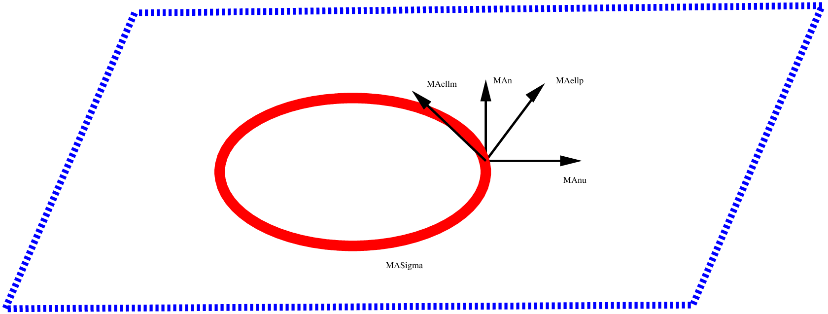
We set

Then $A$ is the second fundamental form of $\Sigma$ in $M$, $K^{\Sigma}$ is the restriction of $K$ to $\Sigma$, and $\chi^{\pm}$ are the null second fundamental forms associated to $\ell^{\pm}$. Taking traces yields

Then $H$ is the mean curvature of $\Sigma$ in $M$, $P$ is the trace of $K^{\Sigma}$ on $\Sigma$ and $\theta^{\pm}$ are the null expansions of $\Sigma$. We declare $\ell^{+}$ to be the outer null normal.

Recall that $\theta^{+}$ is the logarithmic variation of area along $\ell^{+}$,

If $\Sigma$ is a MOTS then outgoing null rays are marginally collapsing. We call $\Sigma$ (weakly) outer trapped if ($\theta^{+}\leq 0$) $\theta^{+}<0$. The null energy condition (NEC) holds if $G(v,v)\geq 0$ for any null vector $v$, where $G=\operatorname{Ric}-\frac{1}{2}\operatorname{Sc}g$ is the Einstein tensor.

The usual definition of trapped surface is $\theta^{+}<0$, $\theta^{-}<0$. By the singularity theorems of Hawking and Penrose, a maximal globally hyperbolic spacetime satisfying suitable energy conditions, eg., NEC, and which contains a trapped surface, is causally incomplete. We note that also the presence of an outer trapped surface implies incompletness. In particular, if NEC holds in $\mathcal{M}$ and $\mathcal{M}$ contains a Cauchy surface $M$ with an outer trapped surface which separates and has noncompact exterior, then $\mathcal{M}$ is null geodesically incomplete, cf. (Gannon, 1976; Andersson et al., 2008). Thus MOTSs may be viewed as black hole boundaries.

The null expansion $\theta^{+}=P+H$ is elliptic when viewed as a functional of $\Sigma\subset M$, since, as is well known, the mean curvature $H$ has this property, and $P$ may be viewed as a lower order term. For variations along $\ell^{+}$, we have

so $|\Sigma|$ is not an elliptic functional with respect to null variations. However, variations within $M$, of the form $\delta_{f\nu}\theta^{+}$ define an elliptic operator, see section 1.2 below.

It is well known that if there are surfaces $\Sigma_{\pm}$ with $H[\Sigma_{+}]>0$ and $H[\Sigma_{-}]<0$, which form barriers for the problem of minimizing area, then there is a minimal ($H=0$) surface between them. Suppose we have an analogue for MOTSs of existence in the presence of barriers, in this case surfaces $\Sigma_{\pm}$ with the inner barrier satisfying $\theta^{+}[\Sigma_{-}]<0$, while the outer barrier satisfies $\theta^{+}[\Sigma_{+}]>0$. Then, in view of (1), MOTSs should persist if NEC holds. This can in fact be proved using the results of (Andersson and Metzger, 2007), given an outer barrier, cf. (Andersson et al., 2008), see section 2.2. In particular, if $(M,g,K)$ is an asymptotically flat initial data set, then there is an outer barrier in $M$. We shall, throughout the rest of this note, assume the presence of an outer barrier.

Due to the persistence of MOTSs, we expect that MOTSs are generically in a marginally outer trapped tube (MOTT), i.e. a hypersurface of $\mathcal{M}$, foliated by MOTSs. This has been proved for outermost MOTSs, modulo a genericity condition, cf. theorem 1 and (Andersson et al., 2008). In this case, the MOTT is weakly spacelike if NEC holds. If in addition $\theta^{-}<0$ on the MOTS, the MOTT is a dynamical horizon, cf. (Ashtekar and Krishnan, 2002; Ashtekar and Galloway, 2005).

Let $Lf=\delta_{f\nu}\theta^{+}$. Then

where $S(X)=K(X,\nu)$. The operator $L$ is the analogue of the minimal surface stability operator. We note the following facts which hold for $L$. The operator $L$ is 2:nd order elliptic and non-self adjoint in general. There is a unique principal eigenvalue $\lambda\in\mathbb{R}$, with positive eigenfunction $\phi$. If $\Sigma$ is a locally outermost MOTS then $\lambda\geq 0$. Further, if $\lambda\geq 0$ then there is $f\geq 0$ such that $Lf\geq 0$, i.e., if $\lambda\geq 0$ the maximum principle holds.

In particular, if $\Sigma$ is locally outermost then $\Sigma$ is stable.

The proof of the following theorem makes use of the definition of $L$, the implicit function theorem, as well as the above mentioned version of the maximum principle. The following theorem was proved in (Andersson et al., 2005; Andersson et al., 2008).

Theorem 1 is a local result. In general, the outermost MOTS can jump. This may happen for example through the formation of a new MOTS outside the existing ones, a process that can be caused by the coalescence of black holes, cf. section 3.1. As a MOTS is created, the MOTT bifurcates in general, see (Andersson et al., 2008), see also figure 2.

The proof of theorem 2 applies several techniques used in (Schoen et al., 1975), including the Simons identity, a Kato inequality, and the Hoffmann-Spruck Sobolev inequality. The Moser iteration used in (Schoen et al., 1975) to achieve the $L^{\infty}$ estimate for $|A|$ is replaced by a Stampacchia iteration. Further, the symmetrized stability estimate of (Galloway and Schoen, 2006) is used. By applying the local area bound of Pogorelov, it is possible to avoid a dependence on the area $|\Sigma|$ in the curvature estimate. Due to the use of this result, which in turn relies upon the Gauss-Bonnet theorem, the above form of the curvature estimate applies only to the case of a 2-dimensional surface in a 3+1 dimensional spacetime.

Consider $\mathbb{R}\times M$, with metric $ds^{2}+g$, see figure 3. Define $\overline{K}$ by pullback of $K$. Let $\overline{M}$ be the graph of $f$.

On $\overline{M}$ we have induced mean curvature $\mathcal{H}$ and $\mathcal{P}=\operatorname{tr}_{\overline{M}}\overline{K}$. Jang’s equation is

This is the analogue of the equation $\theta^{+}=0$

By translation invariance, $J[f]=J[f+t]$, we have that the stability operator for $\overline{M}$ has $L\phi=0$, with $\phi=\langle\nu,e_{4}\rangle$. Here $L$ is the analogue of the minimal surface stability operator for $\overline{M}$. By the work in (Schoen and Yau, 1981), we have local curvature bounds for $\overline{M}$, which yields compactness. This allows one to prove existence of solutions to Jang’s equation using a capillarity deformation together with Leray-Schauder theory. One considers the deformed equation

As $\sigma$ goes from 0 to 1, we have a limit $f_{\tau}$. Letting $\tau\searrow 0$, we have by compactness, convergence of a subsequence of $f_{\tau}$ to a solution $f$ of Jang’s equation. The solution has blowups in general. As observed in (Schoen and Yau, 1981), blowups project to MOTSs, cf. figure 4.

Therefore Jang’s equation can be used to prove existence of MOTSs. It was proved in (Andersson and Metzger, 2007) that the blowup surfaces are stable MOTSs.

Theorem 3 provides the analogue of the barrier argument for existence of minimal surfaces. The proof considers a sequence of Dirichlet problems for Jang’s equation, which forces a blowup solution. We solve

see figure 5. If we let $Z\to\infty$, then the solution converges to solution with blowups.

In order to prove boundary gradient estimates necessary to apply Leray-Schauder theory, one makes use of a deformation of the Cauchy surface, see figure 6, to get $H>0$ at $\partial M$. The limiting solution must blow up somewhere, which implies the existence of a MOTS. We have a foliation by barriers near $\partial M$. Using this fact, and the maximum principle, one can show the MOTSs constructed are in the undeformed region of $M$.

By deforming the data inside $\partial^{-}M$, we can allow $\theta^{+}[\partial^{-}M]\leq 0$. We remark that (Eichmair, 2007) has studied the Plateau problem for MOTSs using Perron’s method.

By Rauchaudhuri, $\delta_{\ell^{+}}\theta^{+}=-W\leq 0$ if NEC holds.

Based on theorem 4, it seems natural to view the collection of outermost MOTS in $M_{t}$ as the black hole boundary in $\mathcal{M}$. If it is smooth, this collection is a MOTT. For further regularity and continuation results for MOTTs, cf. (Andersson et al., 2008).

It is a direct consequence of the gluing and heat flow construction used in the proof of the area bound, that if $\Sigma_{1},\Sigma_{2}$ are locally outermost MOTSs which are sufficiently close, then there is a MOTS $\Sigma$ surrounding them. This may be interpreted as stating that black holes must coalesce once they are sufficiently close. The phenomenon described here is seen in numerical simulations. As the MOTS $\Sigma$ is formed in an evolution, it has principal eigenvalue $\lambda=0$ and generically there is a MOTT which bifurcates into existence when $\Sigma$ is formed. See (Andersson et al., 2008) for details.

I thank the Mittag-Leffler-Institute, Djursholm, Sweden for hospitality and support. This work was supported in part by the NSF, under contract no. DMS 0407732 and DMS 0707306 with the University of Miami.

References

- Gannon (1976) D. Gannon, General Relativity and Gravitation 7, 219–232 (1976).
- Andersson et al. (2008) L. Andersson, M. Mars, J. Metzger, and W. Simon (2008), 0811.4721.
- Andersson and Metzger (2007) L. Andersson, and J. Metzger (2007), 0708.4252.
- Ashtekar and Krishnan (2002) A. Ashtekar, and B. Krishnan, Phys. Rev. Lett. 89, 261101, 4 (2002).
- Ashtekar and Galloway (2005) A. Ashtekar, and G. J. Galloway, Adv. Theor. Math. Phys. 9, 1–30 (2005).
- Andersson et al. (2005) L. Andersson, M. Mars, and W. Simon, Phys. Rev. Lett. 95, 111102 (2005), gr-qc/0506013.
- Andersson and Metzger (2005) L. Andersson, and J. Metzger (2005), gr-qc/0512106.
- Schoen et al. (1975) R. Schoen, L. Simon, and S. T. Yau, Acta Math. 134, 275–288 (1975).
- Galloway and Schoen (2006) G. J. Galloway, and R. Schoen, Comm. Math. Phys. 266, 571–576 (2006).
- Schoen and Yau (1981) R. Schoen, and S. T. Yau, Comm. Math. Phys. 79, 231–260 (1981).
- Schoen (2004) R. Schoen (2004).
- Eichmair (2007) M. Eichmair, The Plateau problem for apparent horizons (2007), arXiv.org:0711.4139.
- Galloway (2008) G. J. Galloway, Comm. Anal. Geom. 16, 217–229 (2008).
- Eichmair (2008) M. Eichmair, Existence, regularity, and properties of generalized apparent horizons (2008), arXiv.org:0805.4454.
- Schoen and Yau (1983) R. Schoen, and S. T. Yau, Comm. Math. Phys. 90, 575–579 (1983).
- Yau (2001) S. T. Yau, Adv. Theor. Math. Phys. 5, 755–767 (2001).
- Galloway and O’Murchadha (2008) G. J. Galloway, and N. O’Murchadha, Class. Quant. Grav. 25, 105009 (2008), 0802.3247.