Stochastic resonance in bistable confining potentials

The simplest dynamical system displaying stochastic resonance (SR) is a Brownian particle bound into a one-dimensional double well under the action of a time oscillating tilt and subjected to fluctuating forces (noise) [1, 2]. The SR mechanism can be revealed as a maximum in the amplitude of the periodic component of the average particle position as a function of the noise intensity (temperature). Due to fluctuations, the particle randomly jumps between the two potential wells with Kramers rate [3] that depends on the double well potential and temperature. When the average escape time of the particle out of the potential minima (i.e., the inverse of the Kramers rate) approximately equals the half time-period of the applied perturbation, the noise induced interwell jumps and the periodic force synchronize, thus leading to SR.

When studying the problem of a Brownian particle in a symmetric double well periodically tilted in time, the corresponding potential $U(x)$ is usually assumed to diverge like $U(x)\sim x^{4}$ at large $x$ [1, 3], so as to ensure a robust confining action. However, the divergence of the potential for $|x|\to\infty$ strongly affects the response of the system to an external time-periodic forcing. The goal of the present paper is to investigate how the Brownian motion in a double well changes with the confining strength of the one-dimensional potential $U(x)$. For simplicity we assume that $U(x)\sim|x|^{q}$ for $x\to\pm\infty$. By studying the dependence of a SR spectral quantifier on $q$, we conclude that bistability is a necessary, but not sufficient condition for a one-dimensional system to exhibit SR.

The model discussed in the following represents an overdamped Brownian particle with coordinate $x$. Its dynamics is described by the Langevin equation,

where $(\dots)^{\prime}\equiv\mathrm{d}(\dots)/\mathrm{d}x$. The confining potential,

is obtained by superimposing a Gaussian repulsive barrier of height $U_{0}$ and width $L_{0}$, to a power-law potential well. To ensure confinement, our analysis is restricted to $q>1$. The total potential is mirror symmetric at $x=0$, i.e. $U(x)=U(-x)$. Depending on $q$ a potential $U(x)$ is called hard (super-harmonic) for $q>2$, or soft (sub-harmonic) for $q<2$ [4]. The periodic drive $A(t)$ is chosen as

with amplitude, $A_{0}$, angular frequency, $\Omega\equiv 2\pi\nu$, and time origin arbitrarily set to zero. The fluctuating force $\xi(t)$ is modeled as a stationary zero-mean Gaussian noise with auto-correlation function $\langle\xi(t)\xi(t^{\prime})\rangle=2\eta k_{\mathrm{B}}T\delta(t-t^{\prime})$. Here $T$ is the temperature and $\eta$ the friction coefficient.

For numerical purposes it is convenient to choose $U_{0}$, $L_{0}$, and $\tau\equiv\eta L_{0}^{2}/U_{0}$ as the new units respectively of energy, space and time. Correspondingly, the variables and the parameters appearing in Eq. (1) can be replaced by the dimensionless quantities $\tilde{x}=x/L_{0}$, $\tilde{t}=t/\tau$, $\tilde{k}=L_{0}^{q}k/U_{0}$, $\tilde{A}_{0}=A_{0}L_{0}/U_{0}$, $\tilde{\Omega}=\Omega\tau$, and $\tilde{T}=k_{B}T/U_{0}$. To avoid a cumbersome notation, in the following we omit all the tildes. In dimensionless notation the potential (2) reads,

and the Langevin equation (1) can be rewritten as

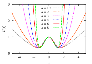
after the Gaussian noise $\xi(t)$ has been further rescaled so that $\langle\xi({t})\rangle=0$ and $\langle\xi({t})\xi({t}^{\prime})\rangle=2\delta({t}-{t}^{\prime})$. In the following we study how changing $q$ influences the response of the particle to the periodic forcing signal $A(t)$. As a result of rescaling, the height, $U_{0}$, and the width, $L_{0}$, of the potential barrier, as well as the friction coefficient, $\eta$, have been set to one. The remaining tunable parameter $k$ of the potential (4) will be kept fixed to $k=0.2$ throughout the present paper. Due to the Gaussian nature of the potential barrier, the barrier height, $\Delta U$, and the potential minima, $\pm x_{m}$, weakly depend on $q$ (see Fig. 1); therefore, the observed residual SR dependence on $q$ is mostly an effect of the varying confining strength of the potential.

We have simulated the behavior of the system by numerically integrating the rescaled Langevin equation (5) through a Milshtein algorithm [5, 6]. Stochastic trajectories were simulated for different time lengths $t_{\mathrm{max}}$ and time steps $\Delta t$, so as to ensure appropriate numerical accuracy and transient effects subtraction. Average quantities have been obtained as ensemble averages over at least $10^{4}$ trajectories.

In the long time regime, after transient effects subsided, the response $\langle x(t)\rangle$ of a particle moving in a symmetric bistable potential $U(x)$ under the action of the signal (3) with small-amplitude, $A_{0}x_{m}\ll\Delta U$, and low-frequency, $\Omega\ll U^{\prime\prime}(x_{m})$, results from the interplay of inter- and the intrawell dynamics [1]. On ignoring for the time being the intrawell dynamics, the system response at low temperatures is dominated by its harmonic component [1, 7, 8, 9, 10]

with amplitude, $\bar{x}(T)$, and phase, $\bar{\phi}(T)$, approximated by

Here $r\propto\exp(-\Delta U/T)$ is the Kramers rate and $\langle x^{2}\rangle_{0}$ the variance of the stationary unperturbed process $x(t)$ ($A_{0}=0$), both temperature dependent quantities. The amplitude $\bar{x}(T)$ can be manipulated by tuning the noise level. Note that Eqs. (6)-(8) hold in the linear response theory limit, only, i.e., for $A_{0}x_{m}\ll T$ and $\Omega>r$ [11, 12].

According to Eq. (7), in the limit $T\to 0$ the amplitude $\bar{x}(T)$ vanishes due to the potential barrier. The rate $r$ for the particle to overcome the potential barrier decreases to zero exponentially when lowering the temperature, that is $r\ll\Omega$. The interwell jumps are thus inhibited and the particle gets locked in either minima with probability $1/2$; hence $\lim_{T\to 0}\langle{x}\rangle=0$. In contrast, for high temperatures, $T\gg\Delta U$, $r$ may grow much larger than $\Omega$ and, consequently, $\bar{x}(T)\simeq\langle x^{2}\rangle_{0}/T$. For a hard potential with $q>2$ we show below that $\langle x^{2}\rangle_{0}\sim T^{2/q}$, so that, again, $\lim_{T\to\infty}\bar{x}(T)=0$. The occurrence of these limits for $T\to 0$ and $T\to\infty$ implies the existence of a maximum of $\bar{x}(T)$ for some optimal $T\sim\Delta U$. This is the so-called spectral characterization of SR [1].

We conclude this note with two important remarks:

(i) The coexistence of two locally stable minima separated by a potential barrier is commonly advocated to explain the occurrence of a SR peak in a continuous bistable dynamics. Here we have shown that this keeps being true as long as the confining action exerted by the potential is super-harmonic. Most notably, for harmonic and sub-harmonic potentials the periodic component of the system response may increase monotonically with the noise level.

(ii) In many experimental reports (see, for a review, Ref. [16]), the authors tried to characterize the SR peak by means of Eq. (6), without paying much attention to the $T$ dependence of the quantity $\langle x^{2}\rangle_{0}$. In some cases they adopted an outright two-state model with $\langle x^{2}\rangle_{0}=x_{m}^{2}$. This led to a poor fit of the decaying tail of $\bar{x}(T)$, whereas a more accurate fit could have given a valuable clue to better model the system at hand [17].

This work has been supported by the Estonian Science Foundation through Grant No. 7466 (M.P., E.H.), Spanish MEC and FEDER through project FISICOS (FIS2007-60327), and ESF STOCHDYN project (E.H.).

References

- (1) L. Gammaitoni, P. Hänggi, P. Jung, and F. Marchesoni, Rev. Mod. Phys. 70, (1998) 223.
- (2) R. Benzi, A. Sutera, and A. Vulpiani, J. Phys. A 14, (1981) L453.
- (3) P. Hänggi, P. Talkner, and M. Borkovec, Rev. Mod. Phys. 62, (1990) 251.
- (4) F. Marchesoni, P. Sodano, and M. Zannetti, Phys. Rev. Lett. 61, (1988) 1143.
- (5) P. Kloeden and E. Platen, Numerical Solution of Stochastic Differential Equations (Springer, Berlin, 1999).
- (6) G. Milsten and M. Tretyakov, Stochastic Numerics for Mathematical Physics (Springer, Berlin, 2004).
- (7) B. McNamara and K. Wiesenfeld, Phys. Rev. A 39, (1989) 4854.
- (8) C. Presilla, F. Marchesoni, and L. Gammaitoni, Phys. Rev. A 40, (1989) 2105.
- (9) Gang Hu, H. Haken, and C. Z. Ning, Phys. Lett. A 172 (1992) 21.
- (10) P. Jung and P. Hänggi, Phys. Rev. A 44, (1991) 8032.
- (11) P. Jung and P. Hänggi, Z. Phys. B 90, (1993) 255; J. Casado-Pascual, J. Gomez-Ordonez, M. Morillo, and P. Hänggi, Europhys. Lett. 58, (2002) 342.
- (12) V. A. Shneidman, P. Jung, and P. Hänggi, Phys. Rev. Lett. 72, (1994) 2682.
- (13) L. Gammaitoni, F. Marchesoni, E. Menichella-Saetta, and S. Santucci, Phys. Rev. E 51, (1995) R3799.
- (14) A. R. Bulsara, K. Lindenberg, and K. E. Shuler, J. Stat. Phys. 27, (1982) 787.
- (15) J. J. Collins, C. C. Chow, and T. T. Imhoff, Nature 376, (1995) 236.
- (16) A. Bulsara, P. Hänggi, F. Marchesoni, F. Moss, and M. Shlesinger, Proceedings of the NATO ARW on Stochastic Resonance in Physics and Biology, J. Stat. Phys. 70, (1993) 1.
- (17) L. Gammaitoni, F. Marchesoni, M. Martinelli, L. Pardi, and S. Santucci, Phys. Lett. A 158, (1991) 449.