Higher order analogues of the Tracy-Widom distribution and the Painlevé II hierarchy

T. Claeys A. Its I. Krasovsky

Abstract

We study Fredholm determinants related to a family of kernels which describe the edge eigenvalue behavior in unitary random matrix models with critical edge points. The kernels are natural higher order analogues of the Airy kernel and are built out of functions associated with the Painlevé I hierarchy. The Fredholm determinants related to those kernels are higher order generalizations of the Tracy-Widom distribution. We give an explicit expression for the determinants in terms of a distinguished smooth solution to the Painlevé II hierarchy. In addition we compute large gap asymptotics for the Fredholm determinants.

1 Introduction

In unitary random matrix ensembles with a probability measure of the form

\frac{1}{Z_{n}}e^{-n\,{\rm tr\,}V(M)}dM,

(1.1)

on the Hermitian $n\times n$ matrices, where $V$ is real analytic on $\mathbb{R}$ with sufficient growth at infinity, various correlation functions of eigenvalues can be expressed in terms of the kernel

K_{n}(x,y)=\frac{e^{-\frac{n}{2}V(x)}e^{-\frac{n}{2}V(y)}}{x-y}\frac{\kappa_{n-1}}{\kappa_{n}}(p_{n}(x)p_{n-1}(y)-p_{n}(y)p_{n-1}(x)),

(1.2)

constructed from the polynomials

p_{k}(x)=\kappa_{k}x^{k}+\cdots,\qquad\qquad\mbox{$\kappa_{k}>0$,}

orthonormal with respect to the weight $e^{-nV}$ on $\mathbb{R}$ .

The limiting mean eigenvalue density is known, see e.g. [15], to be given as the density of an equilibrium measure $\mu_{V}$ minimizing the logarithmic energy

I_{V}(\mu)=\iint\log\frac{1}{|x-y|}d\mu(x)d\mu(y)+\int V(x)d\mu(x),

(1.3)

among all probability measures $\mu$ on $\mathbb{R}$ . The equilibrium density depends on the potential $V$ but can in general be written in the form [19]

\psi_{V}(x)=\frac{d\mu_{V}(x)}{dx}=\frac{1}{\pi}\sqrt{Q_{V}^{-}(x)},\qquad Q_{V}^{-}(x)=\begin{cases}-Q_{V}(x),&\mbox{if }Q_{V}(x)<0,\cr 0,&\mbox{otherwise},\end{cases}

where $Q_{V}$ is a real analytic function determined by $V$ . Generically $Q_{V}$ has simple zeros at the endpoints of ${\operatorname{supp}}\,\psi_{V}$ , so that $\psi_{V}$ vanishes as a square root [36]. For special (non-regular or critical) $V$ ’s however, the limiting mean eigenvalue density vanishes faster. In general, $Q_{V}$ has a zero of order $4k+1$ , $k=0,1,\dots$ at an endpoint of the support.

Remark 1.1

$Q_{V}$ cannot have zeros of order $4k+3$ . These endpoint behaviors would contradict variational conditions that follow from the minimization property of the equilibrium measure [20].

Example 1.2

The simplest non-regular case $k=1$ is realized, e.g., for a critical quartic potential

V(x)=\frac{1}{20}x^{4}-\frac{4}{15}x^{3}+\frac{1}{5}x^{2}+\frac{8}{5}x.

(1.4)

Here the limiting mean eigenvalue density is supported on $[-2,2]$ and given by

\psi_{V}(x)=\frac{1}{10\pi}(x+2)^{1/2}(2-x)^{5/2}\chi_{[-2,2]}(x).

(1.5)

It is easy to verify (1.4) by substituting this $\psi_{V}(x)$ into the variational conditions. In fact, it is much easier to recover $V$ starting from a given limiting mean eigenvalue density than to find the limiting mean eigenvalue density corresponding to a given potential $V$ directly.

In order to construct polynomial potentials $V$ for which $k\geq 1$ , it is necessary that the degree of $V$ is at least $2k+2$ .

In the generic case where $k=0$ for the rightmost endpoint $b=b_{V}$ of ${\operatorname{supp}}\,\psi_{V}$ , it follows from the results of Deift et al [20, 16] that, for any fixed $u$ and $v$ ,

\lim_{n\to\infty}\frac{1}{cn^{2/3}}K_{n}(b+\frac{u}{cn^{2/3}},b+\frac{v}{cn^{2/3}})=K^{(0)}(u,v),

(1.6)

where

K^{(0)}(u,v)=\frac{{\rm Ai\,}(u){\rm Ai\,}^{\prime}(v)-{\rm Ai\,}(v){\rm Ai\,}^{\prime}(u)}{u-v}

(1.7)

is the Airy kernel, and $c=c_{V}$ is a constant depending on $V$ . Let $\lambda_{n}$ be the largest eigenvalue of a random matrix $M$ . It was proved in many cases [39, 16] and is believed to hold for $k=0$ in general that the limiting distribution of $\lambda_{n}$ is given by

\lim_{n\to\infty}{\rm Prob}\left(cn^{2/3}(\lambda_{n}-b)<s\right)=\det(I-K_{s}^{(0)}),

(1.8)

where $K_{s}^{(0)}$ is the Airy-kernel trace-class operator acting on $L^{2}(s,\infty)$ .

The function at the r.h.s. of (1.8) is known as the Tracy-Widom distribution. Tracy and Widom [39] discovered a representation

\det(I-K_{s}^{(0)})=\exp\left(-\int_{s}^{+\infty}(y-s)q_{0}^{2}(y)dy\right)

(1.9)

in terms of the Hastings-McLeod solution $q_{0}$ of the Painlevé II equation

q_{xx}=xq+2q^{3}

(1.10)

characterized by the asymptotic behavior

		$\displaystyle q_{0}(x)\sim{\rm Ai\,}(x),$	as $x\to+\infty$ ,		(1.11)
		$\displaystyle q_{0}(x)=\sqrt{\frac{-x}{2}}\left(1+\frac{1}{8x^{3}}+O\left(x^{-6}\right)\right),$	as $x\to-\infty$ .		(1.12)

The Tracy-Widom function $\det(I-K_{s}^{(0)})$ does not only describe the largest eigenvalue distribution in random matrix ensembles, but appears also in several combinatorial models, for example, it provides the distribution of the longest increasing subsequence of random permutations [3].

In the general case of arbitrary $k$ , a family of limiting kernels $K^{(k)}(u,v)$ appears in place of the Airy kernel. Consider a potential $V(x)$ such that $Q_{V}(x)$ has a zero of order $4k+1$ , $k=0,1,\dots$ at the rightmost endpoint of ${\operatorname{supp}}\,\psi_{V}$ . Furthermore, to obtain more general results, consider for suitable $V_{j}(x)$ the deformation

\widetilde{V}(x)=V(x)+\sum_{j=0}^{2k-1}T_{j}V_{j}(x),

where $T_{j}$ are constants. The natural analogues of (1.6) are double-scaling limits where $n\to\infty$ and simultaneously $T_{j}\to 0$ at an appropriate rate in $n$ characterized by parameters $t_{j}$ (in the simplest case we can take all $T_{j}=t_{j}=0$ ). We refer to [12] for more details about those double-scaling limits in the case $k=1$ . In these limits we expect the following expressions for the kernel (corresponding to $\widetilde{V}(x)$ ) and the distribution of the largest eigenvalue, according to conjectures in the physics literature [6, 8]:

\lim_{n\to\infty}\frac{1}{cn^{2/(4k+3)}}K_{n}(b+\frac{u}{cn^{2/(4k+3)}},b+\frac{v}{cn^{2/(4k+3)}})=K^{(k)}(u,v;t_{0},\dots,t_{2k-1}),

(1.13)

for certain constants $b$ and $c$ and any fixed $u$ , $v$ . Here

K^{(k)}(u,v;t_{0},\ldots,t_{2k-1})=\frac{\Phi_{1}^{(2k)}(u)\Phi_{2}^{(2k)}(v)-\Phi_{1}^{(2k)}(v)\Phi_{2}^{(2k)}(u)}{-2\pi i(u-v)},

(1.14)

where the functions $\Phi_{j}^{(2k)}(w)=\Phi_{j}^{(2k)}(w;t_{0},\ldots,t_{2k-1})$ are described below. Moreover,

\lim_{n\to\infty}{\rm Prob}\left(cn^{2/(4k+3)}(\lambda_{n}-b)<s\right)\\ =\lim_{n\to\infty}\det(I-K_{n}\chi_{(b+s/[cn^{2/(4k+3)}],+\infty)})=\det(I-K_{s}^{(k)}),

(1.15)

where $K_{n}\chi_{(a,b)}$ is the operator with kernel $K_{n}$ acting on $L^{2}(a,b)$ , and $K_{s}^{(k)}$ is the trace-class operator with kernel (1.14) acting on $L^{2}(s,\infty)$ .

Note that (1.13) for the case $k=1$ was proved in [12]. Our goal in this paper is not to prove (1.13) and (1.15). Rather, we study the properties of $\det(I-K_{s}^{(k)})$ .

The functions $\Phi_{1}^{(2k)}=\Phi_{1}^{(2k)}(\zeta;t_{0},\ldots,t_{2k-1})$ and $\Phi_{2}^{(2k)}=\Phi_{2}^{(2k)}(\zeta;t_{0},\ldots,t_{2k-1})$ appear as solutions of the Lax pair associated with a distinguished solution to the $2k$ -th member of the Painlevé I hierarchy [6, 8, 12]. They are most easily characterized in terms of the following Riemann-Hilbert (RH) problem.

RH problem for $\Phi$

Figure 1: Contour for the

\Phi

-RH problem.

(a)

$\Phi=\Phi^{(2k)}:\mathbb{C}\setminus\Gamma\to\mathbb{C}^{2\times 2}$ is analytic, with

\Gamma=\cup_{j=1}^{4}\Gamma_{j}\cup\{0\},\qquad\Gamma_{1}=\mathbb{R}^{+},\quad\Gamma_{3}=\mathbb{R}^{-},\quad\Gamma_{2}=e^{\frac{-i\pi}{4k+3}}\mathbb{R}^{-},\quad\Gamma_{4}=e^{\frac{i\pi}{4k+3}}\mathbb{R}^{-},

oriented as in Figure 1.

(b)

$\Phi$ has $L^{2}$ boundary values $\Phi_{+}$ as $\zeta$ approaches $\Gamma$ from the left (w.r.t. the direction shown by an arrow), and $\Phi_{-}$ , from the right. They are related by the jump conditions

$\displaystyle\Phi_{+}(\zeta)=\Phi_{-}(\zeta)\begin{pmatrix}0&1\\ -1&0\end{pmatrix},$	for $\zeta\in\Gamma_{3}$ ,	(1.16)
$\displaystyle\Phi_{+}(\zeta)=\Phi_{-}(\zeta)\begin{pmatrix}1&1\\ 0&1\end{pmatrix},$	for $\zeta\in\Gamma_{1}$ ,	(1.17)
$\displaystyle\Phi_{+}(\zeta)=\Phi_{-}(\zeta)\begin{pmatrix}1&0\\ 1&1\end{pmatrix},$	for $\zeta\in\Gamma_{2}\cup\Gamma_{4}$ .	(1.18)

(c)

$\Phi$ has the following behavior as $\zeta\to\infty$ :

\Phi(\zeta)=\zeta^{-\frac{1}{4}\sigma_{3}}N\left(I+\Phi_{\infty}\zeta^{-1/2}+{\cal O}(\zeta^{-1})\right)e^{-\theta(\zeta)\sigma_{3}},

(1.19)

where $\Phi_{\infty}$ is independent of $\zeta$ (its explicit expression will not be important below), $\sigma_{3}$ is the Pauli matrix $\begin{pmatrix}1&0\\ 0&-1\end{pmatrix}$ , $N$ is given by

N=\frac{1}{\sqrt{2}}\begin{pmatrix}1&1\\ -1&1\end{pmatrix}e^{-\frac{1}{4}\pi i\sigma_{3}},

(1.20)

and

\theta(\zeta;t_{0},\ldots,t_{2k-1})=\frac{2}{4k+3}\zeta^{\frac{4k+3}{2}}-2\sum_{j=0}^{2k-1}\frac{(-1)^{j}t_{j}}{2j+1}\zeta^{\frac{2j+1}{2}},

(1.21)

where the fractional powers denote (as usual throughout this paper) the principal branches analytic for $\zeta\in\mathbb{C}\setminus(-\infty,0]$ and positive for $\zeta>0$ .

(d)

$\Phi$ is bounded near $0$ .

The functions $\Phi_{1}=\Phi_{1}^{(2k)}$ and $\Phi_{2}=\Phi_{2}^{(2k)}$ appearing in (1.14) are the analytic extensions of the functions $\Phi_{11}$ and $\Phi_{21}$ from the sector in between $\Gamma_{1}$ and $\Gamma_{2}$ to the entire complex plane. (One verifies the analyticity by multiplying the jump matrices: see Remark 2.2.)

A solution $\Phi$ to this RH problem satisfies a linear system of the form

\Phi_{\zeta}^{\prime}=A\Phi,\qquad\Phi_{t_{j}}^{\prime}=B_{j}\Phi,

(1.22)

where $A$ is a polynomial in $\zeta$ of degree $2k+1$ , and $B_{j}$ is a polynomial in $\zeta$ of degree $j+1$ . The compatibility conditions for the system (1.22) yield the ${\rm P}_{\rm I}^{(2k)}$ equation, the Painlevé I equation of order $4k$ . The most general form of the RH problem for ${\rm P}_{\rm I}^{(2k)}$ involves a contour consisting of $4k+4$ rays instead of $4$ . Our RH problem is the one corresponding to one particular solution of ${\rm P}_{\rm I}^{(2k)}$ , which was introduced by Brézin, Marinari, and Parisi in [8]. The precise structure of the Painlevé I hierarchy and the relation of the functions $\Phi_{1}$ and $\Phi_{2}$ to the ${\rm P}_{\rm I}^{(2k)}$ equation is not important for us, but we refer the interested reader to [35, 32, 33]. The Fredholm determinant $\det(I-K_{s}^{(k)})$ is the object we want to study, and we only need to know the RH characterization of $\Phi_{1}$ and $\Phi_{2}$ for that purpose.

Remark 1.3

In the case $k=1$ , the existence of a RH solution $\Phi$ was proved in [11, Lemma 2.3] for all real values of $t_{0},t_{1}$ . The proof of this fact is however valid for arbitrary $k$ and arbitrary real values of the parameters $t_{j}$ . It is important to stress that the proof does not hold for odd members of the Painlevé I hierarchy, in other words for the function $\Phi^{(2k+1)}$ . Moreover, the RH problem for $\Phi^{(1)}$ is not solvable for every real $t_{0}$ , because this would imply [21, 11] the existence of a real-valued Painlevé I solution without poles on the real line, which contradicts [29]. However, as a consequence of Remark 1.1, only the kernels generated by the even members of the Painlevé I hierarchy appear in unitary random matrix ensembles of the form (1.1).

Remark 1.4

It should be noted that the RH problem for $\Phi^{(2k)}$ is not uniquely solvable: there is a family of solutions of the form $\begin{pmatrix}1&0\\ \omega&1\end{pmatrix}\Phi^{(2k)}(\zeta)$ , where $\omega$ can depend on $t_{0},\ldots,t_{2k-1}$ but not on $\zeta$ . Indeed it is obvious that the left multiplication by a constant matrix (independent of $\zeta$ ) does not modify the jump conditions. If the matrix is lower-triangular with $1$ on both diagonal entries, neither the asymptotic condition (1.19) is violated. One verifies as in [28] that, up to the left multiplication by such a matrix, the RH problem is uniquely solvable. However, the kernel (1.14) is independent of the choice of a solution and thus is well-defined.

It follows from (1.14) and (1.19) that

K^{(k)}(u,v;t_{0},\ldots,t_{2k-1})={\cal O}(e^{-cu^{\frac{4k+3}{2}}-cv^{\frac{4k+3}{2}}}),\qquad\mbox{ as $u,v\to+\infty$},

(1.23)

for some constant $c>0$ . Consequently, the asymptotics of $\ln\det(I-K_{s}^{(k)})$ can be obtained by a standard series expansion. In particular,

\ln\det(I-K_{s}^{(k)})={\cal O}(e^{-cs^{\frac{4k+3}{2}}}),\qquad\mbox{ as $s\to+\infty$}.

(1.24)

The question of the asymptotic behavior of $\det(I-K_{s}^{(k)})$ as $s\to-\infty$ is much more subtle and will be addressed below.

1.1 Statement of results

In the present paper, we will answer the following questions. What are the “large gap” asymptotics for the Fredholm determinant $\det(I-K_{s}^{(k)})$ as $s\to-\infty$ ? Can we find an identity for $\det(I-K_{s}^{(k)})$ which generalizes the Tracy-Widom formula (1.9) to general $k$ ? What is the analogue of the Hastings-McLeod solution of Painlevé II for general $k$ , and what are its properties?

1.1.1 Large gap asymptotics

The first goal of this paper is to find large gap asymptotics for the Fredholm determinant $\det(I-K_{s}^{(k)})$ as $s\to-\infty$ . Those asymptotics are known for the Airy kernel, i.e. in the case $k=0$ , namely

\ln\det(I-K_{s}^{(0)})=-\frac{|s|^{3}}{12}-\frac{1}{8}\ln|s|+\chi+{\cal O}(|s|^{-3/2}),

(1.25)

where

\chi=\frac{1}{24}\ln 2+\zeta^{\prime}(-1),

(1.26)

and $\zeta(s)$ is the Riemann zeta-function. The first two terms at the r.h.s. of (1.25) follow easily from (1.9) and (1.12). The expansion of the derivative of (1.25) was obtained by Tracy and Widom who also conjectured the value (1.26) for the constant $\chi$ [39]. A full proof of (1.25), (1.26) was given recently in [17] and another proof followed shortly in [2].

We obtain

Theorem 1.5

Let $K^{(k)}$ be the kernel defined in (1.14) for arbitrary $k=0,1,2,\dots$ , depending on parameters $t_{0},\ldots,t_{2k-1}$ , and write $K_{s}^{(k)}$ for the trace-class operator with kernel $K^{(k)}$ acting on $L^{2}(s,+\infty)$ . The asymptotic expansion for the Fredholm determinant $\det(I-K_{s}^{(k)})$ as $s\to-\infty$ is given by the formula

\frac{d}{ds}\ln\det(I-K_{s}^{(k)})=\frac{1}{4}a_{0}^{2}(s)|s|^{4k+2}+\frac{3a_{1}(s)}{16a_{0}(s)|s|}+{\cal O}(|s|^{-\frac{4k+5}{2}}).

(1.27)

Here $a_{0}(s,t_{0},\ldots,t_{2k-1})$ and $a_{1}(s,t_{0},\ldots,t_{2k-1})$ are defined as follows:

a_{j}(s)={1\over\Gamma(j+\frac{3}{2})}\left(\frac{\Gamma(2k+\frac{3}{2})}{\Gamma(2k+2-j)}\right.\\ \left.+\sum_{m=2}^{2k+1-j}t_{2k+1-m}\frac{\Gamma(2k+\frac{3}{2}-m)}{\Gamma(2k+2-j-m)}|s|^{-m}\right),

(1.28)

where the sum vanishes if $j=2k$ , $j=2k+1$ , and $\Gamma(x)$ is Euler’s $\Gamma$ -function.

Remark 1.6

Expanding the right-hand side of (1.27) in negative powers of $|s|$ and integrating, one easily finds asymptotics for $\det(I-K_{s}^{(k)})$ itself except for the constant of integration $\chi^{(k)}$ . In particular, to the leading order

\ln\det(I-K_{s}^{(k)})=-\left(\frac{(4k+1)!}{2^{4k+1}(2k)!(2k+1)!}\right)^{2}\frac{|s|^{4k+3}}{4k+3}\left[1+o(1)\right],

(1.29)

which was conjectured in [7, 9]. The constant $\chi^{(k)}$ has a representation, as in the Airy case $k=0$ , in terms of a solution of a Painlevé equation and also in terms of a limit of multiple integrals (see Section 6). For $k=0$ , the relevant multiple integral can be reduced to an explicitly computable Selberg integral, which allowed the authors in [17] to obtain the simple expression (1.26).

Example 1.7

For $k=0$ , we have $a_{0}(s)=1$ and $a_{1}(s)=\frac{2}{3}$ , so that (1.27) takes the form

\frac{d}{ds}\ln\det(I-K_{s}^{(0)})=\frac{1}{4}|s|^{2}+\frac{1}{8|s|}+{\cal O}(|s|^{-\frac{5}{2}}).

Integrating this expression gives (1.25) without fixing the constant $\chi$ .

For $k=1$ ,

a_{0}(s;t_{0},t_{1})=\frac{5}{8}+t_{1}|s|^{-2}+2t_{0}|s|^{-3},\qquad a_{1}(s;t_{0},t_{1})=\frac{5}{4}+\frac{2}{3}t_{1}|s|^{-2}.

Theorem 1.5 then gives

\frac{d}{ds}\ln\det(I-K_{s}^{(1)})=\frac{5^{2}}{2^{8}}|s|^{6}+\frac{5}{16}t_{1}|s|^{4}+\frac{5}{8}t_{0}|s|^{3}+\frac{1}{4}t_{1}^{2}|s|^{2}+t_{0}t_{1}|s|+t_{0}^{2}+\frac{3}{8|s|}+{\cal O}(|s|^{-3}),

which integrates to

\ln\det(I-K_{s}^{(1)})=-\frac{5^{2}}{2^{8}\cdot 7}|s|^{7}-\frac{1}{16}t_{1}|s|^{5}-\frac{5}{32}t_{0}|s|^{4}-\frac{1}{12}t_{1}^{2}|s|^{3}-\frac{1}{2}t_{0}t_{1}|s|^{2}-t_{0}^{2}|s|\\ +\chi^{(1)}-\frac{3}{8}\ln|s|+{\cal O}(|s|^{-2}),

(1.30)

where $\chi^{(1)}$ is the constant of integration. In Section 6, we discuss 2 representations for this constant mentioned in Remark 1.6.

1.1.2 The Painlevé II hierarchy

On our way to the higher order analogues of the Tracy-Widom formula, let us first describe the Painlevé II hierarchy and in particular one distinguished solution to it, which is a natural higher order analogue of the Hastings-McLeod solution to the Painlevé II equation.

The $n$ -th member of the Painlevé II hierarchy, the ${\rm P}_{{\rm II}}^{(n)}$ equation, is the following differential equation of order $2n$ for $q=q(x;\tau_{1},\ldots,\tau_{n-1})$ [38, 14, 30, 35]:

\left(\frac{d}{dx}+2q\right)\mathcal{L}_{n}[q_{x}-q^{2}]+\sum_{\ell=1}^{n-1}\tau_{\ell}\left(\frac{d}{dx}+2q\right)\mathcal{L}_{\ell}[q_{x}-q^{2}]=xq-\alpha,\qquad n\geq 1,

(1.31)

where the operator $\mathcal{L}_{n}$ is defined by the Lenard recursion relation

\frac{d}{dx}\mathcal{L}_{j+1}f=\left(\frac{d^{3}}{dx^{3}}+4f\frac{d}{dx}+2f_{x}\right)\mathcal{L}_{j}f,\qquad\mathcal{L}_{0}f=\frac{1}{2},\qquad\mathcal{L}_{j}0=0,\quad j\geq 1.

(1.32)

In particular, the first members of the hierarchy (we write $q_{x}^{(j)}$ for the $j$ -th derivative of $q$ with respect to $x$ ) are given by the formulas:

$\displaystyle{\rm P}_{{\rm II}}^{(1)}:$	$\displaystyle q_{xx}-2q^{3}=xq-\alpha,$	(1.33)
$\displaystyle{\rm P}_{{\rm II}}^{(2)}:$	$\displaystyle(q_{x}^{(4)}-10qq_{x}^{2}-10q^{2}q_{xx}+6q^{5})+\tau_{1}(q_{xx}-2q^{3})=xq-\alpha,$	(1.34)
$\displaystyle{\rm P}_{{\rm II}}^{(3)}:$	$\displaystyle(q_{x}^{(6)}-14q^{2}q_{x}^{(4)}-56qq_{x}q_{x}^{(3)}-70(q_{x})^{2}q_{xx}-42q(q_{xx})^{2}$
$\displaystyle\qquad+70q^{4}q_{xx}+140q^{3}q_{x}^{2}-20q^{7})+\tau_{2}(q_{x}^{(4)}-10qq_{x}^{2}-10q^{2}q_{xx}+6q^{5})$
$\displaystyle\qquad\qquad\qquad\qquad\qquad\qquad\qquad\qquad+\tau_{1}(q_{xx}-2q^{3})=xq-\alpha.$		(1.35)

We are interested in the odd members of the above hierarchy, with the value of the parameter $\alpha=\frac{1}{2}$ . One distinguished solution of the ${\rm P}_{{\rm II}}^{(n)}$ equation attracts our attention. It has the following properties.

Theorem 1.8

Fix $\tau_{1},\ldots,\tau_{n-1}\in\mathbb{R}$ . For $n$ odd and $\alpha=\frac{1}{2}$ , there exists a real solution $q=q(x;\tau_{1},\ldots,\tau_{n-1})$ of the ${\rm P}_{{\rm II}}^{(n)}$ equation (1.31) which has no poles for the real values of $x$ , and the following asymptotic behavior as $x\to\pm\infty$ :

		$\displaystyle q(x)=\frac{1}{2x}+{\cal O}(x^{-\frac{4n+1}{2n}}),$	$\displaystyle\qquad\mbox{ as $x\to+\infty$},$		(1.36)
		$\displaystyle q(x)=\left(\frac{n!^{2}}{(2n)!}\|x\|\right)^{\frac{1}{2n}}+{\cal O}(\|x\|^{-1}),$	$\displaystyle\qquad\mbox{ as $x\to-\infty$}.$		(1.37)

Remark 1.9

For $n=1$ , (1.36) and (1.37) together fix the solution to be the Hastings-McLeod solution of Painlevé II [26]. Note that the function $q$ differs from the function $u$ given by (1.10)-(1.12), which is the Hastings-McLeod solution corresponding to the value $\alpha=0$ , while $q$ corresponds to $\alpha=\frac{1}{2}$ . We will explain below why the case $\alpha=\frac{1}{2}$ , and not $\alpha=0$ , is relevant for the Fredholm determinant if $k\geq 1$ . For general odd $n$ , although the ${\rm P}_{{\rm II}}^{(n)}$ equation is of order $2n$ , it is our belief that (1.36) and (1.37) together still (as for $n=1$ ) determine the real solution $q$ uniquely. We do not have a proof of this fact, but we will provide some supporting heuristic arguments later on.

Remark 1.10

The asymptotics (1.36) at $+\infty$ indicate that the terms at the right-hand side of (1.31) are dominant compared to those at the left-hand side, and that there is a balance between the terms $xq$ and $\alpha=\frac{1}{2}$ . There is a whole family of solutions sharing the local asymptotic behavior (1.36), see [30]. The asymptotics (1.37) at $-\infty$ indicate a balance of the $q^{2n+1}$ -term at the left-hand side with the term $xq$ at the right-hand side. Again the existence of solutions with this local behavior was shown in [30].

Remark 1.11

It is a well-known fact that there is a one-to-one map between the solutions of a Painlevé equation and a so-called monodromy surface [23]. The solution considered in Theorem 1.8 is mapped to the point on the monodromy surface corresponding to the Stokes multipliers

		$\displaystyle s_{2}=s_{3}=\cdots=s_{2n}=0,$
		$\displaystyle s_{1}=s_{2n+1}=-i.$

We will characterize this Painlevé transcendent in Section 5 in terms of a RH problem.

1.1.3 Painlevé expression for the Fredholm determinants

Let $n=2k+1$ . Define $b_{j}=b_{j}(s;t_{0},\ldots,t_{2k-1})$ for $j=0,\ldots,2k$ slightly modified compared to $a_{j}$ (1.28) by

b_{j}(s)=\frac{\Gamma(2k+\frac{3}{2})}{\Gamma(j+\frac{3}{2})\Gamma(2k+2-j)}s^{2k+1-j}\\ -\sum_{\ell=j}^{2k-1}(-1)^{\ell}t_{\ell}\frac{\Gamma(\ell+\frac{1}{2})}{\Gamma(j+\frac{3}{2})\Gamma(\ell-j+1)}s^{\ell-j},

(1.38)

and let $x=x(s;t_{0},\ldots,t_{2k-1})$ and $\tau_{j}=\tau_{j}(s;t_{0},\ldots,t_{2k-1})$ be polynomials in $s$ defined by

		$\displaystyle x(s)=-2^{\frac{4k+1}{4k+3}}b_{0}(s;t_{0},\ldots,t_{2k-1}),$			(1.39)
		$\displaystyle\tau_{j}(s)=(2j+1)2^{\frac{4(k-j)+1}{4k+3}}b_{j}(s;t_{0},\ldots,t_{2k-1}),$	$\displaystyle j=1,\ldots,2k.$		(1.40)

For $k=0$ all $t_{j}$ ’s, $\tau_{j}$ ’s, and the sum in (1.38) vanish.

We prove

Theorem 1.12

Let $K^{(k)}$ be the kernel defined in (1.14) for arbitrary $k=0,1,\dots$ , and write $K_{s}^{(k)}$ for the trace-class operator with kernel $K^{(k)}$ acting on $L^{2}(s,+\infty)$ . Then the following identities hold:

\frac{d}{ds}\ln\det(I-K_{s}^{(k)})=Q[x(s);\tau_{1}(s),\ldots,\tau_{2k}(s)],

(1.41)

where $x(s),\tau_{1}(s),\ldots,\tau_{2k}(s)$ are given by (1.39)-(1.40). Furthermore, for any fixed $\tau_{1},\ldots,\tau_{2k}$ ,

Q(x;\tau_{1},\ldots,\tau_{2k})=\int_{-\infty}^{x}u(\xi;\tau_{1},\ldots,\tau_{2k})^{2}d\xi

(1.42)

with $u(x)=u(x;\tau_{1},\ldots,\tau_{2k})$ given by

u(x)=2^{-\frac{4k+1}{4k+3}}\exp\left\{-\int_{2}^{+\infty}\left(q(\xi)-\frac{1}{2\xi}\right)d\xi\right\}\cdot\exp\left\{\int_{2}^{x}q(\xi)d\xi\right\},

(1.43)

where $q(x;\tau_{1},\ldots,\tau_{2k})$ is the solution of the ${\rm P}_{{\rm II}}^{(2k+1)}$ equation characterized by the Stokes multipliers

s_{2}=s_{3}=\cdots=s_{4k+2}=0,\qquad s_{1}=s_{4k+3}=-i.

This solution satisfies the conditions of Theorem 1.8.

Remark 1.13

By (1.39), the limit $x\to\pm\infty$ corresponds to $s\to\mp\infty$ .

Remark 1.14

The function $u(x)$ with fixed $\tau_{1},\ldots,\tau_{2k}$ can also be characterized as the solution of the linear second order differential equation

u^{\prime\prime}(x)=[q_{x}(x)+q(x)^{2}]u(x),

(1.44)

with boundary conditions given by

		$\displaystyle u(x)=2^{-\frac{4k+1}{4k+3}}\sqrt{\frac{x}{2}}(1+o(1)),$	$\displaystyle\mbox{ as $x\to+\infty$},$		(1.45)
		$\displaystyle u(x)=o(1),$	as $x\to-\infty$ .		(1.46)

This allows us to check that our result reproduces the Tracy-Widom formula (1.9) for $k=0$ . In this case $x=-2^{1/3}s$ , and furthermore, there exists a Backlund transformation relating $q$ (solving Painlevé II with $\alpha=\frac{1}{2}$ ) with the usual Hastings-McLeod solution $q_{0}$ (corresponding to Painlevé II (1.10) with $\alpha=0$ ). Indeed we have [4, 14]

2^{-4/3}(x+2q^{2}(x)+2q_{x}(x))=q_{0}(-2^{-1/3}x)^{2}.

(1.47)

Equation (1.44) thus becomes

u^{\prime\prime}(x)=[2^{1/3}q_{0}(-2^{-1/3}x)^{2}-\frac{x}{2}]u(x).

(1.48)

The substitution $u(x)=2^{-1/6}q_{0}(-2^{-1/3}x)=2^{-1/6}q_{0}(s)$ reduces this equation to the Painlevé II equation (1.10) for $q_{0}(s)$ w.r.t. the variable $s$ . Moreover, we conclude from the boundary conditions (1.45), (1.46) that $q_{0}(s)$ is the Hastings-McLeod solution. Now taking one more $s$ -derivative of (1.41) gives

\frac{d^{2}}{ds^{2}}\ln\det(I-K_{s}^{(k)})=-q_{0}(s)^{2},

which is equivalent to the Tracy-Widom formula (1.9).

Remark 1.15

The function $q_{x}(x)+q(x)^{2}$ appearing in (1.44) is a solution of a differential equation which is also known as the $(2k+1)$ -th member of the Painlevé XXXIV hierarchy, and which is equivalent to the $(2k+1)$ -th member of the Painlevé II hierarchy, see [14] and also [4, 28]. Since the Painlevé II hierarchy is more standard and better known, we prefer to state our results in terms of it. For $k=0$ , the function $q_{x}+q^{2}$ can, as explained above, be expressed in terms of the Hastings-McLeod solution $q_{0}$ for $\alpha=0$ , relying on the Backlund transformation (1.47) which relates Painlevé II for $\alpha=1/2$ with $\alpha=0$ via the Painlevé XXXIV equation [14]. For $k>0$ , a transformation for the Painlevé II hierarchy relating the values $\alpha=\frac{1}{2}$ and $\alpha=0$ is, to the best of our knowledge, not present in the literature.

Outline for the rest of the paper

The proofs of Theorems 1.5 and 1.12 are based on a RH representation for the logarithmic derivative of the Fredholm determinants $\det(I-K_{s}^{(k)})$ . We present this identity in Section 2. In Section 3, we obtain asymptotics for $\frac{d}{ds}\ln\det(I-K_{s}^{(k)})$ as $s\to-\infty$ by applying the steepest descent method of Deift and Zhou to the associated RH problem. Section 4 is devoted to the proof of Theorem 1.8, which relies on the study of a RH problem for the Painlevé II hierarchy. In Section 5, we identify the RH problem associated to the Fredholm determinant with the one related to the Painlevé II hierarchy. This enables us to give higher order analogues of the Tracy-Widom formula and thus to prove Theorem 1.12. In Section 6 we discuss the multiplicative constant in the asymptotics of $\det(I-K_{s}^{(k)})$ as $s\to-\infty$ .

2 Fredholm determinant in terms of a RH solution

In this section, we give a differential identity for the Fredholm determinant $\det(I-K_{s})$ in terms of the solution of a RH problem. This type of identity was obtained in a very general framework in [27, 18, 4, 5]. For the convenience of the reader, we recall briefly how to do it.

Recall first that $K_{s}$ is an integral operator acting on $L^{2}(s,+\infty)$ with kernel $K=K^{(k)}$ which we can write in the form

K(u,v)=\frac{f^{T}(u)h(v)}{u-v},\qquad f=\begin{pmatrix}\Phi_{1}\\ \Phi_{2}\end{pmatrix},\qquad h=\frac{1}{2\pi i}\begin{pmatrix}-\Phi_{2}\\ \Phi_{1}\end{pmatrix},

(2.1)

where $\Phi_{1}$ and $\Phi_{2}$ are related to the Painlevé I hierarchy as explained in the introduction. Note that

\frac{d}{ds}\ln\det(I-K_{s})=-{\rm tr\,}\left((I-K_{s})^{-1}{dK_{s}\over ds}\right)=((I-K_{s})^{-1}K_{s})(s,s)\\ =((I-K_{s})^{-1}(K_{s}-I+I))(s,s)=R_{s}(s,s),

(2.2)

where $I+R_{s}$ is the resolvent of the operator $K_{s}$ given by

I+R_{s}=(I-K_{s})^{-1}.

(2.3)

The operator $R_{s}$ has a kernel of the form [18, Lemma 2.8]:

R_{s}(u,v)=\frac{F^{T}(u)H(v)}{u-v},\qquad F=(I-K_{s})^{-1}f,\qquad H=(I-K_{s})^{-1}h.

(2.4)

The functions $F$ and $H$ can be expressed [4] in terms of the solution

Y(\zeta)=I-\int_{s}^{\infty}\frac{F(u)h^{T}(u)}{u-\zeta}du

(2.5)

of the following RH problem.

RH problem for $Y$

Figure 2: Regions I, II, III, and IV. In the case

s<0

, at the left, and in the case

s>0

, at the right.

(a)

$Y$ is analytic in $\mathbb{C}\setminus[s,+\infty)$ .
(b)

$Y(z)$ has $L^{2}$ boundary values related by the condition $Y_{+}(x)=Y_{-}(x)v_{Y}(x)$ for $x\in(s,+\infty)$ , with

$v_{Y}(x)=I-2\pi if(x)h^{T}(x).$ (2.6)
(c)

$Y(\zeta)=I+{\cal O}(\zeta^{-1})$ as $\zeta\to\infty$ .

For $u\in\mathbb{R}$ , the functions $F$ and $H$ given by (2.4) can be written as [18, Lemma 2.12]

F(u)=Y_{+}(u)f(u),\qquad H(u)=(Y_{+}^{-1})^{T}(u)h(u),

(2.7)

where $Y(u)$ is the solution of the above RH problem.

The functions $\Phi_{1}^{(k)}$ and $\Phi_{2}^{(k)}$ now appear in the jump matrix $v_{Y}$ . A straightforward transformation produces a RH problem with constant jump matrices. Namely, set (see Figure 2)

X(\zeta)=\begin{cases}\begin{array}[]{ll}Y(\zeta)\Phi(\zeta),&\mbox{ for $\zeta$ in region I, II, III,}\\ Y(\zeta)\Phi(\zeta)\begin{pmatrix}1&0\\ 1&1\end{pmatrix},&\mbox{ for $\zeta$ in region IV,}\\ Y(\zeta)\Phi(\zeta)\begin{pmatrix}1&0\\ -1&1\end{pmatrix},&\mbox{ for $\zeta$ in region V,}\end{array}\end{cases}\qquad\mbox{ if $s<0$,}

(2.8)

and

X(\zeta)=\begin{cases}\begin{array}[]{ll}Y(\zeta)\Phi(\zeta),&\mbox{ for $\zeta$ in region I, II, III,}\\ Y(\zeta)\Phi(\zeta)\begin{pmatrix}1&0\\ -1&1\end{pmatrix},&\mbox{ for $\zeta$ in region IV,}\\ Y(\zeta)\Phi(\zeta)\begin{pmatrix}1&0\\ 1&1\end{pmatrix},&\mbox{ for $\zeta$ in region V,}\end{array}\end{cases}\qquad\mbox{ if $s>0$.}

(2.9)

Then it is easy to verify that $X$ satisfies the following RH problem [4].

RH problem for $X$

(a)

$X$ is analytic in $\mathbb{C}\setminus\Sigma^{(s)}$ , where

		$\displaystyle\Sigma^{(s)}=\Sigma^{(s)}_{1}\cup\Sigma^{(s)}_{2}\cup\Sigma^{(s)}_{3}\cup\{s\},$
		$\displaystyle\Sigma^{(s)}_{2}=(-\infty,s),\quad\Sigma^{(s)}_{1}=s+e^{\frac{-i\pi}{4k+3}}\mathbb{R}^{-},\quad\Sigma^{(s)}_{3}=s+e^{\frac{i\pi}{4k+3}}\mathbb{R}^{-},$

oriented as in Figure 2.

(b)

The boundary values of $X$ are related by the jump conditions

	$\displaystyle X_{+}(\zeta)$	$\displaystyle=X_{-}(\zeta)\begin{pmatrix}1&0\\ 1&1\end{pmatrix},$		for $\zeta\in\Sigma^{(s)}_{1}\cup\Sigma^{(s)}_{3}$ ,		(2.10)
	$\displaystyle X_{+}(\zeta)$	$\displaystyle=X_{-}(\zeta)\begin{pmatrix}0&1\\ -1&0\end{pmatrix},$		for $\zeta\in\Sigma^{(s)}_{2}$ .		(2.11)

(c)

$X$ has the following asymptotic behavior as $\zeta\to\infty$ :

X(\zeta)=\zeta^{-\frac{1}{4}\sigma_{3}}N\left(I+X_{\infty}\zeta^{-1/2}+{\cal O}(\zeta^{-1})\right)e^{-\theta(\zeta)\sigma_{3}},

(2.12)

where $X_{\infty}$ is independent of $\zeta$ (its explicit form will not be needed below), $N$ and $\theta$ are given by

N=\frac{1}{\sqrt{2}}\begin{pmatrix}1&1\\ -1&1\end{pmatrix}e^{-\frac{1}{4}\pi i\sigma_{3}},

(2.13)

and

\theta(\zeta;t_{0},\ldots,t_{2k})=\frac{2}{4k+3}\zeta^{\frac{4k+3}{2}}-2\sum_{j=0}^{2k-1}\frac{(-1)^{j}t_{j}}{2j+1}\zeta^{\frac{2j+1}{2}}.

(2.14)

(d)

$X$ has the following behavior near $0$ :

$X(\zeta)={\cal O}(\log|\zeta-s|),\qquad\mbox{ as $\zeta\to s$}.$ (2.15)

To obtain (2.12) in the sectors IV and V, note that

e^{-\theta\sigma_{3}}\begin{pmatrix}1&0\\ \pm 1&1\end{pmatrix}=\begin{pmatrix}1&0\\ \pm e^{2\theta}&1\end{pmatrix}e^{-\theta\sigma_{3}}

and the real part of $\theta(\zeta)$ in those sectors is negative for large $|\zeta|$ .

Remark 2.1

The existence of a RH solution $X$ is, for real values of $s,t_{0},\ldots,t_{2k-1}$ , not an issue, since we constructed $X$ explicitly using $Y$ and $\Phi$ . Concerning uniqueness of a solution $X$ , we note that Remark 1.4 also applies to the RH problem for $X$ , so $X$ is only unique up to the left multiplication with a lower-triangular matrix of the form $\begin{pmatrix}1&0\\ \omega&1\end{pmatrix}$ .

Remark 2.2

Multiplying the three jump matrices for $X$ in counterclockwise direction, we obtain

\begin{pmatrix}1&0\\ 1&1\end{pmatrix}\begin{pmatrix}0&1\\ -1&0\end{pmatrix}\begin{pmatrix}1&0\\ 1&1\end{pmatrix}=\begin{pmatrix}1&1\\ 0&1\end{pmatrix}.

(2.16)

It follows from this observation that the first column of $X$ in the sector between $\Sigma_{1}^{(s)}$ and $(s,+\infty)$ has no branching. In other words, the elements in the first column of $X$ can be extended from this sector to entire functions in the complex plane.

Now we will express the logarithmic derivative of $\det(I-K_{s})$ in terms of $X$ . By (2.7), one verifies that

F(\zeta)=\begin{pmatrix}X_{1}(\zeta)\\ X_{2}(\zeta)\end{pmatrix},\qquad H(\zeta)=\frac{1}{2\pi i}\begin{pmatrix}-X_{2}(\zeta)\\ X_{1}(\zeta)\end{pmatrix},

where $X_{1}$ and $X_{2}$ are the analytic extensions of the functions $X_{11}$ and $X_{21}$ from the sector between $\Sigma_{1}^{(s)}$ and $(s,+\infty)$ to the whole complex plane, cf. Remark 2.2. Using (2.4) with $v=s$ and $u\to s$ , we then obtain the following identity by (2.2):

\frac{d}{ds}\ln\det(I-K_{s})=\frac{1}{2\pi i}\left.\left(X^{-1}(\zeta)X^{\prime}(\zeta)\right)_{21}\right|_{\zeta\to s},

(2.17)

where the limit is taken as $\zeta$ approaches $s$ from the sector I if $s>0$ (sector IV if $s<0$ ), see Figure 2. This differential identity is the starting point of our analysis, and is independent of the chosen RH solution $X$ . In the next section we will obtain asymptotics for $X$ as $s\to-\infty$ , which will lead to asymptotics for the Fredholm determinant. In Section 5 we will find a Painlevé expression for the right hand side of (2.17).

3 Large gap asymptotics

We will now apply the steepest descent method of Deift and Zhou to the RH problem for $X$ when $s\to-\infty$ . This approach is very similar to the one used by Kapaev in [32], and to techniques used several times in [23].

3.1 Rescaled RH problem

Figure 3: Contour

\Sigma=\Sigma_{1}\cup\Sigma_{2}\cup\Sigma_{3}

, a circle

\partial U_{0}

in which the local parametrix needs to be constructed, and the regions

\Omega_{1},\Omega_{2},\Omega_{3}

Let us first consider the shifted and rescaled version of $X$ :

T(\zeta;s,t_{0},\ldots,t_{2k-1})=X(|s|\zeta+s;s,t_{0},\ldots,t_{2k-1}).

(3.1)

The shift with $s$ is convenient to ’center’ the RH problem at the origin. From the RH properties of $X$ , we conclude that $T$ satisfies the following RH problem (see Figure 3).

RH problem for $T$

(a)

$T$ is analytic in $\mathbb{C}\setminus\Sigma$ , where

		$\displaystyle\Sigma=\Sigma_{1}\cup\Sigma_{2}\cup\Sigma_{3}\cup\{0\},$		(3.2)
		$\displaystyle\Sigma_{2}=(-\infty,0),\quad\Sigma_{1}=e^{\frac{-i\pi}{4k+3}}\mathbb{R}^{-},\quad\Sigma_{3}=e^{\frac{i\pi}{4k+3}}\mathbb{R}^{-}.$		(3.3)

(b)

$T$ has $L^{2}$ boundary values which satisfy

	$\displaystyle T_{+}(\zeta)$	$\displaystyle=T_{-}(\zeta)\begin{pmatrix}1&0\\ 1&1\end{pmatrix},$		for $\zeta\in\Sigma_{1}\cup\Sigma_{3}$ ,		(3.4)
	$\displaystyle T_{+}(\zeta)$	$\displaystyle=T_{-}(\zeta)\begin{pmatrix}0&1\\ -1&0\end{pmatrix},$		for $\zeta\in\Sigma_{2}$ .		(3.5)

(c)

As $\zeta\to\infty$ ,

T(\zeta)=(|s|\zeta)^{-\frac{1}{4}\sigma_{3}}N\left(I+|s|^{-1/2}X_{\infty}\zeta^{-1/2}+{\cal O}(\zeta^{-1})\right)e^{-\theta(|s|\zeta+s)\sigma_{3}},

(3.6)

where $N$ and $\theta$ are given by (2.13) and (2.14), and $X_{\infty}$ is the matrix appearing in the expansion (2.12) for $X$ at infinity.

Expanding $\theta(|s|\zeta+s)$ as $\zeta\to\infty$ for fixed $s<0$ , we obtain using (2.14),

\theta(|s|\zeta+s)=|s|^{\frac{4k+3}{2}}g(\zeta;s,t_{0},\ldots,t_{2k-1})+|s|^{\frac{4k+3}{2}}\gamma\zeta^{-1/2}+{\cal O}(\zeta^{-3/2}),

(3.7)

where $g$ is equal to

g(\zeta;s,t_{0},\ldots,t_{2k-1})=\sum_{j=0}^{2k+1}(-1)^{j+1}a_{j}(s)\zeta^{j+\frac{1}{2}},

(3.8)

with the principal branches for the fractional powers, and with the coefficients $a_{j}$ given by

a_{j}(s)={1\over\Gamma(j+\frac{3}{2})}\left(\frac{\Gamma(2k+\frac{3}{2})}{\Gamma(2k+2-j)}+\sum_{m=2}^{2k+1-j}t_{2k+1-m}\frac{\Gamma(2k+\frac{3}{2}-m)}{\Gamma(2k+2-j-m)}|s|^{-m}\right),\\ j=0,\dots,2k+1.

(3.9)

(the sum vanishes for $j=2k$ and $j=2k+1$ ). The explicit expression for the coefficient $\gamma=\gamma(k,s,t_{0},\dots,t_{2k-1})$ in (3.7) will not be important below.

3.2 Normalized RH problem

The next step is to normalize the RH problem at infinity in a suitable way. We do this using the $g$ -function constructed above. Set

S(\zeta)=T(\zeta)\exp\left\{|s|^{\frac{4k+3}{2}}g(\zeta)\sigma_{3}\right\},

(3.10)

so that we have

RH problem for $S$

(a)

$S$ is analytic in $\mathbb{C}\setminus\Sigma$ .

(b)

$S$ has $L^{2}$ boundary values that satisfy the jump relations $S_{+}=S_{-}v_{S}$ on $\Sigma$ , with

		$\displaystyle v_{S}(\zeta)=\begin{pmatrix}1&0\\ \exp\left\{2\|s\|^{\frac{4k+3}{2}}g(\zeta)\right\}&1\end{pmatrix},$		for $\zeta\in\Sigma_{1}\cup\Sigma_{3}$ ,		(3.11)
		$\displaystyle v_{S}(\zeta)=\begin{pmatrix}0&1\\ -1&0\end{pmatrix},$		for $\zeta\in\Sigma_{2}$ .		(3.12)

(c)

$S$ has the following asymptotic behavior as $\zeta\to\infty$ :

$S(\zeta)=(|s|\zeta)^{-\frac{1}{4}\sigma_{3}}N\left(I+S_{\infty}\zeta^{-1/2}+{\cal O}(\zeta^{-1})\right),$ (3.13)

with $N$ given by (2.13), and

$S_{\infty}(s)=|s|^{-1/2}X_{\infty}-\gamma|s|^{\frac{4k+3}{2}}\sigma_{3},$ (3.14)

where $X_{\infty}$ is the matrix appearing in (2.12).

Using (3.8)–(3.9), one verifies that for sufficiently large negative $s$

{\rm Re\,}g(\zeta)<0,\qquad\mbox{ as $\zeta\in\Sigma_{1}\cup\Sigma_{3}$.}

(3.15)

Note that the values of the coefficients $t_{j}$ do not matter for this simple but important observation, as long as $|s|$ is sufficiently large. The inequality (3.15) implies that the jump matrix $v_{S}$ for $S$ is exponentially close to the identity matrix on $\Sigma_{1}\cup\Sigma_{3}$ as $s\to-\infty$ . For $\zeta$ near $0$ , this uniform convergence breaks down.

3.3 Outside parametrix

Ignoring the exponentially small jumps and a neighborhood of $0$ , we are led to a RH problem, which we refer to as the RH problem for the outside parametrix $P^{(\infty)}$ :

RH problem for $P^{(\infty)}$

(a)

$P^{(\infty)}$ is analytic in $\mathbb{C}\setminus(-\infty,0]$ .
(b)

$P^{(\infty)}$ has $L^{2}$ boundary values that satisfy the following relation on $(-\infty,0)$ :

$\displaystyle P^{(\infty)}_{+}(\zeta)$ $\displaystyle=P^{(\infty)}_{-}(\zeta)\begin{pmatrix}0&1\\ -1&0\end{pmatrix}.$ (3.16)
(c)

As $\zeta\to\infty$ ,

$P^{(\infty)}(\zeta)=(|s|\zeta)^{-\frac{1}{4}\sigma_{3}}N\left(I+{\cal O}(\zeta^{-1/2})\right).$ (3.17)

A solution $P^{(\infty)}$ is given by simply removing the error terms in (3.17):

P^{(\infty)}(\zeta)=(|s|\zeta)^{-\frac{1}{4}\sigma_{3}}N.

(3.18)

3.4 Local parametrix

Consider a sufficiently small disk $U_{0}$ (of fixed radius, independent of $s$ ) centered at the origin. The goal of this section is to construct a function $P$ in $U_{0}$ which satisfies the same jump conditions as $S$ , and matches with the outside parametrix $P^{(\infty)}$ for large negative $s$ at the boundary $\partial U_{0}$ of $U_{0}$ . Thus we have

RH problem for $P$

(a)

$P$ is analytic in $\overline{U_{0}}\setminus\Sigma$ .

(b)

$P$ has $L^{2}$ boundary values that satisfy the following jump relations on $U_{0}\cap\Sigma$ :

	$\displaystyle P_{+}(\zeta)$	$\displaystyle=P_{-}(\zeta)\begin{pmatrix}1&0\\ \exp\left\{2\|s\|^{\frac{4k+3}{2}}g(\zeta)\right\}&1\end{pmatrix},$		for $\zeta\in U_{0}\cap\left(\Sigma_{1}\cup\Sigma_{3}\right)$ ,		(3.19)
	$\displaystyle P_{+}(\zeta)$	$\displaystyle=P_{-}(\zeta)\begin{pmatrix}0&1\\ -1&0\end{pmatrix},$		for $\zeta\in U_{0}\cap\Sigma_{2}$ .		(3.20)

(c)

As $s\to-\infty$ , $P$ satisfies the following matching condition with $P^{(\infty)}$ at the boundary $\partial U_{0}$ of $U_{0}$ :

$P(\zeta)=P^{(\infty)}(\zeta)\left(I+o(1)\right),\qquad\mbox{ for $\zeta\in\partial U_{0}$.}$ (3.21)

This local parametrix will approximate $S$ near the origin, while the outside parametrix approximates $S$ away from the origin. We now construct the local parametrix $P$ explicitly using Bessel and Hankel functions.

3.4.1 Bessel model RH problem

Inspired by the constructions in e.g. [37, 17], we define the functions $J_{1}$ , $J_{2}$ , and $J_{3}$ :

		$\displaystyle J_{1}(\lambda)=e^{-\frac{\pi i}{4}\sigma_{3}}\pi^{\frac{1}{2}\sigma_{3}}{\small\begin{pmatrix}I_{0}(\lambda^{1/2})&\frac{i}{\pi}K_{0}(\lambda^{1/2})\\ \pi i\lambda^{1/2}I_{0}^{\prime}(\lambda^{1/2})&-\lambda^{1/2}K_{0}^{\prime}(\lambda^{1/2})\end{pmatrix}},$		(3.22)
		$\displaystyle J_{2}(\lambda)=\frac{1}{2}e^{-\frac{\pi i}{4}\sigma_{3}}\pi^{\frac{1}{2}\sigma_{3}}{\small\begin{pmatrix}H_{0}^{(1)}(-i\lambda^{1/2})&H_{0}^{(2)}(-i\lambda^{1/2})\\ \pi\lambda^{1/2}H_{0}^{(1)^{\prime}}(-i\lambda^{1/2})&\pi\lambda^{1/2}H_{0}^{(2)^{\prime}}(-i\lambda^{1/2})\end{pmatrix}},$		(3.23)
		$\displaystyle J_{3}(\lambda)=\frac{1}{2}e^{-\frac{\pi i}{4}\sigma_{3}}\pi^{\frac{1}{2}\sigma_{3}}{\small\begin{pmatrix}H_{0}^{(2)}(i\lambda^{1/2})&-H_{0}^{(1)}(i\lambda^{1/2})\\ -\pi\lambda^{1/2}H_{0}^{(2)^{\prime}}(i\lambda^{1/2})&\pi\lambda^{1/2}H_{0}^{(1)^{\prime}}(i\lambda^{1/2})\end{pmatrix}},$		(3.24)

where $I_{0}$ , $K_{0}$ , and $H_{0}^{(j)}$ denote the usual modified Bessel functions and Hankel functions [1] defined on a plane (rather than universal covering) with the cut along $(-\infty,0]$ , and where we take principal branches of $\lambda^{1/2}$ , analytic off $(-\infty,0]$ and positive for $\lambda>0$ . The functions $J_{1}$ , $J_{2}$ , and $J_{3}$ are related to each other by the constant matrices:

$\displaystyle J_{1}(\lambda)$	$\displaystyle=J_{2}(\lambda)\begin{pmatrix}1&0\\ 1&1\end{pmatrix},$	for $\lambda\in\mathbb{C}\setminus(-\infty,0]$ ,	(3.25)
$\displaystyle J_{2}(\lambda)$	$\displaystyle=J_{3}(\lambda)\begin{pmatrix}0&1\\ -1&0\end{pmatrix},$	for $\lambda<0$ ,	(3.26)
$\displaystyle J_{3}(\lambda)$	$\displaystyle=J_{1}(\lambda)\begin{pmatrix}1&0\\ 1&1\end{pmatrix},$	for $\lambda\in\mathbb{C}\setminus(-\infty,0]$ ,	(3.27)

and have the following large $\lambda$ asymptotics:

J_{m}(\lambda)=\lambda^{-\frac{1}{4}\sigma_{3}}N{\small\left[I+\frac{1}{8\sqrt{\lambda}}\begin{pmatrix}-1&-2i\\ -2i&1\end{pmatrix}+{\cal O}(\lambda^{-1})\right]}e^{\lambda^{1/2}\sigma_{3}},\\ \qquad\mbox{uniformly as $\lambda\to\infty$ in sector $S_{m}$,}

(3.28)

where

		$\displaystyle S_{1}=\{\lambda:-\pi+\epsilon<\arg\lambda<\pi-\epsilon\},$		(3.29)
		$\displaystyle S_{2}=\{\lambda:-\pi+\epsilon<\arg\lambda<\pi\},$		(3.30)
		$\displaystyle S_{3}=\{\lambda:-\pi<\arg\lambda<\pi-\epsilon\}.$		(3.31)

Using these functions, we can now construct the local parametrix.

3.4.2 Construction of the local parametrix

We define the parametrix $P$ in the form

P(\zeta)=E(\zeta)J_{m}(|s|^{4k+3}f(\zeta))\exp\left\{|s|^{\frac{4k+3}{2}}g(\zeta)\sigma_{3}\right\},\qquad\mbox{ for $\zeta\in\Omega_{m}$,}

(3.32)

where $E(\zeta)$ is an analytic function to be determined later on,

		$\displaystyle\Omega_{1}=\{-\frac{4k+2}{4k+3}\pi<\arg\zeta<\frac{4k+2}{4k+3}\pi\}\cap U_{0},$
		$\displaystyle\Omega_{2}=\{\frac{4k+2}{4k+3}\pi<\arg\zeta<\pi\}\cap U_{0},$
		$\displaystyle\Omega_{3}=\{-\pi<\arg\zeta<-\frac{4k+2}{4k+3}\pi\}\cap U_{0}$

(see Figure 3), and $f$ is defined as follows:

f(\zeta)=g(\zeta)^{2}=\zeta\left(a_{0}+\sum_{j=1}^{2k+1}(-1)^{j}a_{j}(s)\zeta^{j}\right)^{2},

(3.33)

so that $f$ is a polynomial in $\zeta$ with

f(0)=0,\qquad f^{\prime}(0)=a_{0}^{2}(s)>0.

(3.34)

Choosing $U_{0}$ sufficiently small, we see that $f(\zeta)$ is a conformal mapping of $U_{0}$ which maps zero to zero, preserves the real line, and maps $\Omega_{j}$ into $S_{j}$ for $j=1,2,3$ , respectively. Thus we can use the asymptotic expansion (3.28) and the jump relations (3.25)–(3.27) for $J_{m}(|s|^{4k+3}f(\zeta))$ . Namely, using (3.25)–(3.27) and the fact that $g_{+}=-g_{-}$ on $(-\infty,0)$ , we deduce from (3.32) that $P$ satisfies the jump conditions (3.19), (3.20) on $\Sigma\cap U_{0}$ .

Finally, define the analytic pre-factor $E$ by

E(\zeta)=|s|^{(k+\frac{1}{2})\sigma_{3}}\zeta^{-\frac{1}{4}\sigma_{3}}f(\zeta)^{\frac{1}{4}\sigma_{3}}=|s|^{(k+\frac{1}{2})\sigma_{3}}\left(a_{0}+\sum_{j=1}^{2k+1}(-1)^{j}a_{j}(s)\zeta^{j}\right)^{\sigma_{3}/2}.

(3.35)

From (3.9) we see that $f(\zeta)=f(\zeta,s)$ tends to some $f_{0}(\zeta)$ independent of $s$ as $|s|\to\infty$ . Therefore, for $\zeta\in\partial U_{0}$ , we can use the asymptotic expansion (3.28) as $s\to-\infty$ to conclude from (3.35) that

P(\zeta)=P^{(\infty)}(\zeta)\left[I+\frac{1}{8|s|^{\frac{4k+3}{2}}f(\zeta)^{1/2}}\begin{pmatrix}-1&-2i\\ -2i&1\end{pmatrix}+{\cal O}(|s|^{-(4k+3)})\right].

(3.36)

It follows that $P$ indeed satisfies the RH conditions of the form proposed at the beginning of Section 3.4.

3.5 Final transformation

Figure 4: Reduced system of contours

\hat{\Sigma}_{R}

independent of

s

Let us define

		$\displaystyle R(\zeta)=\begin{pmatrix}1&0\\ -\|s\|^{1/2}(NS_{\infty}N^{-1})_{21}&1\end{pmatrix}S(\zeta)P(\zeta)^{-1},$		for $\zeta\in U_{0}$ ,		(3.37)
		$\displaystyle R(\zeta)=\begin{pmatrix}1&0\\ -\|s\|^{1/2}(NS_{\infty}N^{-1})_{21}&1\end{pmatrix}S(\zeta)P^{(\infty)}(\zeta)^{-1},$		for $\zeta\in\mathbb{C}\setminus U_{0}$ ,		(3.38)

where $S_{\infty}$ is the matrix appearing in the asymptotic expansion for $S$ and given by (3.14), and $N$ is given by (2.13). Then we have

RH problem for $R$

(a)

$R$ is analytic in $\mathbb{C}\setminus\Sigma_{R}$ , with $\Sigma_{R}$ as shown in Figure 4.

(b)

$R$ has $L^{2}$ boundary values satisfying the jump relations $R_{+}=R_{-}v_{R}$ on $\Sigma_{R}$ , with

		$\displaystyle v_{R}(\zeta)=P(\zeta)P^{(\infty)}(\zeta)^{-1},$		for $\zeta\in\partial U_{0}$ ,		(3.39)
		$\displaystyle v_{R}(\zeta)=P^{(\infty)}(\zeta)v_{S}(\zeta)P^{(\infty)}(\zeta)^{-1},$		for $\zeta\in\Sigma_{R}\setminus\overline{U_{0}}$ .		(3.40)

Outside $\overline{U}_{0}$ , we have for some $c>0$ ,

v_{R}(\zeta)=P^{(\infty)}(\zeta)v_{S}(\zeta)P^{(\infty)}(\zeta)^{-1}=I+{\cal O}(e^{-c|s|^{\frac{4k+3}{2}}}),\qquad\mbox{ as $s\to-\infty$.}

For $\zeta\in\partial U_{0}$ , it follows from (3.36) that in the limit as $s\to-\infty$ we have

v_{R}(\zeta)=I+|s|^{-\frac{1}{4}\sigma_{3}}v_{1}(\zeta)|s|^{\frac{1}{4}\sigma_{3}}|s|^{-\frac{4k+3}{2}}+{\cal O}(|s|^{-4k-5/2}),

(3.41)

where, by (3.36),

\displaystyle v_{1}(\zeta)=\frac{1}{8}\begin{pmatrix}0&-\frac{1}{\zeta^{1/2}f(\zeta)^{1/2}}\\ 3\frac{\zeta^{1/2}}{f(\zeta)^{1/2}}&0\end{pmatrix}.

(3.42)

By standard analysis, we see that $R$ also has an asymptotic expansion of the form

R(\zeta)=I+|s|^{-\frac{1}{4}\sigma_{3}}R_{1}(\zeta)|s|^{\frac{1}{4}\sigma_{3}}|s|^{-\frac{4k+3}{2}}+{\cal O}(|s|^{-4k-5/2}).

(3.43)

This expansion is uniform in $\zeta$ , and the l.h.s. is analytic, so that one can differentiate these asymptotics with respect to $\zeta$ .

Collecting coefficients at the same powers of $|s|$ in the jump relation $R_{+}=R_{-}v_{R}$ , we obtain:

\displaystyle R_{1,+}(\zeta)=R_{1,-}(\zeta)+v_{1}(\zeta),

for

\zeta\in\partial U_{0}

(3.44)

where $R_{1}$ is analytic in $\mathbb{C}\setminus\partial U_{0}$ . Since $R\to I$ as $|s|\to\infty$ , it follows that $R_{1}$ tends to $0$ at infinity. Together with the jump condition (3.44) this normalization enables us to compute $R_{1}$ explicitly:

R_{1}(\zeta)={1\over 2\pi i}\int_{\partial U_{0}}\frac{v_{1}(z)}{z-\zeta}dz=\begin{cases}-\mathcal{H}(v_{1}(\zeta)),&\mbox{for $\zeta\in U_{0}$,}\cr\frac{1}{\zeta}{\rm Res}(v_{1}(\zeta);0),&\mbox{for $\zeta\in\mathbb{C}\setminus U_{0}$,}\end{cases}

(3.45)

where $\mathcal{H}(f)$ denotes the Taylor part of the Laurent expansion of $f$ near $0$ . Here we used the fact that the pole of $v_{1}(\zeta)$ is simple.

It is straightforward to check that

		$\displaystyle R_{1}(0)=\begin{pmatrix}0&\frac{a_{1}}{8a_{0}^{2}}\\ -\frac{3}{8a_{0}}&0\end{pmatrix},$		(3.46)
		$\displaystyle R_{1}^{\prime}(0)=\begin{pmatrix}0&*\\ -\frac{3a_{1}}{8a_{0}^{2}}&0\end{pmatrix}.$		(3.47)

3.6 Large gap asymptotics

Using (2.17) and the definition (3.1) of $T$ , we obtain the following identity:

F(s):=\frac{d}{ds}\ln\det(I-K_{s}^{(k)})=\frac{1}{2\pi i|s|}\left.\left(T^{-1}T_{\zeta}^{\prime}\right)_{21}\right|_{\zeta\to 0},

where $\zeta\to 0$ in Sector IV, which by (3.10) leads to a similar identity in terms of the normalized RH solution $S$ ,

F(s)=\frac{1}{2\pi i|s|}\left.\left(S^{-1}S_{\zeta}^{\prime}\right)_{21}\right|_{\zeta\to 0},

and by (3.37),

F(s)=\frac{1}{2\pi i|s|}\left.\left(P^{-1}P_{\zeta}^{\prime}\right)_{21}\right|_{\zeta\to 0}+\frac{1}{2\pi i|s|}\left.\left(P^{-1}R^{-1}R_{\zeta}^{\prime}P\right)_{21}\right|_{\zeta\to 0}.

Substituting the parametrix given by (3.32) into this expression, we find

F(s)=\frac{a_{0}^{2}(s)|s|^{4k+2}}{2\pi i}\left.\left(J^{-1}J_{\lambda}^{\prime}\right)_{21}\right|_{\lambda\to 0}+\frac{1}{2\pi i|s|}\left.\left(J^{-1}E^{-1}E_{\zeta}^{\prime}J\right)_{21}\right|_{\zeta\to 0}\\ +\frac{1}{2\pi i|s|}\left.\left(J^{-1}E^{-1}R^{-1}R_{\zeta}^{\prime}EJ\right)_{21}\right|_{\zeta\to 0}.

(3.48)

To analyze the first term, we use (3.22) and the expansions of Bessel functions near the origin (see e.g. [1]) to conclude that

\frac{a_{0}^{2}(s)|s|^{4k+2}}{2\pi i}\left.\left(J^{-1}J_{\lambda}^{\prime}\right)_{21}\right|_{\lambda\to 0}=\frac{1}{4}a_{0}^{2}(s)|s|^{4k+2}.

(3.49)

This is the leading order term in the asymptotic expansion for $\frac{d}{ds}\ln\det(I-K_{s})$ . Next we obtain using (3.35) that

\frac{1}{2\pi i|s|}\left.\left(J^{-1}E^{-1}E_{\zeta}^{\prime}J\right)_{21}\right|_{\zeta\to 0}=0.

(3.50)

Computing the last term in (3.48) is slightly more involved, as we need to use the asymptotic expansion for $R$ here. We have

\frac{i}{2\pi|s|}\left.\left(J^{-1}E^{-1}R^{-1}R_{\zeta}^{\prime}EJ\right)_{21}\right|_{\zeta\to 0}\\ \left.=\frac{i}{2\pi|s|}\left(J^{-1}\left(|s|^{2k+1}a_{0}(s)\right)^{-\sigma_{3}/2}R(0)^{-1}R_{\zeta}^{\prime}(0)\left(|s|^{2k+1}a_{0}(s)\right)^{\sigma_{3}/2}J\right)_{21}\right|_{\zeta\to 0}.

Let us now take a closer look at $R(0)^{-1}R_{\zeta}^{\prime}(0)$ . Using the asymptotic expansion (3.43) for $R$ we see that

R(0)^{-1}R_{\zeta}^{\prime}(0)=|s|^{-\sigma_{3}/4}R_{1}^{\prime}(0)|s|^{\sigma_{3}/4}|s|^{-\frac{4k+3}{2}}+{\cal O}(|s|^{-4k-\frac{5}{2}}),

from which it follows by (3.47) and the Bessel expansions near $0$ that

\frac{1}{2\pi i|s|}\left.\left(J^{-1}E^{-1}R^{-1}R_{\zeta}^{\prime}EJ\right)_{21}\right|_{\zeta\to 0}=\frac{3a_{1}(s)}{16a_{0}(s)|s|}+{\cal O}(|s|^{-\frac{4k+5}{2}}).

(3.51)

Summing up (3.49), (3.50), and (3.51), we obtain

\frac{d}{ds}\ln F(s)=\frac{1}{4}a_{0}^{2}(s)|s|^{4k+2}+\frac{3a_{1}(s)}{16a_{0}(s)|s|}+{\cal O}(|s|^{-\frac{4k+5}{2}}),

(3.52)

which proves Theorem 1.5.

4 A solution to the Painlevé II hierarchy

In this section, we study the RH problem associated with the ${\rm P}_{{\rm II}}^{(n)}$ equation (1.31) for $n$ odd. First we pose the RH problem in full generality, with a contour consisting of $4n+2$ rays connecting $0$ with infinity. Afterwards we consider one particular ${\rm P}_{{\rm II}}^{(n)}$ -solution $q$ with $\alpha=\frac{1}{2}$ , for which the jump contour reduces to four rays. We will then argue why $q$ has no poles for real values of $(x;\tau_{1},\ldots,\tau_{n-1})$ , and why it is real. Afterwards we will perform a rather standard steepest descent analysis of the RH problem, which is similar to the one used in Section 3, in order to find asymptotics for $q$ at $+\infty$ . We will also obtain asymptotics for $q(x)$ as $x\to-\infty$ . This part requires the construction of a $g$ -function and is less straightforward.

4.1 Lax system for the Painlevé II hierarchy

The ${\rm P}_{{\rm II}}^{(n)}$ equation (1.31) arises as the underlying compatibility condition of a linear system. This Lax system was found by Flaschka and Newell in [22] for the Painlevé II equation, and generalized to the Painlevé II hierarchy in [13, 34, 38].

The linear system consists of the following equations for $2\times 2$ matrices $Z=Z(\zeta;x,\tau_{1},\ldots,\tau_{n-1})$ :

Z^{\prime}_{\zeta}=MZ,\qquad Z^{\prime}_{x}=B_{0}Z,\qquad Z^{\prime}_{\tau_{j}}=B_{j}Z,\quad j=1,\ldots,n-1,

(4.1)

where the logarithmic derivatives with respect to $\zeta$ and $x$ have the form

		$\displaystyle M=\sum_{j=0}^{2n}M_{j}\zeta^{j}-x\sigma_{3}+\frac{\alpha}{\zeta}\sigma_{1},$		(4.2)
		$\displaystyle B_{0}=\begin{pmatrix}-\zeta&q\\ q&\zeta\end{pmatrix},$		(4.3)

and the $B_{j}$ ’s are polynomials of degree $2j+1$ in $\zeta$ . The coefficients $M_{j}$ are independent of $\zeta$ . Except for (4.3) above, the explicit expressions for $M_{j}$ and $B_{j}$ in terms of $\zeta$ , $q$ , and $\tau_{j}$ will not be needed below.

The system of Lax equations (4.1) is only compatible if $q$ satisfies the ${\rm P}_{{\rm II}}^{(n)}$ equation. Equivalently, in order to preserve the monodromy at infinity for the system $Z_{\zeta}^{\prime}=MZ$ when varying $x,\tau_{1},\ldots,\tau_{n-1}$ , it is necessary that $q$ solves the ${\rm P}_{{\rm II}}^{(n)}$ equation. Using canonical solutions to the Lax system for a given ${\rm P}_{{\rm II}}^{(n)}$ -solution $q$ , one can build a RH problem. We do this in the next subsection.

4.2 The RH problem for the Painlevé II hierarchy

Figure 5: Jumps for

\Psi(\zeta)

n=1

For $j=1,\ldots,4n+2$ , let $\Omega_{j}$ be the sector

\Omega_{j}=\left\{\zeta\in\mathbb{C}\mid\frac{2j-3}{4n+2}\pi<\arg\zeta<\frac{2j-1}{4n+2}\pi\right\},

(4.4)

and denote the boundaries of these sectors

\Upsilon_{j}=\left\{\zeta\mid\arg\zeta=\frac{2j-1}{4n+2}\pi\right\}\quad\textrm{ for }j=1,\ldots,4n+2,

(4.5)

each of them oriented away from the origin. Set $\Upsilon=\cup_{j=1}^{4n+2}\Upsilon_{j}$ . As described in [22, 23], for a given solution $q$ to ${\rm P}_{{\rm II}}^{(n)}$ one can choose $4n+2$ canonical solutions $Z_{j}$ , $j=1,\dots,4n+2$ to the Lax system (4.1) which have the asymptotic behavior

Z_{j}(\zeta)=\left(I+O(\zeta^{-1})\right)e^{-i\Theta(-i\zeta)\sigma_{3}},\qquad\mbox{ as $\zeta\to\infty$ in the sector $\Omega_{j}$},

with

\Theta(\zeta;x,\tau_{1},\ldots,\tau_{n-1})=\frac{(-1)^{n+1}}{4n+2}(2\zeta)^{2n+1}+\sum_{j=1}^{n-1}\frac{(-1)^{j+1}\tau_{j}}{4j+2}(2\zeta)^{2j+1}+x\zeta.

From now on for the rest of the paper we assume that $n$ is odd. Then the function defined as

\Psi(\zeta)=\Psi_{j}(\zeta)=Z_{j}(i\zeta),\qquad\mbox{ for $\zeta\in\Omega_{j}$,}\qquad j=1,\dots,4n+2

(4.6)

satisfies the following RH conditions.

(a)

$\Psi(\zeta)$ is analytic in $\mathbb{C}\setminus\Upsilon$ .

(b)

$\Psi(\zeta)$ has continuous boundary values satisfying $\Psi_{+}(\zeta)=\Psi_{-}(\zeta)I_{j}$ for $\zeta\in\Upsilon_{j}\setminus\{0\}$ with

$\displaystyle I_{2j+1}=\begin{pmatrix}1&0\\ s_{2j+1}&1\end{pmatrix},$	$\displaystyle\mbox{ for $j=0,\ldots,n$},$	(4.7)
$\displaystyle I_{2j}=\begin{pmatrix}1&s_{2j}\\ 0&1\end{pmatrix},$	$\displaystyle\mbox{ for $j=1,\ldots,n$},$	(4.8)
$\displaystyle I_{2n+1+j}=I_{j}^{T},$	$\displaystyle\mbox{ for $j=1,\ldots,2n+1$},$	(4.9)

(c)

As $\zeta\to\infty$ , we have

\Psi(\zeta)=\left(I+\frac{\Psi_{\infty}}{\zeta}+O(\zeta^{-2})\right)e^{-i\Theta(\zeta)\sigma_{3}},

(4.10)

with

\Theta(\zeta;x,\tau_{1},\ldots,\tau_{n-1})=\frac{1}{4n+2}(2\zeta)^{2n+1}+\sum_{j=1}^{n-1}\frac{(-1)^{j+1}\tau_{j}}{4j+2}(2\zeta)^{2j+1}+x\zeta.

(4.11)

Remark 4.1

The asymptotic behavior of the functions $\Psi_{j}$ is valid in sectors which are wider than $\Omega_{j}$ . The precise shape of the contour $\Upsilon$ is thus not crucial. It is important that $\Upsilon_{j}$ is a curve connecting $0$ with infinity which lies asymptotically in the Stokes sector $\{\zeta:\frac{2j-2}{4n+2}\pi<\arg\zeta<\frac{2j}{4n+2}\pi\}$ . For simplicity, we have chosen $\Upsilon$ so that it coincides with the anti-Stokes lines on which the leading order term of $\Theta(\zeta)$ (as $\zeta\to\infty$ ) is purely imaginary.

Although we suppress this in our notation, $\Psi$ depends not only on $\zeta$ but also on the parameters $n$ , $\alpha$ , $x$ , $\tau_{1},\ldots,\tau_{2k}$ (which are present in the ${\rm P}_{{\rm II}}^{(n)}$ equation (1.31)) and on the Stokes multipliers $(s_{1},\ldots,s_{2n+1})$ . If, for any set of Stokes multipliers $(s_{1},\ldots,s_{2n+1})$ , the above RH problem has a solution, it follows from the Lax system for $\Psi$ that

q(x;\tau_{1},\ldots,\tau_{2k}):=2i\Psi_{\infty,12}(x,\tau_{1},\ldots,\tau_{2k})=-2i\Psi_{\infty,21}(x,\tau_{1},\ldots,\tau_{2k})

(4.12)

solves the ${\rm P}_{{\rm II}}^{(n)}$ equation (1.31).

However, the RH problem can only be solved if the Stokes multipliers satisfy the condition

\Tr(S_{1}S_{2}\ldots S_{2n+1}\sigma_{1})=-2i\sin\pi\alpha.

(4.13)

For any set of Stokes multipliers lying on the “monodromy surface” given by (4.13), the RH problem has a unique solution which is meromorphic in $x$ and $\tau_{1},\ldots,\tau_{2k}$ ; it determines $q(x)$ by (4.12). The (isolated) values of $(x,\tau_{1},\ldots,\tau_{2k})$ for which the RH problem is not solvable correspond to the poles of the ${\rm P}_{{\rm II}}^{(n)}$ -solution. This map between the sets of Stokes multipliers $(s_{1},\ldots,s_{2n+1})$ lying on the monodromy surface and the solutions of the ${\rm P}_{{\rm II}}^{(n)}$ equation (1.31) is one-to-one.

4.3 Special solution to the Painlevé II hierarchy

The solution of ${\rm P}_{{\rm II}}^{(n)}$ which is of interest to us, corresponds to the value of $\alpha=\frac{1}{2}$ and the set of Stokes multipliers

		$\displaystyle s_{1}=s_{2n+1}=-i,$		(4.14)
		$\displaystyle s_{2}=s_{3}=\cdots=s_{2n}=0.$		(4.15)

Because of the trivial jumps on the rays $\Upsilon_{2},\ldots,\Upsilon_{2n}$ , our jump contour is now reduced to

\Upsilon=\Upsilon_{1}\cup\Upsilon_{2n+1}\cup\Upsilon_{2n+2}\cup\Upsilon_{4n+2}.

Consider the following RH problem.

RH problem for $\Psi$ :

Figure 6: Contour

\Upsilon

(a)

$\Psi(\zeta)$ is analytic in $\mathbb{C}\setminus\Upsilon$ .

(b)

The boundary values of $\Psi(\zeta)$ on $\Upsilon\setminus\{0\}$ are related by the conditions

	$\displaystyle\Psi_{+}(\zeta)$	$\displaystyle=\Psi_{-}(\zeta)\begin{pmatrix}1&0\\ -i&1\end{pmatrix},\qquad\mbox{for $\zeta\in\Upsilon_{1}\cup\Upsilon_{2n+1}$,}$		(4.16)
	$\displaystyle\Psi_{+}(\zeta)$	$\displaystyle=\Psi_{-}(\zeta)\begin{pmatrix}1&-i\\ 0&1\end{pmatrix},\qquad\mbox{for $\zeta\in\Upsilon_{2n+2}\cup\Upsilon_{4n+2}$,}$		(4.17)

(c)

$\Psi$ has the following behavior at infinity:

\Psi(\zeta)=(I+\Psi_{\infty}\frac{1}{\zeta}+{\cal O}(\zeta^{-2}))e^{-i\Theta(\zeta)\sigma_{3}},\qquad\mbox{as $\zeta\to\infty$,}

(4.18)

where

\Theta(\zeta;x,\tau_{1},\ldots,\tau_{n-1})=\frac{1}{4n+2}(2\zeta)^{2n+1}+\sum_{j=1}^{n-1}\frac{(-1)^{j+1}\tau_{j}}{4j+2}(2\zeta)^{2j+1}+x\zeta.

(4.19)

(d)

Near the origin,

\Psi(\zeta)=\begin{cases}{\cal O}\begin{pmatrix}|\zeta|^{\frac{1}{2}}&|\zeta|^{-\frac{1}{2}}\\ |\zeta|^{\frac{1}{2}}&|\zeta|^{-\frac{1}{2}}\end{pmatrix}\begin{pmatrix}1&0\\ \pm i&1\end{pmatrix},&\mbox{as $\zeta\to 0$, $\zeta\in S_{1}$ for ``+'', $\zeta\in S_{3}$ for ``-'',}\\[12.91663pt] {\cal O}\begin{pmatrix}|\zeta|^{\frac{1}{2}}&|\zeta|^{-\frac{1}{2}}\\ |\zeta|^{\frac{1}{2}}&|\zeta|^{-\frac{1}{2}}\end{pmatrix},&\mbox{as $\zeta\to 0,\,\zeta\in S_{2}$,}\\[12.91663pt] {\cal O}\begin{pmatrix}|\zeta|^{-\frac{1}{2}}&|\zeta|^{\frac{1}{2}}\\ |\zeta|^{-\frac{1}{2}}&|\zeta|^{\frac{1}{2}}\end{pmatrix},&\mbox{as $\zeta\to 0,\,\zeta\in S_{4}$.}\end{cases}

(4.20)

Remark 4.2

The conditions (a,b) are a special case of the conditions (a,b) of the RH problem of the previous section, corresponding to our choice of the Stokes multipliers. The condition (c) remains the same. For our choice of Stokes multipliers, it was proven [22, 23] that $\Psi$ can be written near $0$ in the form:

\Psi(\zeta)=E(\zeta)\begin{pmatrix}\zeta^{-\frac{1}{2}}&0\\ \frac{1}{\pi}\zeta^{\frac{1}{2}}\ln\zeta&\zeta^{\frac{1}{2}}\end{pmatrix}A_{j},\qquad\mbox{ for $\zeta\in S_{j}$,}

with

		$\displaystyle A_{1}=\begin{pmatrix}-i&-1\\ 1+ip&p\end{pmatrix},$	$\displaystyle A_{2}=\begin{pmatrix}0&-1\\ 1&p\end{pmatrix},$
		$\displaystyle A_{3}=\begin{pmatrix}i&-1\\ 1-ip&p\end{pmatrix},$	$\displaystyle A_{4}=\begin{pmatrix}i&0\\ 1-ip&-i\end{pmatrix},$

for some $p\in\mathbb{C}$ , and with $E$ analytic at $0$ . The condition (4.20) follows from this formula.

Remark 4.3

Using Liouville’s theorem, one verifies directly that this RH problem, if solvable, has a unique solution.

From now on, we write $\Psi$ for the solution to this particular case of the RH problem for ${\rm P}_{{\rm II}}^{(n)}$ , instead of the more general RH problem with arbitrary Stokes multipliers. Starting from this RH problem, we will now prove Theorem 1.8. First, we will prove reality and smoothness of $q$ following [10], where this fact was proven in the case $n=1$ . Afterwards we will analyze the RH problem asymptotically using the Deift and Zhou steepest descent method in order to obtain asymptotics for $q$ as $x\to\pm\infty$ .

4.4 Smoothness and reality of $q$

Let us first prove that the Painlevé solution $q$ corresponding to our RH problem is real. If $\Psi$ solves the RH problem given in Section 4.3, then it is easily verified that also $\sigma_{1}\overline{\Psi(\overline{\zeta})}\sigma_{1}$ and $\sigma_{1}\Psi(-\zeta)\sigma_{1}$ are solutions of the RH problem, with $\sigma_{1}=\begin{pmatrix}0&1\\ 1&0\end{pmatrix}$ . Because of the uniqueness we have

\Psi(\zeta)=\sigma_{1}\overline{\Psi(\overline{\zeta})}\sigma_{1}=\sigma_{1}\Psi(-\zeta)\sigma_{1}.

(4.21)

Consequently, the matrix $\Psi_{\infty}$ appearing in (4.18) satisfies

\Psi_{\infty}=\sigma_{1}\overline{\Psi_{\infty}}\sigma_{1}=-\sigma_{1}\Psi_{\infty}\sigma_{1}.

By (4.12), this implies the reality of $q$ .

We will now show that $q$ has no poles for real values of $x,\tau_{1},\ldots,\tau_{n-1}$ . In view of (4.12), this is equivalent to the solvability of the RH problem of Section 4.3 for all real values of the parameters. A proof of solvability is based on the so-called vanishing lemma. This technique was developed in [24, 25] and is explained in detail in [23].

Lemma 4.4

(vanishing lemma) Let $\Psi_{0}$ satisfy the conditions (a), (b), and (d) of the RH problem for $\Psi$ in Section 4.3, and let the asymptotic condition at infinity be replaced by the homogeneous condition

\Psi_{0}(\zeta)e^{i\Theta(\zeta)\sigma_{3}}={\cal O}(\zeta^{-1}),\qquad\mbox{ as $\zeta\to\infty$.}

(4.22)

Then $\Psi_{0}\equiv 0$ is the only solution to this RH problem.

The proof of this vanishing lemma was given in [10, Proposition 2.5] in the case where $n=1$ and $\Theta(\zeta;x)=\frac{4}{3}\zeta^{3}+x\zeta$ (for general $\alpha>-\frac{1}{2}$ ). For arbitrary $n$ and $\Theta$ given by (4.11) however, the proof remains exactly the same. It should be noted that the proof does not remain valid for any other choice of Stokes multipliers.

By a standard argument [20, Section 5.3], [23, 31], it follows from Lemma 4.4 that the RH problem of Section 4.3 is solvable.

4.5 Asymptotics for $q$ at $+\infty$ for $n$ odd

We will now perform an asymptotic analysis of the RH problem for the special smooth solution of ${\rm P}_{{\rm II}}^{(n)}$ as $x\to+\infty$ . This steepest descent analysis shows many similarities with the analysis we did in Section 3 in order to obtain large gap asymptotics for the Fredholm determinant as $s\to-\infty$ .

4.5.1 Rescaling and normalization of the RH problem

Figure 7: Deformed contour

\widetilde{\Upsilon}

Let us define

T(\zeta)=\Psi(x^{\frac{1}{2n}}\zeta)\exp\{i\Theta(x^{\frac{1}{2n}}\zeta)\sigma_{3}\}.

(4.23)

First of all, note that the multiplication on the right with this exponential is the most obvious way to normalize the RH problem at infinity, see (4.18). Secondly, the rescaling with the factor $x^{\frac{1}{2n}}$ is needed in order to balance the leading order term and the linear term of $\Theta$ as $x\to+\infty$ . Indeed we have that

\Theta(x^{\frac{1}{2n}}\zeta;x,\tau_{1},\ldots,\tau_{n-1})=\\ x^{\frac{2n+1}{2n}}\left(\frac{1}{4n+2}(2\zeta)^{2n+1}+\zeta+{\cal O}(x^{-\frac{1}{2n}})\right),\qquad\mbox{ as $x\to+\infty$.}

(4.24)

Balancing those terms is crucial for our analysis. The coefficient of $\zeta$ in the above expression will turn out to have a direct influence on the leading order asymptotics for $q(x)$ as $x\to+\infty$ . Let us deform the jump contour $\Upsilon$ (see Remark 4.1) to a contour $\widetilde{\Upsilon}$ as shown in Figure 7, where we let the curves $\widetilde{\Upsilon}_{1},\widetilde{\Upsilon}_{2n+1}$ and $\widetilde{\Upsilon}_{2n+2},\widetilde{\Upsilon}_{4n+2}$ coincide with the imaginary axis on an interval $(-i\delta,i\delta)$ for a small fixed $\delta>0$ , and we let $\tilde{\Upsilon}_{j}$ be parallel to $\Upsilon_{j}$ away from $(-i\delta,i\delta)$ . Away from the origin, we should choose the contour so that it lies in the interior of the region where

		$\displaystyle{\rm Im\,}\left(\frac{1}{4n+2}(2\zeta)^{2n+1}+\zeta\right)>0,\qquad\mbox{ as $\zeta\in\widetilde{\Upsilon}$, ${\rm Im\,}\zeta>0$},$		(4.25)
		$\displaystyle{\rm Im\,}\left(\frac{1}{4n+2}(2\zeta)^{2n+1}+\zeta\right)<0,\qquad\mbox{ as $\zeta\in\widetilde{\Upsilon}$, ${\rm Im\,}\zeta<0$}.$		(4.26)

One verifies directly that this is the case for small $\delta$ , which is also visible from Figure 8. The deformation near the origin is not crucial but simplifies the construction of a local parametrix later on. The condition (4.25)-(4.26) is essential in order to have exponentially decaying jump matrices. We obtain the new $\widetilde{T}$ corresponding to $\widetilde{\Upsilon}$ in a straightforward way by continuing $T$ analytically through $\Upsilon$ . Namely, if $J_{1}(\zeta)$ , $J_{2n+1}(\zeta)$ , $J_{2n+2}(\zeta)$ , $J_{4n+2}(\zeta)$ , are the jumps of $T$ on $\Upsilon$ , i.e. $T_{+}=T_{-}J$ , and $\widetilde{\Omega}_{j}$ for each $j=1,2n+1,2n+2,4n+2$ is the region bounded by $\Upsilon_{j}$ , $\widetilde{\Upsilon}_{j}$ , and $(0,i\delta(-1)^{j+1})$ , we set

\widetilde{T}(\zeta)=\begin{cases}T,&\zeta\in S_{1},S_{3},\widetilde{S}_{2},\widetilde{S}_{4}\cr TJ_{1}^{-1},&\zeta\in\widetilde{\Omega}_{1}\cr TJ_{2n+1},&\zeta\in\widetilde{\Omega}_{2n+1}\cr TJ_{2n+2}^{-1},&\zeta\in\widetilde{\Omega}_{2n+2}\cr TJ_{4n+2},&\zeta\in\widetilde{\Omega}_{4n+2}\end{cases}

(4.27)

We then have

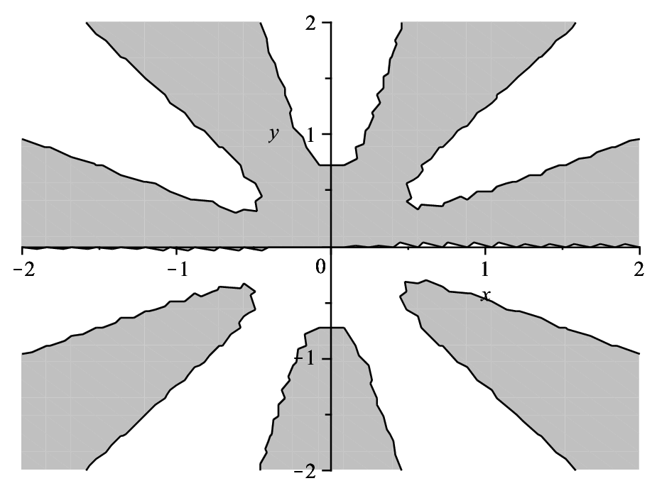
Refer to caption — Figure 8: Contour plot of ${\rm Im\,}\Theta(x^{\frac{1}{2n}}\zeta)$ for $x>0$ large and $n=3$ . The shaded areas indicate where ${\rm Im\,}\Theta(x^{\frac{1}{2n}}\zeta)>0$ . The contour $\widetilde{\Upsilon}$ should lie in the shaded region in the upper half plane and in the white region in the lower half plane.

RH problem for $\widetilde{T}$

(a)

$\widetilde{T}$ is analytic in $\mathbb{C}\setminus\widetilde{\Upsilon}$ .

(b)

The boundary values of $\widetilde{T}$ on $\widetilde{\Upsilon}\setminus\{0\}$ satisfy the jump relations

$\displaystyle\widetilde{T}_{+}(\zeta)$	$\displaystyle=\widetilde{T}_{-}(\zeta)\begin{pmatrix}1&0\\ -ie^{2i\Theta(x^{\frac{1}{2n}}\zeta)}&1\end{pmatrix},\qquad\mbox{for $\zeta\in\left(\widetilde{\Upsilon}_{1}\cup\widetilde{\Upsilon}_{2n+1}\right)\setminus[0,i\delta]$,}$	(4.28)
$\displaystyle\widetilde{T}_{+}(\zeta)$	$\displaystyle=\widetilde{T}_{-}(\zeta)\begin{pmatrix}1&-ie^{-2i\Theta(x^{\frac{1}{2n}}\zeta)}\\ 0&1\end{pmatrix},\qquad\mbox{for $\zeta\in\left(\widetilde{\Upsilon}_{2n+2}\cup\widetilde{\Upsilon}_{4n+2}\right)\setminus[-i\delta,0]$,}$	(4.29)
$\displaystyle\widetilde{T}_{+}(\zeta)$	$\displaystyle=\widetilde{T}_{-}(\zeta)\begin{pmatrix}1&-2ie^{-2i\Theta(x^{\frac{1}{2n}}\zeta)}\\ 0&1\end{pmatrix},\qquad\mbox{for $\zeta\in(-i\delta,0)$,}$	(4.30)
$\displaystyle\widetilde{T}_{+}(\zeta)$	$\displaystyle=\widetilde{T}_{-}(\zeta)\begin{pmatrix}1&0\\ -2ie^{2i\Theta(x^{\frac{1}{2n}}\zeta)}&1\end{pmatrix},\qquad\mbox{for $\zeta\in(0,i\delta)$.}$	(4.31)

(c)

As $\zeta\to\infty$ , we have

$\widetilde{T}(\zeta)=I+\frac{\Psi_{\infty}}{x^{\frac{1}{2n}}\zeta}+{\cal O}(\zeta^{-2}).$ (4.32)

(d)

Near the origin,

\widetilde{T}(\zeta)\begin{pmatrix}1&0\\ \mp i&1\end{pmatrix}={\cal O}\begin{pmatrix}|\zeta|^{\frac{1}{2}}&|\zeta|^{-\frac{1}{2}}\\ |\zeta|^{\frac{1}{2}}&|\zeta|^{-\frac{1}{2}}\end{pmatrix},\qquad\mbox{as $\zeta\to 0,\,\pm{\rm Re\,}\zeta>0$.}

(4.33)

It follows directly from (4.24) and (4.25), (4.26) that, as $x\to+\infty$ , the jump matrices for $\widetilde{T}$ tend to the identity matrix exponentially fast on the jump contour $\widetilde{\Upsilon}$ except near the origin, say in a disk $U_{0}$ of radius $\delta$ centered at $0$ . Moreover, the behaviour of the jump matrices for a fixed $x$ as $\zeta\to\infty$ ensures that the transformation $T\rightarrow\widetilde{T}$ preserves the condition (c).

4.5.2 Local parametrix near the origin

We construct a local parametrix in $U_{0}$ using Bessel functions. The model RH problem we use is different from the one we used in Section 3, although these problems are related.

Bessel model RH problem

Let us define the functions $M_{1}$ , $M_{2}$ as follows:

		$\displaystyle M_{1}(\lambda)=\frac{1}{2}e^{-i\pi\sigma_{3}/4}\begin{pmatrix}1&i\\ i&1\end{pmatrix}\sqrt{\frac{\pi\lambda}{2}}\begin{pmatrix}-iH_{1}^{(2)}(\lambda)&H_{1}^{(1)}(\lambda)\\ -iH_{0}^{(2)}(\lambda)&H_{0}^{(1)}(\lambda)\end{pmatrix},$	for $\lambda\in\mathbb{C}\setminus\mathbb{R}^{-}$ ,		(4.34)
		$\displaystyle M_{2}(\lambda)=\frac{1}{2}e^{-i\pi\sigma_{3}/4}\begin{pmatrix}1&i\\ i&1\end{pmatrix}\sqrt{\frac{\pi\lambda}{2}}\begin{pmatrix}iH_{1}^{(1)}(\lambda e^{-i\pi})&H_{1}^{(2)}(\lambda e^{-i\pi})\\ -iH_{0}^{(1)}(\lambda e^{-i\pi})&-H_{0}^{(2)}(\lambda e^{-i\pi})\end{pmatrix},$	for $\lambda\in\mathbb{C}\setminus\mathbb{R}^{+}$ ,		(4.35)

where $H_{0}^{(1)}$ and $H_{0}^{(2)}$ again denote Hankel functions, with their branch cuts on the negative real axis. We then have the relations:

	$\displaystyle M_{2}(\lambda)$	$\displaystyle=M_{1}(\lambda)\begin{pmatrix}1&0\\ -2i&1\end{pmatrix},$		for $\lambda$ in the upper half-plane,		(4.36)
	$\displaystyle M_{1}(\lambda)$	$\displaystyle=M_{2}(\lambda)\begin{pmatrix}1&-2i\\ 0&1\end{pmatrix},$		for $\lambda$ in the lower half-plane.		(4.37)

Using the asymptotic properties for the Hankel functions, one verifies that $M_{k}$ has the following asymptotics for $\lambda\to\infty$ :

M_{k}(\lambda)=\left[I+\frac{1}{8\lambda}\begin{pmatrix}-i&-2i\\ 2i&i\end{pmatrix}+{\cal O}(\lambda^{-2})\right]e^{-i\lambda\sigma_{3}},\\ \qquad\mbox{as $\lambda\to\infty$ in sector $\widehat{S}_{k}$,}

(4.38)

with

		$\displaystyle\widehat{S}_{1}=\{\lambda:-\pi+\epsilon<\arg\lambda<\pi-\epsilon\},$		(4.39)
		$\displaystyle\widehat{S}_{2}=\{\lambda:\epsilon<\arg\lambda<2\pi-\epsilon\}.$		(4.40)

We will use $M_{1}$ and $M_{2}$ as ’model functions’ to construct a local approximation to the RH solution $\widetilde{T}$ near the origin.

Construction of the parametrix

We define the parametrix $P$ as follows:

P(\zeta)=\begin{cases}\begin{array}[]{ll}M_{1}(x^{\frac{2n+1}{2n}}f(\zeta))e^{i\Theta(x^{\frac{1}{2n}}\zeta)\sigma_{3}},&\mbox{ for ${\rm Re\,}\zeta>0$, $\zeta\in U_{0}$,}\\ M_{2}(x^{\frac{2n+1}{2n}}f(\zeta))e^{i\Theta(x^{\frac{1}{2n}}\zeta)\sigma_{3}},&\mbox{ for ${\rm Re\,}\zeta<0$, $\zeta\in U_{0}$.}\end{array}\end{cases}

(4.41)

where

f(\zeta)=x^{-\frac{2n+1}{2n}}\Theta(x^{\frac{1}{2n}}\zeta).

(4.42)

From (4.24), we have that

f(0)=0,\qquad f^{\prime}(0)=1.

(4.43)

Using the RH conditions for $M_{1}$ and $M_{2}$ we obtain (for sufficiently small $U_{0}$ ):

RH problem for $P$

(a)

$P(\zeta)$ is analytic in $U_{0}\setminus\widetilde{\Upsilon}$ .

(b)

$P$ satisfies the following jump relations on $U_{0}\cap\widetilde{\Upsilon}$ :

	$\displaystyle P_{+}(\zeta)$	$\displaystyle=P_{-}(\zeta)\begin{pmatrix}1&0\\ -2ie^{2i\Theta(x^{\frac{1}{2n}}\zeta)}&1\end{pmatrix},$		for $\zeta\in U_{0}\cap[0,i\delta]$ ,		(4.44)
	$\displaystyle P_{+}(\zeta)$	$\displaystyle=P_{-}(\zeta)\begin{pmatrix}1&-2ie^{-2i\Theta(x^{\frac{1}{2n}}\zeta)}\\ 0&1\end{pmatrix},$		for $\zeta\in U_{0}\cap[-i\delta,0]$ .		(4.45)

(c)

At the boundary $\partial U_{0}$ of $U_{0}$ as $x\to+\infty$ ,

P(\zeta)=I+\frac{1}{8x^{\frac{2n+1}{2n}}f(\zeta)}\begin{pmatrix}-i&-2i\\ 2i&i\end{pmatrix}+{\cal O}\left(x^{-\frac{2n+1}{n}}\right),

(4.46)

(d)

Near the origin,

P(\zeta)\begin{pmatrix}1&0\\ \mp i&1\end{pmatrix}={\cal O}\begin{pmatrix}|\zeta|^{\frac{1}{2}}&|\zeta|^{-\frac{1}{2}}\\ |\zeta|^{\frac{1}{2}}&|\zeta|^{-\frac{1}{2}}\end{pmatrix},\qquad\mbox{as $\zeta\to 0,\,\pm{\rm Re\,}\zeta>0$.}

(4.47)

The local condition (d) follows from the behavior of Hankel functions as $\lambda\to 0$ .

Note that the outside parametrix is simply given by the identity matrix since, away from $0$ , the jump matrices for $\widetilde{T}$ tend to $I$ everywhere.

4.5.3 Final RH problem and asymptotics for $q(x)$ as $x\to+\infty$

Figure 9: Contour

\Sigma_{R}

Let us define

		$\displaystyle R(\zeta)=\widetilde{T}(\zeta)P(\zeta)^{-1}$		for $\zeta\in U_{0}$ ,		(4.48)
		$\displaystyle R(\zeta)=\widetilde{T}(\zeta),$		for $\zeta\in\mathbb{C}\setminus U_{0}$ .		(4.49)

From the behavior of $\widetilde{T}$ and $P$ near the origin it follows that $R$ has a removable singularity at $0$ . The function $R$ satisfies a RH problem with jump matrices which are uniformly close to the identity matrix.

RH problem for $R$

(a)

$R$ is analytic in $\mathbb{C}\setminus\Sigma_{R}$ , with $\Sigma_{R}$ as shown in Figure 9.

(b)

$R$ satisfies the jump relations $R_{+}=R_{-}v_{R}$ on $\Sigma_{R}$ , with

		$\displaystyle v_{R}(\zeta)=P(\zeta),$		for $\zeta\in\partial U_{0}$ ,		(4.50)
		$\displaystyle v_{R}(\zeta)=v_{T}(\zeta),$		for $\zeta\in\Sigma_{R}\setminus\overline{U_{0}}$ .		(4.51)

Outside $\overline{U}_{0}$ , we have already observed that

v_{R}(\zeta)=v_{T}(\zeta)=I+{\cal O}(e^{-cx^{\frac{2n+1}{2n}}}),\qquad\mbox{ as $x\to+\infty$.}

For $\zeta\in\partial U_{0}$ , we obtain from (4.46) that in the limit as $x\to+\infty$ ,

v_{R}(\zeta)=I+\frac{v_{1}(\zeta)}{x^{\frac{2n+1}{2n}}}+{\cal O}\left(x^{-\frac{2n+1}{n}}\right),\qquad v_{1}(\zeta)=\frac{1}{8f(\zeta)}\begin{pmatrix}-i&-2i\\ 2i&i\end{pmatrix}.

(4.52)

This situation is similar to the one in Section 3.5, and we conclude in exactly the same way that

R(\zeta)=I+\frac{R_{1}(\zeta)}{x^{\frac{2n+1}{2n}}}+{\cal O}(x^{-\frac{2n+1}{n}}),\qquad\mbox{ as $x\to+\infty$},

(4.53)

with

R_{1}(\zeta)=\frac{1}{\zeta}{\rm Res}(v_{1};0)=\frac{1}{8\zeta}\begin{pmatrix}-i&-2i\\ 2i&i\end{pmatrix},\qquad\mbox{ for $\zeta\in\mathbb{C}\setminus\overline{U}_{0}$.}

Using the fact that $\widetilde{T}(\zeta)=R(\zeta)$ for $\zeta\in\mathbb{C}\setminus\overline{U}_{0}$ and (4.32), we obtain

\Psi_{\infty}=\frac{1}{8x}\begin{pmatrix}-i&-2i\\ 2i&i\end{pmatrix}+{\cal O}(x^{-\frac{4n+1}{2n}})\qquad\mbox{ as $x\to+\infty$},

(4.54)

so that by (4.12),

q(x;\tau_{1},\ldots,\tau_{n-1})=\frac{1}{2x}+{\cal O}(x^{-\frac{4n+1}{2n}})\qquad\mbox{ as $x\to+\infty$},

(4.55)

which proves part of Theorem 1.8 (equation (1.36).

For later use in Section 5, consider

E(\zeta)\equiv{1\over\sqrt{2}}\begin{pmatrix}1&0\cr-q(x)&1\end{pmatrix}\zeta^{-\frac{1}{4}\sigma_{3}}\begin{pmatrix}1&1\\ -1&1\end{pmatrix}\Psi(i\zeta^{\frac{1}{2}})e^{-\frac{1}{4}\pi i\sigma_{3}}\begin{pmatrix}1&-{1\over 2\pi i}\ln\zeta\\ 0&1\end{pmatrix}

(4.56)

with the principal branch of the root and the logarithm (the branch cut is $(-\infty,0)$ ). We will need to know the asymptotics of $E_{0,11}=\lim_{\zeta\searrow 0}E_{11}(\zeta,x,\tau_{1},\dots,\tau_{n-1})$ as $x\to+\infty$ . The $\zeta$ -limit here is taken so that $u=i\zeta^{1/2}$ tends to zero along $(0,+i\infty)$ . We have

E_{0,11}=\frac{e^{-\frac{i\pi}{4}}}{\sqrt{2}}\lim_{\zeta\searrow 0}\zeta^{-1/4}\left[\begin{pmatrix}1&1\\ -1&1\end{pmatrix}\Psi(i\zeta^{1/2})\right]_{11}.

(4.57)

From (4.27), (4.48), and (4.53), we obtain as $x\to+\infty$

E_{0,11}=\frac{e^{-\frac{i\pi}{4}}}{\sqrt{2}}\lim_{\zeta\searrow 0}\zeta^{-1/4}\left[\begin{pmatrix}1&1\\ -1&1\end{pmatrix}\left(I+{\cal O}(x^{-\frac{2n+1}{2n}})\right)P_{-}(ix^{-\frac{1}{2n}}\zeta^{1/2})\begin{pmatrix}1&0\\ -i&1\end{pmatrix}\right]_{11}.

Using the definition of the parametrix (4.41) and the expansions for Hankel functions near the origin, we finally find

E_{0,11}=e^{\frac{-i\pi}{4}}\sqrt{\pi x}(1+o(1)),\qquad\mbox{ as $x\to+\infty$.}

(4.58)

4.5.4 Asymptotics at $+\infty$ for other solutions of the Painlevé II hierarchy

Figure 10: Deformed contour

\widetilde{\Upsilon}

for solutions with

4

non-zero Stokes multipliers

The special solution to ${\rm P}_{{\rm II}}^{(n)}$ which we considered, i.e. the one with Stokes multipliers

		$\displaystyle s_{1}=s_{2n+1}=-i,$		(4.59)
		$\displaystyle s_{2}=s_{3}=\cdots=s_{2n}=0,$		(4.60)

is not the only solution which has the asymptotic behavior given by (4.55). For $n$ odd, any solution for which the Stokes multipliers satisfy the conditions

		$\displaystyle s_{2}=s_{4}=\cdots=s_{2n}=0,$		(4.61)
		$\displaystyle s_{1}+s_{3}+\cdots+s_{2n+1}=-2i,$		(4.62)

shares this behavior at $+\infty$ . These facts can be proved in a very similar way to the proof we gave for our special solution $q$ . The main difference in the steepest descent analysis is a deformation of the jump contour for $T$ to a contour similar to the one shown in Figure 10. If one chooses the curves so that they coincide near $0$ as indicated in Figure 10, the local parametrix near $0$ can be constructed in exactly the same way as in Section 4.5.2. Furthermore, if the contour is chosen so that conditions (4.25), (4.26) hold, the jump matrices for $R$ still show uniform decay.

If some of the ’even’ Stokes multipliers $s_{2},s_{4},\ldots$ are non-zero, it might still be possible to construct the local parametrix, but there is no way to deform the jump contour in such a way that (4.25) remains valid. In the spirit of the steepest descent method for Painlevé equations, this means (see [23] for several examples of this procedure) that one needs to construct a so-called $g$ -function, which leads typically to a RH problem for which the outside parametrix is not the identity matrix, as it was in our analysis. The leading order of the Painlevé transcendent will then be determined by this outside parametrix. This provides a non-rigorous but strong heuristic argument to believe that only the solutions with Stokes multipliers satisfying (4.61)–(4.62) share the asymptotic behavior at $+\infty$ given by (4.55).

4.6 Asymptotics for $q$ at $-\infty$ for $n$ odd

We will now perform a similar analysis for $q(x)$ as $x\to-\infty$ . The main difference with the analysis at $+\infty$ is that the normalization of the RH problem needs to be done in a less obvious way, using a $g$ -function.

4.6.1 Rescaling of the RH problem and deformation of the jump contour

Figure 11: Deformed contour

\widehat{\Upsilon}

Let us first make a rescaling:

T(\zeta)=\Psi(|x|^{\frac{1}{2n}}\zeta),

(4.63)

and choose a deformed jump contour $\widehat{\Upsilon}$ as indicated in Figure 11. We let $\widehat{\Upsilon}_{4n+2}$ and $\widehat{\Upsilon}_{1}$ coincide along $[0,\zeta_{0}]$ and $\widehat{\Upsilon}_{2n+1}$ and $\widehat{\Upsilon}_{2n+2}$ coincide along $[-\zeta_{0},0]$ . Here $\zeta_{0}$ is real and positive, and we will determine the precise value of $\zeta_{0}$ later on. Away from $[-\zeta_{0},\zeta_{0}]$ , we take each ray in the contour to make an angle of $\frac{\pi}{4n+2}$ with the real line. It will become clear later why this deformation is convenient. We now define a matrix $\widehat{T}$ in terms of $T$ , in a similar way as $\widetilde{T}$ was defined in (4.27). Namely, in the region bounded by $\Upsilon_{1}$ , $\widehat{\Upsilon}_{1}$ , and $(0,\zeta_{0})$ , as well as in the region bounded by $\Upsilon_{2n+1}$ , $\widehat{\Upsilon}_{2n+1}$ , and $(-\zeta_{0},0)$ , the function $\hat{T}$ is defined by extending $T$ analytically from $S_{2}$ . In the region bounded by $\Upsilon_{4n+2}$ , $\widehat{\Upsilon}_{4n+2}$ , and $(0,\zeta_{0})$ , as well as in the region bounded by $\Upsilon_{2n+2}$ , $\widehat{\Upsilon}_{2n+2}$ , and $(-\zeta_{0},0)$ , the function $\widehat{T}$ is defined by extending $T$ analytically from $S_{4}$ . In the regions $\widehat{S}_{1}$ , $\widehat{S}_{3}$ , $S_{2}$ and $S_{4}$ , we set $\widehat{T}=T$ .

4.6.2 Construction of the $g$ -function and normalization of the RH problem

In the previous section where we computed asymptotics at $+\infty$ , we used the obvious way to normalize the RH problem, namely, multiplying on the right with $e^{i\Theta(|x|^{\frac{1}{2n}}\zeta)\sigma_{3}}$ . Here we could do this as well, but it would not lead to a RH problem with decaying jump matrices. This is a consequence of the fact that the topology of the set $\{\zeta:{\rm Im\,}\Theta(|x|^{\frac{1}{2n}}\zeta)>0\}$ for negative $x$ is different from that in Figure 8. We will deal with this problem by replacing $\Theta$ by a function $g$ behaving like $\Theta(|x|^{\frac{1}{2n}}\zeta)$ at infinity and such that the set $\{\zeta:{\rm Im\,}g(\zeta)>0\}$ has a convenient topology.

We define $g$ in the form

g(\zeta)=\sum_{j=1}^{n}c_{j}(\zeta^{2}-\zeta_{0}^{2})^{\frac{2j+1}{2}},

(4.64)

so that $g(\zeta)$ is analytic in $\mathbb{C}\setminus[-\zeta_{0},\zeta_{0}]$ .

We fix the constants $c_{j}$ and the branch point $\zeta_{0}>0$ by the requirement that

|x|^{\frac{2n+1}{2n}}g(\zeta)=\Theta(|x|^{\frac{1}{2n}}\zeta)+{\cal O}(\frac{1}{\zeta}),\qquad\mbox{ as $\zeta\to\infty$.}

(4.65)

Expanding this expression as $\zeta\to\infty$ and equating the coefficients at $\zeta^{2n+1},\zeta^{2n-1},\ldots,\zeta^{3}$ gives (after some calculations which make use of the binomial formula and induction) that, as $x\to-\infty$ ,

		$\displaystyle c_{n}=\frac{2^{2n}}{2n+1},$			(4.66)
		$\displaystyle c_{n-m}=\frac{\Gamma(n+\frac{1}{2})}{\Gamma(n-m+\frac{3}{2})}\frac{2^{2n-1}}{m!}\zeta_{0}^{2m}+{\cal O}(\|x\|^{-\frac{1}{n}}),$	$\displaystyle m=1,\ldots,n-1.$		(4.67)

The coefficient at $\zeta$ yields

\zeta_{0}^{2n}=\frac{n!\sqrt{\pi}}{2^{2n}\Gamma(n+\frac{1}{2})}+{\cal O}(|x|^{-\frac{1}{n}})=\frac{n!^{2}}{(2n)!}+{\cal O}(|x|^{-\frac{1}{n}}).

(4.68)

Here the ${\cal O}(|x|^{-\frac{1}{n}})$ can also be computed explicitly by taking into account the terms with $\tau_{j}$ in $\Theta(|x|^{\frac{1}{2n}}\zeta)$ . Note that the rescaling with a factor $|x|^{\frac{1}{2n}}$ in (4.63) was necessary to have branch points $\pm\zeta_{0}$ with a non-zero finite limit as $x\to-\infty$ .

We now establish some useful properties of the function $g(\zeta)$ . First, let $\zeta\in(0,\zeta_{0})$ . Then

|\zeta^{2}-\zeta_{0}^{2}|=\zeta_{0}^{2}z,\quad z\in(0,1).

Note that by (4.66), (4.67), and (4.68),

c_{n-m}\zeta_{0}^{2(n-m)}=\frac{n!\sqrt{\pi}}{2\Gamma(n-m+\frac{3}{2})m!}+{\cal O}(|x|^{-\frac{1}{n}}),\qquad m=0,\dots,n-1,\quad x\to-\infty.

Thus

g_{\pm}(\zeta)=\frac{n!\sqrt{\pi}}{2}\zeta_{0}\sum_{j=1}^{n}\frac{e^{\pm i\pi(2j+1)/2}z^{j+1/2}}{\Gamma(j+3/2)(n-j)!}+{\cal O}(|x|^{-\frac{1}{n}}),\qquad\zeta\in(0,\zeta_{0}).

(4.69)

Therefore,

g_{+}(\zeta)-g_{-}(\zeta)=2g_{+}(\zeta)=i\sqrt{\pi z}n!\zeta_{0}\phi(z)+{\cal O}(|x|^{-\frac{1}{n}}),\qquad\zeta\in(0,\zeta_{0}),\quad z\in(0,1),

(4.70)

where

\phi(z)=\sum_{j=1}^{n}\frac{(-1)^{j}z^{j}}{\Gamma(j+3/2)(n-j)!}.

(4.71)

We need to determine the sign of $\phi(z)$ for $z\in(0,1)$ . We do it by identifying $\phi(z)$ with a Jacobi polynomial. Jacobi polynomials $p^{(\alpha,\beta)}_{k}(x)$ depend on 2 parameters $\alpha$ and $\beta$ , and have several representations in terms of the hypergeometric function $F$ . We will make use of the following 2 of them:

	$\displaystyle p^{(\alpha,\beta)}_{n-1}(x)=\frac{\Gamma(n+\alpha)}{(n-1)!\Gamma(1+\alpha)}F\left(n+\alpha+\beta,-n+1;1+\alpha;{1-x\over 2}\right),$		(4.72)
	$\displaystyle p^{(\alpha,\beta)}_{n-1}(x)=\frac{\Gamma(n+\beta)(x-1)^{n-1}}{2^{n-1}(n-1)!\Gamma(1+\beta)}F\left(1-n-\alpha,-n+1;1+\beta;{x+1\over x-1}\right).$		(4.73)

From the first of these equations we obtain for $\alpha=3/2$ , $\beta=-n-1/2$ :

p^{(3/2,-n-1/2)}_{n-1}(1-2z)=-{\Gamma(n+3/2)\over z}\phi(z).

(4.74)

On the other hand, the second equation for this particular Jacobi polynomial yields

p^{(3/2,-n-1/2)}_{n-1}(1-2z)={2\Gamma(n+3/2)\over\sqrt{\pi}}\sum_{m=0}^{n-1}\frac{z^{n-m-1}(1-z)^{m}}{m!(n-1-m)!(n+1/2-m)},

(4.75)

which is obviously positive for $z\in(0,1)$ . Therefore, it follows by (4.74) that

\phi(z)<0,\qquad z\in(0,1),

(4.76)

and hence, from (4.70),

{\rm Im\,}(g_{+}-g_{-})=2{\rm Im\,}g_{+}<0,\qquad\zeta\in(0,\zeta_{0}),

(4.77)

for sufficiently large $|x|$ depending on $\tau_{j}$ ’s.

If $\zeta\in(-\zeta_{0},0)$ the only difference is that ${}^{\prime\prime}+^{\prime\prime}$ and ${}^{\prime\prime}-^{\prime\prime}$ sides are interchanged and therefore

{\rm Im\,}(g_{+}-g_{-})=2{\rm Im\,}g_{+}>0,\qquad\zeta\in(-\zeta_{0},0).

(4.78)

Moreover, considering the arguments of $\zeta-\zeta_{0}$ and $\zeta+\zeta_{0}$ , we easily conclude that

	$\displaystyle{\rm Im\,}g(\zeta)>0,\qquad\zeta\in\widehat{\Upsilon}_{1}\cup\widehat{\Upsilon}_{2n+1}$		(4.79)
	$\displaystyle{\rm Im\,}g(\zeta)<0,\qquad\zeta\in\widehat{\Upsilon}_{2n+2}\cup\widehat{\Upsilon}_{4n+2}$		(4.80)
	$\displaystyle g_{+}(\zeta)+g_{-}(\zeta)=0,\qquad\zeta\in(-\zeta_{0},\zeta_{0}).$		(4.81)

Note that the inequalities here and in (4.78) hold, as in (4.77), for sufficiently large $|x|$ .

Let us now define

S(\zeta)=\widehat{T}(\zeta)\exp\left\{i|x|^{\frac{2n+1}{2n}}g(\zeta)\sigma_{3}\right\}.

(4.82)

From the $\Psi$ -RH problem we then have

RH problem for $S$

(a)

$S$ is analytic in $\mathbb{C}\setminus\widehat{\Upsilon}$ .

(b)

$S$ satisfies the following jump relations on $\widehat{\Upsilon}\setminus\{0\}$ :

$\displaystyle S_{+}(\zeta)$	$\displaystyle=S_{-}(\zeta)\begin{pmatrix}1&0\\ -i\exp\left\{2i\|x\|^{\frac{2n+1}{2n}}g(\zeta)\right\}&1\end{pmatrix},\qquad\mbox{for $\zeta\in\left(\widehat{\Upsilon}_{1}\cup\widehat{\Upsilon}_{2n+1}\right)\setminus[-\zeta_{0},\zeta_{0}]$,}$	(4.83)
$\displaystyle S_{+}(\zeta)$	$\displaystyle=S_{-}(\zeta)\begin{pmatrix}1&-i\exp\left\{-2i\|x\|^{\frac{2n+1}{2n}}g(\zeta)\right\}\\ 0&1\end{pmatrix},\qquad\mbox{for $\zeta\in\left(\widehat{\Upsilon}_{2n+2}\cup\widehat{\Upsilon}_{4n+2}\right)\setminus[-\zeta_{0},\zeta_{0}]$,}$	(4.84)
$\displaystyle S_{+}(\zeta)$	$\displaystyle=S_{-}(\zeta)\begin{pmatrix}\exp\left\{2i\|x\|^{\frac{2n+1}{2n}}g_{+}(\zeta)\right\}&-i\\ -i&0\end{pmatrix},\qquad\mbox{for $\zeta\in(-\zeta_{0},0)$,}$	(4.85)
$\displaystyle S_{+}(\zeta)$	$\displaystyle=S_{-}(\zeta)\begin{pmatrix}0&-i\\ -i&\exp\left\{-2i\|x\|^{\frac{2n+1}{2n}}g_{+}(\zeta)\right\}\end{pmatrix},\qquad\mbox{for $\zeta\in(0,\zeta_{0})$,}$	(4.86)

(d)

Near the origin,

S(\zeta)=\begin{cases}\begin{array}[]{ll}{\cal O}\begin{pmatrix}|\zeta|^{1/2}&|\zeta|^{-1/2}\\ |\zeta|^{1/2}&|\zeta|^{-1/2}\end{pmatrix},&\mbox{ as $\zeta\to 0$, ${\rm Im\,}\zeta>0$,}\\ {\cal O}\begin{pmatrix}|\zeta|^{-1/2}&|\zeta|^{1/2}\\ |\zeta|^{-1/2}&|\zeta|^{1/2}\end{pmatrix},&\mbox{ as $\zeta\to 0$, ${\rm Im\,}\zeta<0$.}\end{array}\end{cases}

(4.88)

It follows from (4.77)–(4.80) that the jump matrices for $S$ tend exponentially fast to the identity matrix away from the interval $[-\zeta_{0},\zeta_{0}]$ . On $(-\zeta_{0},\zeta_{0})$ , the diagonal entries decay exponentially fast. The condition (c) is also easy to verify.

4.6.3 Parametrix outside $\pm\zeta_{0}$

Ignoring exponentially small jumps and small neighborhoods of the branch points $\pm\zeta_{0}$ , we are led to a problem for a parametrix $P^{(\infty)}$ :

RH problem for $P^{(\infty)}$

(a)

$P^{(\infty)}$ is analytic in $\mathbb{C}\setminus[-\zeta_{0},\zeta_{0}]$ .
(b)

$P^{(\infty)}$ satisfies the following jump relations on $(-\zeta_{0},0)\cup(0,\zeta_{0})$ , with the intervals $(-\zeta_{0},0)$ and $(0,\zeta_{0})$ both oriented away from the origin,

$\displaystyle P^{(\infty)}_{+}(\zeta)$ $\displaystyle=P^{(\infty)}_{-}(\zeta)\begin{pmatrix}0&-i\\ -i&0\end{pmatrix}.$ (4.89)
(c)

At infinity,

$P^{(\infty)}(\zeta)=I+{\cal O}(\zeta^{-1}),\qquad\zeta\to\infty.$ (4.90)

(d)

Near the origin,

P^{(\infty)}(\zeta)=\begin{cases}\begin{array}[]{ll}{\cal O}\begin{pmatrix}|\zeta|^{1/2}&|\zeta|^{-1/2}\\ |\zeta|^{1/2}&|\zeta|^{-1/2}\end{pmatrix},&\mbox{ as $\zeta\to 0$, ${\rm Im\,}\zeta>0$,}\\ {\cal O}\begin{pmatrix}|\zeta|^{-1/2}&|\zeta|^{1/2}\\ |\zeta|^{-1/2}&|\zeta|^{1/2}\end{pmatrix},&\mbox{ as $\zeta\to 0$, ${\rm Im\,}\zeta<0$.}\end{array}\end{cases}

(4.91)

It is easily seen that this problem has a unique solution which can be found as follows. First, let $\widetilde{P}(\zeta)$ satisfy the same conditions (a), (b), and (c) as $P(\zeta)$ , and write it in the form

\widetilde{P}(\zeta)={1\over 2}\begin{pmatrix}1&-1\\ 1&1\end{pmatrix}L(\zeta)\begin{pmatrix}1&1\\ -1&1\end{pmatrix}.

(4.92)

Then $L(\zeta)$ has a jump on $(-\zeta_{0},\zeta_{0})$ with the diagonal jump matrix $\begin{pmatrix}-i&0\\ 0&i\end{pmatrix}$ , and $L(\infty)=I$ . Therefore, considering the 2 scalar RH problems, we immediately obtain a solution

L(\zeta)=a(\zeta)^{\sigma_{3}},\qquad a(\zeta)=\frac{\zeta^{1/2}}{(\zeta^{2}-\zeta_{0}^{2})^{1/4}}.

(4.93)

We assume that the roots are positive on the real axes to the right of the respective branch points, and the cuts go along the real axis to the left. Note that the corresponding $\widetilde{P}(\zeta)$ satisfies the conditions (a), (b), and (c), but not (d). Let us multiply it on the left by the following matrix

A=I+{1\over\zeta}\begin{pmatrix}\alpha&\beta\\ \gamma&\delta\end{pmatrix}

(4.94)

and choose $\alpha,\beta,\gamma,\delta$ so that $A\widetilde{P}(\zeta)$ satisfies (d), and therefore, since the conditions (a,b,c) are not violated, gives the solution $P^{(\infty)}$ we are looking for. A straightforward calculation yields $\alpha=\beta=-i\zeta_{0}/2$ , $\gamma=\delta=i\zeta_{0}/2$ . Thus, we obtain

P^{(\infty)}(\zeta)=\left[I+{i\zeta_{0}\over 2\zeta}\begin{pmatrix}-1&-1\\ 1&1\end{pmatrix}\right]{1\over 2}\begin{pmatrix}1&-1\\ 1&1\end{pmatrix}\left(\frac{\zeta^{1/2}}{(\zeta^{2}-\zeta_{0}^{2})^{1/4}}\right)^{\sigma_{3}}\begin{pmatrix}1&1\\ -1&1\end{pmatrix}.

(4.95)

As $\zeta\to\infty$ , we clearly have

P^{(\infty)}(\zeta)=I+\frac{i\zeta_{0}}{2\zeta}\begin{pmatrix}-1&-1\\ 1&1\end{pmatrix}+{\cal O}(\zeta^{-2}).

(4.96)

The off-diagonal entries in the coefficient at $\zeta^{-1}$ in this expansion will determine the leading order asymptotics for $q(x)$ .

4.6.4 Local parametrices near $-\zeta_{0}$ and $\zeta_{0}$

In the neighborhoods $U$ of $\zeta_{0}$ and $\widetilde{U}$ of $-\zeta_{0}$ , the local parametrices are constructed in terms of Airy function. The analysis is standard, and we only present the result. In $\widetilde{U}$ , we have

P(\zeta)=\hat{E}(\zeta)A\left(|x|^{\frac{2n+1}{3n}}\lambda\right)\exp\left\{i|x|^{\frac{2n+1}{2n}}g(\zeta)\sigma_{3}\right\},\\ \hat{E}(\zeta)=P^{(\infty)}(\zeta){1\over 2i}\begin{pmatrix}1&-i\\ 1&i\end{pmatrix}\left(|x|^{\frac{2n+1}{3n}}\lambda\right)^{\sigma_{3}/4},\qquad\lambda(\zeta)^{3/2}={3\over 2}e^{\mp 3\pi i/2}g(\zeta),

(4.97)

where the minus sign is taken in the upper half-plane, and plus, in the lower. The function $A$ has the following form in the sector between $\widetilde{\Upsilon}_{2n+1}$ and the real-axis-part of the contour:

A(z)=2\sqrt{\pi}\begin{pmatrix}i{\rm Ai\,}(z)&e^{i\pi/3}{\rm Ai\,}(e^{4\pi i/3}z)\\ {d\over dz}{\rm Ai\,}(z)&-ie^{i\pi/3}{d\over dz}{\rm Ai\,}(e^{4\pi i/3}z)\end{pmatrix}

(4.98)

and is constructed in the other sectors using the jump conditions.

We have the crucial properties: $P(\zeta)S(\zeta)^{-1}$ is analytic in $\widetilde{U}$ , and $P(\zeta)P^{(\infty)}(\zeta)^{-1}=I+{\cal O}(|x|^{-\frac{2n+1}{2n}})$ uniformly on $\partial\widetilde{U}$ as $|x|\to\infty$ . The parametrix $P(\zeta)$ for $\zeta\in U$ is obtained using the transformation $\sigma_{1}A(-z)\sigma_{1}$ .

Note that these parametrices do not contribute to the leading-order asymptotics for $q(x)$ .

4.6.5 Final RH problem and asymptotics for $q$ at $-\infty$

Figure 12: Contour for

R

As before we define $R$ by

		$\displaystyle R(\zeta)=S(\zeta)P(\zeta)^{-1}$		for $\zeta\in U\cup\widetilde{U}$ ,		(4.99)
		$\displaystyle R(\zeta)=S(\zeta)P^{(\infty)}(\zeta)^{-1},$		for $\zeta\in\mathbb{C}\setminus(U\cup\widetilde{U})$ ,		(4.100)

so that $R$ satisfies the following RH problem.

RH problem for $R$

(a)

$R$ is analytic in $\mathbb{C}\setminus\Sigma_{R}$ , with $\Sigma_{R}$ as shown in Figure 12.

(b)

$R$ satisfies the jump relations $R_{+}=R_{-}v_{R}$ on $\Sigma_{R}$ , with

		$\displaystyle\hskip-56.9055ptv_{R}(\zeta)=P(\zeta)P^{(\infty)}(\zeta)^{-1},\quad\mbox{ for $\zeta\in\partial U\cup\partial\widetilde{U}$,}$		(4.101)
		$\displaystyle\hskip-56.9055ptv_{R}(\zeta)=P^{(\infty)}(\zeta)v_{S}(\zeta)P^{(\infty)}(\zeta)^{-1},\quad\mbox{ for $\zeta\in\Sigma_{R}\setminus(\overline{U\cup\widetilde{U}}\cup[-\zeta_{0}+\varepsilon,\zeta_{0}-\varepsilon])$,}$		(4.102)
		$\displaystyle\hskip-56.9055ptv_{R}(\zeta)=I+P^{(\infty)}_{-}(\zeta)\begin{pmatrix}0&i\exp\left\{2i\|x\|^{\frac{2n+1}{2n}}g_{+}(\zeta)\right\}\\ 0&0\end{pmatrix}P^{(\infty)}_{-}(\zeta)^{-1},\quad\mbox{ for $\zeta\in(-\zeta_{0}+\varepsilon,0)$,}$		(4.103)
		$\displaystyle\hskip-56.9055ptv_{R}(\zeta)=I+P^{(\infty)}_{-}(\zeta)\begin{pmatrix}0&0\\ i\exp\left\{-2i\|x\|^{\frac{2n+1}{2n}}g_{+}(\zeta)\right\}&0\end{pmatrix}P^{(\infty)}_{-}(\zeta)^{-1},\quad\mbox{ for $\zeta\in(0,\zeta_{0}-\varepsilon)$.}$		(4.104)

where $\varepsilon$ is the radius of the neighborhoods $U$ and $\widetilde{U}$ . Note that, because of $(\ref{RHP S: d-})$ and $(\ref{RHP Pinfty: d-})$ , $R$ is bounded near the origin. From the last sections we recall that $v_{R}=I+{\cal O}(|x|^{-\frac{2n+1}{2n}})$ uniformly on $\Sigma_{R}$ . It follows in a standard way that $R(\zeta)=I+{\cal O}(|x|^{-\frac{2n+1}{2n}})$ uniformly in $\zeta$ as $x\to-\infty$ . Therefore, we obtain from (4.100), (4.96), (4.82), and (4.10) that

\Psi_{\infty}=\frac{i\zeta_{0}}{2}|x|^{1\over 2n}\begin{pmatrix}-1&-1\\ 1&1\end{pmatrix}+{\cal O}(|x|^{-1}),

(4.105)

so that, by (4.12),

q(x)=\zeta_{0}|x|^{\frac{1}{2n}}+{\cal O}(|x|^{-1}),\qquad\mbox{ as $x\to-\infty$},

(4.106)

which, in combination with (4.68), proves the final part of Theorem 1.8.

For later use, we again need asymptotics for $E$ defined by (4.56). In Section 5 we show that $E(\zeta)$ is analytic near the origin, and we can write

E(\zeta)=E_{0}(I+E_{1}\zeta+o(\zeta)).

A similar analysis to the one following (4.56) for $x\to+\infty$ gives

E_{0,11}=o(1),\qquad\mbox{ as $x\to-\infty$}.

(4.107)

and

E_{1,21}=o(1),\qquad\mbox{ as $x\to-\infty$}.

(4.108)

4.6.6 Asymptotics at $-\infty$ for other solutions of the Painlevé II hierarchy

Similarly to the situation at $+\infty$ , the asymptotics at $-\infty$ only do not uniquely fix our special solution of ${\rm P}_{{\rm II}}^{(n)}$ . In a similar way as was shown for the Painlevé II equation itself (see [23]), one has the freedom to choose some of the even Stokes multipliers $s_{2},s_{4},\ldots,s_{2n}$ different from zero without destroying the above RH analysis.

Under the assumption that the even Stokes multipliers are zero, the method works only if the jump contour connects the branch points $\pm\zeta_{0}$ with infinity within every Stokes sector corresponding to a non-zero Stokes multiplier. A simple analysis of $g(\zeta)$ shows that this only leads to decaying jump matrices for the Stokes multipliers $s_{1}$ and $s_{2n+1}$ , so the other odd multipliers should be zero. Recalling Section 4.5.4, we can conjecture that the restriction

s_{2}=s_{3}=\cdots=s_{2n}=0

is needed in order to connect the asymptotics of $q(x)$ at $+\infty$ and $-\infty$ . In order to preserve the symmetry relation (4.21) and thus to have a real solution, the only possibility then is that $s_{1}=s_{2n+1}=-i$ .

Let us stress once again that this is not a proof that the Painlevé solution we discuss is uniquely determined by the reality and by its asymptotics. In principle a different asymptotic analysis of the RH problem could still lead to the same asymptotics for $q$ . However in view of the direct dependence of the leading order asymptotics for $q$ on the outside parametrix, it would be rather surprising if other solutions with the same asymptotics existed.

5 Higher order Painlevé II formula for the Fredholm determinant

In this section, we will relate the $X$ -RH problem for the Fredholm determinant to the $\Psi$ -RH problem for the Painlevé II hierarchy, namely, to the one corresponding to the special solution of ${\rm P}_{{\rm II}}^{(n)}$ we described in the previous section. By (2.17), this will enable us to express the logarithmic derivative of $\det(I-K_{s}^{(k)})$ in terms of the Painlevé II hierarchy and to prove Theorem 1.12.

5.1 RH problem for the Painlevé XXXIV hierarchy and the Fredholm determinant

Let us define the following function $U=U^{(n)}(\zeta;x,\tau_{1},\ldots,\tau_{n-1})$ in terms of the solution $\Psi^{(n)}$ of the RH problem stated in Section 4.3:

U^{(n)}(\zeta)=\frac{1}{\sqrt{2}}\zeta^{-\frac{1}{4}\sigma_{3}}\begin{pmatrix}1&1\\ -1&1\end{pmatrix}\Psi^{(n)}(i\zeta^{\frac{1}{2}};x,\tau_{1},\ldots,\tau_{n-1})e^{-\frac{1}{4}\pi i\sigma_{3}}.

(5.1)

Here we take as usual the branches of the fractional powers which are analytic in $\mathbb{C}\setminus(-\infty,0]$ and positive on $(0,+\infty)$ .

To obtain a RH problem for $U$ from that for $\Psi$ , note first that the $\Psi$ -RH problem is defined in the plane of the variable $u=i\zeta^{1/2}$ . Because of the symmetry $\sigma_{1}\Psi(-u)\sigma_{1}=\Psi(u)$ , it is enough to consider only the half-plane ${\rm Im\,}u\geq 0$ . The function $\zeta=(-iu)^{2}$ maps it onto the whole $\zeta$ -plane. Now it is easy to verify that $U$ satisfies the following conditions.

RH problem for $U$

(a)

$U(\zeta)$ is analytic in $\mathbb{C}\setminus\Sigma$ , where the contour $\Sigma$ is the one shown in Figure 3,

$\Sigma=\Sigma_{1}\cup\Sigma_{2}\cup\Sigma_{3}\cup\{0\}.$ (5.2)

(b)

The boundary values of $U$ satisfy the relations:

	$\displaystyle U_{+}(\zeta)$	$\displaystyle=U_{-}(\zeta)\begin{pmatrix}1&0\\ 1&1\end{pmatrix},$		for $\zeta\in\Sigma_{1}\cup\Sigma_{3}$ ,		(5.3)
	$\displaystyle U_{+}(\zeta)$	$\displaystyle=U_{-}(\zeta)\begin{pmatrix}0&1\\ -1&0\end{pmatrix},$		for $\zeta\in\Sigma_{2}$ .		(5.4)

(c)

As $\zeta\to\infty$ ,

U(\zeta)=\zeta^{-\frac{1}{4}\sigma_{3}}N\left(I+{\cal O}(\zeta^{-\frac{1}{2}})\right)e^{-i\Theta(i\zeta^{\frac{1}{2}})\sigma_{3}},

(5.5)

with $N$ given by (2.13) and $\Theta$ by (4.11).

(d)

As $\zeta\to 0$ ,

$U(\zeta)={\cal O}(|\zeta|^{-1/2}).$ (5.6)

Although we do not use this fact, it is worth noting that the RH problem for $U$ is the RH problem associated to one solution of the $2n$ -th order equation in the Painlevé XXXIV hierarchy.

Our aim is to identify $U=U^{(n)}$ with the RH problem for $X^{(k)}$ from Section 2 if $n=2k+1$ . Let us first identify the parameters $(s,t_{0},\ldots,t_{2k-1})$ for $X$ with the parameters $(x,\tau_{1},\ldots,\tau_{2k})$ for $U$ . We do this by requiring that

\theta(\zeta+s;t_{0},\ldots,t_{2k-1})=i\Theta(i(c\zeta)^{1/2})+{\cal O}(\frac{1}{\zeta}),\qquad\mbox{ as $\zeta\to\infty$,}\qquad c=4^{-\frac{4k+1}{4k+3}},

(5.7)

where $\theta$ is defined in (2.14), and $\Theta$ in (4.19). The value of $c$ follows from comparison of the leading order terms in $\zeta$ for $\theta$ and $\Theta$ . Expanding $\theta(\zeta+s)$ for $\zeta\to\infty$ similarly as in (3.7)-(3.9) for fixed $s$ , we find

\theta(\zeta+s)=\sum_{j=0}^{2k+1}b_{j}\zeta^{\frac{2j+1}{2}}+{\cal O}(\zeta^{-1/2}),

(5.8)

with

b_{j}(s)=\frac{\Gamma(2k+\frac{3}{2})}{\Gamma(j+\frac{3}{2})\Gamma(2k+2-j)}s^{2k+1-j}\\ -\sum_{\ell=j}^{2k-1}(-1)^{\ell}t_{\ell}\frac{\Gamma(\ell+\frac{1}{2})}{\Gamma(j+\frac{3}{2})\Gamma(\ell-j+1)}s^{\ell-j}.

(5.9)

Comparing the same powers of $\zeta$ in (5.7) we obtain that $x=x(s;t_{0},\ldots,t_{2k-1})$ and $\tau_{j}=\tau_{j}(s;t_{0},\ldots,t_{2k-1})$ are given as follows:

		$\displaystyle x(s)=-c^{-1/2}b_{0}(s;t_{0},\ldots,t_{2k-1}),$			(5.10)
		$\displaystyle\tau_{j}(s)=(2j+1)4^{-j}c^{-j-\frac{1}{2}}b_{j}(s;t_{0},\ldots,t_{2k-1}),$	$\displaystyle j=1,\ldots,2k.$		(5.11)

Let us now set

\widehat{X}(\zeta;t_{0},\ldots,t_{2k-1})=c^{\frac{1}{4}\sigma_{3}}U(c(\zeta-s);x,\tau_{1},\ldots,\tau_{2k}),

(5.12)

with $x$ and $\tau_{j}$ given by (5.10) and (5.11). It is easy to verify that $\widehat{X}$ satisfies the jump conditions (2.10)–(2.11) of the RH problem for $X$ , and therefore $\widehat{X}X^{-1}$ is a holomorphic function in $\mathbb{C}\setminus\{0\}$ for any RH solution $X$ . Using (5.7) and the asymptotic behavior of $U$ , we see that also the asymptotic condition (2.12) holds for $\widehat{X}$ and $\widehat{X}X^{-1}$ is bounded at infinity. By (2.15) and (5.6), $\widehat{X}X^{-1}$ can only have a removable singularity at $0$ . Therefore, by Liouville’s theorem, $\widehat{X}X^{-1}$ is a constant matrix, and so $\widehat{X}$ solves the RH problem for $X$ . Since (2.17) holds for any solution of the $X$ -RH problem, we obtain

F(s)=\frac{d}{ds}\ln\det(I-K_{s}^{(k)})=\frac{4^{-\frac{4k+1}{4k+3}}}{2\pi i}\left.\left(U^{-1}(z)U_{z}(z)\right)_{21}\right|_{z\searrow 0}.

(5.13)

5.2 Proof of Theorem 1.12

In order to prove Theorem 1.12, we will consider the $x$ -derivative of $U$ . As already mentioned, the RH problem for $U$ (see Section 5.1) is not uniquely solvable but has a family of solutions of the form

\widehat{U}(\zeta)=\begin{pmatrix}1&0\\ \eta&1\end{pmatrix}U(\zeta),

(5.14)

where $U$ is defined by (5.1), and $\eta$ is independent of $\zeta$ but may depend on $x,\tau_{1},\ldots,\tau_{2k}$ . Although the identity

F(s)=\frac{d}{ds}\ln\det(I-K_{s}^{(k)})=\frac{4^{-\frac{4k+1}{4k+3}}}{2\pi i}\left.\left(\widehat{U}^{-1}(\zeta)\widehat{U}_{\zeta}(\zeta)\right)_{21}\right|_{\zeta\searrow 0},

(5.15)

which we obtained in (5.13), is independent of the choice of $\eta$ , the linear system satisfied by $\widehat{U}$ does depend on $\eta$ . A convenient choice for us is $\eta=-q$ . Then we obtain from (5.1) and (4.1), (4.3) that $U$ satisfies the following differential equation with respect to $x$ (which is one of the equations in the standard Lax pair for Painlevé XXXIV):

\widehat{U}_{x}(\zeta;x)=\begin{pmatrix}0&-1\\ -\zeta-(q_{x}+q^{2})&0\end{pmatrix}\widehat{U}(\zeta;x).

(5.16)

Let us define a function $E$ by the equation

\widehat{U}(\zeta)=E(\zeta)\begin{pmatrix}1&\frac{1}{2\pi i}\ln\zeta\\ 0&1\end{pmatrix}C(\zeta),

(5.17)

where

C(\zeta)=\begin{cases}\begin{array}[]{ll}I,&\mbox{ in region {\rm I},}\\ \begin{pmatrix}1&0\\ -1&1\end{pmatrix},&\mbox{ in region {\rm II},}\\ \begin{pmatrix}1&0\\ 1&1\end{pmatrix},&\mbox{ in region {\rm III}.}\end{array}\end{cases}

(5.18)

The sectors I, II, and III are those indicated in Figure 2 if $s=0$ . Considering the RH problem for $U$ and choosing the branch of the logarithm with the cut along $(-\infty,0)$ , it is easy to verify that (5.17) defines an analytic $E(\zeta)$ in a neighborhood of zero with $\det E=1$ .

Writing a Taylor series for $E$ near 0,

E(\zeta;x)=E_{0}\left(I+E_{1}\zeta+{\cal O}(\zeta^{2})\right),\qquad\mbox{ as $\zeta\to 0$},

(5.19)

we obtain from (5.15) that

\frac{d}{ds}\ln\det(I-K_{s}^{(k)})=Q(x;\tau_{1},\ldots,\tau_{2k}),

(5.20)

with

Q(x;\tau_{1},\ldots,\tau_{2k})=\frac{4^{-\frac{4k+1}{4k+3}}}{2\pi i}E_{1,21}\left(x;\tau_{1},\ldots,\tau_{2k}\right).

(5.21)

Using (5.16) we also find

		$\displaystyle E_{0,x}=\begin{pmatrix}0&-1\\ -(q_{x}+q^{2})&0\end{pmatrix}E_{0},$		(5.22)
		$\displaystyle E_{1,x}=E_{0}^{-1}\begin{pmatrix}0&0\\ -1&0\end{pmatrix}E_{0},$		(5.23)

and thus

E_{1,21,x}=-E_{0,11}^{2}.

(5.24)

In other words,

Q^{\prime}(x)=u(x)^{2},\qquad u(x)=\frac{e^{\frac{i\pi}{4}}}{\sqrt{2\pi}}2^{-\frac{4k+1}{4k+3}}E_{0,11}(x).

(5.25)

We see from (4.108) that $E_{1,21}(-\infty)=0$ . Therefore equations (5.21) and (5.25) imply the formula (1.42).

Using (5.22) we obtain the following second-order differential equation for $u(x)$ :

u^{\prime\prime}(x)=[q_{x}(x)+q^{2}(x)]u(x).

(5.26)

Substituting the asymptotics (4.58) and (4.107) into (5.25), we obtain the boundary conditions (1.45)-(1.46) for $u$ . They determine $u(x)$ uniquely for a given $q(x)$ . Now it is easy to check directly using Theorem 1.8 that $u(x)$ given by (1.43) is the solution of (5.26) satisfying these boundary conditions. This completes the proof of Theorem 1.12.

6 The constant problem

In this last section we discuss the multiplicative constant in the asymptotics of $\det(I-K_{s}^{(k)})$ as $s\to-\infty$ . In contrast to the sine, Airy and Bessel kernel determinants, we do not provide a compact expression for this constant in terms of single integrals of elementary functions. For this reason and for simplicity of the argument, we assume that $k=1$ and $t_{0}=t_{1}=0$ for the rest of this section (a generalization being straightforward). In this case, the expression (1.30) has the form

\ln\det(I-K_{s}^{(1)})=-\frac{5^{2}}{2^{8}\cdot 7}|s|^{7}+\chi^{(1)}-\frac{3}{8}\ln|s|+{\cal O}(|s|^{-2}),\qquad s\to-\infty,

(6.1)

where $\chi^{(1)}$ is the logarithm of the constant in question. Comparing this expression with Theorem 1.12 for $k=1$ , we obtain a representation of the constant in terms of our special solution $q(x)$ of ${\rm P}_{{\rm II}}^{(3)}$ :

\chi^{(1)}=\lim_{s\to-\infty}\left(\frac{5^{2}}{2^{8}\cdot 7}|s|^{7}+\frac{3}{8}\ln|s|\right.\\ \left.-\int_{s}^{+\infty}Q\left[-2^{5/7-3}5t^{3};2^{1/7-2}15t^{2},2^{-3/7}5t\right]dt\right),

(6.2)

which is basically (using (1.42) and (1.43)) a closed expression for $\chi^{(1)}$ in terms of the Painlevé II solution $q$ with $k=1$ .

This is a generalization of a similar formula, expressing $\chi^{(0)}$ in terms of ${\rm P}_{{\rm II}}^{(1)}$ , in the case of the Airy-kernel determinant.

Let us now try to generalize the argument in [17] which led to the simple expression (1.26) for $\chi^{(0)}$ . Consider the kernel (1.2) with $V(x)$ given by

V(x)=4\left(\frac{1}{5}x^{4}-\frac{4}{3}x^{3}+3x^{2}-2x\right)

for the polynomials $p_{k}(x)$ orthogonal with the weight $e^{-nV(x)}$ on the half-axis $(0,+\infty)$ (we choose a half-axis instead of $\mathbb{R}$ , and hence this $V$ instead of (1.4), for convenience only). The corresponding mean eigenvalue density is supported on $[0,2]$ with the $k=1$ type singularity at $x=2$ :

\psi_{V}(x)=\frac{8}{5\pi}x^{1/2}(2-x)^{5/2}\chi_{[0,2]}.

Remark 6.1

Note that, on the half-axis, one can find a potential $V$ of degree $3$ with a singular endpoint. However, this does not simplify the argument below.

We now expect equation (1.15) to hold at the endpoint $b=2$ . To prove the convergence of the determinants (1.15), one would need to obtain global estimates for the polynomials $p_{k}(x)$ (cf. [17, 16]), which should be possible in view of [12]. Note that (1.15) for our $V(x)=\widetilde{V}(x)$ is equivalent to the following:

\lim_{n\to\infty}\frac{D_{n}(2+s/(cn^{2/7}))}{D_{n}(+\infty)}=\det(I-K_{s}^{(1)}),

(6.3)

where

D_{n}(\alpha)={1\over n!}\int_{0}^{\alpha}\cdots\int_{0}^{\alpha}\prod_{0\leq i<j\leq n-1}(x_{i}-x_{j})^{2}\prod_{j=0}^{n-1}e^{-nV(x_{j})}dx_{j}.

(6.4)

In view of (6.1), this formula would provide a representation for $\chi^{(1)}$ in terms of a limit of multiple integrals. It can be however simplified following [17]. Namely, there exists a differential identity for ${d\over d\alpha}\ln D_{n}(\alpha)$ in terms of the polynomials orthogonal with the weight $e^{nV(x)}$ on the interval $(0,\alpha)$ . Analysing the related RH problem, one may be able to obtain a uniform asymptotics for the polynomials, and hence, for ${d\over d\alpha}\ln D_{n}(\alpha)$ in the range $\alpha\in(0,2+s/(cn^{2/7}))$ , $s<s_{0}<0$ for a sufficiently large $|s_{0}|$ , $n>|s_{0}|$ . On the other hand, it is easy to obtain a series expansion for $D_{n}(\alpha)$ for $n$ fixed and $\alpha\to 0$ . Combining these results, one could integrate ${d\over d\alpha}\ln D_{n}(\alpha)$ from $\alpha\to 0$ to $2+s/(cn^{2/7})$ , and therefore one may be able to obtain, as in [17], an expansion for $D_{n}(2+s/(cn^{2/7}))$ as $n\to\infty$ (and $|s|$ sufficiently large) in terms of elementary functions. Thus, the only non-elementary object to enter the expression for $\det(I-K_{s}^{(1)})$ , $s<s_{0}$ , and hence the expression for $\chi^{(1)}$ , would be $D_{n}(+\infty)$ . This would appear to be a final formula for $\chi^{(1)}$ . Indeed, note that in [17], for $\chi^{(0)}$ , the corresponding $D_{n}(+\infty)$ was a Selberg integral and therefore the corresponding formulas simplified to (1.26). In the present case, however, there is no known expression for $D_{n}(+\infty)$ in terms of elementary functions (or a fixed number of integrals thereof). An attempt to derive the asymptotics of $D_{n}(+\infty)$ as $n\to\infty$ by continuing the integration of the differential identity beyond the endpoint $2$ of the measure is likely to produce an expansion involving integrals of Painlevé functions.

Acknowledgements

Tom Claeys is a Postdoctoral Fellow of the Fund for Scientific Research - Flanders (Belgium), and was also supported by Belgian Interuniversity Attraction Pole P06/02, FWO-Flanders project G042709, K.U.Leuven research grant OT/08/33, and by ESF program MISGAM. Alexander Its was supported in part by NSF grant #DMS-0701768 and EPSRC grant #EP/F014198/1. Igor Krasovsky was supported in part by EPSRC grants #EP/E022928/1 and #EP/F014198/1.

References

[1] M. Abramowitz and I.A. Stegun, “ Handbook of mathematical functions”, Dover Publications, New York (1968).
[2] J. Baik, R. Buckingham, and J. Di Franco, Asymptotics of Tracy-Widom distributions and the total integral of a Painlevé II function, Comm. Math. Phys. 280 (2008), 463–497.
[3] J. Baik, P. Deift, and K. Johansson, On the distribution of the length of the longest increasing subsequence of random permutations, J. Amer. Math. Soc. 12 (1999), 1119–1178.
[4] P. Bleher, A. Bolibruch, A. Its, and A. Kapaev, Linearization of the P34 equation of Painlevé-Gambier, unpublished manuscript.
[5] A. Borodin and P. Deift, Fredholm determinants, Jimbo-Miwa-Ueno tau-functions and representation theory, Comm. Pure Appl. Math. 55 (2002), 1160–1230.
[6] M.J. Bowick and E. Brézin, Universal scaling of the tail of the density of eigenvalues in random matrix models, Phys. Lett. B 268 (1991), no. 1, 21–28.
[7] E. Brézin and S. Hikami, Level spacing of random matrices in an external source, Phys. Rev. E 58 (1998), 7176–7185.
[8] E. Brézin, E. Marinari, and G. Parisi, A non-perturbative ambiguity free solution of a string model, Phys. Lett. B 242 (1990), no. 1, 35–38.
[9] Y. Chen, K.J. Eriksen, and C.A. Tracy, Largest eigenvalue distribution in the double scaling limit of matrix models: a Coulomb fluid approach, J. Phys A 28 (1995), L207–L211.
[10] T. Claeys, A.B.J. Kuijlaars, and M. Vanlessen, Multi-critical unitary random matrix ensembles and the general Painlevé II equation, Ann. Math. 167 (2008), 601–642.
[11] T. Claeys and M. Vanlessen, The existence of a real pole-free solution of the fourth order analogue of the Painlevé I equation, Nonlinearity 20 (2007), 1163–1184.
[12] T. Claeys and M. Vanlessen, Universality of a double scaling limit near singular edge points in random matrix models, Comm. Math. Phys. 273 (2007), 499–532.
[13] P.A. Clarkson, N. Joshi, and M. Mazzocco, The Lax pair for the mKdV hierarchy, Séminaires et Congrès 14, Société Mathématique de France, Paris (2007), 53–64.
[14] P.A. Clarkson, N. Joshi, and A. Pickering, Bäcklund transformations for the second Painlevé hierarchy: a modified truncation approach, Inverse Problems 15 (1999), no. 1, 175–187.
[15] P. Deift, “ Orthogonal Polynomials and Random Matrices: A Riemann-Hilbert Approach”, Courant Lecture Notes 3, New York University 1999.
[16] P. Deift, D. Gioev, Universality at the edge of the spectrum for unitary, orthogonal and symplectic ensembles of random matrices, Comm. Pure Appl. Math. 60 (2007), 867–910.
[17] P. Deift, A. Its, and I. Krasovsky, Asymptotics for the Airy-kernel determinant, Comm. Math. Phys. 278 (2008), 643–678.
[18] P. Deift, A. Its, and X. Zhou, A Riemann-Hilbert approach to asymptotic problems arising in the theory of random matrix models, and also in the theory of integrable statistical mechanics, Ann. Math. 146 (1997), 149-235.
[19] P. Deift, T. Kriecherbauer, and K.T-R McLaughlin, New results on the equilibrium measure for logarithmic potentials in the presence of an external field, J. Approx. Theory 95 (1998), 388–475.
[20] P. Deift, T. Kriecherbauer, K.T-R McLaughlin, S. Venakides, and X. Zhou, Uniform asymptotics for polynomials orthogonal with respect to varying exponential weights and applications to universality questions in random matrix theory, Comm. Pure Appl. Math. 52 (1999), 1335–1425.
[21] M. Duits and A.B.J. Kuijlaars, Painlevé I asymptotics for orthogonal polynomials with respect to a varying quartic weight, Nonlinearity 19 (2006), no. 10, 2211–2245.
[22] H. Flaschka and A.C. Newell, Monodromy and spectrum-preserving deformations I, Comm. Math. Phys. 76 (1980), no. 1, 65–116.
[23] A.S. Fokas, A.R. Its, A.A. Kapaev, and V.Yu. Novokshenov, “ Painlevé transcendents: the Riemann-Hilbert approach”, AMS Mathematical Surveys and Monographs 128 (2006).
[24] A.S. Fokas, U. Mugan, and X. Zhou, On the solvability of Painlevé I, III and V, Inverse Problems 8 (1992), no. 5, 757–785.
[25] A.S. Fokas and X. Zhou, On the solvability of Painlevé II and IV, Comm. Math. Phys. 144 (1992), no. 3, 601–622.
[26] S.P. Hastings and J.B. McLeod, A boundary value problem associated with the second Painlevé transcendent and the Korteweg-de Vries equation, Arch. Rational Mech. Anal. 73 (1980), 31–51.
[27] A.R. Its, A.G. Izergin, V.E. Korepin, and N.A. Slavnov, Differential equations for quantum correlation functions, Int. J. Mod. Phys. B 4 (1990), 1003–1037.
[28] A. Its, A. Kuijlaars, and J. Ostensson, Critical edge behavior in unitary random matrix ensembles and the thirty fourth Painlevé transcendent, Internat. Math. Res. Notices 2008 (2008), article ID rnn017, 67 pages.
[29] N. Joshi and A.V. Kitaev, The Dirichlet boundary value problem for real solutions of the first Painlevé equation on segments in non-positive semi-axis, Journal für die Reine und Angewandte Mathematik 583 (2005), 29-86.
[30] N. Joshi and M. Mazzocco, Existence and uniqueness of tri-tronquée solutions of the second Painlevé hierarchy, Nonlinearity 16 (2003), 427–439.
[31] S. Kamvissis, K.D.T-R McLaughlin, and P.D. Miller, “ Semiclassical soliton ensembles for the focusing nonlinear Schrödinger equation”, Ann. Math. Studies 154, Princeton Univ. Press, Princeton (2003).
[32] A.A. Kapaev, Weakly nonlinear solutions of equation $P_{I}^{2}$ , J. Math. Sc. 73 (1995), no. 4, 468–481.
[33] A.A. Kapaev, Quasi-linear Stokes phenomenon for the Painlevé first equation, J. Phys. A 37 (2004), no. 46, 11149–11167.
[34] N.A. Kudryashov, One generalization of the second Painlevé hierarchy, J. Phys. A: Math. Gen. 35 (2002), 93–99.
[35] N.A. Kudryashov and M.B. Soukharev, Uniformization and transcendence of solutions for the first and second Painlevé hierarchies, Phys. Lett. A 237 (1998), no. 4-5, 206–216.
[36] A.B.J. Kuijlaars and K.T-R McLaughlin, Generic behavior of the density of states in random matrix theory and equilibrium problems in the presence of real analytic external fields, Comm. Pure Appl. Math. 53 (2000), 736-785.
[37] A.B.J. Kuijlaars and M. Vanlessen, Universality for eigenvalue correlations from the modified Jacobi unitary ensemble, Internat. Math. Res. Notices 2002 (2002), no. 30, 1575–1600.
[38] M. Mazzocco and M.Y. Mo, The Hamiltonian structure of the second Painlevé hierarchy, Nonlinearity 20 (2007), no. 12, 2845–2882.
[39] C.A. Tracy and H. Widom, Level spacing distributions and the Airy kernel, Comm. Math. Phys. 159 (1994), no. 1, 151–174.

Higher order analogues of the Tracy-Widom distribution and the Painlevé II hierarchy

Abstract

1 Introduction

Remark 1.1

Example 1.2

RH problem for Φ\Phi

Remark 1.3

Remark 1.4

1.1 Statement of results

1.1.1 Large gap asymptotics

Theorem 1.5

Remark 1.6

Example 1.7

1.1.2 The Painlevé II hierarchy

Theorem 1.8

Remark 1.9

Remark 1.10

Remark 1.11

1.1.3 Painlevé expression for the Fredholm determinants

Theorem 1.12

Remark 1.13

Remark 1.14

Remark 1.15

Outline for the rest of the paper

2 Fredholm determinant in terms of a RH solution

RH problem for YY

RH problem for XX

Remark 2.1

Remark 2.2

3 Large gap asymptotics

3.1 Rescaled RH problem

RH problem for TT

3.2 Normalized RH problem

RH problem for SS

3.3 Outside parametrix

RH problem for P(∞)P^{(\infty)}

3.4 Local parametrix

RH problem for PP

3.4.1 Bessel model RH problem

3.4.2 Construction of the local parametrix

3.5 Final transformation

RH problem for RR

3.6 Large gap asymptotics

4 A solution to the Painlevé II hierarchy

4.1 Lax system for the Painlevé II hierarchy

4.2 The RH problem for the Painlevé II hierarchy

Remark 4.1

4.3 Special solution to the Painlevé II hierarchy

RH problem for Ψ\Psi:

Remark 4.2

Remark 4.3

4.4 Smoothness and reality of qq

Lemma 4.4

4.5 Asymptotics for qq at +∞+\infty for nn odd

4.5.1 Rescaling and normalization of the RH problem

RH problem for T~\widetilde{T}

4.5.2 Local parametrix near the origin

Bessel model RH problem

Construction of the parametrix

RH problem for PP

4.5.3 Final RH problem and asymptotics for q⁡(x)q(x) as x→+∞x\to+\infty

RH problem for RR

4.5.4 Asymptotics at +∞+\infty for other solutions of the Painlevé II hierarchy

4.6 Asymptotics for qq at −∞-\infty for nn odd

4.6.1 Rescaling of the RH problem and deformation of the jump contour

4.6.2 Construction of the gg-function and normalization of the RH problem

RH problem for SS

4.6.3 Parametrix outside ±ζ0\pm\zeta_{0}

RH problem for P(∞)P^{(\infty)}

4.6.4 Local parametrices near −ζ0-\zeta_{0} and ζ0\zeta_{0}

4.6.5 Final RH problem and asymptotics for qq at −∞-\infty

RH problem for RR

4.6.6 Asymptotics at −∞-\infty for other solutions of the Painlevé II hierarchy

5 Higher order Painlevé II formula for the Fredholm determinant

5.1 RH problem for the Painlevé XXXIV hierarchy and the Fredholm determinant

RH problem for UU

5.2 Proof of Theorem 1.12

6 The constant problem

Remark 6.1

Acknowledgements

RH problem for $\Phi$

RH problem for $Y$

RH problem for $X$

RH problem for $T$

RH problem for $S$

RH problem for $P^{(\infty)}$

RH problem for $P$

RH problem for $R$

RH problem for $\Psi$ :

4.4 Smoothness and reality of $q$

4.5 Asymptotics for $q$ at $+\infty$ for $n$ odd

RH problem for $\widetilde{T}$

RH problem for $P$

4.5.3 Final RH problem and asymptotics for $q(x)$ as $x\to+\infty$

RH problem for $R$

4.5.4 Asymptotics at $+\infty$ for other solutions of the Painlevé II hierarchy

4.6 Asymptotics for $q$ at $-\infty$ for $n$ odd

4.6.2 Construction of the $g$ -function and normalization of the RH problem

RH problem for $S$

4.6.3 Parametrix outside $\pm\zeta_{0}$

RH problem for $P^{(\infty)}$

4.6.4 Local parametrices near $-\zeta_{0}$ and $\zeta_{0}$

4.6.5 Final RH problem and asymptotics for $q$ at $-\infty$

RH problem for $R$

4.6.6 Asymptotics at $-\infty$ for other solutions of the Painlevé II hierarchy

RH problem for $U$