跳到论文正文
W Papers独立论文阅读器 arXiv:0901.2196 论文正文 计算阅读时间 · 0%
引用这篇论文根据当前论文元数据生成,正式投稿前建议核对。


License: arXiv.org perpetual non-exclusive license
arXiv:0901.2196v2 [math.GT] 16 Jan 2009

The Khovanov width of twisted links and closed 33-braids

Adam Lowrance Address: Department of Mathematics, Louisiana State University
     Baton Rouge, LA 70817, USA
Email address: lowrance@math.lsu.edu
Date: January 15, 2009
Abstract.

Khovanov homology is a bigraded ℤ\mathbb{Z}-module that categorifies the Jones polynomial. The support of Khovanov homology lies on a finite number of slope two lines with respect to the bigrading. The Khovanov width is essentially the largest horizontal distance between two such lines. We show that it is possible to generate infinite families of links with the same Khovanov width from link diagrams satisfying certain conditions. Consequently, we compute the Khovanov width for all closed 3-braids.

1. Introduction

Let L⊂S3L\subset S^{3} be an oriented link. The Khovanov homology of LL, denoted K​h​(L)Kh(L), was introduced by Mikhail Khovanov in [13], and is a bigraded ℤ\mathbb{Z}-module with homological grading ii and polynomial (or Jones) grading jj so that K​h​(L)=⨁i,jK​hi,j​(L)Kh(L)=\bigoplus_{i,j}Kh^{i,j}(L). The graded Euler characteristic of K​h​(L)Kh(L) is the unnormalized Jones polynomial:

(q+q−1)​VL​(q2)=∑i,j(−1)i​rank​K​hi,j​(L)​qj.(q+q^{-1})V_{L}(q^{2})=\sum_{i,j}(-1)^{i}\text{rank}~Kh^{i,j}(L)q^{j}.

The support of K​h​(L)Kh(L) lies on a finite number of slope 2 lines with respect to the bigrading. Therefore, it is convenient to define the δ\delta-grading by δ=j−2​i\delta=j-2i so that K​h​(L)=⨁δK​hδ​(L)Kh(L)=\bigoplus_{\delta}Kh^{\delta}(L). Also, either all the δ\delta-gradings of K​h​(L)Kh(L) are odd, or they all are even. Let δmin\delta_{\text{min}} be the minimum δ\delta-grading where K​h​(L)Kh(L) is nontrivial and δmax\delta_{\text{max}} be the maximum δ\delta-grading where K​h​(L)Kh(L) is nontrivial. Then K​h​(L)Kh(L) is said to be [δmin,δmax][\delta_{\text{min}},\delta_{\text{max}}]-thick, and the Khovanov width of LL is defined as

wK​h​(L)=12​(δmax−δmin)+1.w_{Kh}(L)=\frac{1}{2}(\delta_{\text{max}}-\delta_{\text{min}})+1.

In this paper, we show the following:

  • •

    If a crossing in a link diagram is width-preserving (defined in Section 3), then it can be replaced with an alternating rational tangle and the Khovanov width does not change (Theorem 3.4).

  • •

    We compute the Khovanov width of all closed 3-braids (Theorem 4.10).

  • •

    We determine the Turaev genus of all closed 3-braids, up to an additive error of at most 1.

  • •

    We show that for closed 3-braids the Khovanov width and odd Khovanov width are equal (Corollary 5.5).

The paper is organized as follows. In Section 2, we review some properties of Khovanov homology. In Section 3, we describe the behavior of Khovanov width when a crossing is replaced by an alternating rational tangle. In Section 4, the Khovanov width of any closed 3-braid is computed. Finally, in Section 5 we show that Khovanov width and odd Khovanov width for closed 3-braids are equal.

Acknowledgements. I wish to thank Scott Baldridge, Oliver Dasbach, Mikhail Khovanov, and Peter Ozsváth for many helpful conversations. A portion of the work for this article was done while the author was visiting Columbia University in the Fall of 2008. He thanks the department of mathematics for their hospitality.

2. Khovanov homology background

In this section, we give background material on Khovanov homology. If DD is a diagram for LL, then denote the Khovanov homology of LL by either K​h​(L)Kh(L) or K​h​(D)Kh(D). Similarly, let wK​h​(L)w_{Kh}(L) and wK​h​(D)w_{Kh}(D) equivalently denote the Khovanov width of LL. If 𝔽\mathbb{F} is a field, then let K​h​(L,𝔽)Kh(L;\mathbb{F}) denote K​h​(L)⊗𝔽Kh(L)\otimes\mathbb{F} and wK​h​(L,𝔽)w_{Kh}(L;\mathbb{F}) denote the width of K​h​(L,𝔽)Kh(L;\mathbb{F}).

Let L1L_{1} and L2L_{2} be oriented links, and let CC be a component of L1L_{1}. Denote by ll the linking number of CC with its complement L1−CL_{1}-C. Let L1′L_{1}^{\prime} be the link L1L_{1} with the orientation of CC reversed. Denote the mirror image of L1L_{1} by L1¯\overline{L_{1}} and the disjoint union of L1L_{1} and L2L_{2} by L1⊔L2L_{1}\sqcup L_{2}. The following proposition was proved by Khovanov in [13].

Proposition 2.1 (Khovanov).

For i,j∈ℤi,j\in\mathbb{Z} there are isomorphisms

K​hi,j​(L1′)\displaystyle Kh^{i,j}(L_{1}^{\prime}) ≅\displaystyle\cong K​hi+2​l,j+2​l​(L1),\displaystyle Kh^{i+2l,j+2l}(L_{1}),
K​hi,j​(L1¯,ℚ)\displaystyle Kh^{i,j}(\overline{L_{1}};\mathbb{Q}) ≅\displaystyle\cong K​h−i,−j​(L1,ℚ)\displaystyle Kh^{-i,-j}(L_{1};\mathbb{Q})
Tor​(K​hi,j​(L1¯))\displaystyle\text{Tor}(Kh^{i,j}(\overline{L_{1}})) ≅\displaystyle\cong Tor​(K​h1−i,−j​(L1)), and\displaystyle\text{Tor}(Kh^{1-i,-j}(L_{1})),\text{ and}
K​hi,j​(L1⊔L2)\displaystyle Kh^{i,j}(L_{1}\sqcup L_{2}) ≅\displaystyle\cong ⊕k,m∈ℤ(Khk,m(L1)⊗Khi−k,j−m(L2))⊕\displaystyle\oplus_{k,m\in\mathbb{Z}}(Kh^{k,m}(L_{1})\otimes Kh^{i-k,j-m}(L_{2}))\oplus
⊕k,m∈ℤTor1ℤ(Khk,m(L1),Khi−k+1,j−m(L2))\displaystyle\oplus_{k,m\in\mathbb{Z}}Tor^{\mathbb{Z}}_{1}(Kh^{k,m}(L_{1}),Kh^{i-k+1,j-m}(L_{2}))

Let DD be a diagram for L1L_{1} and D′D^{\prime} be the diagram DD with the component CC reversed. Denote the number of negative crossings in DD by neg(D)(D), where the sign of a crossing is as in Figure 1. Set s=neg​(D)−neg​(D′)s=\text{neg}(D)-\text{neg}(D^{\prime}). Then Proposition 2.1 implies

K​hδ​(D′)\displaystyle Kh^{\delta}(D^{\prime}) ≅\displaystyle\cong K​hδ+s​(D), and\displaystyle Kh^{\delta+s}(D),\text{ and}
K​hδ​(L1¯,ℚ)\displaystyle Kh^{\delta}(\overline{L_{1}};\mathbb{Q}) ≅\displaystyle\cong K​h−δ​(L1,ℚ).\displaystyle Kh^{-\delta}(L_{1};\mathbb{Q}).

In [14], Khovanov introduced the reduced Khovanov homology. For a knot KK, this theory is denoted K​h~​(K)\widetilde{Kh}(K). For links of more than one component, the reduced Khovanov homology depends on a choice of a marked component, and hence is denoted K​h~​(L,C)\widetilde{Kh}(L,C), where CC is the marked component of LL. Similar to the unreduced version, K​h~​(L,C)\widetilde{Kh}(L,C) is a bigraded ℤ\mathbb{Z}-module with homological grading ii and Jones grading jj so that K​h~​(L,C)=⨁i,jK​h~i,j​(L,C)\widetilde{Kh}(L,C)=\bigoplus_{i,j}\widetilde{Kh}^{i,j}(L,C). The graded Euler characteristic of K​h~​(L,C)\widetilde{Kh}(L,C) is the ordinary Jones polynomial:

VL​(q2)=∑i,j(−1)i​rank​K​h~i,j​(L,C)​qj.V_{L}(q^{2})=\sum_{i,j}(-1)^{i}\text{rank}~\widetilde{Kh}^{i,j}(L,C)q^{j}.

As with Khovanov homology, if δ~min\widetilde{\delta}_{\text{min}} is the minimum δ\delta-grading where K​h~​(L,C)\widetilde{Kh}(L,C) is nontrivial and δ~max\widetilde{\delta}_{\text{max}} is the maximum δ\delta-grading where K​h~​(L,C)\widetilde{Kh}(L,C) is nontrivial, then we say that K​h~​(L,C)\widetilde{Kh}(L,C) is [δ~min,δ~max][\widetilde{\delta}_{\text{min}},\widetilde{\delta}_{\text{max}}]-thick. The reduced Khovanov width is defined as wK​h~​(L)=12​(δ~max−δ~min)+1w_{\widetilde{Kh}}(L)=\frac{1}{2}(\widetilde{\delta}_{\text{max}}-\widetilde{\delta}_{\text{min}})+1.

Asaeda and Przytycki [2] show that there is a long exact sequence relating reduced and unreduced Khovanov homology.

Theorem 2.2 (Asaeda-Przytycki).

There is a long exact sequence relating the reduced and unreduced versions of Khovanov homology:

⋯→K​h~i,j+1​(L,C)→K​hi,j​(L)→K​h~i,j−1​(L,C)→K​h~i+1,j+1​(L,C)→⋯\cdots\to\widetilde{Kh}^{i,j+1}(L,C)\to Kh^{i,j}(L)\to\widetilde{Kh}^{i,j-1}(L,C)\to\widetilde{Kh}^{i+1,j+1}(L,C)\to\cdots
Corollary 2.3.

Let LL be a link with marked component CC. Then K​h​(L)Kh(L) is [δmin,δmax][\delta_{\text{min}},\delta_{\text{max}}]-thick if and only if K​h~​(L,C)\widetilde{Kh}(L,C) is [δmin+1,δmax−1][\delta_{\text{min}}+1,\delta_{\text{max}}-1]-thick. Hence wK​h​(L)−1=wK​h~​(L)w_{Kh}(L)-1=w_{\widetilde{Kh}}(L).

Proof.

The long exact sequence of Theorem 2.2 can be rewritten with respect to the δ\delta-grading as

⋯→K​h~δ+1​(L,C)→K​hδ​(L)→K​h~δ−1​(L,C)→K​h~δ−1​(L,C)→⋯.\cdots\to\widetilde{Kh}^{\delta+1}(L,C)\to Kh^{\delta}(L)\to\widetilde{Kh}^{\delta-1}(L,C)\to\widetilde{Kh}^{\delta-1}(L,C)\to\cdots.

Suppose K​h​(L)Kh(L) is [δmin,δmax][\delta_{\text{min}},\delta_{\text{max}}]-thick. Therefore K​h~δ​(L,C)=0\widetilde{Kh}^{\delta}(L,C)=0 for δ>δmax+1\delta>\delta_{\text{max}}+1 and for δ<δmin−1\delta<\delta_{\text{min}}-1.

Suppose K​h~δmax+1​(L,C)\widetilde{Kh}^{\delta_{\text{max}}+1}(L,C) is nontrivial. Then for some ii and jj where j−2​i=δmax+1j-2i=\delta_{\text{max}}+1, the group K​h~i,j​(L,C)\widetilde{Kh}^{i,j}(L,C) is nontrivial. By repeatedly applying the long exact sequence of Theorem 2.2, one sees that K​h~i+k,j+2​k​(L,C)\widetilde{Kh}^{i+k,j+2k}(L,C) is nontrivial for all k≥0k\geq 0. However, the group K​h~δmax+1​(L,C)\widetilde{Kh}^{\delta_{\text{max}}+1}(L,C) is finitely generated. Hence K​h~δmax+1​(L,C)\widetilde{Kh}^{\delta_{\text{max}}+1}(L,C) is trivial. Similarly, one can show that K​h~δmin−1​(L,C)\widetilde{Kh}^{\delta_{\text{min}}-1}(L,C) is also trivial.

The long exact sequence also implies that K​h~δmax−1​(L,C)\widetilde{Kh}^{\delta_{\text{max}}-1}(L,C) and K​h~δmin+1​(L,C)\widetilde{Kh}^{\delta_{\text{min}}+1}(L,C) are nontrivial. Thus K​h~​(L,C)\widetilde{Kh}(L,C) is [δmin+1,δmax−1][\delta_{\text{min}}+1,\delta_{\text{max}}-1]-thick.

Suppose K​h~​(L,C)\widetilde{Kh}(L,C) is [δmin+1,δmax−1][\delta_{\text{min}}+1,\delta_{\text{max}}-1]-thick. Similar to the case above, if either K​hδmin​(L)Kh^{\delta_{\text{min}}}(L) or K​hδmax​(L)Kh^{\delta_{\text{max}}}(L) are trivial, then one can show that K​h~δmin+1​(L,C)\widetilde{Kh}^{\delta_{\text{min}}+1}(L,C) or K​h~δmax−1​(L,C)\widetilde{Kh}^{\delta_{\text{max}}-1}(L,C) respectively are infinitely generated. Hence K​h​(L)Kh(L) is [δmin,δmax][\delta_{\text{min}},\delta_{\text{max}}]-thick. ∎

Corollary 2.3 implies that if CC and C′C^{\prime} are two components of LL, then K​h~​(L,C)\widetilde{Kh}(L,C) is [δ~min,δ~max][\widetilde{\delta}_{\text{min}},\widetilde{\delta}_{\text{max}}]-thick if and only if K​h~​(L,C′)\widetilde{Kh}(L,C^{\prime}) is [δ~min,δ~max][\widetilde{\delta}_{\text{min}},\widetilde{\delta}_{\text{max}}]-thick. Hence, the notation wK​h~​(L)w_{\widetilde{Kh}}(L) is unambiguous.

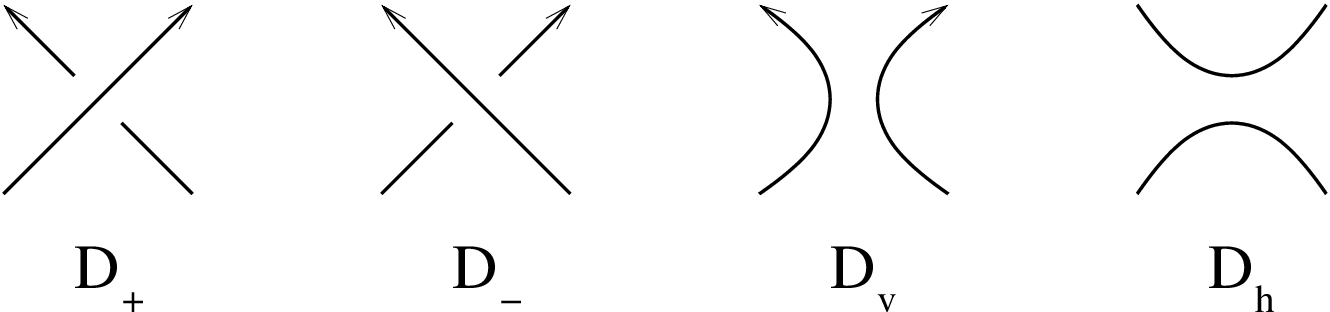
Refer to caption
Figure 1. The links in an oriented resolution. D+D_{+} is a positive crossing, and D−D_{-} is a negative crossing.

Let D+,D−,DvD_{+},D_{-},D_{v} and DhD_{h} be planar diagrams of links that agree outside a neighborhood of a distinguished crossing xx as in Figure 1. Define e=neg​(Dh)−neg​(D+)e=\text{neg}(D_{h})-\text{neg}(D_{+}). There are long exact sequences relating the Khovanov homology of each of these links. Khovanov [13] implicitly describes these sequences, and Viro [25] explicitly states both sequences. The graded versions are taken from Rasmussen [20] and Manolescu-Ozsváth [16].

Theorem 2.4 (Khovanov).

There are long exact sequences

⋯→K​hi−e−1,j−3​e−2​(Dh)→K​hi,j​(D+)→K​hi,j−1​(Dv)→K​hi−e,j−3​e−2​(Dh)→⋯\cdots\to Kh^{i-e-1,j-3e-2}(D_{h})\xrightarrow{}Kh^{i,j}(D_{+})\xrightarrow{}Kh^{i,j-1}(D_{v})\xrightarrow{}Kh^{i-e,j-3e-2}(D_{h})\to\cdots

and

⋯→K​hi,j+1​(Dv)→K​hi,j​(D−)→K​hi−e+1,j−3​e+2​(Dh)→K​hi+1,j+1​(Dv)→⋯.\cdots\to Kh^{i,j+1}(D_{v})\xrightarrow{}Kh^{i,j}(D_{-})\xrightarrow{}Kh^{i-e+1,j-3e+2}(D_{h})\xrightarrow{}Kh^{i+1,j+1}(D_{v})\to\cdots.

When only the δ=j−2​i\delta=j-2i grading is considered, the long exact sequences become

⋯→K​hδ−e​(Dh)→f+δ−eK​hδ​(D+)→g+δK​hδ−1​(Dv)→h+δ−1K​hδ−e−2​(Dh)→⋯\cdots\to Kh^{\delta-e}(D_{h})\xrightarrow{f^{\delta-e}_{+}}Kh^{\delta}(D_{+})\xrightarrow{g^{\delta}_{+}}Kh^{\delta-1}(D_{v})\xrightarrow{h^{\delta-1}_{+}}Kh^{\delta-e-2}(D_{h})\to\cdots

and

⋯→K​hδ+1​(Dv)→f−δ+1K​hδ​(D−)→g−δK​hδ−e​(Dh)→h−δ−eK​hδ−1​(Dv)→⋯\cdots\to Kh^{\delta+1}(D_{v})\xrightarrow{f^{\delta+1}_{-}}Kh^{\delta}(D_{-})\xrightarrow{g^{\delta}_{-}}Kh^{\delta-e}(D_{h})\xrightarrow{h^{\delta-e}_{-}}Kh^{\delta-1}(D_{v})\to\cdots

There are versions of these long exact sequences where Khovanov homology is replaced with reduced Khovanov homology. In the reduced sequences, the gradings are identical to the unreduced sequences.

Refer to caption
Figure 2. The links in an unoriented resolution.

Let DD, D0D_{0} and D1D_{1} be link diagrams differing only in a neighborhood of a crossing xx of DD (as in Figure 2) with associated link types LL, L0L_{0} and L1L_{1} respectively. The set 𝒬\mathcal{Q} of quasi-alternating links is the smallest set of links such that

  • •

    The unknot is in 𝒬\mathcal{Q}.

  • •

    If the link LL has a diagram with a crossing xx such that

    1. (1)

      both of the links, L0L_{0} and L1L_{1} are in 𝒬\mathcal{Q},

    2. (2)

      det(L)=(L)= det(L0)+(L_{0})+det(L1),(L_{1}),

then LL is in 𝒬\mathcal{Q}. We will say that DD is quasi-alternating at xx.

In [15], Lee showed that alternating links have reduced Khovanov width 1. The set of alternating links is a proper subset of the set of quasi-alternating links. Manolescu and Ozsváth [16] use the long exact sequences for reduced Khovanov homology to show that the same result holds for quasi-alternating links.

Theorem 2.5 (Manolescu-Ozsváth).

Let LL be a quasi-alternating link. Then K​h~​(L)\widetilde{Kh}(L) is supported entirely in δ\delta-grading −σ⁡(L)-\sigma(L), where σ⁡(L)\sigma(L) denotes the signature of the link.

Theorem 2.5 together with Corollary 2.3 imply that if LL is quasi-alternating, then K​h​(L)Kh(L) is [−σ⁡(L)−1,−σ⁡(L)+1][-\sigma(L)-1,-\sigma(L)+1]-thick and wK​h​(L)=2w_{Kh}(L)=2.

Theorem 2.4 directly implies the following corollary:

Corollary 2.6.

Let D+,D−,DvD_{+},D_{-},D_{v} and DhD_{h} be as in Figure 1. Suppose K​h​(Dv)Kh(D_{v}) is [vmin,vmax][v_{\text{min}},v_{\text{max}}]-thick and K​h​(Dh)Kh(D_{h}) is [hmin,hmax][h_{\text{min}},h_{\text{max}}]-thick. Then K​h​(D+)Kh(D_{+}) is [δmin+,δmax+][\delta_{\text{min}}^{+},\delta_{\text{max}}^{+}]-thick, and K​h​(D−)Kh(D_{-}) is [δmin−,δmax−][\delta_{\text{min}}^{-},\delta_{\text{max}}^{-}]-thick , where

δmin+={min⁡{vmin+1,hmin+e}if vmin≠hmin+e+1vmin+1if vmin=hmin+e+1 and h+vmin is surjectivevmin−1if vmin=hmin+e+1 and h+vmin is not surjective,\delta^{+}_{\text{min}}=\begin{cases}\min\{v_{\text{min}}+1,h_{\text{min}}+e\}&\text{if $v_{\text{min}}\neq h_{\text{min}}+e+1$}\\ v_{\text{min}}+1&\text{if $v_{\text{min}}=h_{\text{min}}+e+1$ and $h^{v_{\text{min}}}_{+}$ is surjective}\\ v_{\text{min}}-1&\text{if $v_{\text{min}}=h_{\text{min}}+e+1$ and $h^{v_{\text{min}}}_{+}$ is not surjective,}\end{cases}
δmax+={max⁡{vmax+1,hmax+e}if vmin≠hmax+e+1vmax−1if vmax=hmax+e+1 and h+vmax is injectivevmax+1if vmax=hmax+e+1 and h+vmax is not injectve,\delta^{+}_{\text{max}}=\begin{cases}\max\{v_{\text{max}}+1,h_{\text{max}}+e\}&\text{if $v_{\text{min}}\neq h_{\text{max}}+e+1$}\\ v_{\text{max}}-1&\text{if $v_{\text{max}}=h_{\text{max}}+e+1$ and $h^{v_{\text{max}}}_{+}$ is injective}\\ v_{\text{max}}+1&\text{if $v_{\text{max}}=h_{\text{max}}+e+1$ and $h^{v_{\text{max}}}_{+}$ is not injectve,}\end{cases}
δmin−={min⁡{vmin−1,hmin+e}if vmin≠hmin+e−1vmin+1if vmin=hmin+e−1 and h−vmin is surjectivevmin−1if vmin=hmin+e−1 and h−vmin is not surjective,\delta^{-}_{\text{min}}=\begin{cases}\min\{v_{\text{min}}-1,h_{\text{min}}+e\}&\text{if $v_{\text{min}}\neq h_{\text{min}}+e-1$}\\ v_{\text{min}}+1&\text{if $v_{\text{min}}=h_{\text{min}}+e-1$ and $h^{v_{\text{min}}}_{-}$ is surjective}\\ v_{\text{min}}-1&\text{if $v_{\text{min}}=h_{\text{min}}+e-1$ and $h^{v_{\text{min}}}_{-}$ is not surjective,}\end{cases}

and

δmax−={max⁡{vmax−1,hmax+e}if vmax≠hmax+e−1vmax−1if vmax=hmax+e−1 and h+vmax is injectivevmax+1if vmax=hmax+e−1 and h+vmax is not injective.\delta^{-}_{\text{max}}=\begin{cases}\max\{v_{\text{max}}-1,h_{\text{max}}+e\}&\text{if $v_{\text{max}}\neq h_{\text{max}}+e-1$}\\ v_{\text{max}}-1&\text{if $v_{\text{max}}=h_{\text{max}}+e-1$ and $h^{v_{\text{max}}}_{+}$ is injective}\\ v_{\text{max}}+1&\text{if $v_{\text{max}}=h_{\text{max}}+e-1$ and $h^{v_{\text{max}}}_{+}$ is not injective.}\end{cases}

3. Twisted Links

3.1. Khovanov width of twisted links

Let τ=C⁡(a1,…,am)\tau=C(a_{1},\dots,a_{m}) be a rational tangle, and let DD be a link diagram with a distinguished crossing xx. Suppose the slopes of the arcs near xx are ±1\pm 1. Define DD twisted at xx by τ\tau to be the diagram obtained by removing xx and inserting τ\tau such that a neighborhood of the rightmost crossing or topmost crossing of τ\tau in DτD_{\tau} looks exactly like a neighborhood of xx in DD. The resulting link diagram is denoted DτD_{\tau}. See Figure 3.

Refer to caption
Figure 3. The diagram DD twisted by C⁡(2,3,4)C(2,3,4) and C⁡(−4)C(-4).

The main result of this section, Theorem 3.4, is a generalization of a proposition proved by Champanerkar and Kofman in [8].

Proposition 3.1 (Champanerkar-Kofman).

Let DD be a link diagram with crossing xx, and let τ\tau be an alternating rational tangle such that DD is twisted at xx by τ\tau. If DD is quasi-alternating at xx, then DτD_{\tau} is quasi-alternating at each crossing of τ\tau.

Let DD be a diagram with crossing xx. Resolve DD at the crossing xx to obtain diagrams DvD_{v} and DhD_{h}. Suppose K​h​(Dv)Kh(D_{v}) is [vmin,vmax][v_{\text{min}},v_{\text{max}}]-thick and K​h​(Dh)Kh(D_{h}) is [hmin,hmax][h_{\text{min}},h_{\text{max}}]-thick. As before, set e=neg​(Dh)−neg​(D+)e=\text{neg}(D_{h})-\text{neg}(D_{+}), where D+D_{+} is the same diagram as DD except if the crossing xx in DD is negative, then it is changed to positive in D+D_{+}. The diagram DD is said to be width-preserving at xx if either of the following conditions hold.

  • •

    If xx is a positive crossing in DD, then both vmin≠hmin+e+1v_{\text{min}}\neq h_{\text{min}}+e+1 and vmax≠hmax+e+1v_{\text{max}}\neq h_{\text{max}}+e+1.

  • •

    If xx is a negative crossing in DD, then both vmin≠hmin+e−1v_{\text{min}}\neq h_{\text{min}}+e-1 and vmax≠hmax+e−1v_{\text{max}}\neq h_{\text{max}}+e-1.

Proposition 3.2.

Let DD be a link diagram with crossing xx. If DD is quasi-alternating at xx, then DD is width-preserving at xx.

Proof.

Suppose DD is quasi-alternating at xx. Let DvD_{v} and DhD_{h} be the two resolutions of DD at xx. Since DD is quasi-alternating at xx, it follows that DvD_{v} and DhD_{h} are also quasi-alternating. Theorem 2.5 implies that K​h~​(D)\widetilde{Kh}(D), K​h~​(Dv)\widetilde{Kh}(D_{v}) and K​h~​(Dh)\widetilde{Kh}(D_{h}) are each supported entirely in one δ\delta-grading. Suppose K​h~​(Dv)\widetilde{Kh}(D_{v}) is supported in δ\delta-grading vv and K​h~​(Dh)\widetilde{Kh}(D_{h}) is supported in δ\delta-grading hh. Corollary 2.2 implies that K​h​(Dv)Kh(D_{v}) is [v−1,v+1][v-1,v+1]-thick and K​h​(Dh)Kh(D_{h}) is [h−1,h+1][h-1,h+1]-thick. Let e=neg​(Dh)−neg​(D+)e=\text{neg}(D_{h})-\text{neg}(D_{+}) where D+D_{+} is the same diagram as DD except if xx is negative in DD, then it is changed to positive in D+D_{+}. Since det​(D)=det​(Dv)+det​(Dh)\text{det}(D)=\text{det}(D_{v})+\text{det}(D_{h}), it follows that the nontrivial parts of K​h~​(D)\widetilde{Kh}(D), K​h~​(Dv)\widetilde{Kh}(D_{v}) and K​h~​(Dh)\widetilde{Kh}(D_{h}) lie in three consecutive spots in the long exact sequence of Theorem 2.4 such that K​h~​(Dv)\widetilde{Kh}(D_{v}) and K​h~​(Dh)\widetilde{Kh}(D_{h}) are not adjacent. Therefore, if xx is positive, then v=h+e−1v=h+e-1, and if xx is negative, then v=h+e+1v=h+e+1. The result follows directly. ∎

Lemma 3.3.

Let DD be an oriented link diagram with crossing xx, and let τ\tau be an alternating rational tangle with exactly two crossings x0x_{0} and x1x_{1}. Let DτD_{\tau} be DD twisted at xx by τ\tau. If DD is width-preserving at xx, then for any orientation, DτD_{\tau} is width-preserving at x0x_{0} and x1x_{1}. Moreover, wK​h​(D)=wK​h​(Dτ)w_{Kh}(D)=w_{Kh}(D_{\tau}).

Proof.

There are two ways to twist DD at cc, either horizontally or vertically. Let τ1=C⁡(2)\tau_{1}=C(2) and τ2=C⁡(−2)\tau_{2}=C(-2).

For each case, it is only necessary to prove the result for one choice of orientations on DD and DτD_{\tau}. Proposition 2.1 implies the result for all other choices of orientations on DD and DτD_{\tau}.

Let DvD_{v} and DhD_{h} be the diagrams obtained by resolving DD at xx, and let DviD^{i}_{v} and DhiD^{i}_{h} be the diagrams obtained by resolving DτD_{\tau} at the crossing xix_{i} for i=0,1i=0,1. Suppose K​h​(Dv)Kh(D_{v}) and K​h​(Dh)Kh(D_{h}) are [vmin,vmax][v_{\text{min}},v_{\text{max}}]-thick and [hmin,hmax][h_{\text{min}},h_{\text{max}}]-thick respectively. Let e=neg​(Dh)−neg​(D+)e=\text{neg}(D_{h})-\text{neg}(D_{+}) where D+D_{+} is the same diagram as DD except if the crossing xx is negative in DD, then it is changed to positive in D+D_{+}. Similarly set ei=neg​(Dhi)−neg​(D+i)e_{i}=\text{neg}(D^{i}_{h})-\text{neg}(D^{i}_{+}) where D+iD^{i}_{+} is the same diagram as DτD_{\tau} except if the crossing xix_{i} is negative in DτD_{\tau}, then it is changed to positive in D+D_{+}.

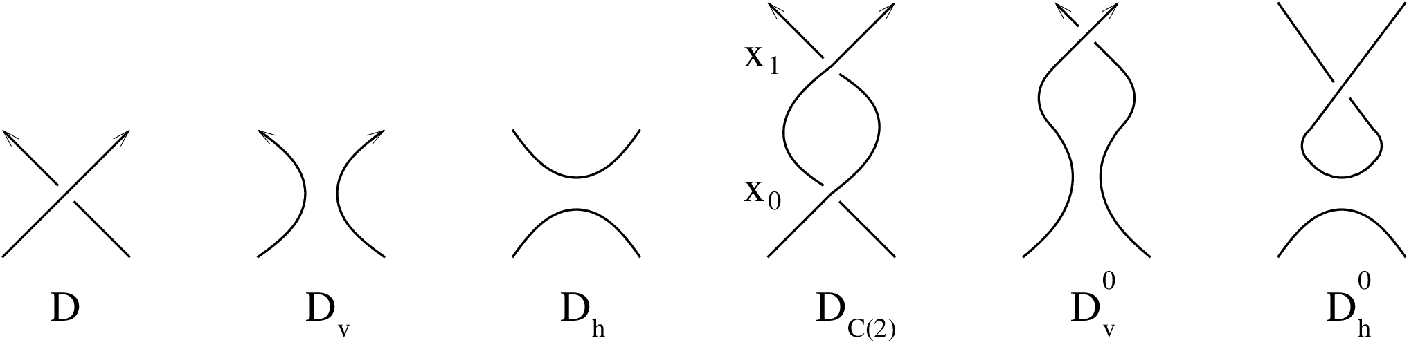
Refer to caption
Figure 4. The resolutions for xx positive and τ=C⁡(2)\tau=C(2).

Suppose xx is positive. Choose the orientation on Dτ1D_{\tau_{1}} given in Figure 4. Also, Figure 4 shows the resolutions Dv0D^{0}_{v} and Dh0D^{0}_{h}.

Observe that xix_{i} is positive in Dτ1D_{\tau_{1}} for i=0,1i=0,1. Corollary 2.6 implies that K​h​(D)Kh(D) is [α,β][\alpha,\beta]-thick where α=min⁡{vmin+1,hmin+e}\alpha=\min\{v_{\text{min}}+1,h_{\text{min}}+e\} and β=max⁡{vmax+1,hmax+e}\beta=\max\{v_{\text{max}}+1,h_{\text{max}}+e\}. The diagrams DviD^{i}_{v} and DD represent the same link, and the diagrams DhD_{h} and DhiD^{i}_{h} represent the same link. Therefore, K​h​(Dvi)Kh(D^{i}_{v}) is [α,β][\alpha,\beta]-thick and K​h​(Dhi)Kh(D^{i}_{h}) is [hmin,hmax][h_{\text{min}},h_{\text{max}}]-thick. The diagram DhiD^{i}_{h} is the same as the diagram DhD_{h} except DhiD^{i}_{h} has one additional negative Reidemeister I twist, and hence neg​(Dhi)=neg​(Dh)+1\text{neg}(D^{i}_{h})=\text{neg}(D_{h})+1. Since the diagrams DD and DviD^{i}_{v} are identical, neg​(D)=neg​(Dvi)\text{neg}(D)=\text{neg}(D^{i}_{v}). Thus ei=e+1e_{i}=e+1. Since DD is width-preserving, it follows that vmin≠hmin+e+1v_{\text{min}}\neq h_{\text{min}}+e+1 and vmax≠hmax+e+1v_{\text{max}}\neq h_{\text{max}}+e+1. Therefore,

hmin+ei+1=hmin+e+2≠α,h_{\text{min}}+e_{i}+1=h_{\text{min}}+e+2\neq\alpha,

and

hmax+ei+1=hmax+e+2≠β.h_{\text{max}}+e_{i}+1=h_{\text{max}}+e+2\neq\beta.

Hence Dτ1D_{\tau_{1}} is width-preserving at xix_{i}. Also, Corollary 2.6 implies that K​h​(Dτ1)Kh(D_{\tau_{1}}) is [α+1,β+1][\alpha+1,\beta+1]-thick, and thus wK​h​(D)=wK​h​(Dτ1)w_{Kh}(D)=w_{Kh}(D_{\tau_{1}}).

Refer to caption
Figure 5. The resolutions for xx positive, τ=C⁡(−2)\tau=C(-2), and with the depicted strands of DD in the same component.

The possible orientations of Dτ2D_{\tau_{2}} depend on whether the strands forming the crossing xx are in the same component of DD or different components of DD. Suppose they are in the same component. Choose the orientation on Dτ2D_{\tau_{2}} given in Figure 5. Also, Figure 5 shows the resolutions Dv0D^{0}_{v} and Dh0D^{0}_{h}.

Observe that xix_{i} is positive in Dτ2D_{\tau_{2}} for i=0,1i=0,1. With suitably chosen orientations, we have

(3.1) neg​(Dv)=neg​(D)=neg​(Dhi),\text{neg}(D_{v})=\text{neg}(D)=\text{neg}(D^{i}_{h}),

and

(3.2) neg​(D+i)=neg​(Dh).\text{neg}(D^{i}_{+})=\text{neg}(D_{h}).

The diagram DviD^{i}_{v} is the same as DvD_{v} except DviD^{i}_{v} has one component reversed and an additional positive Reidemeister I twist. Therefore, Proposition 2.1 implies that K​h​(Dvi)Kh(D^{i}_{v}) is [vmin−e,vmax−e][v_{\text{min}}-e,v_{\text{max}}-e]-thick. Also, equations 3.1 and 3.2 imply that ei=−ee_{i}=-e. The diagram DhiD^{i}_{h} is identical to DD. Therefore, K​h​(Dhi)Kh(D^{i}_{h}) is [α,β][\alpha,\beta]-thick where α=min⁡{vmin+1,hmin+e}\alpha=\min\{v_{\text{min}}+1,h_{\text{min}}+e\} and β=max⁡{vmax+1,hmax+e}\beta=\max\{v_{\text{max}}+1,h_{\text{max}}+e\}. Since DD is width-preserving at xx, we have vmin≠hmin+e+1v_{\text{min}}\neq h_{\text{min}}+e+1 and vmax≠hmax+e+1v_{\text{max}}\neq h_{\text{max}}+e+1. Therefore,

α+ei+1=min⁡{vmin+1,hmin+e}−e+1=min⁡{vmin−e+2,hmin+1}≠vmin−e,\alpha+e_{i}+1=\min\{v_{\text{min}}+1,h_{\text{min}}+e\}-e+1=\min\{v_{\text{min}}-e+2,h_{\text{min}}+1\}\neq v_{\text{min}}-e,

and

β+ei+1=max⁡{vmax+1,hmax+e}−e+1=max⁡{vmax−e+2,hmax+1}≠vmax−e.\beta+e_{i}+1=\max\{v_{\text{max}}+1,h_{\text{max}}+e\}-e+1=\max\{v_{\text{max}}-e+2,h_{\text{max}}+1\}\neq v_{\text{max}}-e.

Thus Dτ2D_{\tau_{2}} is width-preserving at xix_{i}. Moreover, Corollary 2.6 implies that K​h​(Dτ2)Kh(D_{\tau_{2}}) is
[α−e,β−e][\alpha-e,\beta-e]-thick, and hence wK​h​(D)=wK​h​(Dτ2).w_{Kh}(D)=w_{Kh}(D_{\tau_{2}}).

Refer to caption
Figure 6. The resolutions for xx positive, τ=C⁡(−2)\tau=C(-2), and with the depicted strands of DD in different components.

Suppose the strands forming the crossing xx are in different components of the link. Choose the orientation on Dτ2D_{\tau_{2}} given in Figure 6. Also, Figure 6 shows the resolutions Dv0D^{0}_{v} and Dh0D^{0}_{h}.

Observe that xix_{i} is a negative crossing in Dτ2D_{\tau_{2}} for i=0,1i=0,1. Orient DhiD^{i}_{h} so that it represents the same oriented link as DvD_{v}. With a suitably chosen orientation on DhD_{h}, we have

(3.3) neg​(D)=neg​(Dv)=neg​(Dhi),\text{neg}(D)=\text{neg}(D_{v})=\text{neg}(D^{i}_{h}),

and

(3.4) neg​(Dh)+1=neg​(D+i)=neg​(Dvi).\text{neg}(D_{h})+1=\text{neg}(D^{i}_{+})=\text{neg}(D^{i}_{v}).

Equations 3.3 and 3.4 imply that ei=−e−1e_{i}=-e-1. The diagram DviD^{i}_{v} is the same as DD except DviD^{i}_{v} has one component reversed. Equations 3.3 and 3.4 along with Proposition 2.1 imply that K​h​(Dvi)Kh(D^{i}_{v}) is [α−e−1,β−e−1][\alpha-e-1,\beta-e-1]-thick where α=min⁡{vmin+1,hmin+e}\alpha=\min\{v_{\text{min}}+1,h_{\text{min}}+e\} and β=max⁡{vmax+1,hmax+e}\beta=\max\{v_{\text{max}}+1,h_{\text{max}}+e\}. Since DhiD^{i}_{h} and DvD_{v} represent the same oriented link, it follows that K​h​(Dhi)Kh(D^{i}_{h}) is [vmin,vmax][v_{\text{min}},v_{\text{max}}]-thick. Since DD is width-preserving at xx, we have vmin≠hmin+e+1v_{\text{min}}\neq h_{\text{min}}+e+1 and vmax≠hmax+e+1v_{\text{max}}\neq h_{\text{max}}+e+1. Therefore,

α−e−1=min⁡{vmin−e,hmin−1}≠vmin−e−2=vmin+ei−1,\alpha-e-1=\min\{v_{\text{min}}-e,h_{\text{min}}-1\}\neq v_{\text{min}}-e-2=v_{\text{min}}+e_{i}-1,

and

β−e−1=max⁡{vmax−e,hmax−1}≠vmax−e−2=vmax+ei−1.\beta-e-1=\max\{v_{\text{max}}-e,h_{\text{max}}-1\}\neq v_{\text{max}}-e-2=v_{\text{max}}+e_{i}-1.

Thus Dτ2D_{\tau_{2}} is width-preserving at xix_{i}. Moreover, Corollary 2.6 implies that K​h​(Dτ2)Kh(D_{\tau_{2}}) is [α−e−1,β−e−1][\alpha-e-1,\newline \beta-e-1]-thick, and hence wK​h​(D)=wK​h​(Dτ2)w_{Kh}(D)=w_{Kh}(D_{\tau_{2}}),

The case where xx is a negative crossing in DD is proved similarly. ∎

Theorem 3.4.

Let DD be a link diagram with crossing xx, τ\tau be an alternating rational tangle, and DτD_{\tau} be the diagram DD twisted at xx by τ\tau. If DD is width-preserving at xx, then wK​h​(D)=wK​h​(Dτ)w_{Kh}(D)=w_{Kh}(D_{\tau}).

Proof.

Let τ=C⁡(a1,…,am)\tau=C(a_{1},\dots,a_{m}). Since τ\tau is alternating, either ai>0a_{i}>0 for all ii or ai<0a_{i}<0 for all ii. Suppose ai>0a_{i}>0 for all ii. Beginning with the diagram DD and the crossing xx, one can alternate twisting the diagram by C⁡(2)C(2) and C⁡(−2)C(-2). Replacing the appropriate crossings mm times results in the diagram Dτ′D_{\tau^{\prime}} where τ′=C⁡(2,1,…,1)\tau^{\prime}=C(2,1,\dots,1). Lemma 3.3 implies that each crossing in Dτ′D_{\tau^{\prime}} is width-preserving, and wK​h​(D)=wK​h​(Dτ′)w_{Kh}(D)=w_{Kh}(D_{\tau^{\prime}}).

Replace crossings corresponding to the mm-th term in τ′\tau^{\prime} by C⁡(2)C(2) until the resulting diagram is obtained by twisting DD by C⁡(2,1,…,1,am)C(2,1,\dots,1,a_{m}) at xx. Next, replace crossings corresponding to the (m−1)(m-1)-st term in C⁡(2,1,…,1,am)C(2,1,\dots,1,a_{m}) with C⁡(−2)C(-2) until the resulting diagram is obtained by twisting DD by C⁡(2,1,…,1,am−1,am)C(2,1,\dots,1,a_{m-1},a_{m}) at xx. Continue replacing crossings in the tangle by either C⁡(2)C(2) or C⁡(−2)C(-2) until the resulting diagram is obtained by twisting DD by C⁡(a1,…,am)C(a_{1},\dots,a_{m}) at xx. Since at each step, the only tangles used are C⁡(2)C(2) and C⁡(−2)C(-2), Lemma 3.3 implies that wK​h​(D)=wK​h​(Dτ)w_{Kh}(D)=w_{Kh}(D_{\tau}). The case where each ai<0a_{i}<0 is proved similarly. ∎

Refer to caption
Figure 7. The inductive process of Theorem 3.4. At each step, the circled crossing is replaced with either C⁡(2)C(2) or C⁡(−2)C(-2).
Remark 3.5.

Watson [26] proves that wK​h​(Dτ)w_{Kh}(D_{\tau}) is bounded by wK​h​(Dv)w_{Kh}(D_{v}) and wK​h​(Dh)w_{Kh}(D_{h}). By assuming that DD is width-preserving at xx, we are able to strengthen the result and calculate wK​h​(Dτ)w_{Kh}(D_{\tau}).

Suppose DD is an oriented diagram with crossing xx. If DD is twisted at xx by τn=C⁡(n)\tau_{n}=C(n) as in Figure 8, then the assumptions of Theorem 3.4 can be relaxed and a slightly stronger result holds. The following technical result is needed to compute the Khovanov width of closed 3-braids.

Refer to caption
Figure 8. For n>0n>0, twist D+D_{+} by C⁡(n)C(n) and twist D−D_{-} by C⁡(−n)C(-n). Then choose the above orientations for DC⁡(n)D_{C(n)} and DC⁡(−n)D_{C(-n)}.
Proposition 3.6.

Suppose DD is an oriented diagram with crossing xx. Suppose DD is twisted at xx by τn=C⁡(n)\tau_{n}=C(n) as in Figure 8. Let DvD_{v} and DhD_{h} be the two resolutions of DD at xx. Suppose K​h​(Dv)Kh(D_{v}) is [vmin,vmax][v_{\text{min}},v_{\text{max}}]-thick and K​h​(Dh)Kh(D_{h}) is [hmin,hmax][h_{\text{min}},h_{\text{max}}]-thick. Let α±=min⁡{vmin±1,hmin+e}\alpha_{\pm}=\min\{v_{\text{min}}\pm 1,h_{\text{min}}+e\} and β±=max⁡{vmax±1,hmax+e}\beta_{\pm}=\max\{v_{\text{max}}\pm 1,h_{\text{max}}+e\}.

  1. (1)

    Let n>0n>0. Suppose that vmin≠hmin+e+1v_{\text{min}}\neq h_{\text{min}}+e+1. If vmax=hmax+e+1v_{\text{max}}=h_{\text{max}}+e+1, then suppose that there exist integers ii and jj such that j−2​i=vmaxj-2i=v_{\text{max}}, K​hi,j​(Dv)Kh^{i,j}(D_{v}) is nontrivial, and K​hk,l​(Dh)Kh^{k,l}(D_{h}) is trivial for all kk whenever l≤j−3​e−1l\leq j-3e-1. Then K​h​(Dτn)Kh(D_{\tau_{n}}) is [n+α+,n+β+][n+\alpha_{+},n+\beta_{+}]-thick.

  2. (2)

    Let n<0n<0. Suppose that vmax≠hmax+e−1v_{\text{max}}\neq h_{\text{max}}+e-1. If vmin=hmin+e−1v_{\text{min}}=h_{\text{min}}+e-1, then suppose that there exist integers ii and jj such that j−2​i=vminj-2i=v_{\text{min}}, K​hi,j​(Dv)Kh^{i,j}(D_{v}) is nontrivial, and K​hk,l​(Dh)Kh^{k,l}(D_{h}) is trivial for all kk whenever l≥j−3​e−1l\geq j-3e-1. Then K​h​(Dτn)Kh(D_{\tau_{n}}) is [n+α−,n+β−][n+\alpha_{-},n+\beta_{-}]-thick.

Proof.

Let n>0n>0. Since DD is twisted at xx by τn\tau_{n} as in Figure 8, it follows that xx is a positive crossing. If both vmin≠hmin+e+1v_{\text{min}}\neq h_{\text{min}}+e+1 and vmax≠hmax+e+1v_{\text{max}}\neq h_{\text{max}}+e+1, then DD is width-preserving at xx. It follows from the proof of Theorem 3.4 that K​h​(Dτn)Kh(D_{\tau_{n}}) is [n+α+,n+β+][n+\alpha_{+},n+\beta_{+}]-thick.

Suppose vmin≠hmin+e+1v_{\text{min}}\neq h_{\text{min}}+e+1 and vmax=hmax+e+1v_{\text{max}}=h_{\text{max}}+e+1. Thus there exist integers ii and jj such that j−2​i=vmaxj-2i=v_{\text{max}}, K​hi,j​(Dv)Kh^{i,j}(D_{v}) is nontrivial, and K​hk,l​(Dh)Kh^{k,l}(D_{h}) is trivial for all kk and for all l≤j−3​e−1l\leq j-3e-1. Since vmin≠hmin+e+1v_{\text{min}}\neq h_{\text{min}}+e+1, it follows that the minimum δ\delta-grading where K​h​(Dτn)Kh(D_{\tau_{n}}) is nontrivial is n+α+n+\alpha_{+}. We show, by induction on nn, that K​hi,j+n​(Dτn)≅K​hi,j​(Dv)Kh^{i,j+n}(D_{\tau_{n}})\cong Kh^{i,j}(D_{v}). This implies that the maximum δ\delta-grading supporting K​h​(Dτn)Kh(D_{\tau_{n}}) is n+β+n+\beta_{+}.

If n=1n=1, then the long exact sequence of Theorem 2.4 looks like

0→K​hi,j+1​(D)→K​hi,j​(Dv)→K​hi−e,j−3​e−1​(Dh)→⋯.0\to Kh^{i,j+1}(D)\to Kh^{i,j}(D_{v})\to Kh^{i-e,j-3e-1}(D_{h})\to\cdots.

By hypothesis, K​hi−e,j−3​e−1​(Dh)Kh^{i-e,j-3e-1}(D_{h}) is trivial, and hence K​hi,j+1​(D)≅K​hi,j​(Dv)Kh^{i,j+1}(D)\cong Kh^{i,j}(D_{v}).

Suppose, by way of induction, that K​hi,j+n​(Dτn)≅K​hi,j​(Dv)Kh^{i,j+n}(D_{\tau_{n}})\cong Kh^{i,j}(D_{v}). Resolve Dτn+1D_{\tau_{n+1}} at any crossing in τn+1\tau_{n+1} to obtain diagrams Dv′D_{v}^{\prime} and Dh′D_{h}^{\prime}. Let en+1=neg​(Dh′)−neg​(Dτn+1)e_{n+1}=\text{neg}(D_{h}^{\prime})-\text{neg}(D_{\tau_{n+1}}). Since neg​(Dh′)=neg​(Dh)+n\text{neg}(D_{h}^{\prime})=\text{neg}(D_{h})+n and neg​(Dτn+1)=neg​(D)\text{neg}(D_{\tau_{n+1}})=\text{neg}(D), it follows that en+1=e+ne_{n+1}=e+n. Observe that Dv′D_{v}^{\prime} and DτnD_{\tau_{n}} are the same diagram, and Dh′D_{h}^{\prime} and DhD_{h} are diagrams for the same link. Hence the long exact sequence of Theorem 2.4 looks like

0→K​hi,j+n+1​(Dτn+1)→K​hi,j+n​(Dτn)→K​hi−e−n,j−3​e−3​n−1​(Dh)→⋯.0\to Kh^{i,j+n+1}(D_{\tau_{n+1}})\to Kh^{i,j+n}(D_{\tau_{n}})\to Kh^{i-e-n,j-3e-3n-1}(D_{h})\to\cdots.

Since j−3​e−3​n−1≤j−3​e−1j-3e-3n-1\leq j-3e-1, it follows that K​hi−e−n,j−3​e−3​n−1​(Dh)Kh^{i-e-n,j-3e-3n-1}(D_{h}) is trivial. Thus K​hi,j+n+1​(Dτn+1)≅K​hi,j+n​(Dτn)≅K​hi,j​(Dv)Kh^{i,j+n+1}(D_{\tau_{n+1}})\cong Kh^{i,j+n}(D_{\tau_{n}})\cong Kh^{i,j}(D_{v}). Therefore K​h​(Dτn)Kh(D_{\tau_{n}}) is [n+α+,n+β+][n+\alpha_{+},n+\beta_{+}]-thick.

The case where n<0n<0 is proved in a similar fashion using the second sequence from Theorem 2.4. ∎

3.2. The Turaev genus of twisted links

Each link diagram DD has an associated Turaev surface ΣD\Sigma_{D}. Let Γ\Gamma be the plane graph associated to DD. Regard Γ\Gamma as embedded in ℝ2\mathbb{R}^{2} sitting inside ℝ3\mathbb{R}^{3}. Outside the neighborhoods of the vertices of Γ\Gamma is a collection of arcs in the plane. Replace each arc by a band that is perpendicular to the plane. In the neighborhoods of the vertices, place a saddle so that the circles obtained from choosing a 00-resolution at each crossing lie above the plane and so that the circles obtained from choosing a 11-resolution at each crossing lie below the plane (see Figure 9).

Refer to caption
Figure 9. In a neighborhood of each crossing, insert a saddle so that the boundary above the plane corresponds to the 00 resolution and the boundary below the plane corresponds to the 11 resolution.

The resulting surface has a boundary of disjoint circles, with circles corresponding to the all 00-resolution above the plane and circles corresponding to the all 11-resolution below the plane. For each boundary circle, insert a disk to obtain a closed surface ΣD\Sigma_{D} known as the Turaev surface (cf. [23]). The genus of this surface is denoted g⁡(ΣD)g(\Sigma_{D}), and can be calculated by the formula

g⁡(ΣD)=2−s0​(D)−s1​(D)+c⁡(D)2,g(\Sigma_{D})=\frac{2-s_{0}(D)-s_{1}(D)+c(D)}{2},

where c⁡(D)c(D) is the number of crossings in DD and s0​(D)s_{0}(D) and s1​(D)s_{1}(D) are the number of circles appearing in the all 00 and all 11 resolutions of DD respectively. The Turaev genus of a link is defined as

gT​(L)=min⁡{g⁡(ΣD)|D​is a diagram for​L}.g_{T}(L)=\min\{g(\Sigma_{D})~|~D~\text{is a diagram for}~L\}.

The Turaev genus of a link LL is a measure of how far LL is away from being alternating. Specifically, Dasbach et. al. [10] prove the following proposition.

Proposition 3.7 (Dasbach-Futer-Kalfagianni-Lin-Stoltzfus).

A link has Turaev genus 00 if and only if it is alternating.

Also, the Turaev genus of LL gives a bound on the Khovanov width of LL. Manturov [17] and Champanerkar-Kofman-Stoltzfus [9] prove the following inequality.

Proposition 3.8 (Manturov, Champanerkar-Kofman-Stoltzfus).

Let LL be a link. Then

wK​h​(L)−2≤gT​(L).w_{Kh}(L)-2\leq g_{T}(L).

The following proposition is implicit in Champanerkar and Kofman [8], but not explicitly proven.

Proposition 3.9.

Let DD be a link diagram with crossing xx, and let τ\tau be an alternating rational tangle such that DD is twisted by τ\tau at xx. Then g⁡(ΣDτ)=g⁡(ΣD)g(\Sigma_{D_{\tau}})=g(\Sigma_{D}).

Proof.

Suppose τ=C⁡(a1,…,am)\tau=C(a_{1},\dots,a_{m}), where sign​(ai)=sign​(aj)\text{sign}(a_{i})=\text{sign}(a_{j}) for all ii and jj. Let a=∑i=1m|ai|a=\sum_{i=1}^{m}|a_{i}|. The all 0-resolution of DD is the same as the all 0-resolution of DτD_{\tau}, except DτD_{\tau} has an additional kk circles. Similarly, the all 1-resolution of DD is the same as the all 1-resolution of DτD_{\tau}, except DτD_{\tau} has an additional ll circles. Since τ\tau is alternating, it follows that k+l=a−1k+l=a-1. Also, c⁡(Dτ)=c⁡(D)+a−1c(D_{\tau})=c(D)+a-1. Therefore,

g⁡(ΣD)\displaystyle g(\Sigma_{D}) =\displaystyle= 2−s0​(D)−s1​(D)+c⁡(D)2\displaystyle\frac{2-s_{0}(D)-s_{1}(D)+c(D)}{2}
=\displaystyle= 2−(s0​(Dτ)+s1​(Dτ)−(a−1))+c⁡(Dτ)−(a−1)2\displaystyle\frac{2-(s_{0}(D_{\tau})+s_{1}(D_{\tau})-(a-1))+c(D_{\tau})-(a-1)}{2}
=\displaystyle= 2−s0​(Dτ)−s1​(Dτ)+c⁡(Dτ)2\displaystyle\frac{2-s_{0}(D_{\tau})-s_{1}(D_{\tau})+c(D_{\tau})}{2}
=\displaystyle= g⁡(ΣDτ).\displaystyle g(\Sigma_{D_{\tau}}).

∎

In the case where DD is the closure of a braid, there is a particularly nice version of Proposition 3.9. Let w=w⁡(σ1,σ1−1,…,σn−1,σn−1−1)∈Bnw=w(\sigma_{1},\sigma_{1}^{-1},\dots,\sigma_{n-1},\sigma_{n-1}^{-1})\in B_{n} be a word in the braid group, and let DD be the link diagram obtained from taking the closure of ww. Suppose w′w^{\prime} is word in BnB_{n} obtained by replacing σi\sigma_{i} in ww with σik\sigma_{i}^{k} where k>0k>0 or by replacing σi−1\sigma_{i}^{-1} in ww with σik\sigma_{i}^{k} where k<0k<0. Let D′D^{\prime} be the link diagram obtained by taking the braid closure of w′w^{\prime}.

Corollary 3.10.

Let DD and D′D^{\prime} be link diagrams obtained from the closures of the braids ww and w′w^{\prime} respectively. Then g⁡(ΣD)=g⁡(ΣD′)g(\Sigma_{D})=g(\Sigma_{D^{\prime}}).

4. Applications to 3-braids

Closed 3-braids are a rich class of links in which computation of invariants are possible. In [3], Birman and Menasco classify the link types of closed 3-braids. Several papers (Schreier [21], Murasugi [18], and Garside [11]) give algorithms to determine when two 3-braids are conjugate in B3B_{3}. In this paper, we will be interested in Murasugi’s solution to the conjugacy problem.

4.1. Torus Links

Let T⁡(p,q)T(p,q) denote the (p,q)(p,q) torus link. In this subsection, we will determine the Turaev genus and Khovanov width of T⁡(3,q)T(3,q). Turner [24] and Stošić [22] give formulas for the rational Khovanov homology of T⁡(3,q)T(3,q). The following theorem specifies the support of K​h​(T⁡(3,q),ℚ)Kh(T(3,q);\mathbb{Q}) for q≥3q\geq 3. If q≤−3q\leq-3, one can deduce the support from this theorem and the fact that T⁡(3,−q)T(3,-q) is the mirror of T⁡(3,q)T(3,q).

Theorem 4.1 (Stošić, Turner).

Suppose n≥1n\geq 1.

  1. (1)

    The group K​h​(T⁡(3,3​n),ℚ)Kh(T(3,3n);\mathbb{Q}) is [4​n−3,6​n−1][4n-3,6n-1]-thick. Thus wK​h​(T⁡(3,3​n),ℚ)=n+2.w_{Kh}(T(3,3n);\mathbb{Q})=n+2.

  2. (2)

    The group K​h​(T⁡(3,3​n+1),ℚ)Kh(T(3,3n+1);\mathbb{Q}) is [4​n−1,6​n+1][4n-1,6n+1]-thick. Thus wK​h​(T⁡(3,3​n+1),ℚ)=n+2.w_{Kh}(T(3,3n+1);\mathbb{Q})=n+2.

  3. (3)

    The group K​h​(T⁡(3,3​n+2),ℚ)Kh(T(3,3n+2);\mathbb{Q}) is [4​n+1,6​n+3][4n+1,6n+3]-thick. Thus wK​h​(T⁡(3,3​n+2),ℚ)=n+2.w_{Kh}(T(3,3n+2);\mathbb{Q})=n+2.

The following lemma gives several normal forms for braids in B3B_{3} whose closures are torus links. We will use these normal forms to compute the Turaev genus of a (3,q)(3,q) torus link as well as the Turaev genus of many closed 3-braids.

Lemma 4.2.

Let B3B_{3} be the braid group on three strands. Then for any n>1n>1, we have

(σ1​σ2)3\displaystyle(\sigma_{1}\sigma_{2})^{3} =\displaystyle= σ12​σ2​σ12​σ2,\displaystyle\sigma_{1}^{2}\sigma_{2}\sigma_{1}^{2}\sigma_{2},
(σ1​σ2)4\displaystyle(\sigma_{1}\sigma_{2})^{4} =\displaystyle= σ12​σ2​σ13​σ2​σ1,\displaystyle\sigma_{1}^{2}\sigma_{2}\sigma_{1}^{3}\sigma_{2}\sigma_{1},
(σ1​σ2)5\displaystyle(\sigma_{1}\sigma_{2})^{5} =\displaystyle= σ13​σ2​σ13​σ2​σ12,\displaystyle\sigma_{1}^{3}\sigma_{2}\sigma_{1}^{3}\sigma_{2}\sigma_{1}^{2},
(σ1​σ2)3​n\displaystyle(\sigma_{1}\sigma_{2})^{3n} =\displaystyle= σ13​σ2​σ14σ2⋯σ14σ2⏟n−2​σ13​σ2​σ1n+1​σ2,\displaystyle\sigma_{1}^{3}\sigma_{2}\underbrace{\sigma_{1}^{4}\sigma_{2}\cdots\sigma_{1}^{4}\sigma_{2}}_{n-2}\sigma_{1}^{3}\sigma_{2}\sigma_{1}^{n+1}\sigma_{2},
(σ1​σ2)3​n+1\displaystyle(\sigma_{1}\sigma_{2})^{3n+1} =\displaystyle= σ13​σ2​σ14σ2⋯σ14σ2⏟n−2​σ13​σ2​σ1n+2​σ2​σ1, and\displaystyle\sigma_{1}^{3}\sigma_{2}\underbrace{\sigma_{1}^{4}\sigma_{2}\cdots\sigma_{1}^{4}\sigma_{2}}_{n-2}\sigma_{1}^{3}\sigma_{2}\sigma_{1}^{n+2}\sigma_{2}\sigma_{1},\text{ and}
(σ1​σ2)3​n+2\displaystyle(\sigma_{1}\sigma_{2})^{3n+2} =\displaystyle= σ13​σ2​σ14σ2⋯σ14σ2⏟n−1​σ13​σ2​σ1n+1\displaystyle\sigma_{1}^{3}\sigma_{2}\underbrace{\sigma_{1}^{4}\sigma_{2}\cdots\sigma_{1}^{4}\sigma_{2}}_{n-1}\sigma_{1}^{3}\sigma_{2}\sigma_{1}^{n+1}
Proof.

Observe

(σ1​σ2)3\displaystyle(\sigma_{1}\sigma_{2})^{3} =\displaystyle= σ1​σ2​σ1​σ2​σ1​σ2\displaystyle\sigma_{1}\sigma_{2}\sigma_{1}\sigma_{2}\sigma_{1}\sigma_{2}
=\displaystyle= σ12​σ2​σ12​σ2,\displaystyle\sigma_{1}^{2}\sigma_{2}\sigma_{1}^{2}\sigma_{2},
(σ1​σ2)4\displaystyle(\sigma_{1}\sigma_{2})^{4} =\displaystyle= σ12​σ2​σ12​σ2​σ1​σ2\displaystyle\sigma_{1}^{2}\sigma_{2}\sigma_{1}^{2}\sigma_{2}\sigma_{1}\sigma_{2}
=\displaystyle= σ1​σ22​σ1​σ23​σ1, and\displaystyle\sigma_{1}\sigma_{2}^{2}\sigma_{1}\sigma_{2}^{3}\sigma_{1},\text{ and}
(σ1​σ2)5\displaystyle(\sigma_{1}\sigma_{2})^{5} =\displaystyle= σ1​σ2​σ1​σ2​σ1​σ2​σ1​σ2​σ1​σ2\displaystyle\sigma_{1}\sigma_{2}\sigma_{1}\sigma_{2}\sigma_{1}\sigma_{2}\sigma_{1}\sigma_{2}\sigma_{1}\sigma_{2}
=\displaystyle= σ1​σ2​σ1​σ22​σ1​σ2​σ1​σ2​σ1\displaystyle\sigma_{1}\sigma_{2}\sigma_{1}\sigma_{2}^{2}\sigma_{1}\sigma_{2}\sigma_{1}\sigma_{2}\sigma_{1}
=\displaystyle= σ12​σ2​σ1​σ2​σ12​σ2​σ12\displaystyle\sigma_{1}^{2}\sigma_{2}\sigma_{1}\sigma_{2}\sigma_{1}^{2}\sigma_{2}\sigma_{1}^{2}
=\displaystyle= σ13​σ2​σ13​σ2​σ12.\displaystyle\sigma_{1}^{3}\sigma_{2}\sigma_{1}^{3}\sigma_{2}\sigma_{1}^{2}.

The braid relation directly implies the following two relations:

σ1k​σ2​σ1\displaystyle\sigma_{1}^{k}\sigma_{2}\sigma_{1} =\displaystyle= σ2​σ1​σ2k,and\displaystyle\sigma_{2}\sigma_{1}\sigma_{2}^{k},~\text{and}
σ1​σ2​σ1k\displaystyle\sigma_{1}\sigma_{2}\sigma_{1}^{k} =\displaystyle= σ2k​σ1​σ2,\displaystyle\sigma_{2}^{k}\sigma_{1}\sigma_{2},

for k>0k>0. These relations will be used to prove the last three equations in the lemma.

For n>1n>1, we prove that

(σ1​σ2)3​n=σ13​σ2​σ14σ2⋯σ14σ2⏟n−2​σ13​σ2​σ1n+1​σ2(\sigma_{1}\sigma_{2})^{3n}=\sigma_{1}^{3}\sigma_{2}\underbrace{\sigma_{1}^{4}\sigma_{2}\cdots\sigma_{1}^{4}\sigma_{2}}_{n-2}\sigma_{1}^{3}\sigma_{2}\sigma_{1}^{n+1}\sigma_{2}

by induction. Let n=2n=2. Then

(σ1​σ2)6\displaystyle(\sigma_{1}\sigma_{2})^{6} =\displaystyle= σ1​σ2​σ1​σ2​σ1​σ2​σ1​σ2​σ1​σ2​σ1​σ2\displaystyle\sigma_{1}\sigma_{2}\sigma_{1}\sigma_{2}\sigma_{1}\sigma_{2}\sigma_{1}\sigma_{2}\sigma_{1}\sigma_{2}\sigma_{1}\sigma_{2}
=\displaystyle= σ12​σ2​σ1​σ2​σ1​σ2​σ1​σ2​σ12​σ2\displaystyle\sigma_{1}^{2}\sigma_{2}\sigma_{1}\sigma_{2}\sigma_{1}\sigma_{2}\sigma_{1}\sigma_{2}\sigma_{1}^{2}\sigma_{2}
=\displaystyle= σ13​σ2​σ13​σ2​σ13​σ2.\displaystyle\sigma_{1}^{3}\sigma_{2}\sigma_{1}^{3}\sigma_{2}\sigma_{1}^{3}\sigma_{2}.

Suppose, by way of induction, that

(σ1​σ2)3​n=σ13​σ2​σ14σ2⋯σ14σ2⏟n−2​σ13​σ2​σ1n+1​σ2.(\sigma_{1}\sigma_{2})^{3n}=\sigma_{1}^{3}\sigma_{2}\underbrace{\sigma_{1}^{4}\sigma_{2}\cdots\sigma_{1}^{4}\sigma_{2}}_{n-2}\sigma_{1}^{3}\sigma_{2}\sigma_{1}^{n+1}\sigma_{2}.

Then

(σ1​σ2)3​(n+1)\displaystyle(\sigma_{1}\sigma_{2})^{3(n+1)} =\displaystyle= σ13​σ2​σ14σ2⋯σ14σ2⏟n−2​σ13​σ2​σ1n+1​σ2​σ1​σ2​σ1​σ2​σ1​σ2\displaystyle\sigma_{1}^{3}\sigma_{2}\underbrace{\sigma_{1}^{4}\sigma_{2}\cdots\sigma_{1}^{4}\sigma_{2}}_{n-2}\sigma_{1}^{3}\sigma_{2}\sigma_{1}^{n+1}\sigma_{2}\sigma_{1}\sigma_{2}\sigma_{1}\sigma_{2}\sigma_{1}\sigma_{2}
=\displaystyle= σ13​σ2​σ14σ2⋯σ14σ2⏟n−2​σ13​σ2​σ1n+1​σ2​σ1​σ22​σ1​σ22\displaystyle\sigma_{1}^{3}\sigma_{2}\underbrace{\sigma_{1}^{4}\sigma_{2}\cdots\sigma_{1}^{4}\sigma_{2}}_{n-2}\sigma_{1}^{3}\sigma_{2}\sigma_{1}^{n+1}\sigma_{2}\sigma_{1}\sigma_{2}^{2}\sigma_{1}\sigma_{2}^{2}
=\displaystyle= σ13​σ2​σ14σ2⋯σ14σ2⏟n−2​σ13​σ2​σ1n+3​σ2​σ12​σ22\displaystyle\sigma_{1}^{3}\sigma_{2}\underbrace{\sigma_{1}^{4}\sigma_{2}\cdots\sigma_{1}^{4}\sigma_{2}}_{n-2}\sigma_{1}^{3}\sigma_{2}\sigma_{1}^{n+3}\sigma_{2}\sigma_{1}^{2}\sigma_{2}^{2}
=\displaystyle= σ13​σ2​σ14σ2⋯σ14σ2⏟n−2​σ13​σ2​σ1​σ2​σ1​σ2n+2​σ1​σ22\displaystyle\sigma_{1}^{3}\sigma_{2}\underbrace{\sigma_{1}^{4}\sigma_{2}\cdots\sigma_{1}^{4}\sigma_{2}}_{n-2}\sigma_{1}^{3}\sigma_{2}\sigma_{1}\sigma_{2}\sigma_{1}\sigma_{2}^{n+2}\sigma_{1}\sigma_{2}^{2}
=\displaystyle= σ13​σ2​σ14σ2⋯σ14σ2⏟n−2​σ13​σ2​σ1​σ2​σ12​σ2​σ1n+2​σ2\displaystyle\sigma_{1}^{3}\sigma_{2}\underbrace{\sigma_{1}^{4}\sigma_{2}\cdots\sigma_{1}^{4}\sigma_{2}}_{n-2}\sigma_{1}^{3}\sigma_{2}\sigma_{1}\sigma_{2}\sigma_{1}^{2}\sigma_{2}\sigma_{1}^{n+2}\sigma_{2}
=\displaystyle= σ13​σ2​σ14σ2⋯σ14σ2⏟n−2​σ14​σ2​σ13​σ2​σ1n+2​σ2.\displaystyle\sigma_{1}^{3}\sigma_{2}\underbrace{\sigma_{1}^{4}\sigma_{2}\cdots\sigma_{1}^{4}\sigma_{2}}_{n-2}\sigma_{1}^{4}\sigma_{2}\sigma_{1}^{3}\sigma_{2}\sigma_{1}^{n+2}\sigma_{2}.

Hence, for all n>1n>1,

(4.1) (σ1​σ2)3​n=σ13​σ2​σ14σ2⋯σ14σ2⏟n−2​σ13​σ2​σ1n+1​σ2.(\sigma_{1}\sigma_{2})^{3n}=\sigma_{1}^{3}\sigma_{2}\underbrace{\sigma_{1}^{4}\sigma_{2}\cdots\sigma_{1}^{4}\sigma_{2}}_{n-2}\sigma_{1}^{3}\sigma_{2}\sigma_{1}^{n+1}\sigma_{2}.

Equation 4.1 implies

(σ1​σ2)3​n+1\displaystyle(\sigma_{1}\sigma_{2})^{3n+1} =\displaystyle= σ13​σ2​σ14σ2⋯σ14σ2⏟n−2​σ13​σ2​σ1n+1​σ2​σ1​σ2\displaystyle\sigma_{1}^{3}\sigma_{2}\underbrace{\sigma_{1}^{4}\sigma_{2}\cdots\sigma_{1}^{4}\sigma_{2}}_{n-2}\sigma_{1}^{3}\sigma_{2}\sigma_{1}^{n+1}\sigma_{2}\sigma_{1}\sigma_{2}
=\displaystyle= σ13​σ2​σ14σ2⋯σ14σ2⏟n−2​σ13​σ2​σ1n+2​σ2​σ1.\displaystyle\sigma_{1}^{3}\sigma_{2}\underbrace{\sigma_{1}^{4}\sigma_{2}\cdots\sigma_{1}^{4}\sigma_{2}}_{n-2}\sigma_{1}^{3}\sigma_{2}\sigma_{1}^{n+2}\sigma_{2}\sigma_{1}.

Furthermore,

(σ1​σ2)3​n+2\displaystyle(\sigma_{1}\sigma_{2})^{3n+2} =\displaystyle= σ13​σ2​σ14σ2⋯σ14σ2⏟n−2​σ13​σ2​σ1n+2​σ2​σ1​σ1​σ2\displaystyle\sigma_{1}^{3}\sigma_{2}\underbrace{\sigma_{1}^{4}\sigma_{2}\cdots\sigma_{1}^{4}\sigma_{2}}_{n-2}\sigma_{1}^{3}\sigma_{2}\sigma_{1}^{n+2}\sigma_{2}\sigma_{1}\sigma_{1}\sigma_{2}
=\displaystyle= σ13​σ2​σ14σ2⋯σ14σ2⏟n−2​σ13​σ2​σ1​σ2​σ1​σ2n+1​σ1​σ2\displaystyle\sigma_{1}^{3}\sigma_{2}\underbrace{\sigma_{1}^{4}\sigma_{2}\cdots\sigma_{1}^{4}\sigma_{2}}_{n-2}\sigma_{1}^{3}\sigma_{2}\sigma_{1}\sigma_{2}\sigma_{1}\sigma_{2}^{n+1}\sigma_{1}\sigma_{2}
=\displaystyle= σ13​σ2​σ14σ2⋯σ14σ2⏟n−2​σ13​σ2​σ1​σ2​σ12​σ2​σ1n+1\displaystyle\sigma_{1}^{3}\sigma_{2}\underbrace{\sigma_{1}^{4}\sigma_{2}\cdots\sigma_{1}^{4}\sigma_{2}}_{n-2}\sigma_{1}^{3}\sigma_{2}\sigma_{1}\sigma_{2}\sigma_{1}^{2}\sigma_{2}\sigma_{1}^{n+1}
=\displaystyle= σ13​σ2​σ14σ2⋯σ14σ2⏟n−2​σ14​σ2​σ13​σ2​σ1n+1.\displaystyle\sigma_{1}^{3}\sigma_{2}\underbrace{\sigma_{1}^{4}\sigma_{2}\cdots\sigma_{1}^{4}\sigma_{2}}_{n-2}\sigma_{1}^{4}\sigma_{2}\sigma_{1}^{3}\sigma_{2}\sigma_{1}^{n+1}.

∎

Abe and Kishimoto [1] have independently calculated the Turaev genus for the (3,q)-torus links. We give diagrams in closed braid form that minimize Turaev genus, while they have a different approach.

Proposition 4.3.

Suppose q>0q>0. The Turaev genus of T⁡(3,q)T(3,q) and T⁡(3,−q)T(3,-q) is ⌊q/3⌋\lfloor q/3\rfloor.

Proof.

Let DD be the diagram obtained by taking the closure of the normal form for (σ1​σ2)q(\sigma_{1}\sigma_{2})^{q} given in Lemma 4.2. Thus DD is a diagram for T⁡(3,q)T(3,q) and is the closure of a braid in the form

σ1a1σ2b1⋯σ1asσ2bsσ1as+1,\sigma_{1}^{a_{1}}\sigma_{2}^{b_{1}}\cdots\sigma_{1}^{a_{s}}\sigma_{2}^{b_{s}}\sigma_{1}^{a_{s+1}},

where s=⌊q/3⌋+1s=\lfloor q/3\rfloor+1, both ai>0a_{i}>0 and bi>0b_{i}>0 for all 1≤i≤s1\leq i\leq s, and as+1≥0a_{s+1}\geq 0. Let D′D^{\prime} be the diagram obtained by taking the closure of the braid (σ1​σ2)s(\sigma_{1}\sigma_{2})^{s}. Corollary 3.10 implies that g⁡(ΣD)=g⁡(ΣD′)g(\Sigma_{D})=g(\Sigma_{D^{\prime}}). Since c⁡(D′)=2​⌊q/3⌋+2,s0​(D′)=3c(D^{\prime})=2\lfloor q/3\rfloor+2,s_{0}(D^{\prime})=3 and s1​(D′)=1s_{1}(D^{\prime})=1, it follows that g⁡(ΣD′)=⌊q/3⌋g(\Sigma_{D^{\prime}})=\lfloor q/3\rfloor. Proposition 3.8 and Theorem 4.1 imply that the Turaev genus of T⁡(3,q)T(3,q) is greater than or equal to ⌊q/3⌋\lfloor q/3\rfloor. Therefore, gT​(T⁡(3,q))=⌊q/3⌋g_{T}(T(3,q))=\lfloor q/3\rfloor. The genera of the Turaev surfaces for a diagram and its mirror are equal, and hence gT​(T⁡(3,−q))=⌊q/3⌋g_{T}(T(3,-q))=\lfloor q/3\rfloor. ∎

The next corollary follows directly from Theorem 4.1, Proposition 4.3, and Proposition 3.8.

Corollary 4.4.

Suppose n≥1n\geq 1.

  1. (1)

    The group K​h​(T⁡(3,3​n))Kh(T(3,3n)) is [4​n−3,6​n−1][4n-3,6n-1]-thick and the group K​h​(T⁡(3,−3​n))Kh(T(3,-3n)) is
    [−6​n+1,−4​n+3][-6n+1,-4n+3]-thick. Therefore wK​h​(T⁡(3,3​n))=wK​h​(T⁡(3,−3​n))=n+2.w_{Kh}(T(3,3n))=w_{Kh}(T(3,-3n))=n+2.

  2. (2)

    The group K​h​(T⁡(3,3​n+1))Kh(T(3,3n+1)) is [4​n−1,6​n+1][4n-1,6n+1]-thick and the group K​h​(T⁡(3,−3​n−1)CLOSEKh(T(3,-3n-1) is [−6​n−1,−4​n+1][-6n-1,-4n+1]-thick. Therefore wK​h​(T⁡(3,3​n+1))=wK​h​(T⁡(3,−3​n−1)=n+2CLOSE.w_{Kh}(T(3,3n+1))=w_{Kh}(T(3,-3n-1)=n+2.

  3. (3)

    The group K​h​(T⁡(3,3​n+2))Kh(T(3,3n+2)) is [4​n+1,6​n+3][4n+1,6n+3]-thick and the group K​h​(T⁡(3,−3​n−2))Kh(T(3,-3n-2)) is [−6​n−3,−4​n−1][-6n-3,-4n-1]-thick. Therefore wK​h​(T⁡(3,3​n+2))=wK​h​(T⁡(3,−3​n−2))=n+2.w_{Kh}(T(3,3n+2))=w_{Kh}(T(3,-3n-2))=n+2.

4.2. Khovanov width of 3-braids

In this subsection, we determine the Khovanov width of closed 3-braids based upon Murasugi’s classification of closed 3-braids up to conjugation. In [18], Murasugi proves the following:

Theorem 4.5 (Murasugi).

Let w∈B3w\in B_{3} be a braid on three strands, and let h=(σ1​σ2)3h=(\sigma_{1}\sigma_{2})^{3} be a full twist. Let n∈ℤn\in\mathbb{Z}. Then ww is conjugate to exactly one of the following:

  1. (1)

    hnσ1p1σ2−q1⋯σ1psσ2−qsh^{n}\sigma_{1}^{p_{1}}\sigma_{2}^{-q_{1}}\cdots\sigma_{1}^{p_{s}}\sigma_{2}^{-q_{s}} where pi,qip_{i},q_{i} and ss are positive integers.

  2. (2)

    hn​σ2mh^{n}\sigma_{2}^{m} where m∈ℤm\in\mathbb{Z}.

  3. (3)

    hn​σ1m​σ2−1,h^{n}\sigma_{1}^{m}\sigma_{2}^{-1}, where m∈{−1,−2,−3}m\in\{-1,-2,-3\}.

Let LL be a closed 3-braid. Theorem 4.5 says, in effect, that LL is the closure of a braid of the form hn​Ah^{n}A. For n≠0n\neq 0, we say that LL has cancellation if the braid word for AA contains a σiε\sigma_{i}^{\varepsilon} for i=1,2i=1,2 where sign​(ε)≠sign​(n)\text{sign}(\varepsilon)\neq\text{sign}(n). Besides two infinite family of braids, we prove that wK​h​(L)=|n|+2w_{Kh}(L)=|n|+2 if there is no cancellation and wK​h​(L)=|n|+1w_{Kh}(L)=|n|+1 if there is cancellation.

The following several propositions establish the support of K​h​(L)Kh(L). The proofs require the computation of Khovanov homology for a few specific links. We represent the rational Khovanov homology as a Poincare polynomial P⁡(L)P(L), a Laurent polynomial in the variables qq and tt such that the coefficient of qi​tjq^{i}t^{j} is the rank of K​hi,j​(L,ℚ)Kh^{i,j}(L;\mathbb{Q}). These computations were taken from KnotInfo [6].

Proposition 4.6.

Suppose n>0n>0 and k≥0k\geq 0. Let DD be the closure of the braid (σ1​σ2)3​n​σ1k​σ2−1(\sigma_{1}\sigma_{2})^{3n}\sigma_{1}^{k}\sigma_{2}^{-1}, and let D′D^{\prime} be the closure of (σ1​σ2)−3​n​σ1​σ2−k(\sigma_{1}\sigma_{2})^{-3n}\sigma_{1}\sigma_{2}^{-k}. Then K​h​(D)Kh(D) is [4​n+k−2,6​n+k−2][4n+k-2,6n+k-2]-thick and K​h​(D′)Kh(D^{\prime}) is [−6​n−k+2,−4​n−k+2][-6n-k+2,-4n-k+2]-thick.

Proof.

Observe that (σ1​σ2)3​n​σ1k​σ2−1=(σ1​σ2)3​n−1​σ1k+1(\sigma_{1}\sigma_{2})^{3n}\sigma_{1}^{k}\sigma_{2}^{-1}=(\sigma_{1}\sigma_{2})^{3n-1}\sigma_{1}^{k+1} for n>0n>0. Let D+D_{+} be the closure of the braid (σ1​σ2)3​n−1​σ1(\sigma_{1}\sigma_{2})^{3n-1}\sigma_{1}. Resolve the crossing given by the last σ1\sigma_{1} to obtain two link diagrams DvD_{v} and DhD_{h}. Then DvD_{v} is a diagram for T⁡(3,3​n−1)T(3,3n-1), and DhD_{h} is a diagram for the unknot. By Corollary 4.4, K​h​(Dv)Kh(D_{v}) is [4​n−3,6​n−3][4n-3,6n-3]-thick. Since DhD_{h} is the unknot, K​h​(Dh)Kh(D_{h}) is [−1,1][-1,1]-thick. Recall that e=neg​(Dh)−neg​(D+)e=\text{neg}(D_{h})-\text{neg}(D_{+}). The diagram DhD_{h} has 4​n−14n-1 negative crossings, while the diagram D+D_{+} has no negative crossings. Thus e=4​n−1e=4n-1.

If n≠2n\neq 2, then D+D_{+} is width-preserving. If n=2n=2, then the Poincare polynomial of D+=T⁡(3,5)D_{+}=T(3,5) is

P⁡(T⁡(3,5))=q7+q9+q11​t2+q15​t3+q13​t4+q15​t4+q17​t5+q17​t6+q19​t5+q21​t7.P(T(3,5))=q^{7}+q^{9}+q^{11}t^{2}+q^{15}t^{3}+q^{13}t^{4}+q^{15}t^{4}+q^{17}t^{5}+q^{17}t^{6}+q^{19}t^{5}+q^{21}t^{7}.

Therefore, K​h0,9​(Dv)Kh^{0,9}(D_{v}) is nontrivial. Moreover, K​hi,j​(Dh)=0Kh^{i,j}(D_{h})=0 for all ii if j≤9−3​e−1=−13j\leq 9-3e-1=-13. Therefore, for n>0n>0, Proposition 3.6 implies that K​h​(D)Kh(D) is [4​n+k−2,6​n+k−2][4n+k-2,6n+k-2]-thick. The proof for D′D^{\prime} is similar. ∎

Proposition 4.7.

Let DD be the closure of the braid (σ1σ2)3​nσ1a1σ2−b1⋯σ1akσ2−bk(\sigma_{1}\sigma_{2})^{3n}\sigma_{1}^{a_{1}}\sigma_{2}^{-b_{1}}\cdots\sigma_{1}^{a_{k}}\sigma_{2}^{-b_{k}}, where each ai,bi>0a_{i},b_{i}>0. Let a=∑i=1kaia=\sum_{i=1}^{k}a_{i} and b=∑i=1kbib=\sum_{i=1}^{k}b_{i}. If n>0n>0, then K​h​(D)Kh(D) is [4​n+a−b−1,6​n+a−b−1][4n+a-b-1,6n+a-b-1]-thick. If n<0n<0, then K​h​(D)Kh(D) is [6​n+a−b+1,4​n+a−b+1][6n+a-b+1,4n+a-b+1]-thick. Hence, if n≠0n\neq 0, then wK​h​(D)=|n|+1w_{Kh}(D)=|n|+1.

Proof.

Suppose n>0n>0. We proceed by induction on bb. Suppose b=1b=1. Let D1D_{1} be the closure of the braid (σ1​σ2)3​n​σ1a​σ2−1(\sigma_{1}\sigma_{2})^{3n}\sigma_{1}^{a}\sigma_{2}^{-1}. Proposition 4.6 states that K​h​(D1)Kh(D_{1}) is supported in the band [4​n+a−2,6​n+a−2][4n+a-2,6n+a-2]. Since (σ1​σ2)3(\sigma_{1}\sigma_{2})^{3} is in the center of B3B_{3}, it follows that D1D_{1} represents the same link as D1′D_{1}^{\prime}, the closure of (σ1​σ2)3​n​σ1a1​σ2−1​σ1a−a1(\sigma_{1}\sigma_{2})^{3n}\sigma_{1}^{a_{1}}\sigma_{2}^{-1}\sigma_{1}^{a-a_{1}}.

If DbD_{b} is the closure of the braid (σ1σ2)3​nσ1p1σ2−q1⋯σ1pjσ2−qj(\sigma_{1}\sigma_{2})^{3n}\sigma_{1}^{p_{1}}\sigma_{2}^{-q_{1}}\cdots\sigma_{1}^{p_{j}}\sigma_{2}^{-q_{j}} where each pi,qi>0p_{i},q_{i}>0, ∑i=1jpi=a\sum_{i=1}^{j}p_{i}=a and ∑i=1jqi=b\sum_{i=1}^{j}q_{i}=b, then by way of induction, suppose K​h​(Db)Kh(D_{b}) is [4​n+a−b−1,6​n+a−b−1][4n+a-b-1,6n+a-b-1]-thick. Let Db+1D_{b+1} be the closure of the braid (σ1σ2)3​nσ1p1′σ2−q1′⋯σ1pl′σ2−ql′(\sigma_{1}\sigma_{2})^{3n}\sigma_{1}^{p^{\prime}_{1}}\sigma_{2}^{-q^{\prime}_{1}}\cdots\sigma_{1}^{p^{\prime}_{l}}\sigma_{2}^{-q^{\prime}_{l}}, where pi′,qi′>0p^{\prime}_{i},q^{\prime}_{i}>0, ∑i=1lpi′=a\sum_{i=1}^{l}p^{\prime}_{i}=a, and ∑i=1lqi′=b+1\sum_{i=1}^{l}q^{\prime}_{i}=b+1. Resolve Db+1D_{b+1} at the crossing corresponding to the last σ2−1\sigma_{2}^{-1} to obtain diagrams DvD_{v} and DhD_{h}. By the inductive hypothesis, K​h​(Dv)Kh(D_{v}) is [4​n+a−b−1,6​n+a−b−1][4n+a-b-1,6n+a-b-1]-thick. Let mm be the number of negative crossings in the alternating part of DhD_{h}. The alternating part of DhD_{h} has a+ba+b crossings.

Also, DhD_{h} is a non-alternating diagram for an alternating link LL. Hence, Theorem 2.5 implies that K​h​(L)Kh(L) is [−σ⁡(L)−1,−σ⁡(L)+1][-\sigma(L)-1,-\sigma(L)+1]-thick. One can calculate the signature of an alternating link from any alternating diagram by a result of Gordon and Litherland [12]. Color the regions of the alternating diagram in a checkerboard fashion so that near each crossing it looks like Figure 10.

Refer to caption
Figure 10. Color the alternating diagram in a checkerboard fashion such that a neighborhood of each crossing appears as above.

Then the signature is given by

σ⁡(L)=#⁡(black regions)−#⁡(positive crossings)−1.\sigma(L)=\#(\text{black regions})-\#(\text{positive crossings})-1.

There is another diagram representing LL that has b+2b+2 black regions and a+b−ma+b-m positive crossings (see Figure 11). Therefore, σ⁡(L)=m−a+3\sigma(L)=m-a+3, and hence K​h​(Dh′)Kh(D^{\prime}_{h}) is [a−m−4,a−m−2][a-m-4,a-m-2]-thick. Since there are 4​n4n negative crossing in the full twist part of DhD_{h} and mm negative crossings in the alternating part of DhD_{h}, it follows that neg​(Dh)=4​n+m\text{neg}(D_{h})=4n+m. Let D+D_{+} be the closure of the braid (σ1σ2)3​nσ1p1′σ2−d1′⋯σ1pl′σ2−dl′+1σ2(\sigma_{1}\sigma_{2})^{3n}\sigma_{1}^{p^{\prime}_{1}}\sigma_{2}^{-d^{\prime}_{1}}\cdots\sigma_{1}^{p^{\prime}_{l}}\sigma_{2}^{-d^{\prime}_{l}+1}\sigma_{2}. Then neg​(D+)=b\text{neg}(D_{+})=b, and thus e=neg​(Dh)−neg​(D+)=4​n+m−be=\text{neg}(D_{h})-\text{neg}(D_{+})=4n+m-b. For n>0n>0,

4​n+a−b−1\displaystyle 4n+a-b-1 ≠\displaystyle\neq (a−m−4)+(4​n+m−b)−1​ and\displaystyle(a-m-4)+(4n+m-b)-1\text{ and}
6​n+a−b−1\displaystyle 6n+a-b-1 ≠\displaystyle\neq (a−m−2)+(4​n+m−b)−1.\displaystyle(a-m-2)+(4n+m-b)-1.

Therefore, Theorem 2.6 implies that K​h​(Db+1)Kh(D_{b+1}) is [4​n+a−b−2,6​n+a−b−2][4n+a-b-2,6n+a-b-2]-thick. The proof for n<0n<0 is similar. ∎

Refer to caption
Figure 11. The closure of the braid (σ1​σ2)3​σ12​σ2−3​σ13​σ2−1(\sigma_{1}\sigma_{2})^{3}\sigma_{1}^{2}\sigma_{2}^{-3}\sigma_{1}^{3}\sigma_{2}^{-1} together with its resolution and an alternating diagram of its resolution. There are 55 black regions and 22 negative crossings in the alternating diagram.
Proposition 4.8.

Let DD be the closure of the braid (σ1​σ2)3​n​σ2m(\sigma_{1}\sigma_{2})^{3n}\sigma_{2}^{m}.

  1. (1)

    If n>0n>0 and m≥0m\geq 0, then K​h​(D)Kh(D) is [4​n+m−3,6​n+m−1][4n+m-3,6n+m-1]-thick and wK​h​(D)=n+2w_{Kh}(D)=n+2.

  2. (2)

    If n<0n<0 and m≤0m\leq 0, then K​h​(D)Kh(D) is [6​n+m+1,4​n+m+3][6n+m+1,4n+m+3]-thick and wK​h​(D)=−n+2w_{Kh}(D)=-n+2.

  3. (3)

    If n=1n=1 and m<−3m<-3, then K​h​(D)Kh(D) is [m+3,m+7][m+3,m+7]-thick and wK​h​(D)=3.w_{Kh}(D)=3.

  4. (4)

    If n=−1n=-1 and m>3m>3, then K​h​(D)Kh(D) is [m−7,m−3][m-7,m-3]-thick and wK​h​(D)=3.w_{Kh}(D)=3.

  5. (5)

    If both n=1n=1 and −3≤m<0-3\leq m<0 or both n>1n>1 and m<0m<0, then K​h​(D)Kh(D) is [4​n+m−1,6​n+m−1][4n+m-1,\newline 6n+m-1]-thick and wK​h​(D)=n+1w_{Kh}(D)=n+1.

  6. (6)

    If both n=−1n=-1 and 0<m≤30<m\leq 3 or both n<−1n<-1 and m>0m>0, then K​h​(D)Kh(D) is [6​n+m+1,4​n+m+1][6n+m+1,\newline 4n+m+1]-thick and wK​h​(D)=−n+1w_{Kh}(D)=-n+1.

Proof.

We prove statements (1), (3), and (5). Statements (2), (4), and (6) are proved similarly.
(1). Suppose n>0n>0 and m≥0m\geq 0. Let D+D_{+} be the closure of the braid (σ1​σ2)3​n​σ2(\sigma_{1}\sigma_{2})^{3n}\sigma_{2}. Resolve D+D_{+} at the crossing corresponding to the last σ2\sigma_{2} to obtain diagrams DvD_{v} and DhD_{h}. Then DvD_{v} is a diagram for T⁡(3,3​n)T(3,3n). By Corollary 4.4, K​h​(Dv)Kh(D_{v}) is [4​n−3,6​n−1][4n-3,6n-1]-thick. Also, DhD_{h} is the two component unlink, and hence K​h​(Dh)Kh(D_{h}) is [−2,2][-2,2]-thick. The diagram DhD_{h} has 4​n4n negative crossings, and the diagram D+D_{+} has no negative crossings. Thus e=4​ne=4n.

Observe that 4​n−3≠−2+e+14n-3\neq-2+e+1 and 6​n−1=2+e+16n-1=2+e+1 when n=2n=2. If n=2n=2, then DvD_{v} is T⁡(3,6)T(3,6), and

P⁡(T⁡(3,6))=q9+q11+q13​t2+q17​t3+q15​t4+q17​t4+q19​t5+q19​t6+q21​t7+q21​t8+q23​t7+3​q23​t8+2​q25​t8.P(T(3,6))=q^{9}+q^{11}+q^{13}t^{2}+q^{17}t^{3}+q^{15}t^{4}+q^{17}t^{4}+q^{19}t^{5}+q^{19}t^{6}+q^{21}t^{7}+q^{21}t^{8}+q^{23}t^{7}+3q^{23}t^{8}+2q^{25}t^{8}.

Therefore K​h0,11​(Dv)Kh^{0,11}(D_{v}) is nontrivial. Also, K​hi,j​(Dh)=0Kh^{i,j}(D_{h})=0 for all ii if j≤11−3​e−1=−14j\leq 11-3e-1=-14. Hence, Theorem 3.6 implies that K​h​(D)Kh(D) is [4​n+m−3,6​n+m−1][4n+m-3,6n+m-1]-thick.

(3). Suppose n=1n=1 and m<−3m<-3. Let D−D_{-} be the closure of (σ1​σ2)3​σ2−5(\sigma_{1}\sigma_{2})^{3}\sigma_{2}^{-5}. Resolve D−D_{-} at the crossing corresponding to the last σ2−1\sigma_{2}^{-1} to obtain diagrams DvD_{v} and DhD_{h}. The diagram DhD_{h} is a diagram for the two component unlink, and hence K​h​(Dh)Kh(D_{h}) is [−2,2][-2,2]-thick. The diagram DvD_{v} is a diagram for the link L⁡(6,n,1)L(6,n,1) in Thistlethwaite’s link table (see Figure 12).

Refer to caption
Figure 12. A transformation of the closure of (σ1​σ2)3​σ2−4(\sigma_{1}\sigma_{2})^{3}\sigma_{2}^{-4} into L(6,n,1).

The Poincare polynomial for L(6,n,1) is given by

P⁡(L⁡(6,n,1))=2​q−1+3​q+q3+q​t+q5​t2+q7​t4+q9​t4.P(L(6,n,1))=2q^{-1}+3q+q^{3}+qt+q^{5}t^{2}+q^{7}t^{4}+q^{9}t^{4}.

Therefore K​h​(Dv)Kh(D_{v}) is [−1,3][-1,3]-thick. The diagram DhD_{h} has 44 negative crossings while the diagram D+D_{+} also has 44 negative crossings. Thus e=0e=0. Since −1≠−2+e−1-1\neq-2+e-1 and 3≠2+e−13\neq 2+e-1, Theorem 3.6 implies that K​h​(D)Kh(D) is [m+3,m+7][m+3,m+7]-thick.

(5). If n=1n=1 and −3≤m<0-3\leq m<0, then Baldwin [4] has shown that DD is quasi-alternating. Therefore, Theorem 2.5 implies that K​h​(D)Kh(D) is [−σ⁡(L)−1,−σ⁡(L)+1][-\sigma(L)-1,-\sigma(L)+1]-thick, where LL is the link type of DD. A straightforward calculation of signature gives the desired result.

Suppose n>1n>1 and m<0m<0. Observe that (σ1​σ2)3​n​σ2−1=(σ1​σ2)3​n−1​σ1(\sigma_{1}\sigma_{2})^{3n}\sigma_{2}^{-1}=(\sigma_{1}\sigma_{2})^{3n-1}\sigma_{1}. Let D+D_{+} be the closure of the braid (σ1​σ2)3​n−1​σ1(\sigma_{1}\sigma_{2})^{3n-1}\sigma_{1}. Resolve D+D_{+} at the crossing corresponding to the last σ1\sigma_{1} to obtain diagrams DvD_{v} and DhD_{h}. Since DvD_{v} is a diagram for T⁡(3,3​n−1)T(3,3n-1), it follows that K​h​(Dv)Kh(D_{v}) is [4​n−3,6​n−3][4n-3,6n-3]-thick. Since DhD_{h} is a diagram for the unknot, it follows that K​h​(Dh)Kh(D_{h}) is [−1,1][-1,1]-thick. The diagram DhD_{h} has 4​n−14n-1 negative crossings, and DvD_{v} has no negative crossings. Thus e=4​n−1e=4n-1.

If n=2n=2, then 6​n−3=1+e+16n-3=1+e+1, and the long exact sequence of Theorem 2.4 looks like

0→K​h0,10​(D+)→K​h0,9​(Dv)→K​h−7,−13​(Dh)→⋯.0\to Kh^{0,10}(D_{+})\to Kh^{0,9}(D_{v})\to Kh^{-7,-13}(D_{h})\to\cdots.

Since K​h−7,−13​(Dh)=0Kh^{-7,-13}(D_{h})=0 and K​h0,9​(Dv)Kh^{0,9}(D_{v}) is nontrivial, it follows that K​h0,10​(D+)Kh^{0,10}(D_{+}) is nontrivial. Since 4​n−3≠−1+e+14n-3\neq-1+e+1 and 6​n−3≠1+e+16n-3\neq 1+e+1 for n>2n>2, Corollary 2.6 implies that K​h​(D+)Kh(D_{+}) is [4​n−2,6​n−2][4n-2,6n-2]-thick.

Let D−D_{-} be the closure of (σ1​σ2)3​n−1​σ1​σ2−1(\sigma_{1}\sigma_{2})^{3n-1}\sigma_{1}\sigma_{2}^{-1}. Resolve D−D_{-} at the crossing given by the last σ2−1\sigma_{2}^{-1} to obtain diagrams DvD_{v} and DhD_{h}. The diagram DvD_{v} is the closure of the braid (σ1​σ2)3​n−1​σ1(\sigma_{1}\sigma_{2})^{3n-1}\sigma_{1}, and hence K​h​(Dv)Kh(D_{v}) is [4​n−2,6​n−2][4n-2,6n-2]-thick. The link DhD_{h} is a diagram for the two component unlink, and thus K​h​(Dh)Kh(D_{h}) is [−2,2][-2,2]-thick. The diagram DhD_{h} has 4​n−14n-1 negative crossings, and D+D_{+} has no negative crossings. Thus e=4​n−1e=4n-1.

For n>1n>1, we have 4​n−2≠−2+e−14n-2\neq-2+e-1 and 6​n−2≠2+e−16n-2\neq 2+e-1. Therefore, Theorem 3.6 implies that K​h​(D)Kh(D) is [4​n+m−1,6​n+m−1][4n+m-1,6n+m-1]-thick. ∎

Proposition 4.9.

Let DD be the closure of the braid (σ1​σ2)3​n​σ1m​σ2−1(\sigma_{1}\sigma_{2})^{3n}\sigma_{1}^{m}\sigma_{2}^{-1}, where m∈{−1,−2,−3}m\in\{-1,-2,-3\}.

  1. (1)

    If n>0n>0, then K​h​(D)Kh(D) is [4​n+m−2,6​n+m−2][4n+m-2,6n+m-2]-thick, and wK​h​(D)=n+1w_{Kh}(D)=n+1.

  2. (2)

    If n<0n<0, then K​h​(D)Kh(D) is [6​n+m,4​n+m+2][6n+m,4n+m+2]-thick, and wK​h​(D)=−n+2w_{Kh}(D)=-n+2.

Proof.

(1). Suppose n>0n>0. If m=−1m=-1, then DD is a diagram for T⁡(3,3​n−1)T(3,3n-1), and the result follows.

Let m=−2m=-2. Then, up to conjugation in B3B_{3}, we have

(σ1​σ2)3​n​σ1−2​σ2−1\displaystyle(\sigma_{1}\sigma_{2})^{3n}\sigma_{1}^{-2}\sigma_{2}^{-1} =\displaystyle= (σ1​σ2)3​n−1​σ1−1\displaystyle(\sigma_{1}\sigma_{2})^{3n-1}\sigma_{1}^{-1}
=\displaystyle= (σ2​σ1)3​n−2​σ2\displaystyle(\sigma_{2}\sigma_{1})^{3n-2}\sigma_{2}
=\displaystyle= (σ1​σ2)3​n−2​σ1.\displaystyle(\sigma_{1}\sigma_{2})^{3n-2}\sigma_{1}.

If D′D^{\prime} is the closure of the braid (σ1​σ2)3​n−2​σ1(\sigma_{1}\sigma_{2})^{3n-2}\sigma_{1}, then DD and D′D^{\prime} represent the same link. Resolve D′D^{\prime} at the crossing corresponding to the final σ1\sigma_{1} to obtain diagrams DvD_{v} and DhD_{h}. Then DvD_{v} is a diagram for T⁡(3,3​n−2)T(3,3n-2), and DhD_{h} is a diagram for the unknot. Hence K​h​(Dv)Kh(D_{v}) is [4​n−5,6​n−5][4n-5,6n-5]-thick, and K​h​(Dh)Kh(D_{h}) is [−1,1][-1,1]-thick. The diagram DhD_{h} has 4​n−34n-3 negative crossings, and the diagram D′D^{\prime} has none. Thus e=4​n−3e=4n-3.

Observe that 4​n−5≠−1+e+14n-5\neq-1+e+1, and 6​n−5=1+e+16n-5=1+e+1 when n=2n=2. If n=2n=2, the long exact sequence of Theorem 2.4 looks like

0→K​h0,8​(D′)→K​h0,7​(Dv)→K​h−5,−9​(Dh)→⋯0\to Kh^{0,8}(D^{\prime})\to Kh^{0,7}(D_{v})\to Kh^{-5,-9}(D_{h})\to\cdots

Since K​h−5,−9​(Dh)=0Kh^{-5,-9}(D_{h})=0 and K​h0,7​(Lv)Kh^{0,7}(L_{v}) is nontrivial, it follows that K​h0,8​(L)Kh^{0,8}(L) is nontrivial. Hence Theorem 2.6 implies that K​h​(D′)Kh(D^{\prime}) is [4​n−4,6​n−4][4n-4,6n-4]-thick.

Let m=−3m=-3. Then, up to conjugation in B3B_{3}, we have

(σ1​σ2)3​n​σ1−3​σ2−1\displaystyle(\sigma_{1}\sigma_{2})^{3n}\sigma_{1}^{-3}\sigma_{2}^{-1} =\displaystyle= (σ1​σ2)3​n−1​σ1−2\displaystyle(\sigma_{1}\sigma_{2})^{3n-1}\sigma_{1}^{-2}
=\displaystyle= (σ2​σ1)3​n−3​σ2​σ1​σ2​σ1−1\displaystyle(\sigma_{2}\sigma_{1})^{3n-3}\sigma_{2}\sigma_{1}\sigma_{2}\sigma_{1}^{-1}
=\displaystyle= (σ1​σ2)3​n−2.\displaystyle(\sigma_{1}\sigma_{2})^{3n-2}.

Hence DD is a diagram for T⁡(3,3​n−2)T(3,3n-2), and the result follows.

(2). Let n<0n<0. If m=−1m=-1, then DD is a diagram for T⁡(3,3​n−1)T(3,3n-1), and the result follows.

Let m=−2m=-2. Then DD is the closure of (σ1​σ2)3​n−1​σ1−1(\sigma_{1}\sigma_{2})^{3n-1}\sigma_{1}^{-1}. Resolve DD at the crossing corresponding to the last σ1−1\sigma_{1}^{-1} to obtain diagrams DvD_{v} and DhD_{h}. Then DvD_{v} is a diagram for T⁡(3,3​n−1)T(3,3n-1), and hence K​h​(Dv)Kh(D_{v}) is [6​n−1,4​n+1][6n-1,4n+1]-thick. Also, DhD_{h} is a diagram for the unknot, and hence K​h​(Dh)Kh(D_{h}) is [−1,1][-1,1]-thick. The diagram DhD_{h} has −2​n−1-2n-1 negative crossings, and the diagram D+D_{+} has −6​n+2-6n+2 negative crossings. Thus e=4​n−1e=4n-1.

Observe that 4​n+1≠1+e−14n+1\neq 1+e-1, and 6​n−1=−1+e−16n-1=-1+e-1 if n=−1n=-1. If n=−1n=-1, the long exact sequence of Theorem 2.4 looks like

⋯→K​h5,9​(Dh)→K​h0,−7​(Dv)→K​h0,−8​(D)→0.\cdots\to Kh^{5,9}(D_{h})\to Kh^{0,-7}(D_{v})\to Kh^{0,-8}(D)\to 0.

Since K​h5,9​(Dh)=0Kh^{5,9}(D_{h})=0 and K​h0,−7​(Dv)Kh^{0,-7}(D_{v}) is nontrivial, it follows that K​h0,−8​(D)Kh^{0,-8}(D) is nontrivial. Thus K​h​(D)Kh(D) is [6​n−2,4​n][6n-2,4n]-thick.

Let m=−3m=-3. Then, up to conjugacy in B3B_{3}, we have

(σ1​σ2)3​n​σ1−3​σ2−1\displaystyle(\sigma_{1}\sigma_{2})^{3n}\sigma_{1}^{-3}\sigma_{2}^{-1} =\displaystyle= (σ1​σ2)3​n​σ1−1​σ2−1​σ1−2\displaystyle(\sigma_{1}\sigma_{2})^{3n}\sigma_{1}^{-1}\sigma_{2}^{-1}\sigma_{1}^{-2}
=\displaystyle= (σ1​σ2)3​n−2.\displaystyle(\sigma_{1}\sigma_{2})^{3n-2}.

In this case DD is a diagram for T⁡(3,3​n−2)T(3,3n-2), and the result follows. ∎

We collect the results of Propositions 4.7, 4.8 and 4.9 into one theorem giving the Khovanov width of closed 3-braids.

Theorem 4.10.

Let LL be a closed 3-braid of the form hn​Ah^{n}A, as in Theorem 4.5, where h=(σ1​σ2)3h=(\sigma_{1}\sigma_{2})^{3} and n≠0n\neq 0. Then

wK​h​(L)={|n|+2if​L​has no cancellation or if​L​is the closure of​h±1​σ2∓m​where​m>3,|n|+1otherwise.w_{Kh}(L)=\begin{cases}|n|+2&\text{if}~L~\text{has no cancellation or if}~L~\text{is the closure of}~h^{\pm 1}\sigma_{2}^{\mp m}~\text{where}~m>3,\\ |n|+1&\text{otherwise.}\end{cases}
Remark 4.11.

If n=0n=0, then LL is a (possibly split) alternating link, and thus wK​h​(L)w_{Kh}(L) can be deduced from Theorem 2.5 and Proposition 2.1.

In [4], Baldwin classifies quasi-alternating closed 3-braids.

Proposition 4.12.

Let LL be a closed 3-braid and let h=(σ1​σ2)3h=(\sigma_{1}\sigma_{2})^{3}.

  • •

    If LL is the closure of the braid hnσ1a1σ2−b2⋯σ1akσ2−bkh^{n}\sigma_{1}^{a_{1}}\sigma_{2}^{-b_{2}}\cdots\sigma_{1}^{a_{k}}\sigma_{2}^{-b_{k}}, where each ai,bi>0a_{i},b_{i}>0, then LL is quasi-alternating if and only if n∈{−1,0,1}n\in\{-1,0,1\}.

  • •

    If LL is the closure of the braid hn​σ2mh^{n}\sigma_{2}^{m}, then LL is quasi-alternating if and only if either n=1n=1 and m∈{−1,−2,−3}m\in\{-1,-2,-3\} or n=−1n=-1 and m∈{1,2,3}m\in\{1,2,3\}.

  • •

    If LL is the closure of the braid hn​σ1m​σ2−1h^{n}\sigma_{1}^{m}\sigma_{2}^{-1}, where m∈{−1,−2,−3}m\in\{-1,-2,-3\}, then LL is quasi-alternating if and only if n∈{0,1}n\in\{0,1\}.

Using the spectral sequence from reduced Khovanov homology of a link to the Heegaard Floer homology of the branched double cover of that link, Baldwin [4] shows the following corollary. This corollary is also a consequence of Theorem 4.10 and Proposition 4.12.

Corollary 4.13 (Baldwin).

Let LL be a closed 3-braid. Then LL is quasi-alternating if and only if wK​h~​(L)=1w_{\widetilde{Kh}}(L)=1.

Remark 4.14.

Shumakovitch has shown that the 9469_{46} and 1014010_{140} knots (both closed 44-braids) have reduced Khovanov width 1, but they are not quasi-alternating. One can use either of these knots to generate infinite families of counterexamples to Corollary 4.13 for braids with index greater than 3.

4.3. Turaev genus of closed 3-braids

Combining Lemma 4.2 with Corollary 3.10 gives a useful tool to compute the Turaev genus of closed 3-braids. By using the lower bound given by Proposition 3.8, the Turaev genus of closed 3-braids can be calculated up to a maximum additive error of at most 11.

Proposition 4.15.

Let LL be the link type closure of (σ1σ2)3​nσ1a1σ2−b1⋯σ1akσ2−bk(\sigma_{1}\sigma_{2})^{3n}\sigma_{1}^{a_{1}}\sigma_{2}^{-b_{1}}\cdots\sigma_{1}^{a_{k}}\sigma_{2}^{-b_{k}}, where each ai,bi>0a_{i},b_{i}>0 and n≠0n\neq 0. Then |n|−1≤gT​(L)≤|n||n|-1\leq g_{T}(L)\leq|n|.

Proof.

Suppose n>0n>0. We have

(σ1σ2)3​nσ1a1σ2−b1⋯σ1akσ2−bk=(σ1σ2)3​n−1σ1a1+1σ2−b1⋯σ1akσ2−bk+1.(\sigma_{1}\sigma_{2})^{3n}\sigma_{1}^{a_{1}}\sigma_{2}^{-b_{1}}\cdots\sigma_{1}^{a_{k}}\sigma_{2}^{-b_{k}}=(\sigma_{1}\sigma_{2})^{3n-1}\sigma_{1}^{a_{1}+1}\sigma_{2}^{-b_{1}}\cdots\sigma_{1}^{a_{k}}\sigma_{2}^{-b_{k}+1}.

If bk>1b_{k}>1, let DD be the closure of the braid (σ1​σ2)n​(σ1​σ2−1)k(\sigma_{1}\sigma_{2})^{n}(\sigma_{1}\sigma_{2}^{-1})^{k} and if bk=1b_{k}=1, let DD be the closure of the braid (σ1​σ2)n​(σ1​σ2−1)k−1(\sigma_{1}\sigma_{2})^{n}(\sigma_{1}\sigma_{2}^{-1})^{k-1}. By applying the normal form of Lemma 4.2 to (σ1​σ2)3​n−1(\sigma_{1}\sigma_{2})^{3n-1} and then using Corollary 3.10, it follows that gT​(L)≤gT​(D)g_{T}(L)\leq g_{T}(D). A straightforward calculation shows that gT​(D)=ng_{T}(D)=n. Since wK​h​(L)=n+1w_{Kh}(L)=n+1 and wK​h​(L)−2≤gT​(L)w_{Kh}(L)-2\leq g_{T}(L), we have n−1≤gT​(L)n-1\leq g_{T}(L). The case where n<0n<0 is similar. ∎

Proposition 4.16.

Let LL be the link type of the closure of (σ1​σ2)3​n​σ2m(\sigma_{1}\sigma_{2})^{3n}\sigma_{2}^{m}, where n≠0n\neq 0.

  1. (1)

    If LL has no cancellation, then gT​(L)=|n|g_{T}(L)=|n|.

  2. (2)

    If LL has cancellation and |n|>1|n|>1, then |n|−1≤gT​(L)≤|n||n|-1\leq g_{T}(L)\leq|n|.

  3. (3)

    If either both n=1n=1 and −3≤m<0-3\leq m<0 or both n=−1n=-1 and 0<m≤30<m\leq 3, then gT​(L)=0g_{T}(L)=0.

  4. (4)

    If either both n=1n=1 and m<−3m<-3 or both n=−1n=-1 and m>3m>3. Then gT​(L)=1g_{T}(L)=1.

Proof.

(1). If LL has no cancellation, then either both n>0n>0 and m≥0m\geq 0 or n<0n<0 and m≤0m\leq 0. Corollary 3.10 implies that gT​(L)≤gT​(T⁡(3,3​n))=|n|g_{T}(L)\leq g_{T}(T(3,3n))=|n|. Since wK​h​(L)=|n|+2w_{Kh}(L)=|n|+2, it follows that gT​(L)=|n|g_{T}(L)=|n|.

(2). Suppose that LL has cancellation and n>1n>1. Then m<0m<0 and

(σ1​σ2)3​n​σ2m=(σ1​σ2)3​n−1​σ1​σ2(m+1).(\sigma_{1}\sigma_{2})^{3n}\sigma_{2}^{m}=(\sigma_{1}\sigma_{2})^{3n-1}\sigma_{1}\sigma_{2}^{(m+1)}.

If m<−1m<-1, let DD be the closure of (σ1​σ2)n​σ1​σ2−1(\sigma_{1}\sigma_{2})^{n}\sigma_{1}\sigma_{2}^{-1}, and if m=−1m=-1, let DD be the closure (σ1​σ2)n(\sigma_{1}\sigma_{2})^{n}. Lemma 4.2 and Corollary 3.10 imply that gT​(L)≤g⁡(ΣD)g_{T}(L)\leq g(\Sigma_{D}). A straightforward calculation shows that g⁡(ΣD)=ng(\Sigma_{D})=n. Since wK​h​(L)=n+1w_{Kh}(L)=n+1, it follows that n−1≤gT​(L)n-1\leq g_{T}(L). The case where n<−1n<-1 and m>0m>0 is similar.

(3). Suppose n=1n=1 and −3≤m<0-3\leq m<0. As noted in Baldwin’s paper [4], we have

(σ1​σ2)3​σ2m=σ1​σ22​σ1​σ22​σ2m.(\sigma_{1}\sigma_{2})^{3}\sigma_{2}^{m}=\sigma_{1}\sigma_{2}^{2}\sigma_{1}\sigma_{2}^{2}\sigma_{2}^{m}.

By canceling the σ2m\sigma_{2}^{m} with the final σ22\sigma_{2}^{2}, one obtains a diagram for LL with 55 crossings or less. Therefore LL is alternating and gT​(L)=0g_{T}(L)=0. The case where n=−1n=-1 and 0<m≤30<m\leq 3 is similar.

(4). Suppose n=1n=1 and m<−3m<-3. Then LL can be represented by the closure of σ1​σ22​σ1​σ2m+2\sigma_{1}\sigma_{2}^{2}\sigma_{1}\sigma_{2}^{m+2}. Let DD be the closure of the braid σ1​σ2​σ1​σ2−1\sigma_{1}\sigma_{2}\sigma_{1}\sigma_{2}^{-1}. By Corollary 3.10, we have gT​(L)≤g⁡(ΣD)g_{T}(L)\leq g(\Sigma_{D}), and a straightforward calculation shows that g⁡(ΣD)=1g(\Sigma_{D})=1. Since wK​h​(L)=3w_{Kh}(L)=3, it follows that gT​(L)=1g_{T}(L)=1. The case where n=−1n=-1 and m>3m>3 is similar. ∎

Proposition 4.17.

Let LL be the link type of the closure of (σ1​σ2)3​n​σ1m​σ2−1(\sigma_{1}\sigma_{2})^{3n}\sigma_{1}^{m}\sigma_{2}^{-1} where m∈{−1,−2,−3}m\in\{-1,-2,-3\}. If n>0n>0, then gT​(L)=n−1g_{T}(L)=n-1 and if n<0n<0, then gT​(L)=|n|g_{T}(L)=|n|.

Proof.

Let n>0n>0. Using the forms in the proof of Proposition 4.9 and the reductions of Lemma 4.2 and Corollary 3.10, one sees that gT​(L)≤g⁡(ΣD)g_{T}(L)\leq g(\Sigma_{D}) where DD is the closure of (σ1​σ2)n(\sigma_{1}\sigma_{2})^{n}. A straightforward calculation shows that g⁡(ΣD)=n−1g(\Sigma_{D})=n-1. Since wK​h​(L)=n+1w_{Kh}(L)=n+1, it follows that gT​(L)=n−1g_{T}(L)=n-1.

Let n<0n<0. Using the forms in the proof of Proposition 4.9 and the reductions of Lemma 4.2 and Corollary 3.10, one sees that gT​(L)≤g⁡(ΣD′)g_{T}(L)\leq g(\Sigma_{D^{\prime}}) where D′D^{\prime} is the closure of (σ1​σ2)n+1(\sigma_{1}\sigma_{2})^{n+1}. A straightforward calculation shows that g⁡(ΣD′)=|n|g(\Sigma_{D^{\prime}})=|n|. Since wK​h​(L)=|n|+2w_{Kh}(L)=|n|+2, it follows that gT​(L)=|n|g_{T}(L)=|n|. ∎

The previous results of this section are summarized in the following corollary.

Corollary 4.18.

Let LL be a closed 3-braid. Then

0≤gT​(L)−(wK​h​(L)−2)≤1.0\leq g_{T}(L)-(w_{Kh}(L)-2)\leq 1.
Remark 4.19.

Both the lower bound and upper bound of the above inequality are achieved by closed 3-braids. For example, the links in Proposition 4.17 achieve the lower bound while the links in Proposition 4.16 part (4) achieve the upper bound. There are also closed 3-braids (see Proposition 4.15) where it is unknown whether the lower bound or upper bound is achieved.

5. Applications to odd Khovanov homology

In [19], Ozsváth, Rasmussen and Szabó introduced odd Khovanov homology, a knot homology that is closely related to Khovanov homology. Odd Khovanov homology, denoted K​hodd​(L)Kh_{\text{odd}}(L), is a bigraded ℤ\mathbb{Z}-module whose graded Euler characteristic is the unnormalized Jones polynomial.

5.1. A spanning tree model for odd Khovanov homology

Champanerkar and Kofman [7] and independently Wehrli [27] developed a spanning tree model for Khovanov homology. In this subsection, we show that the similarities between Khovanov homology and odd Khovanov homology imply that odd Khovanov homology also has a spanning tree model.

Let DD be a link diagram and let 𝒳\mathcal{X} be the set of crossings of DD. Suppose (C(D),∂)(C(D),\partial) is the hypercube of resolutions complex from [13] and [5] that generates Khovanov homology, and suppose (Codd(D),∂odd)(C_{\text{odd}}(D),\partial_{\text{odd}}) is the hypercube of resolutions complex from [19] that generates odd Khovanov homology. A vertex in the hypercube is a function I:𝒳→{0,1}I:\mathcal{X}\to\{0,1\}. For each vertex II, one obtains a one-manifold DID_{I} be smoothing each crossing of DD according to II. Both chain complexes are constructed by associating certain ℤ\mathbb{Z}-modules to each of the one-manifolds DID_{I}.

Number the crossings of DD from 11 to |𝒳||\mathcal{X}| arbitrarily. One can obtain the vertices of the hypercube as the leaves of a binary tree. The root of this tree is the diagram DD. The children of a vertex vv at level ii are obtained by smoothing the iith crossing of vv into either a 00-resolution or a 11-resolution. See Figure 13.

Refer to caption
Figure 13. Binary tree whose leaves are the vertices of the hypercube.

Modify the binary tree as follows. If either of the children of a vertex vv is disconnected, then the vertex vv becomes a leaf and all its descendants are deleted. See Figure 14. The leaves of the modified binary trees are twisted unknots, i.e. they are unknots that can be trivialized using only Reidemeister I moves. Also, the leaves are in one-to-one correspondence with the spanning trees of either checkerboard graph associated to DD. The details of this correspondence are described in Champarnerkar-Kofman [7] and Wehrli [27]. Denote the set of spanning trees by 𝒯⁡(D)\mathcal{T}(D), and the diagram associated to a tree T∈𝒯⁡(D)T\in\mathcal{T}(D) by DTD_{T}.

Refer to caption
Figure 14. The modified binary tree whose leaves are in correspondence to spanning trees of the checkerboard graph of DD.

Let UU denote diagram of the unknot with no crossings. The Khovanov complex of the disjoint union of kk copies of UU is given by

C⁡(Uk)=𝒜⊗k,C(U^{k})=\mathcal{A}^{\otimes k},

where 𝒜\mathcal{A} is the bigraded module defined by 𝒜0,−1=𝒜0,1=ℤ\mathcal{A}^{0,-1}=\mathcal{A}^{0,1}=\mathbb{Z} and 𝒜i,j=0\mathcal{A}^{i,j}=0 for (i,j)≠(0,±1)(i,j)\neq(0,\pm 1). For any bigraded object MM, define grading shifts [m][m] and {n}\{n\} by (M⁡[n]​{n})i,j:=Mi−m.j−n(M[n]\{n\})^{i,j}:=M^{i-m.j-n}.

In [27], Wehrli gives the following spanning tree model for Khovanov homology. Champanerkar and Kofman prove an analogous result in [7].

Proposition 5.1 (Wehrli).

Let DD be a connected link diagram. Then there is a decomposition C⁡(D)=A⊕BC(D)=A\oplus B, where BB is contractible and AA as a module is given by

A=⨁T∈𝒯⁡(D)𝒜⁡[f⁡(D,DT)]​{g⁡(D,DT)},A=\bigoplus_{T\in\mathcal{T}(D)}\mathcal{A}[f(D,D_{T})]\{g(D,D_{T})\},

for functions ff and gg depending on DD and DTD_{T}.

Let DD, D0D_{0} and D1D_{1} be as in Figure 2. The spanning tree model for Khovanov homology is a consequence of

  1. (1)

    the bigraded ℤ\mathbb{Z}-module structure of C⁡(D)C(D),

  2. (2)

    the fact that C⁡(D)C(D) is isomorphic to the mapping cone of w:C⁡(D0)→C⁡(D1)w:C(D_{0})\to C(D_{1}), for some map ww, and

  3. (3)

    the structure of the complex under Reidemeister I moves, which is specified by

    C⁡([Uncaptioned image])≅C⁡([Uncaptioned image])​{−1}⊕B1,C⁡([Uncaptioned image])≅C⁡([Uncaptioned image])​[1]​{2}⊕B2,C(\includegraphics[scale={0.08}]{ltwist.eps})\cong C(\includegraphics[scale={0.07}]{notwist.eps})\{-1\}\oplus B_{1},\qquad C(\includegraphics[scale={0.08}]{rtwist.eps})\cong C(\includegraphics[scale={0.07}]{notwist.eps})[1]\{2\}\oplus B_{2},

    for contractible complexes B1B_{1} and B2B_{2}.

As bigraded ℤ\mathbb{Z}-modules C⁡(D)C(D) and Codd​(D)C_{\text{odd}}(D) are isomorphic. Furthermore, from the proof of invariance under Reidemeister I moves in [19], one can see that (2) and (3) also hold for odd Khovanov homology. Therefore odd Khovanov homology also has a spanning tree model.

Proposition 5.2.

Let DD be a connected link diagram. Then there is a decomposition Codd​(D)=A⊕BC_{\text{odd}}(D)=A\oplus B, where BB is contractible and AA as a module is given by

A=⨁T∈𝒯⁡(D)𝒜⁡[f⁡(D,DT)]​{g⁡(D,DT)},A=\bigoplus_{T\in\mathcal{T}(D)}\mathcal{A}[f(D,D_{T})]\{g(D,D_{T})\},

for functions ff and gg, which are the same as in Proposition 5.1.

Proposition 3.8 is a consequence of the bigraded ℤ\mathbb{Z}-module structure of the spanning tree complex for Khovanov homology. Since odd Khovanov homology has a spanning tree complex with the same bigraded ℤ\mathbb{Z}-module structure, there is an analogous Turaev genus bound on the odd Khovanov width of a link LL, denoted wK​hodd​(L)w_{Kh_{\text{odd}}}(L).

Proposition 5.3.

Let LL be a link. Then

wK​hodd​(L)−2≤gT​(L).w_{Kh_{\text{odd}}}(L)-2\leq g_{T}(L).

5.2. The odd Khovanov width of closed 3-braids

There is a close relationship between Khovanov homology and odd Khovanov homology. Ozsváth, Rasmussen, and Szabó [19] have shown that

K​h​(L,ℤ2)≅K​hodd​(L,ℤ2),Kh(L;\mathbb{Z}_{2})\cong Kh_{\text{odd}}(L;\mathbb{Z}_{2}),

and that odd Khovanov homology satisfies long exact sequences identical to the sequences in Theorem 2.4. These similarities, along with the Turaev genus bound given in Proposition 5.3, imply the following result.

Theorem 5.4.

Let LL be a closed 3-braid. Then K​h​(L)Kh(L) is [δmin,δmax][\delta_{\text{min}},\delta_{\text{max}}]-thick if and only if K​hodd​(L)Kh_{\text{odd}}(L) is [δmin,δmax][\delta_{\text{min}},\delta_{\text{max}}]-thick.

Proof.

Let L′L^{\prime} be a link that is the base case for one of the inductions in Propositions 4.6 through 4.9. Then L′L^{\prime} is either a (3,q)(3,q) torus link or the link L⁡(6,n,1)L(6,n,1), and

(5.1) wK​h​(L′,ℚ)=wK​hodd​(L′)=gT​(L′)+2.w_{Kh}(L^{\prime};\mathbb{Q})=w_{Kh_{\text{odd}}}(L^{\prime})=g_{T}(L^{\prime})+2.

Suppose K​hδ​(L′,ℚ)Kh^{\delta}(L^{\prime};\mathbb{Q}) is nontrivial. Then K​hδ​(L′,ℤ2)Kh^{\delta}(L^{\prime};\mathbb{Z}_{2}) is also nontrvial. Since K​h​(L,ℤ2)≅K​hodd​(L,ℤ2)Kh(L;\mathbb{Z}_{2})\cong Kh_{\text{odd}}(L;\mathbb{Z}_{2}), it follows that K​hoddδ​(L′,ℤ2)Kh_{\text{odd}}^{\delta}(L^{\prime};\mathbb{Z}_{2}) is nontrvial. Therefore, K​hoddδ​(L′)Kh_{\text{odd}}^{\delta}(L^{\prime}) is nontrivial. Then Equation 5.1 implies

gT​(L′)+2=wK​h​(L′,ℚ)≤wK​hodd​(L′)≤gT​(L′)+2.g_{T}(L^{\prime})+2=w_{Kh}(L^{\prime};\mathbb{Q})\leq w_{Kh_{\text{odd}}}(L^{\prime})\leq g_{T}(L^{\prime})+2.

Thus K​h​(L′)Kh(L^{\prime}) is [δmin′,δmax′][\delta_{\text{min}}^{\prime},\delta_{\text{max}}^{\prime}]-thick if and only if K​h′​(L′)Kh^{\prime}(L^{\prime}) is [δmin′,δmax′][\delta_{\text{min}}^{\prime},\delta_{\text{max}}^{\prime}]-thick.

The proofs of Propositions 4.6 through 4.9 rely only on the Khovanov homology of the base case and the long exact sequences of Theorem 2.4. Therefore, Propositions 4.6 through 4.9 hold for odd Khovanov homology, and this implies the result. ∎

Corollary 5.5.

Let LL be a closed 3-braid. Then

wK​h​(L)=wK​hodd​(L).w_{Kh}(L)=w_{Kh_{\text{odd}}}(L).

Note that Corollary 5.5 is not true for the closure of nn-braids where n>3n>3. The examples from Remark 4.14 have wK​hodd​(L)>2w_{Kh_{\text{odd}}}(L)>2. These examples can be used to generate infinite families of examples of closed nn-braids where odd Khovanov width and Khovanov width are different for n>3n>3.

References

  • [1] T. Abe and K. Kishimoto. The dealternating number and the alternation number of a closed 33-braid. arXiv:math.GT/0808.0573.
  • [2] M. Asaeda and J. Prztycki. Khovanov homology: torsion and thickness, Advances in topological quantum field theory, Proc. of the NATO Advanced Research Workshop on new techniques in topological quantum field theory. NATA Sci. Ser. II. Math. Phys. Chem. 179 (2004) 135-166. arXiv:math.GT/0402402.
  • [3] J. Birman and W. Menasco. Studying links via closed braids III: classifying links which are closed 3-braids. Pacific Journal of Mathematics. 161 (1993) 25-115.
  • [4] J. Baldwin. Heegaard Floer homology and genus one, one boundary component open books. Journal of Topology. 1 No. 4 (2008) 962-992. arXiv:math.GT/0804.3624.
  • [5] D. Bar Natan. On Khovanov’s categorification of the Jones polynomial. Algebraic and Geometric Topology 2 (2002) 337-370. arXiv:math.QA/0201043.
  • [6] J. C. Cha and C. Livingston. KnotInfo: Table of Knot Invariants, http://www.indiana.edu/ knotinfo.
  • [7] A. Champanerkar and I. Kofman. Spanning trees and Khovanov homology. to appear in Proceedings of the American Mathematical Society. arXiv:math.GT/0607510.
  • [8] A. Champanerkar and I. Kofman. Twisting quasi-alternating links. arXiv:math.GT/0712.2590.
  • [9] A. Champanerkar, I. Kofman, and N. Stoltzfus. Graphs on Surfaces and Khovanov homology. Algebraic and Geometric Topology. 7 (2007) 1531-1540. arXiv:math/0705.3453.
  • [10] O. T. Dasbach, D. Futer, E. Kalfagianni, X. Lin, and N. Stoltzfus. The Jones polynomial and graphs on surfaces. Journal of Combinatorial Theory, Series B. 98 Issue 2 (2008) 384-399. arXiv:math.GT/0605571v3.
  • [11] F. Garside. The braid groups and other groups. Quart. J. Math. Oxford, 20 No. 78 (1969), 235-254.
  • [12] C. Gordon and R Litherland. On the signature of a link. Invent. Math. 47 (1978) 53Ð69.
  • [13] M. Khovanov. A categorification of the Jones polynomial. Duke Math J. 101 No. 3 (2000) 359-426. arXiv:math.QA/9908171.
  • [14] M. Khovanov. Patterns in knot cohomology I. Experiment. Math. 12 No. 3 (2003), 365-74. arXiv:math.QA/0201306.
  • [15] E. S. Lee. The support of Khovanov’s invariants for alternating knots. arXiv:math.GT/0201105.
  • [16] C. Manolescu and P. Ozsváth. On the Khovanov and knot Floer homologies of quasi-alternating links. Proceedings of the 14th Gökova Geometry-Topology Conference. (2007) 60-81. arXiv:math.0708.3249v2.
  • [17] V. Manturov. Minimal diagrams of classical and virtual links. arXiv:math.GT/0501393.
  • [18] K. Murasugi. On closed 3-braids. Number 151 in Memoirs of the American Mathematical Society. American Mathematical Society, 1974.
  • [19] P. Ozsváth, J. Rasmussen, and S. Szabó. Odd Khovanov homology. arXiv:math.GT/0710.4300.
  • [20] J. Rasmussen. Knot polynomials and knot homologies. Geometry and topology of manifolds. Fields Inst. Commun. 47 261-280. arXiv:math.GT/0504045.
  • [21] O. Schreier. Über die Gruppen Aa​Bb=1A^{a}B^{b}=1. Abh. Math. Sem. Univ. Hamburg, 3 (1924), 167-169.
  • [22] M. Stošić. Khovanov homology of torus links. Journal of Topology and its Applications. (2008). arXiv:math/0606.5656.
  • [23] V. G. Turaev. A simple proof of the Murasugi and Kauffman theorems on alternating links. Enseign. Math. (2), 33(3-4):203-225, 1987. 869-884.
  • [24] P. Turner. A spectral sequence for Khovanov homology with an application to (3,q)(3,q)-torus links. Algebraic and Geometric Topology. 8, (2008), 869-884. arXiv:math.GT/0606369.
  • [25] O. Viro. Remarks on the definition of the Khovanov homology. arXiv:math.GT/0202199.
  • [26] L. Watson. Surgery obstructions from Khovanov homology. arXiv:math.GT/0807.1341.
  • [27] S. Wehrli. A spanning tree model for Khovanov homology. arXiv:math.GT/0409328.