Grid diagrams and shellability
Abstract.
We explore a somewhat unexpected connection between knot Floer homology and shellable posets, via grid diagrams. Given a grid presentation of a knot inside , we define a poset which has an associated chain complex whose homology is the knot Floer homology of . We then prove that the closed intervals of this poset are shellable. This allows us to combinatorially associate a PL flow category to a grid diagram.
Key words and phrases:
knot Floer homology; shellable poset; grid diagram; flow category2010 Mathematics Subject Classification
57M25, 06A07, 57R581. Introduction
Heegaard Floer homology is a powerful invariant for closed oriented -manifolds, introduced by Peter Ozsváth and Zoltán Szabó [OSz04d, OSz04c]. This invariant was later generalized by them [OSz04b] and independently by Jacob Rasmussen [Ras03] to an invariant called knot Floer homology for knots in -manifolds, which was later further generalized to include the case of links [OSz08a]. We will mostly be concerned with , the minus version of knot Floer homology of a knot with coefficients in . There are two gradings and on called the Maslov grading and the Alexander grading. The -module is obtained as the homology of a certain chain complex, and the Maslov grading is in fact the homological grading.
The strength of knot Floer homology can be demonstrated by the following few theorems. Peter Ozsváth and Zoltán Szabó proved that a version of knot Floer homology detects the -ball genus of the knot [OSz04a], and a version of the link Floer homology describes the Thurston polytope of the link [OSz08b]. Yi Ni showed that knot Floer homology can also be used to determine if a knot is fibered [Ni07]. Peter Ozsváth and Zoltán Szabó also constructed an invariant coming from knot Floer homology which gives a lower bound on the -ball genus of a knot [OSz03].
Based on a grid presentation of a knot , [MOS09] constructs a chain complex over , whose homology agrees with . A grid diagrams is a way of representing a knot in . Grid diagrams were first introduced as arc-presentations in [Bru98], and they are equivalent to the square-bridge positions of [Lyo80], the Lengendrian realisations of [Mat06], the asterisk presentations of [Neu84] and the fences of [Rud92]. Grid diagrams have been explored in great detail in [Cro95], and the chain complexes coming from grid diagrams have been studied extensively in [MOSzT07].
In this short paper, we will explore an unexpected connection between knot Floer homology, grid diagrams, shellability and flow categories. Shellability is a fairly strong condition for partially ordered sets, see [Bjö80, Bjö84, BW83]. We will prove that the grid chain complex comes from a poset whose every closed interval is shellable. Shellable posets carry many rich combinatorial structures, and the author hopes that some of these structures might lead to a better understanding of knot Floer homology and to new knot invariants.
In particular, shellability forces many geometric constraints on the order complex of the poset; namely, the order complex of a thin (resp. subthin) shellable poset is a sphere (resp. a ball). This allows us to construct a flow category, in the sense of [CJS95], from a grid diagram. [CJS95] gives a recipe for constructing a stable homotopy type, starting from a flow category and a coherent choice of framings of the tangent bundles of the various manifolds that appear. Thus, in order to construct a stable homotopy type from a grid presentation of a knot, we need to choose coherent framings of the tangent bundles. Therefore, it will be interesting to investigate what additional combinatorial properties we need on the posets in order to construct such coherent framings, and whether the posets coming from grid diagrams satisfy those propeties.
Acknowledgment
A part of the work was done when the author was supported by Princeton Honorific Fellowship and partially supported by the Princeton Centennial Fellowship, and a part of the work was done when he was fully supported by the Clay Research Fellowship. He is grateful to Boris Bukh and Sarah Rasmussen for introducing him to shellable posets. He would also like to thank Chris Douglas, András Juhász, Robert Lipshitz, Ciprian Manolescu, Peter Ozsváth, Jacob Rasmussen and Dylan Thurston for some interesting suggestions and many helpful discussions. Finally, he would like to thank Zoltán Szabó for introducing him to the fascinating world of Heegaard Floer homology in the first place.
2. Partially ordered sets
In this section we give a brief overview of some well-known concepts related to partially ordered sets and shellability, following [Bjö80]. A set with a binary relation is a partially ordered set if and . If , then we often say that is less than and write . We also often abbreviate partially ordered sets as posets. A poset gives rise to the small category , whose objects are the elements of , and the set of morphisms from to is non-empty if and only if , and in that case there is a unique morphism.
We say that covers , and write if and . If , then we say that is a maximal element. Minimal elements are defined similarly. If is covered by a maximal element, we say that is a submaximal element.
Any subset of a poset has an induced partial order. A subset is called a chain if the induced order on is a total order. Given a poset , we can create another poset , called the barycentric subdivision of , whose elements are the chains of , partially ordered by inclusion. Maximal chains and submaximal chains of are the maximal elements and submaximal elements of respectively. The length of a chain is the cardinality of the chain considered just as a set.
The Cartesian product of two posets and is defined as the poset , whose elements are pairs with and , and we declare if and only if in and in . The order complex of a poset is the simplicial complex , whose -simplices are chains of length . The boundary maps are defined naturally. For any finite poset , the simplicial complex is the (first) barycentric subdivision of the simplicial complex . For any two finite posets , , the space is naturally homeomorphic to the simplicial complex .
We define a closed interval as . The other types of intervals are , , , , , , and . A poset is said to be graded if in every interval, all the maximal chains have the same length, in which case the common length is known as the length of the interval. A graded poset is said to be thin, if every submaximal chain is covered by exactly maximal chains. A graded poset is subthin if it is not thin, and every submaximal chain is covered by at most maximal chains.
A graded poset is said to be shellable if the maximal chains have a total ordering , such that and such that . A more geometric way of saying this is the following. A graded poset is shellable if the maximal dimensional simplices of its order complex can be totally ordered in some way, such that each such simplex intersects the union of the smaller such simplices in a non-empty union of maximal dimensional faces on its boundary.
Theorem 2.1.
[Bjö80] If a finite poset is shellable, then every interval of is shellable. Furthermore, the barycentric subdivision is also shellable.
A graded poset is said to be edge-lexicographically shellable or EL-shellable if there is a map from the set of all covering relations to a totally ordered set, such that for any closed interval of length , if we associate the -tuple labeling to a maximal chain , then there is a unique maximal chain for which the -tuple labeling is increasing, and under the lexicographic ordering, the corresponding -tuple labeling is the smallest one among the labelings coming from maximal chains between and .
Theorem 2.2.
[Bjö80] If a finite poset is EL-shellable, then every closed interval of is shellable.
The following theorem explores the geometric properties of shellable posets and suggests that shellablility is a strong condition.
Theorem 2.3.
[DK74] The order complex of a finite, shellable and thin poset of length is PL-homeomorphic to the -dimensional sphere. The order complex of a finite, shellable and subthin poset of length is PL-homeomorphic to the -dimensional ball, and the boundary of the ball corresponds to those submaximal chains which are covered by exactly one maximal chain.
In Section 3, we will encounter posets with the following properties. A grading assignment is a map from the elements of the poset to , such that whenever , . Having a grading assignment is weaker than being graded, but is stronger than each closed interval being graded. A poset, where every closed interval is graded, is said to be locally thin if every closed interval of length has exactly two maximal chains. This is equivalent to saying that every interval of the form is thin. A GT poset is a locally thin poset equipped with a grading assignment, such that there are only finitely many elements in each grading.
Definition 2.4.
Given a GT poset , we can associate to it a chain complex over , defined as follows. The chain group is the -module freely generated by the elements of with grading . The boundary map is defined as .
3. Grid diagrams
In this section we will introduce grid diagrams and associate certain posets to them. A grid diagram is a picture on the standard torus, although for convenience, we often think of it as a diagram on a square in the plane. Much of the material in this section comes from [MOS09, MOSzT07]. The interested reader should consult [MOSzT07] for a more complete description of grid diagrams.
A grid diagram of index is a picture on the standard torus . There are circles, which are pairwise disjoint and parallel to the meridian, such that they cut up the torus into horizontal annuli, and there are circles, which are pairwise disjoint and parallel to the longitude, such that they cut up the torus into vertical annuli. Furthermore, each circle intersects with each circle exactly once, so clearly has components. There are markings on , numbered , such that each horizontal annulus contains and for some , and each vertical annulus contains and , for some , with the numbering being done modulo . Figure 3.1 shows a grid diagram of index .

Given a grid diagram, we can construct a knot inside as follows. If is embedded in in the standard way, with the meridian bounding a disk inside the torus, and the longitude bounding a disk outside, then the knot is obtained by joining to in the horizontal annuli inside the torus , and by joining to in the vertical annuli outside the torus . For example, the grid diagram of Figure 3.1 represents the trefoil. In the other direction, given a knot , it is not difficult to get a grid diagram for .
Lemma 3.1.
[Cro95] For every knot , there is a grid diagram that represents .
Given a grid diagram of index representing a knot , we will define a GT poset , such that the homology of the associated chain complex is isomorphic to minus version of knot Floer homology over .
A generator is a formal sums of points, such that each circle contains one point and each circle contains one point. The set of all the generators is denoted by . The set consists of elements of the form where and . We need the following few definitions to understand the partial order on .
A domain connecting a generator to another generator , is a -chain in (i.e. a linear combination of the component of ) such that . Every domain can be associated to an integer valued index called the Maslov index . The set of all domains connecting to is denoted by . For a point and a -chain , we define to be the coefficient of at the point . We define as a subset of consisting of all the domains with whenever is one of the or markings. If and are two elements in , we define as the subset of consisting of all the domains with and . A -chain is positive if for all points .
Lemma 3.2.
[OSz08a, Definition 3.4] For any , the set consists of only the trivial domain. Therefore, for any pair , the set has at most one element.
We choose an circle and a circle on the grid diagram and cut open the torus along those circles to obtain a diagram in . In this planar diagram, the circles become the lines and the circles become the lines for . Following [MOSzT07], for two points and in , we define if and otherwise. We extend bilinearly for linear combinations of points. Let and denote the formal sums and , respectively. For , we define the Maslov grading and the Alexander grading . The following is straightforward.
Lemma 3.3.
[MOSzT07, Section 2.2] and are integer valued gradings which are independent of the choice of and circles along which the torus is cut open. If is a domain, then and .
We extend the assignment of Maslov and Alexander gradings from to by defining and . Stated differently, we assign an bigrading of to each .
If the reader is following the analogies from the Floer homology picture, it should be pretty clear by this point that the positive domains of Maslov index one are of special importance to us. Lemma 3.4 characterizes them. Note that the lemma also follows from Lemma 3.5.
A domain is called an empty rectangle if has coefficients and everywhere, and the closure of the region where has coefficient forms a rectangle which does not contain any -coordinate or any -coordinate in its interior. It is clear that empty rectangles have Maslov index one [MOS09, Equation 12]. The set of empty rectangles joining to is denoted by . Note that unless and differ in exactly two coordinates, and even then . For and in , we define .
Lemma 3.4.
[MOS09] If is a positive domain with , then is an empty rectangle.
Lemma 3.5.
Let be a positive domain. Then there exist generators with and , and empty rectangles such that .
Proof.
We can assume that is not a trivial domain, and thereby assume without loss of generality that . Furthermore, since , the coefficient of at either the top-right square or the bottom-left square of must be non-zero. Assume, after rotating everything by if necessary, that the coefficient of the top-right square is non-zero.
Consider all rectangles , such that is contained in as -chains (i.e. the -chain is positive), and has as its bottom-left corner. Partially order such rectangles by inclusion. Let be a maximal element under such an order, and let be the top-right corner of . We want to show that contains an -coordinate other than .
Assume that has non-zero coefficient at the square to the top-left of . Since is a maximal element, either must lie on the circle immediately below the passing through , or must have zero coefficient at some square above the top edge of . In the first case, contains the -coordinate lying on the circle passing through , and so we are done. For the second case, let us start at and proceed left along the top edge of until we reach the first point , such has non-zero coefficient at the top-right square of , but has zero coefficient at the top-left square of . Then it is easy to see that must be an -coordinate, and once more, we are done. A similar analysis shows that if has non-zero coefficient at the bottom-right square of , then also contains an -coordinate other than . Finally, if the coefficient of is zero at both the top-left and the bottom-right square of , then itself is an -coordinate.
Thus contains a rectangle , with two -coordinates, say and , being the bottom-left corner and the top-right corner respectively. Now consider the partial order on rectangles that we have defined earlier, but restrict only to the ones whose top-right corner is an -coordinate. Let be a minimal element. Then the rectangle is an empty rectangle connecting to some generator . The positive domain has a smaller sum of coefficients as -chains, and hence an induction finishes the proof. ∎
The partial order on is defined by declaring if and only if there exists a positive domain in . It is clear that the elements in different Alexander gradings are not comparable. The covering relations are indexed by the elements of . It is routine to prove the following.
Lemma 3.6.
Following Definition 2.4, let be the chain complex associated to the GT poset . Its homology is bigraded, with the Maslov grading being the homological grading, and the Alexander grading being an extra grading.
Theorem 3.7.
[MOS09]The homology of is isomorphic, as bigraded -modules, to , the minus version of knot Floer homology over .
4. Shellability
Let be a grid diagram of index drawn on a torus , which represents a knot . Let be the associated GT poset. We will show that each closed interval in is EL-shellable.
Draw a circle which is disjoint from all the circles and intersects each circle exactly once. To an empty rectangle , we associate a triple in the following way: is if intersects and is otherwise; if , is the minimum number of circles that we have to cross to travel from to the leftmost arc of , going left throughout; if , is the minimum number of circles that we have to cross to go from to the leftmost arc of , going right throughout; in both the cases, while counting the number of intersections, we include the leftmost arc of ; the number always denotes the thickness of the empty rectangle , which is the number of vertical annuli that hits. The set of such triples is ordered lexicographically, and thus we have a map from the set of all covering relations to a totally ordered set. Figure 4.1 shows the grid diagram from Figure 3.1, along with three generators , and , represented by the white squares, the white circles and the black circles, respectively; the line is the dotted line; two empty rectangles and are shown; and .

Theorem 4.1.
Let . The map which sends a covering relation represented by an empty rectangle to induces an EL-shelling on the closed interval .
Note that the interval is non-empty if and only if there is a positive domain in . From now on, we only consider that case. Recall from Section 2 that given a maximal chain in , we associate to it the labeling , where is the -triple associated to the empty rectangle corresponding to the covering relation . Also note that given and a triple , there is at most one element covering , such that the covering relation corresponds to that triple. Thus, no two maximal chains in have the same labeling. Therefore, there is a unique maximal chain for which the labeling is lexicographically the minimum. The following two lemmas prove the above theorem.
Lemma 4.2.
The lexicographically minimum labeling is an increasing labeling.
Proof.
Assume not. Let be the unique maximal chain whose labeling is lexicographically the minimum. Let be the first place in where the labeling decreases. Let and be the two empty rectangles corresponding to the two covering relations. Since each vertical annulus and each horizontal annulus has at least one marking, is non-zero on on exactly three or exactly four circles.

If is non-zero on exactly four circles, then switch and , thereby producing a new maximal chain whose labeling is smaller than the labeling for and thus contradicting the assumption that the labeling for was the minimum. If, on the other hand, is non-zero on exactly three circles, then looks like a hexagon. Depending on the shape of the hexagon and the position of the line , only the cases as shown in Figure 4.2 can occur. In each of the cases, the lexicographically smallest way to divide the hexagon is shown, and in each case, that happens to correspond to a chain where the labeling is increasing. This proves that the labeling for the maximal chain is increasing. ∎
Lemma 4.3.
If the labeling corresponding to a maximal chain is an increasing labeling, then that maximal chain is the one whose labeling is lexicographically the minimum.
Proof.
Let be a maximal chain whose labeling is increasing, and let be the unique maximal chain whose labeling is lexicographically the minimum. We want to show that .
Starting at , let us assume that and agree up to an element . Let be the unique positive domain in . Let and let . Let and be the empty rectangles corresponding to the two covering relations on coming from the two chains and . We will show that which would imply that ; that, in turn would imply that and agree for at least one more generator, thus concluding the proof.
Now, if does not intersect , then is forced to be . On the other hand, if does intersect , then eventually in both and , some covering relation will have , and since the labelings in both and are increasing, they both must start with . Therefore, we see that is fixed.
First we analyze the case when . So assume that the whole domain lies to the right of , and let be the minimum number of circles we have to cross to reach from going right throughout. Clearly , the second coordinate in the triple , can never be smaller than . Furthermore, since the whole domain has to be used up in both the chains and , so at some point, will be equal to . Since the labelings in both and are increasing, this fixes .
To see that is also fixed, we need an induction statement. Look at all of the form , such that the covering relation is by an empty rectangle with . Let be the thinnest empty rectangle among them and let be the thickness of . Our induction claim states: in any maximal chain in , at some point we have to use an empty rectangle with and . The induction is done on the length of the interval . Clearly when this length is , the statement is true. Let us assume that we do not start with the thinnest empty rectangle, but rather start with an empty rectangle . Neither , nor contains any coordinate of in its interior, and hence the local diagram must look like Figure 4.3. Since the Maslov index of is one lower than that of , and since it has a starting empty rectangle with , induction applies finishing the proof.
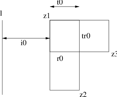
Thus in both the chains and , at some point we have to use an empty rectangle with and . But since the labelings in both and are increasing, and is the smallest value of that we can start with, we have to start with . Thus, this fixes .
Now, let us assume that . We need an induction statement to show that is fixed. For each coordinate of , consider the horizontal line segment lying on some curve, which starts at and ends at and goes right throughout. We call admissible if every point just below the line segment belongs to . Since the starting empty rectangles in the chains and have , there is at least one admissible coordinate. Among all the admissible coordinates, let be the one with having the smallest length. Let be the smallest length, measured by number of intersections with curves. Our induction claim states: in any maximal chain in , at some point we have to use an empty rectangle with and . The induction is done on the length of . Clearly when the length is , the claim is true. Let us assume that we start with an empty rectangle with and . Since has Maslov index one, so it cannot contain any coordinate in its interior, and it also cannot contain any horizontal annulus. Therefore, it is easy to see that has to be disjoint from , and thus has Maslov index one lower than and still intersects and has an admissible coordinate with . Thus induction applies, and proves our claim. It is obvious that the starting empty rectangles in the chains and must have and . Since both have increasing labelings, we must start with empty rectangles with .
Next, we want to show that is also fixed. This is also done by an induction very similar to the ones above. Consider all with , such that the covering relation has . Let be the thinnest empty rectangle among all such covering relations, and let be the thickness of . The induction claim states: in any maximal chain in , at some point we have to use an empty rectangle with and , and the induction is done on the length of . Once again, it is trivial when the length is . Assume that we start with a empty rectangle with and . The empty rectangles and must look like Figure 4.4.
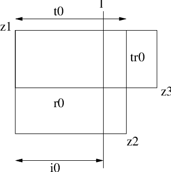
Note that has Maslov index one lower than and it still intersects , and it still has an admissible coordinate with . Thus induction applies. Since the labelings for and are both increasing, this implies that they both must start with an empty rectangle with . Thus we see that the thickness is fixed. As explained earlier, this finishes the proof. ∎
Proof of Theorem 4.1.
Fix a closed interval . By Lemma 4.3, there is at most one maximal chain in , namely the one whose labeling is lexicographically the minimum, for which the the labeling is increasing. Lemma 4.2 tells us that the lexicographically minimum labeling is also an increasing labeling. Therefore, there is a unique maximal chain in for which the labeling is increasing, and that labeling is lexicographically the minimum. ∎
5. Flow category
Inspired by the definition of the flow category in [CJS95], let us define a PL flow category to be a small category with the following additional structures and properties: there is a grading assignment ; for any , the set consists of only the identity; for any two distinct , the set is a (possibly empty) -dimensional PL-manifold (possibly with boundary); for any , the map is a PL-embedding, such that if are distinct, then the image of the embedding is a subspace of the boundary of ; furthermore, if is a point on the boundary, then there exists , such that is in the image of the embedding .
In this section, given a GT poset whose every closed interval is shellable, we will construct a PL flow category . There will also be a natural functor from to , the category associated to the poset .
The objects of are the elements of , and the grading assignment on is simply the grading assignment of . The space is non-empty if and only if . If , consider the interval ; let be its barycentric subdivision, and now consider the interval in ; the space is defined to be its order complex, . Let ; before we define the structure map , observe that the Cartesian product of the poset , viewed as an interval in , and the poset , viewed as an interval in , is naturally isomorphic to the poset , viewed as an interval in ; the structure map is the composition .
Theorem 5.1.
Proof.
Let . We will prove that is PL-homeomorphic to the -dimensional ball. Since the interval is graded with length , the interval in is graded with length . Since is locally thin, the interval is thin, and therefore, the interval in is subthin; furthermore, a submaximal chain of is covered by exactly one maximal chain if and only if it does not contain . Finally, since the interval is shellable, we know from Theorem 2.1 that the interval is shellable. Therefore, Theorem 2.3 applies and tells us that the order complex is PL-homeomorphic to the -dimensional ball; furthermore, the boundary of the ball corresponds precisely to the submaximal chains of that do not contain .
Now let . Next, we will prove that the map is a PL-embedding into the boundary of . The map is an embedding because it is essentially the inclusion of as a subcomplex of . Its image lies in the boundary of because none of the chains in contain the point .
Finally, let us prove that every point in the boundary of is in the image of such an embedding. Let be a point in the boundary. Let be a maximal dimensional simplex in the boundary of that contains . Let be the submaximal chain in that corresponds to . Since lies in the boundary, does not contain the element . Therefore, the smallest element of is some element of the form , with . Then lies in the image of the map . ∎
Therefore, using Lemma 3.6, Theorem 4.1 and Theorem 2.2, we can associate a PL flow category to a grid diagram in a natural way. This suggests that we might be able to associate a stable homotopy type to a grid diagram in a natural way, whose homology will be the knot Floer homology. However, in order to apply the Cohen-Jones-Segal machinery [CJS95], we need to frame the tangent bundles of in a coherent way: namely, for every , we want a trivialization of the bundle over , such that whenever , the trivialization of the bundle over induces the trivialization of the bundle over the image of the inclusion .
It is not clear what is the relevant notion of the tangent bundle of a PL-manifold. More importantly, it is not clear how to produce these coherent framings starting with a GT poset whose every closed interval is shellable. It seems likely that to do so we need more structures on the poset. It would be an interesting endeavor to characterize those extra structures, and to check if the GT posets arising from grid diagrams have them.
References
- [Bjö80] Anders Björner, Shellable and Cohen-Macaulay partially ordered sets, Transactions of the American Mathematical Society 260 (1980), no. 1, 159–183.
- [Bjö84] by same author, Posets, regular CW complexes and Bruhat order, European Journal of Combinatorics 5 (1984), no. 1, 7–16.
- [Bru98] H. Brunn, Über verknotete Kurven, Verhandlungen des Internationalen Math Kongresses (Zurich 1897) (1898), 256–259.
- [BW83] Anders Björner and Michelle Wachs, On lexicographically shellable posets, Transactions of the American Mathematical Society 277 (1983), no. 1, 323–341.
- [CJS95] Ralph Cohen, John Jones, and Graeme Segal, Floer’s infinite-dimensional Morse theory and homotopy theory, vol. Floer Memorial Volume, Progress in Mathematics, no. 133, Birkhäuser, 1995.
- [Cro95] Peter Cromwell, Embedding knots and links in an open book I: Basic properties, Topology and its Applications 64 (1995), no. 1, 37–58.
- [DK74] Gopal Danaraj and Victor Klee, Shellings of spheres and polytopes, Duke Mathematical Journal 41 (1974), no. 2, 443–451.
- [Lyo80] Herbert C. Lyon, Torus knots in the complement of links and surfaces, Michigan Math Journal 27 (1980), no. 1, 39–46.
- [Mat06] Hiroshi Matsuda, Links in an open book decomposition and in the standard contact structure, Proceedings of the American Mathematical Society 134 (2006), 3697–3702.
- [MOS09] Ciprian Manolescu, Peter Ozsváth, and Sucharit Sarkar, A combinatorial description of knot Floer homology, Annals of Mathematics 169 (2009), no. 2, 633–660.
- [MOSzT07] Ciprian Manolescu, Peter Ozsváth, Zoltán Szabó, and Dylan Thurston, On combinatorial link Floer homology, Geometry and Topology 11 (2007), 2339–2412.
- [Neu84] Lee Neuwirth, *-projections of knots, vol. Global Differential Geometry, Teubner-Texte zur Mathematik, no. 70, 1984.
- [Ni07] Yi Ni, Knot Floer homology detects fibred knots, Inventiones Mathematicae 170 (2007), no. 3, 577–608.
- [OSz03] Peter Ozsváth and Zoltán Szabó, Knot Floer homology and the four-ball genus, Geometry and Topology 7 (2003), 625–639.
- [OSz04a] by same author, Holomorphic disks and genus bounds, Geometry and Topology 8 (2004), 311–334.
- [OSz04b] by same author, Holomorphic disks and knot invariants, Advances in Mathematics 186 (2004), no. 1, 58–116.
- [OSz04c] by same author, Holomorphic disks and three-manifold invariants: properties and applications, Annals of Mathematics 159 (2004), no. 3, 1159–1245.
- [OSz04d] by same author, Holomorphic disks and topological invariants for closed three-manifolds, Annals of Mathematics 159 (2004), no. 3, 1027–1158.
- [OSz08a] by same author, Holomorphic disks, link invariants and the multi-variable Alexander polynomial, Algebraic and Geometric Topology 8 (2008), 615–692.
- [OSz08b] by same author, Link Floer homology and the Thurston norm, Journal of the American Mathematical Society 21 (2008), no. 3, 671–709.
- [Ras03] Jacob Rasmussen, Floer homology and knot complements, Ph.D. thesis, Harvard University, 2003.
- [Rud92] Lee Rudolph, Quasipositive annuli (constructions of quasipositive knots and links IV), Journal of Knot Theory and its Ramifications 4 (1992), 451–466.