Electroweak symmetry breaking at the LHC

In the SM there exists only one isodoublet complex scalar field and, thus, there are initially four real scalar fields [1, 2, 3, 4]. After spontaneous EWSB, we are left with one physical degree of freedom, the Higgs scalar and the other three would–be Nambu-Goldstone bosons are absorbed to build up the longitudinal components of the $W^{\pm},Z$ gauge bosons and generate their masses. Yukawa interactions of the fermions with the same scalar field give rise to the fermion masses. The Higgs scalar has ${\rm J^{\rm PC}=0^{++}}$ assignments of spin, parity and charge conjugation quantum numbers. The Higgs couplings to the fermions and gauge bosons are related to the masses of these particles and are thus decided by the symmetry breaking mechanism. In contrast, the mass of the Higgs boson itself is completely undetermined in the model. There are, however, both experimental and theoretical constraints on this fundamental parameter, which we will summarize below.

One available direct information on the Higgs mass is the lower limit $M_{H}\raisebox{-3.69899pt}{~\shortstack{$>$ \\ [-0.07cm] $\sim$}}~114.4$ GeV at 95% confidence level (c.l.) established at LEP2 [6]. The collaborations have also reported a small, $\raisebox{-3.69899pt}{~\shortstack{$<$ \\ [-0.07cm] $\sim$}}~2\sigma$, excess of events beyond the expected SM backgrounds, consistent with a SM–like Higgs boson with a mass $M_{H}\sim 115$ GeV [6]. In addition to this, the Tevatron physics potential for the discovery of Higgs particles looks promising, with the coming larger data sets. In particular, evidence for the SM Higgs boson could be obtained if the mass is near the observed experimental lower limit from LEP of about $115$ GeV or if it is near 160 GeV. In fact, with the run-II data collected by both the experiments, corresponding to $2.5$ fb^-1, the observed upper limits are a factor $3.7\,(1.1)$ higher than the expected SM Higgs cross section at $M_{H}=115\,(160)$ GeV at $95\%$ c.l. [7].

Furthermore, the high accuracy of the electroweak data measured at LEP, SLC and the Tevatron [8] provides an indirect sensitivity to $M_{H}$: the Higgs boson contributes logarithmically, $\propto\log(M_{H}/M_{W})$, to the radiative corrections to the $W/Z$ boson propagators. A recent analysis, which uses the updated determination of the top quark mass ($172.4$ GeV), yields the value $M_{H}=84^{+34}_{-26}$ GeV, corresponding to a 95% confidence level upper limit of $M_{H}\raisebox{-3.69899pt}{~\shortstack{$<$ \\ [-0.07cm] $\sim$}}~154$ GeV [5]. A very recent analysis, using a new fitting program gives the more precise value $M_{H}=116.4^{+18.3}_{-1.3}$ GeV [9].

Fig. 1 shows the global fit to the electroweak data and the ensuing limit on the Higgs mass. The limit increases to $185$ GeV when the LEP2 direct search limit of $114$ GeV is included. If the Higgs boson turns out to be significantly heavier than these upper limits, $M_{H}\raisebox{-3.69899pt}{~\shortstack{$>$ \\ [-0.07cm] $\sim$}}~200$ GeV, there should be an additional new ingredient that is relevant at the EWSB scale which the next round of experiments should reveal.

From the theoretical side, interesting constraints can be derived from assumptions on the energy range within which the SM is valid before perturbation theory breaks down and new phenomena would emerge. For instance, if the Higgs mass were larger than $\sim$ 1 TeV, the $W$ and $Z$ bosons would have to interact very strongly with each other so that their scattering at high energies respects unitarity. Imposing the unitarity requirement in the high–energy scattering of gauge bosons leads to the bound $M_{H}\raisebox{-3.69899pt}{~\shortstack{$<$ \\ [-0.07cm] $\sim$}}~700$ GeV [10]. If the Higgs boson were too heavy, unitarity would be violated in these processes at energies above $\sqrt{s}\raisebox{-3.69899pt}{~\shortstack{$>$ \\ [-0.07cm] $\sim$}}~1.2$ TeV and new phenomena should appear to restore it. It is interesting to note, as an aside, that just the requirement of perturbative unitarity in $WW$ scattering leads to a model with exactly the same particle content and couplings as the SM [11].

Another important theoretical constraint comes from the fact that the quartic Higgs self–coupling, which at the scale $M_{H}$ is fixed by $M_{H}$ itself, grows logarithmically with the energy scale. If $M_{H}$ is small, the energy cut–off $\Lambda$ at which the coupling grows beyond any bound and new phenomena should occur, is large; if $M_{H}$ is large, the cut–off $\Lambda$ is small. The condition $M_{H}\raisebox{-3.69899pt}{~\shortstack{$<$ \\ [-0.07cm] $\sim$}}~\Lambda$ sets an upper limit on the Higgs mass in the SM, the so called triviality bound. A naive one–loop analysis assuming the validity of perturbation theory [12] as well as lattice simulations [13] lead to the estimate $M_{H}\raisebox{-3.69899pt}{~\shortstack{$<$ \\ [-0.07cm] $\sim$}}~630$ GeV for this limit. Furthermore, loops involving top quarks tend to drive the coupling to negative values for which the vacuum is no longer stable.

Requiring the SM to be extended to, for instance, the GUT scale $\Lambda_{\rm GUT}\sim 10^{16}$ GeV and including the effect of top quark loops on the running coupling, the Higgs boson mass should lie in the range 130 GeV $\raisebox{-3.69899pt}{~\shortstack{$<$ \\ [-0.07cm] $\sim$}}~M_{H}\raisebox{-3.69899pt}{~\shortstack{$<$ \\ [-0.07cm] $\sim$}}~180$ GeV [14]; see Fig. 2. In fact, in any model beyond the SM in which the theory is required to be weakly interacting up to the GUT or Planck scales, the Higgs boson should be lighter than $M_{H}\raisebox{-3.69899pt}{~\shortstack{$<$ \\ [-0.07cm] $\sim$}}~200$ GeV. Such a Higgs particle can be thus produced at the LHC.

Once its mass is fixed the profile of the Higgs particle is uniquely determined and its production rates and decay widths are fixed. As its couplings to different particles are proportional to their masses, the Higgs boson will have the tendency to decay into the heaviest particles allowed by phase space. The Higgs decay modes and their branching ratios (BR) are briefly summarized below; see Ref. [15] for details.

In the “low–mass” range, $M_{H}\raisebox{-3.69899pt}{~\shortstack{$<$ \\ [-0.07cm] $\sim$}}~130$ GeV, the Higgs boson decays into a large variety of channels. The main mode is by far the decay into $b\bar{b}$ with BR $\sim$ 90% followed by the decays into $c\bar{c}$ and $\tau^{+}\tau^{-}$ with BRs $\sim$ 5%. Also of significance is the top–loop mediated decay into gluons, which occurs at the level of $\sim$ 5%. The top and $W$–loop mediated $\gamma\gamma$ and $Z\gamma$ decay modes, which lead to clear signals, are very rare with BRs of ${\cal O}(10^{-3})$.

In the “high–mass” range, $M_{H}\raisebox{-3.69899pt}{~\shortstack{$>$ \\ [-0.07cm] $\sim$}}~130$ GeV, the Higgs bosons decay into $WW$ and $ZZ$ pairs, one of the gauge bosons being possibly virtual below the thresholds. Above the $ZZ$ threshold, the BRs are 2/3 for $WW$ and 1/3 for $ZZ$ decays, and the opening of the $t\bar{t}$ channel for higher $M_{H}$ does not alter this pattern significantly.

In the low–mass range, the Higgs is very narrow, with $\Gamma_{H}<10$ MeV, but this width increases, reaching 1 GeV at the $ZZ$ threshold. For very large masses, the Higgs becomes obese, since $\Gamma_{H}\sim M_{H}$, and can hardly be considered as a resonance.

The branching ratios and total decay widths are summarized in Fig. 3, which is obtained from a recently updated version of the code HDECAY [16] and where the new value $m_{t}=172$ GeV is used as an input.

The SM in spite of its spectacular success, is ridden with two well known problems, which are the major stumbling blocks while trying to extend the validity of the SM to the GUT scale $\Lambda_{\rm GUT}$. The first one is the so–called naturalness problem: the radiative corrections to $M_{H}$ being quadratically divergent push the Higgs boson mass to be the order of these large scales. The second problem is that the running of the three gauge couplings of the SM is such that they do not meet at a single point and thus do not unify at the GUT scale.

Low energy supersymmetry solves these two problems at once [17]: supersymmetric particle loops cancel exactly the quadratic divergences and help stablise the Higgs boson mass at the weak scale, and they contribute to the running of the gauge couplings to allow their unification at $\Lambda_{\rm GUT}$. In addition, it allows for a good candidate for the dark matter in the universe.

The minimal supersymmetric extension of the SM (MSSM), requires the existence of two isodoublet Higgs fields to cancel anomalies and to give mass separately to up and down–type fermions. Two CP–even neutral Higgs bosons $h,H$, a pseudoscalar $A$ boson and a pair of charged scalar particles, $H^{\pm}$, are introduced by this extension of the Higgs sector [3, 17, 18]. In fact, in this case, the scalar potential does not involve an arbitrary self coupling $\lambda$ as is the case with the SM, but involves only the gauge couplings and as a result the mass of the lightest Higgs boson $h$ is bounded from above. Besides the four masses, the properties of the Higgs sector in the MSSM are determined by two more parameters : a mixing angle $\alpha$ in the neutral CP–even sector and the ratio of the two vacuum expectation values $\tan\beta$. The value of the latter lies in the range $1\raisebox{-3.69899pt}{~\shortstack{$<$ \\ [-0.07cm] $\sim$}}~\tan\beta\raisebox{-3.69899pt}{~\shortstack{$<$ \\ [-0.07cm] $\sim$}}~m_{t}/m_{b}$.

Supersymmetry leads to several relations among these parameters and only two of them, taken in general to be $M_{A}$ and $\tan\beta$, are in fact independent. These relations impose a strong hierarchical structure on the mass spectrum, $M_{h}\!<\!M_{Z},M_{A}\!<\!M_{H}$ and $M_{W}\!<\!M_{H^{\pm}}$, which however is broken by radiative corrections as the top quark mass is large; see Ref. [19] for a review. The leading part of this correction grows as the fourth power of $m_{t}$ and logarithmically with the SUSY scale or common squark mass $M_{S}$; the mixing (or trilinear coupling) in the stop sector $A_{t}$ plays an important role. For instance, the upper bound on the mass of the lightest Higgs boson $h$ is shifted from the tree level value $M_{Z}$ to $M_{h}\sim 130$–140 GeV in the maximal mixing scenario where $X_{t}=A_{t}-\mu/\tan\beta\sim 2M_{S}$ with $M_{S}={\cal O}(1$ TeV) [19]; see left panel of Fig. 4. The masses of the heavy neutral and charged Higgs particles are expected to range from $M_{Z}$ to the SUSY breaking scale $M_{S}$.

The pseudoscalar Higgs boson $A$ has no tree level couplings to gauge bosons, and its couplings to down (up) type fermions are (inversely) proportional to $\tan\beta$. This is also the case for the couplings of the charged Higgs boson to fermions, which are admixtures of scalar and pseudoscalar currents and depend only on $\tan\beta$. For the CP–even Higgs bosons $h$ and $H$, the couplings to down (up) type fermions are enhanced (suppressed) compared to the SM Higgs couplings for $\tan\beta>1$. They share the SM Higgs couplings to vector bosons as they are suppressed by $\sin$ and $\cos(\beta-\alpha)$ factors, respectively for $h$ and $H$. The Higgs couplings to the $W^{\pm},Z$ bosons are displayed in the right panel of Fig. 4.

If the pseudoscalar mass is large, the $h$ boson mass reaches its upper limit [which, depending on the value of $\tan\beta$ and stop mixing, is in the range 100–140 GeV] and its couplings to fermions and gauge bosons are SM–like; the heavier CP–even $H$ and charged $H^{\pm}$ bosons become degenerate with the pseudoscalar $A$ boson and have couplings to fermions and gauge bosons of the same intensity. In this decoupling limit, which can be already reached for masses $M_{A}\raisebox{-3.69899pt}{~\shortstack{$>$ \\ [-0.07cm] $\sim$}}~300$ GeV, it is very difficult to distinguish the Higgs sectors of the SM and MSSM if only the lighter $h$ particle is observed.

Finally we note the experimental constraints on the MSSM Higgs masses, coming mainly from the negative LEP2 searches [20]. In the decoupling limit where the $h$ boson is SM–like, the limit $M_{h}\raisebox{-3.69899pt}{~\shortstack{$>$ \\ [-0.07cm] $\sim$}}~114$ GeV from the Higgs–strahlung $e^{+}e^{-}\to hZ$ process holds; this constraint rules out $\tan\beta$ values smaller than $\tan\beta\sim 3$. Combining all processes, the current limits in the CP conserving MSSM at $95\%$ c.l., assuming no invisible decays, are [8, 20]: $M_{h}>92.4$ GeV, $M_{A}>93.4$ GeV for $\tan\beta>0.4$ and $M_{H^{\pm}}>79.3$ GeV. Fig. 5 shows the current limits from LEP and Tevatron data on the MSSM Higgs sector.

Let us now turn to the decays of the MSSM Higgs particles; Fig. 6. The lightest $h$ boson will decay mainly into fermion pairs since $M_{h}\raisebox{-3.69899pt}{~\shortstack{$<$ \\ [-0.07cm] $\sim$}}~$ 140 GeV. This is, in general, also the dominant decay mode of the $A$ and $H$ bosons, since for $\tan\beta\gg 1$, they decay into $b\bar{b}$ and $\tau^{+}\tau^{-}$ pairs with BRs of the order of $\sim$ 90% and 10%, respectively. For large masses, the top decay channels $H,A\rightarrow t\bar{t}$ open up, yet they are suppressed for large $\tan\beta$. The $H$ boson can decay into gauge bosons or $h$ boson pairs, and the $A$ particle into $hZ$ final states; however, these decays are strongly suppressed for $\tan\beta\raisebox{-3.69899pt}{~\shortstack{$>$ \\ [-0.07cm] $\sim$}}~5$. The $H^{\pm}$ particles decay into fermions pairs: mainly $t\bar{b}$ and $\tau\nu_{\tau}$ final states for $H^{\pm}$ masses, respectively, above and below the $tb$ threshold. If allowed kinematically, they can also decay into $hW$ final states for $\tan\beta\raisebox{-3.69899pt}{~\shortstack{$<$ \\ [-0.07cm] $\sim$}}~5$. Adding up the various decays, the widths of all five Higgses remain rather narrow; Fig. 7.

Other possible decay channels for the heavy $H,A$ and $H^{\pm}$ states, are decays into light charginos and neutralinos, which could be important if not dominant; decays of the $h$ boson into the invisible lightest neutralinos (LSP) can also be important, exceeding 50% in some parts of the parameter space and altering the searches at hadron colliders [21, 22]. Decays into (third generation) squarks and sleptons can also occur for the heavy Higgs states but are in general suppressed, in particular at high $\tan\beta$. See Ref. [18] for more details.

Note finally, that light SUSY particles can also affect the branching ratio of the loop–induced modes in a sizable way [23]. In particular, light stops can significantly affect the $h\to gg$ decay mode while light stops and charginos can alter the photonic Higgs decays [23, 21].

A quantitative explanation of baryogenesis requires physics beyond the SM, one possibility being an additional source of CP violation beyond the one present in the SM via CKM mixing. CP–violation in the SUSY sector is one such source which allows explanation of baryogenesis at the electroweak scale. A general two Higgs doublet model seems to be able to generate adequate amount of baryon asymmetry in the universe (BAU) and be consistent with the current experimental constraints such as electric dipole moments [24]. In the MSSM, it may be possible to satisfy all the low energy constraints and still have sufficient CP violation in the theory to explain the BAU quantitatively (without requiring too much fine-tuning, one needs to go to non-minimal versions [25]). This further causes new phases to enter the MSSM Higgs sector, which is CP–conserving at tree–level, through the large radiative corrections. These phases affect both the masses and the couplings of the neutral and charged Higgs particles, thus having very serious implications for the Higgs phenomenology at the LHC. This issue has received a lot of attention in the recent times [26, 27, 28, 29, 30].

Since CP is violated, the three mass eigenstates $H_{1},H_{2},H_{3}$ need no longer have definite CP quantum numbers and can be a mixture of the $h,H,A$ states. The subscript $i$ indicates the order of the mass $m_{H_{i}}$ of the $H_{i}$ boson in the spectrum, i.e. $m_{H_{1}}\!<\!m_{H_{2}}\!<\!m_{H_{3}}$. It is obvious that this will lead to significant modification of the properties of the various Higgs particles. Effect of this mixing on the couplings of the mixed CP states $H_{1},H_{2},H_{3}$ with a pair of gauge bosons/fermions i.e., $H_{i}f\bar{f}$, $H_{i}VV$, can change the Higgs phenomenology profoundly. For details, see e.g. Refs. [26, 27, 28, 29, 30].

In multi-Higgs doublet models, there exist sum rules which force the different $H_{i}$ bosons to share among themselves the coupling of the SM Higgs boson to the massive gauge bosons [31], $\sum_{i}g_{H_{i}VV}^{2}=g^{2}_{H_{\rm SM}}$. However, it is only the CP–even component that is projected out. A CP violating MSSM is distinguished from a general CP violating two-Higgs doublet model by the fact that the former has a prediction for the mixing in terms of SUSY-breaking CP-violating phases of the MSSM. The possible dilution of the LEP limits on the Higgs masses due to CP violation had been discussed in a model independent formulation [32]. The specific feature of the CP-violating MSSM is the prediction for the mixing in terms of the SUSY parameters and CP breaking phases that they have.

As examples of new features in the CP violating MSSM, compared to the usual MSSM, we simply mention the possibility of a relatively light $H_{1}$ state with very weak couplings to the gauge bosons, and which could have escaped detection at LEP2 [30, 33, 20] and the possibility of resonant $H/A$ mixing when the two Higgs particles are degenerate in mass [34]. An example of the Higgs mass spectrum in the so-called CPX scenario in which $H_{1}$ can be light is shown in Fig. 8 (left) as a function of the phase of the coupling $A_{t}$.

Fig. 8 (right) shows the result for the Higgs couplings to gauge bosons in the same CPX scenario for two different values of the gluino mass phase. In fact, the non observation of a Higgs boson signal in the direct searches at the LEP, reinterpreted in the MSSM with CP violation, shows [33, 20] that indeed there are holes in the excluded region at small $\tan\beta$ and $m_{H_{1}}$ in the $\tan\beta$–$M_{H_{1}}$ plane; see Fig. 9. This corresponds to the case of $H_{1}$ decoupled from the $Z$ boson, mentioned above.

Of course such features will have to be proved to be the result of CP–violation by, for instance, studying CP–odd observables and associated phenomenology.

The Higgs sector in SUSY models can be more complicated than previously discussed if some basic assumptions of the MSSM, such as the presence of only two Higgs doublet fields, or R–parity conservation, are relaxed. A few examples are listed below.

The next–to–minimal SUSY extension, the NMSSM, in which the spectrum of the MSSM is extended by one singlet superfield [35], was among the first SUSY models based on supergravity-induced SUSY-breaking terms. It has gained a renewed interest in the last decade, since it solves in a natural and elegant way the so-called $\mu$ problem [36] of the MSSM; in the NMSSM this parameter is linked to the vev of the singlet Higgs field, generating a $\mu$ value close to the SUSY-breaking scale. Furthermore, when the soft breaking terms are assumed to be universal at the GUT scale, the resulting constrained model (cNMSSM) is very constrained as one single parameter (e.g. the gaugino mass $M_{1/2}$) allows to fully describe its phenomenology [37].

The NMSSM leads to an interesting phenomenology [38, 39] as the MSSM spectrum is extended to include an additional CP-even and CP-odd Higgs states as well as a fifth neutralino, the singlino. An example of the Higgs mass spectrum in the cNMSSM [37] is shown in Fig. 10 as a function of the gaugino mass parameter. As in the MSSM in the decoupling regime, the heaviest CP-even, CP-odd and charged Higgs states form a practically degenerate SU(2) multiplet with a common mass beyond 500 GeV; the lightest CP-even state is mostly SM-like, with a mass increasing slightly with $M_{1/2}$ from 115 GeV up to $\sim 120$ GeV. The third CP-even state has a dominant singlet component: for small $M_{1/2}$ it is lighter than the SM-like Higgs boson, escaping LEP constraints due to the very small coupling to the $Z$ boson. For increasing values of $M_{1/2}$, its mass increases until it becomes comparable and eventually exceeds the mass of SM-like CP-even Higgs state.

However, in the unconstrained NMSSM, the effect of the additional singlet to the scalar potential leads to a relaxation of the upper bound on the mass of the lighter CP–even particle above that of the MSSM $h$ boson [40]. Further, the constraints in the $M_{A}$–$\tan\beta$ plane, implied by the negative results of the LEP2 searches are less restrictive as compared to those in the MSSM [26, 41]. In addition, there exists a small region not yet completely excluded, where the lightest CP–even Higgs boson might have escaped the LEP2 searches. Even more interestingly, there exist possibilities that one of the neutral Higgs particles, in particular the lightest pseudoscalar $A_{1}$, is very light with a mass of a few ten’s of GeV. The light CP–even Higgs, which is SM–like in general, could then decay into pairs of $A_{1}$ bosons, $H_{1}\to A_{1}A_{1}\to 4b,4\tau$, with a large branching fraction.

Higgs bosons in GUT theories. A large variety of theories, string theories, grand unified theories, left–right symmetric models, etc., suggest an additional gauge symmetry which may be broken only at the TeV scale. This leads to an extended particle spectrum and, in particular, to additional Higgs fields beyond the minimal set of the MSSM. Especially common are new U(1)’ symmetries broken by the vev of a singlet field (as in the NMSSM) which leads to the presence of a $Z^{\prime}$ boson and one additional CP–even Higgs particle compared to the MSSM; this is the case, for instance, in the exceptional MSSM [42] based on the string inspired $E_{6}$ symmetry. The secluded ${\rm SU(2)\times U(1)\times U(1)^{\prime}}$ model [43], in turn, includes four additional singlets that are charged under U(1)’, leading to 6 CP–even and 4 CP–odd neutral Higgs states. Other exotic Higgs sectors [26, 44] are, for instance, Higgs representations that transform as SU(2) triplets or bi–doublets under the ${\rm SU(2)_{L}}$ and ${\rm SU(2)_{R}}$ groups in left–right symmetric models, that are motivated by the seesaw approach to explain the small neutrino masses and which lead e.g. to a doubly charged Higgs boson $H^{--}$. These extensions, which also predict extra matter fields, would lead to a very interesting phenomenology and new collider signatures in the Higgs sector. We will not be discussing much about this subject in this review.

In a general SUSY model, with an arbitrary number of singlet and doublet scalar fields (as well as a matter content which allows for the unification of the gauge couplings), a linear combination of Higgs fields has to generate the $W/Z$ masses and thus, from the triviality argument discussed earlier, a Higgs particle should have a mass below 200 GeV and significant couplings to gauge bosons [45]. The upper bound on the mass of the lightest Higgs boson in this most general SUSY model is displayed in Fig. 11 as a function of $\tan\beta$.

R–parity violating models. Models in which R–parity is spontaneously broken [and where one needs to either enlarge the SM symmetry or the spectrum to include additional gauge singlets], allow for an explanation of the light neutrino data [46]. Since $\not\hskip-4.2679ptR_{p}$ entails the breaking of the total lepton number $L$, one of the CP–odd scalars, the Majoron $J$, remains massless being the Goldstone boson associated to $\not\hskip-4.2679ptL$. In these models, the neutral Higgs particles have also reduced couplings to the gauge bosons. More importantly, the CP–even Higgs particles can decay into pairs of invisible Majorons, $H_{i}\to JJ$, while the CP–odd particle can decay into a CP–even Higgs and a Majoron, $A_{i}\to H_{i}J$, and three Majorons, $A\to JJJ$ [46].

There are also many non supersymmetric extensions of the SM which might lead to a different Higgs phenomenology. In some cases, the Higgs sector would consist of one scalar doublet leading to a Higgs boson which would mimic the SM Higgs, but the new particles that are present in the models might alter some of its properties. In other cases, the Higgs sector is extended to contain additional scalar fields leading to the presence of new Higgs particles. Another possibility is a scenario with a composite and strongly interacting Higgs, or where no Higgs particle is present at all, leading to strong interactions of the $W/Z$ bosons. Below we give a non exhaustive list of various possible scenarios.

Scenarios with Higgs mixing. In warped extra–dimensional models [47] the fluctuations of the size of the extra dimension about its stabilized value manifest themselves as a single scalar field, the radion. In the Randall Sundrum model with a bulk scalar field, it is expected that the radion is the lightest state beyond the SM fields with a mass probably in the range between ${\cal O}$(10 GeV) and $\Lambda={\cal O}$(TeV) [48, 49, 50]. The couplings of the radion are order of $1/\Lambda$ and are very similar to the couplings of the SM Higgs boson, except for one important difference: due to the trace anomaly, the radion directly couples to massless gauge bosons at one loop. Moreover, in the low energy four–dimensional effective theory, the radion can mix with the Higgs boson. This mixing can lead to important shifts in the Higgs couplings which become apparent in the Higgs decay widths and production cross sections; Fig. 12.

Another important consequence of radion mixing is the decays of the Higgs boson into a pair of radions. Indeed, if the radion is relatively light, the decays $H\to\phi\phi$ might be kinematically accessible and, for some mixing values, the branching fractions might be substantial. This is exemplified in Fig. 13 where BR($H\to\phi\phi$) is displayed in a specific scenario.

In large extra dimension models [51], mixing of the Higgs boson with graviscalars also occurs [52], leading to an invisible decay width. Mixing effects also occur if the SM is minimally extended in a renormalizable way to contain a singlet scalar field $S$ that does not couple to the other SM particles; its main effect would be to alter the scalar potential and to mix with the SM Higgs field [53] and, in such a case, the Higgs could mainly decay into two invisible $S$ particles.

Scenarios with extended Higgs/gauge/matter. Non–supersymmetric extensions of the Higgs sector with additional singlet, doublet and higher representation fields have also been advocated [44]. Examples are the minimal SM extension with a singlet discussed above, two–Higgs doublet models which potentially include CP–violation, triplet Higgs fields in models for light neutrino mass generation, etc… These extensions lead to a rich spectrum of Higgs particles which could be produced at the LHC. In other extensions of the SM, new gauge bosons and new matter particles are predicted and they can affect the properties of the SM–like Higgs boson. For instance the new fermions present in little Higgs and extra–dimensional models might contribute to the loop induced Higgs couplings, while new heavy gauge bosons could alter the Higgs couplings to $W$ and $Z$ bosons for instance. The anomalous $ZZH$ and $t\bar{t}H$ couplings can be a good probe of the additional scalars and/or the novel features of the geometry in the extra dimensions [54].

Scenarios with a composite Higgs boson. In little Higgs models [55], the dynamical scale is around $\Lambda=10$ TeV, unlike the traditional Technicolor model [56]. A light Higgs boson can be generated as a pseudo Goldstone boson and its mass of order 100 GeV is protected against large radiative corrections individually in the boson and the fermion sectors. The models predict a rich spectrum of new particles not only at the scale $\Lambda$ but also at lower scales. Axion–type pseudoscalar bosons may be associated with the spontaneous breaking of U(1) factors in the extra global symmetries [57]. These particles have properties analogous to Higgs bosons and can be produced at the LHC; deviations in the production and decay rates of the SM–like Higgs boson can also be induced by these particles. Note that, recently, a model–independent description of a strongly interacting light Higgs has been given [58].

Higgsless models and strong $W/Z$ interactions. Assuming the $W/Z$ bosons to become strongly interacting at TeV energies, damping the rise of the elastic $W/Z$ scattering amplitudes, is an alternative way to solve the problem of unitarity violation at high energies in the SM, without adding a relatively light Higgs boson. Naturally, the strong forces between the massive gauge bosons may be traced back to new fundamental interactions characterized by a scale of order 1 TeV [56]. Also in theories with extra space dimensions, EWSB can occur without introducing additional fundamental scalar fields, leading also to Higgsless theories [59]. Studying such difficult scenarios at the LHC will be possible with very high luminosity [60].

There are essentially four mechanisms for the single production of the SM Higgs boson at hadron colliders [61]; some Feynman diagrams are shown in Fig. 14.

The total cross sections, obtained with the programs of Ref. [62], are displayed in Fig. 15 for the LHC with $\sqrt{s}=14$ TeV as a function of the Higgs mass; the top quark mass is set to $m_{t}=178$ GeV and the MRST parton distributions functions [63] have been adopted. The NLO, and eventually NNLO, corrections have been implemented as will be summarized below, where we discuss the main features of each production channel.

a) $gg\to H$: This is by far the dominant production process at the LHC, up to masses $M_{H}\approx 1$ TeV. The most promising detection channels are [64] $H\to\gamma\gamma$ for $M_{H}\raisebox{-3.69899pt}{~\shortstack{$<$ \\ [-0.07cm] $\sim$}}~130$ GeV and slightly above this mass value, $H\to ZZ^{*}\to 4\ell^{\pm}$ and $H\to WW^{(*)}\to\ell\ell\nu\nu$ with $\ell=e,\mu$ for masses below, respectively, $2M_{W}$ and $2M_{Z}$. For higher Higgs masses, $M_{H}\raisebox{-3.69899pt}{~\shortstack{$>$ \\ [-0.07cm] $\sim$}}~2M_{Z}$, it is the golden mode $H\rightarrow ZZ\rightarrow 4\ell^{\pm}$, which from $M_{H}\raisebox{-3.69899pt}{~\shortstack{$>$ \\ [-0.07cm] $\sim$}}~500$ GeV can be complemented by $H\to ZZ\to\nu\bar{\nu}\ell^{+}\ell^{-}$ and $H\to WW\to\nu\ell jj$ to increase the statistics [65, 66, 67, 68, 69, 70].

The next–to–leading order (NLO) QCD corrections have been calculated in both the limit where the internal top quark has been integrated out [71], an approximation which should be valid in the Higgs mass range $M_{H}\raisebox{-3.69899pt}{~\shortstack{$<$ \\ [-0.07cm] $\sim$}}~300$ GeV, and in the case where the full quark mass dependence has been taken into account [72]. The corrections lead to an increase of the cross sections by a factor of $\sim 1.7$. The “tour de force” of deriving the three–loop corrections has been preformed in the infinite top–quark mass limit; these NNLO corrections lead to the increase of the rate by an additional 30% [73] (see also Refs. [74, 75]. This results in a nice convergence of the perturbative series and a strong reduction of the scale uncertainty, which is the measure of unknown higher order effects; see Fig. 16. The resummation of the soft and collinear corrections, performed at next–to–next–to–leading logarithm accuracy, leads to another increase of the rate by $\sim 5\%$ and a decrease of the scale uncertainty [76]. The QCD corrections to the differential distributions, and in particular to the Higgs transverse momentum and rapidity distributions, have also been recently calculated at NLO [with a resummation for the former] and shown to be rather large [77]. The dominant components of the electroweak corrections, some of which have been derived very recently, are comparatively very small [78].

b) $q\bar{q}\to HV$: The associated production with gauge bosons, with $H\to b\bar{b}$ and possibly $H\to WW^{*}\to\ell^{+}\nu jj$, is the most relevant mechanism at the Tevatron [7] [$gg\to H\to WW\to\ell\nu\ell\nu$ being important for Higgs masses close to 160 GeV]. At the LHC, this process plays only a marginal role; however, the channels $HW\to\ell\nu\gamma\gamma$ and eventually $\ell\nu b\bar{b}$ could be useful for the measurement of Higgs couplings.

The QCD corrections, which at NLO [79, 80], can be inferred from Drell–Yan production, have been calculated at NNLO [81]; they are $\sim$ 30% in total; see Fig. 17. The ${\cal O}(\alpha)$ electroweak corrections have been also derived recently [82] and decrease the rate by $5$ to 10%. The remaining scale dependence is very small, making this process the theoretically cleanest of all Higgs production processes.

c) The $WW/ZZ$ fusion mechanism: This process has the second largest cross section at the LHC. The QCD corrections, which can be obtained in the structure–function approach, are at the level of 10% and thus small [80, 83] (the electroweak corrections [84] are at the level of a few percent). The corrections including cuts, and in particular corrections to the $p_{T}$ and $\eta$ distributions, have also been calculated and implemented into a parton–level Monte–Carlo program [85]. With the specific cuts to the process, the output for the production cross section is shown in Fig. 18 for a Higgs in the mass range 100–200 GeV.

For several reasons, the interest in this process has grown in recent years: it has a large enough cross section [a few picobarns for $M_{H}\raisebox{-3.69899pt}{~\shortstack{$<$ \\ [-0.07cm] $\sim$}}~250$ GeV] and one can use cuts, forward–jet tagging, mini–jet veto for low luminosity as well as triggering on the central Higgs decay products] [86], which render the backgrounds comparable to the signal, therefore allowing precision measurements. In the past, it has been shown that the decay $H\to\tau^{+}\tau^{-}$ and possibly $H\to\gamma\gamma,ZZ^{*}$ can be detected and could allow for coupling measurements [68, 87, 88]. In the last years, parton–level analyzes have shown that various other channels can be possibly detected [89, 90]: $H\to WW^{*}$ for $M_{H}\sim$ 125–180 GeV, $H\to\mu^{+}\mu^{-}$ [for second–generation coupling measurements], $H\to b\bar{b}$ [for the $b\bar{b}H$ Yukawa coupling] and $H\to$ invisible (see later). Recent experimental simulations [67] have assessed more firmly the potential of this channel.

d) $pp\to t\bar{t}H$: Finally, Higgs boson production in association with top quarks, with $H\to\gamma\gamma$ or $b\bar{b}$, can in principle be observed at the LHC and direct measurement of the top Yukawa coupling, as well as an unambiguous determination of the CP of the Higgs can be possible. (Recent analyses have however, shown that $pp\to t\bar{t}H\to t\bar{t}b\bar{b}$ might be subject to a too large jet background [66]). The cross section is rather involved at tree–level since it is a three–body process, and the calculation of the NLO corrections was a real challenge which was met a few years ago [91]. The $K$–factors turned out to be rather small, $K\sim 1.2$ at the LHC. However, the scale dependence is drastically reduced from a factor two at LO to the level of 10–20% at NLO; see Fig.19. Note that the NLO corrections to the $q\bar{q}/gg\to b\bar{b}H$ process, which is more relevant in the MSSM, have been also completed [92]: compared with the NLO rate for the $bg\to bH$ process where the initial $b$-quark is treated as a parton [93, 94], the calculations agree within the scale uncertainties [95]. A similar situation occur for $H^{\pm}$ production in the $gb$ process: the $K$–factor is moderate $\sim\!1.2$–1.5 if the cross section is evaluated at scales $\mu\sim\frac{1}{2}(m_{t}+M_{H^{\pm}})$ [94].

Note that the PDF uncertainties have also been estimated for the four production processes: at the LHC, the uncertainties range from 5% to 15% depending on the considered process and the Higgs mass [96].

All the various channels discussed above have been discussed in great detail over the past decades [65, 66, 67, 68, 69, 70]. The significance for detecting the SM Higgs particle in the various production and decay channels is shown in Fig. 20, assuming a 100 fb^-1 integrated luminosity.

In the CP conserving MSSM, the production processes for the CP–even $h,H$ bosons are practically the same as for the SM Higgs and the ones depicted in Fig. 14 are all relevant. However, the $b$ quark will play an important role for moderate to large $\tan\beta$ values as its Higgs couplings are enhanced. First, one has to take into account the $b$ loop contribution in the $gg\to h,H$ process which becomes the dominant component in the MSSM [here, the QCD corrections are available only at NLO where they have been calculated in the full massive case [72] and increase the rate by $\sim 1.5$; SUSY-QCD corrections are discussed in Refs. [97, 98] e.g.]. Moreover, in associated Higgs production with heavy quarks, $b\bar{b}$ final states must be considered, $pp\to b\bar{b}+h/H$, and this process for either $h$ or $H$ becomes the dominant one in the MSSM [here, the QCD corrections are available in both the $gg$ and $gb\to b\Phi,b\bar{b}\to\Phi$ pictures [92, 93, 94, 95] depending on how many $b$–quarks are to be tagged, and which are equivalent if the renormalization and factorization scales are chosen to be small, $\mu\sim\frac{1}{4}M_{\Phi}$]. The rates for associated production with $t\bar{t}$ and $W/Z$ pairs as well as for $WW/ZZ$ fusion processes, are suppressed for at least one of the particles as a result of coupling reduction.

Because of CP invariance which forbids $AVV$ couplings, the $A$ boson cannot be produced in the Higgs-strahlung and vector boson fusion processes; the rate for the $pp\to t\bar{t}A$ process is suppressed by the small $At\bar{t}$ couplings for $\tan\beta\raisebox{-3.69899pt}{~\shortstack{$>$ \\ [-0.07cm] $\sim$}}~3$. Hence, only the $gg\to A$ fusion with the $b$–quark loops included [where the QCD corrections are also available only at NLO and are approximately the same as for the CP–even Higgs boson with enhanced $b$–quark couplings] and associated production with $b\bar{b}$ pairs, $pp\to b\bar{b}+A$ [where the QCD corrections are the same as for one of the CP–even Higgs bosons as a result of chiral symmetry] provide large cross sections. The one–loop induced processes $gg\to AZ,gg\to Ag$ [which hold also for one of the CP–even Higgses] and associated production with other Higgs particles, $pp\to A+h/H/H^{+}$ are possible but the rates are much smaller in general, in particular for $M_{A}\raisebox{-3.69899pt}{~\shortstack{$>$ \\ [-0.07cm] $\sim$}}~200$ GeV [99].

For the charged Higgs boson, the dominant channel is the production from top quark decays, $t\to H^{+}b$, for masses not too close to $M_{H^{\pm}}=m_{t}\!-\!m_{b}$; this is particularly true at low or large $\tan\beta$ when the $t\to H^{+}b$ branching ratio is significant. For higher masses [100], the processes to be considered is the fusion process $gg\to H^{\pm}tb$ supplemented by $gb\to H^{\pm}t$. The two processes have to be properly combined and the NLO corrections for both processes have been derived [94] and are moderate, increasing the cross sections by 20 to 50% if they are evaluated at low scales, $\mu\sim\frac{1}{2}(m_{t}+M_{H^{\pm}})$. Additional sources [101] of $H^{\pm}$ states for masses below $M_{H^{\pm}}\approx 250$ GeV are provided by pair and associated production with neutral Higgs bosons in $q\bar{q}$ annihilation as well as $H^{+}H^{-}$ pair and associated $H^{\pm}W^{\mp}$ production in $gg$ and/or $b\bar{b}$ fusion but the cross sections are not as large, in particular for $M_{H^{\pm}}\raisebox{-3.69899pt}{~\shortstack{$>$ \\ [-0.07cm] $\sim$}}~m_{t}$.

The cross sections for the dominant production mechanisms are shown in Fig. 21. as a function of the Higgs masses for $\tan\beta=3$ and $30$ for the same set of input parameters as used for the widths and branching ratios. The NLO QCD corrections are included, except for the $pp\to Q\bar{Q}\,$Higgs processes where, however, the scales have been chosen as to approach the NLO results; the MRST NLO structure functions have been adopted. As can be seen, at high $\tan\beta$, the largest cross sections are by far those of the $gg\to\Phi_{A}/A$ and $q\bar{q}/gg\to b\bar{b}+\Phi_{A}/A$ processes, where $\Phi_{A}=H\,(h)$ in the (anti–)decoupling regimes $M_{A}>(<)M_{h}^{\rm max}$: the other processes involving these two Higgs bosons have cross sections that are several orders of magnitude smaller. The production cross sections for the other CP–even Higgs boson, that is $\Phi_{H}=h\,(H)$ in the (anti–)decoupling regime when $M_{\Phi_{H}}\simeq M_{h}^{\rm max}$, are similar to those of the SM Higgs boson with the same mass and are substantial in all the channels which have been displayed. At small $\tan\beta$, the $gg$ fusion and $b\bar{b}$–Higgs cross sections are not strongly enhanced as before and all production channels, except for $b\bar{b}$–Higgs which is only slightly enhanced, have cross sections that are smaller than in the SM Higgs case, except for $h$ in the decoupling regime.

The principal detection signals of the neutral Higgs bosons at the LHC, in the various regimes of the MSSM, are as follows [18, 65, 66, 67, 68, 102].

a) Decoupling regime: One of the most interesting region is the decoupling regime, i.e. when $M_{h}\simeq M_{h}^{\rm max}$, the lighter $h$ boson is SM–like and has a mass smaller than $\approx 140$ GeV. It can be detected in the $h\to\gamma\gamma$ decays [possibly supplemented with a lepton in associated $Wh$ and $t\bar{t}h$ production], and eventually in $h\to ZZ^{*},WW^{*}$ decays in the upper mass range, and if the vector boson fusion processes are used, also in the decays $h\to\tau^{+}\tau^{-}$ and eventually $h\to WW^{*}$ in the higher mass range $M_{h}\raisebox{-3.69899pt}{~\shortstack{$>$ \\ [-0.07cm] $\sim$}}~130$ GeV; see Fig. 22. For relatively large values of $\tan\beta$ $(\tan\beta\raisebox{-3.69899pt}{~\shortstack{$>$ \\ [-0.07cm] $\sim$}}~10)$, the heavier CP–even $H$ boson which has enhanced couplings to down–type fermions, as well as the pseudoscalar Higgs particle, can be observed in the process $pp\to b\bar{b}+H/A$ where at least one $b$–jet is tagged and with the Higgs boson decaying into $\tau^{+}\tau^{-}$, and eventually, $\mu^{+}\mu^{-}$ pairs in the low mass range. With a luminosity of 30 fb^-1 (and in some cases lower) a large part of the $[\tan\beta,M_{A}]$ space can be covered as can be seen from Fig. 23.

b) Anti-decoupling regime: In the anti-decoupling regime, i.e. when $M_{A}<M_{h}^{\rm max}$ and at high $\tan\beta$ ($\raisebox{-3.69899pt}{~\shortstack{$>$ \\ [-0.07cm] $\sim$}}~10$), it is the heavier $H$ boson which will be SM–like and can be detected as above, while the $h$ boson will behave like the pseudoscalar Higgs particle and can be observed in $pp\to b\bar{b}+h$ with $h\to\tau^{+}\tau^{-}$ or $\mu^{+}\mu^{-}$ provided its mass is not too close to $M_{Z}$ not to be swamped by the background from $Z$ production. The part of the $[\tan\beta,M_{A}]$ space which can be covered is also shown in Fig. 23 and corresponds to $M_{A}\raisebox{-3.69899pt}{~\shortstack{$<$ \\ [-0.07cm] $\sim$}}~130$ GeV.

c) Intermediate coupling regime: In the intermediate coupling region, that is for not too large $M_{A}$ values and moderate $\tan\beta\raisebox{-3.69899pt}{~\shortstack{$<$ \\ [-0.07cm] $\sim$}}~5$, the interesting decays $H\rightarrow hh$, $A\rightarrow hZ$ and even $H/A\rightarrow t\bar{t}$ [as well as the decays $H^{\pm}\to Wh$] still have sizable branching fractions and can be searched for. In particular, the $gg\to H\to hh\to b\bar{b}\gamma\gamma$ process (the $4b$ channel is more difficult as a result of the large background) is observable for $\tan\beta\raisebox{-3.69899pt}{~\shortstack{$<$ \\ [-0.07cm] $\sim$}}~3$ and $M_{A}\raisebox{-3.69899pt}{~\shortstack{$<$ \\ [-0.07cm] $\sim$}}~300$ GeV, and would allow to measure the trilinear $Hhh$ coupling. These regions of parameter space may need to be reconsidered in the light of the new Tevatron value for the top mass.

d) Intense–coupling regime: In the intense–coupling region, that is for $M_{A}\sim M_{h}^{\rm max}$ and $\tan\beta\gg 1$, the three neutral Higgs bosons $\Phi=h,H,A$ have comparable masses and couple strongly to isospin $-\frac{1}{2}$ fermions leading to dominant decays into $b\bar{b}$ and $\tau\tau$ and large total decay widths [103, 102]. The three Higgs bosons can only be produced in the channels $gg\to\Phi$ and $gg/q\bar{q}\to b\bar{b}+\Phi$ with $\Phi\to b\bar{b},\tau^{+}\tau^{-}$ as the interesting $\gamma\gamma,ZZ^{*}$ and $WW^{*}$ decays of the CP–even Higgses are suppressed. Because of background and resolution problems, it is very difficult to resolve between the three particles. A solution advocated in Ref. [102] (see also Ref. [104]), would be to search in the channel $gg/q\bar{q}\to b\bar{b}+\Phi$ with the subsequent decay $\Phi\to\mu^{+}\mu^{-}$ which has a small BR, $\sim 3\times 10^{-4}$, but for which the better muon resolution, $\sim 1\%$, would allow to disentangle between at least two Higgs particles. The backgrounds are much larger for the $gg\to\Phi\to\mu^{+}\mu^{-}$ signals. The simultaneous discovery of the three Higgs particles is very difficult and in many cases impossible, as exemplified in Fig. 24 where one observes only one single peak corresponding to $h$ and $A$ production.

Finally, as mentioned previously, light $H^{\pm}$ particles with masses below $M_{H^{\pm}}\sim m_{t}$ can be observed in the decays $t\rightarrow H^{+}b$ with $H^{-}\rightarrow\tau\nu_{\tau}$; see Fig. 25. Heavier $H^{\pm}$ states can be probed for large enough $\tan\beta$, by considering the properly combined $gb\to tH^{-}$ and $gg\rightarrow t\bar{b}H^{-}$ processes using the decay $H^{-}\rightarrow\tau\nu_{\tau}$ and taking advantage of the $\tau$ polarization to suppress the backgrounds, and eventually the decay $H^{-}\to\bar{t}b$ which however, seems more problematic as a result of the large QCD background. See Ref. [105] for more detailed discussions on $H^{\pm}$ production and search strategies at the LHC.

The previous discussion on MSSM Higgs production and detection at the LHC might be significantly altered if some sparticles are relatively light. Some standard production processes can be affected, new processes can occur and additional channels involving SUSY final states might drastically change the Higgs detection strategies. Let us comment on some possibilities.

The $Hgg$ and $hgg$ vertices in the MSSM are mediated not only by heavy $t/b$ loops but also by loops involving squarks. If the top and bottom squarks are relatively light, the cross section for the dominant production mechanism of the lighter $h$ boson in the decoupling regime, $gg\to h$, can be significantly altered by their contributions. In addition, in the $h\to\gamma\gamma$ decay which is one of the most promising detection channels, the same $\tilde{t},\tilde{b}$ loops together with chargino loops, will affect the branching rate. The cross section times branching ratio $\sigma(gg\rightarrow h)\times{\rm BR}(h\rightarrow\gamma\gamma)$ for the lighter $h$ boson at the LHC can be thus very different from the SM, even in the decoupling limit in which the $h$ boson is supposed to be SM–like [23]. The effects can be drastic and could lead to a strong suppression of $\sigma(gg\rightarrow h\rightarrow\gamma\gamma)$.

If one of the top squarks is light and its coupling to the $h$ boson is enhanced, an additional process might provide a new source for Higgs particles in the MSSM: associated production with $\tilde{t}_{1}$ states, $pp\rightarrow gg/q\bar{q}\rightarrow\tilde{t}_{1}\tilde{t}_{1}h$ [106]. This is similar to the standard $pp\to t\bar{t}h$ mechanism and in fact, for small masses and large mixing of the $\tilde{t}_{1}$ the cross section can be comparable. Final states with the heavier $H,A,H^{\pm}$ and/or other squark species than $\tilde{t}_{1}$ are less favored by phase space.

Another possible source of MSSM Higgs bosons would be from the cascade decays of strongly interacting sparticles, which have large production rates at the LHC. In particular, the lighter $h$ boson and the heavier $A,H$ and $H^{\pm}$ particles with masses $\raisebox{-3.69899pt}{~\shortstack{$<$ \\ [-0.07cm] $\sim$}}~200$–300 GeV, can be produced from the decays of squarks and gluinos into the heavier charginos/neutralinos, which then decay into the lighter ones and Higgs bosons. This can occur either in “little cascades”, $\chi_{2}^{0},\chi_{1}^{\pm}\to\chi_{1}^{0}+\,$Higgs, or in “big cascades” $\chi_{3,4}^{0},\chi_{2}^{\pm}\to\chi_{1,2}^{0},\chi_{1}^{\pm}+\,$Higgs. The rates for ino decays into Higgs bosons can be dominant while decays of squarks/gluinos into the heavier inos are substantial. Detailed studies [107] have shown that these processes can be isolated in some areas of the SUSY parameter space and can be complementary to the direct production ones; see Fig. 26. In particular, one can probe the region $M_{A}\!\sim\!150$ GeV and $\tan\beta\!\sim\!5$, where only $h$ can be observed in standard searches.

The possibility of light charginos and neutralinos allows to search for the heavier $H,A$ and $H^{\pm}$ states in regions of the parameter space in which they are not accessible in the standard channels [this is the case e.g. for $M_{A}\sim 200$ GeV and moderate $\tan\beta$ values]. There are situations in which the signals for Higgs decays into charginos and neutralinos are clean enough to be detected at the LHC. One of the possibilities is that the neutral $H/A$ bosons decay into pairs of the second lightest neutralinos, $H/A\to\chi_{2}^{0}\chi_{2}^{0}$, with the subsequent decays of the latter into the LSP neutralinos and leptons, $\chi_{2}^{0}\to\tilde{\ell}^{*}\ell\to\chi_{1}^{0}\ell\ell$ with $\ell^{\pm}=e^{\pm},\mu^{\pm}$, through the exchange of relatively light sleptons. This leads to four charged leptons and missing energy in the final state. If the $H/A$ bosons are produced in the $gg$–fusion processes, there will be little hadronic activity and the $4\ell^{\pm}$ final state is clean enough to be detected. Preliminary analyzes show that the decays can be isolated from the large (SUSY) background; Fig. 27.

There are two ways by which CP violation in the MSSM affects the Higgs production rates and detection at the LHC, through mixing in the Higgs states and/or modification of loop induced $ggH_{i}$ and $\gamma\gamma H_{i}$ couplings due to CP violation in the squark couplings [26, 27, 28, 29, 30, 108, 109, 110, 111]. Ref. [108], for example, discusses the situation with no significant mixing between the $h,H$ and $A$ states and large effect on the $ggH_{1}$ coupling of CP violation in the squark-squark-Higgs vertex.

In Fig. 28, the contours of ratios of $h,H$ production rates in the CP violating MSSM to those without CP violation are shown. This corresponds to the case where the CP violation in the MSSM induces CPV $\tilde{q}\tilde{q}h(H)$ couplings. As expected from the sum rule we find that whereas the $h$ production rate increase in the allowed region, the $H$ production rate decreases. As can be seen from the Fig. 28 the effects can be considerable.

A more interesting aspect of CP violation in the Higgs sector is the vanishing of the coupling of the lightest Higgs scalar $H_{1}$ to the $Z$ pair mentioned earlier, which in fact invalidates the lower limit on the mass of the lightest neutral at the LHC. Further, due to the reduced $ggH_{1}$ and $t\bar{t}H_{1}$ couplings in this case, one may miss this state at the LHC too. The region of the parameter space where this happens, generically seems to correspond to the case where all the three neutral scalars and the charged scalar are reasonably light. This region of Ref. [29] corresponds to $\tan\beta\sim 3.5-5,M_{H^{+}}\sim 125-140$ GeV,  $M_{H_{1}}\stackrel{{\scriptstyle<}}{{{}_{\sim}}}50$ GeV and $\tan\beta\sim 2-3,M_{H^{+}}\sim 105-130~{\rm GeV},M_{H_{1}}\stackrel{{\scriptstyle<}}{{{}_{\sim}}}40$ GeV, for $\Phi_{CP}=90^{\circ}$ and $60^{\circ}$ respectively. (The details of the exact excluded region depend on the code used to compute the spectrum [112]). An analysis taking into account simulation of detector effects  [113] confirms that there exists a region in the $\tan\beta-M_{H^{+}}$ plane corresponding to $M_{H_{1}}<50$ GeV, $100<M_{H_{2}}<110$ GeV and $130<M_{H_{3}}<180$ GeV [29], where LHC does not seem to have reach.

This is shown in Fig. 29. In fact, the sum rules that the $H_{i}$ couplings must satisfy, come to the rescue [111] in recovering the lost Higgs signal. This is a very generic example of how one can ’recover’ the Higgs signal if the model parameters should contrive to make the usually investigated search channels ineffective. $H_{i}VV$ and $H_{i}H^{+}W$ couplings satisfy a sum rule given by: $g^{2}_{H_{i}VV}+|g_{H_{i}H^{+}W}|^{2}=1$. Further, there exists in the MSSM a correlation between the mass of the charged Higgs $M_{H^{\pm}}$ and that of the pseudo-scalar state. A suppressed $H_{1}VV$ coupling implies a light pseudo-scalar state, which in turn implies a light charged Higgs, with $M_{H^{+}}<M_{t}$. Hence, a light $H_{1}$ which might have been missed at LEP also corresponds to an $H^{\pm}$ light enough to be produced in $t$ decay, which in turn decays to $H_{1}W^{\pm}$, followed by $H_{1}$ decay to $b\bar{b}$. Due to the large $H^{\pm}\rightarrow H_{1}W^{\pm}$ branching ratio, the expected event rate for this final state is quite healthy ($\sim{\cal O}100$ fb), over the entire hole region; see Fig. 30.

Thus one can look for the $H_{1}$ in final states containing $bW^{+}bb\bar{b}W^{-}$ in the $t\bar{t}$ sample. The huge background ($\sim 8.5$ pb) coming from QCD production of $t\bar{t}\bar{b}b$, can be reduced to $\sim 0.5$ fb level and below, by demanding that one of the $bW$ combination reconstructs to $t$ mass and the $bbbW$ also to the $t$ mass [111, 69].

Fig. 31 shows the clustering of the $b\bar{b},b\bar{b}W$ and $b\bar{b}bW$ for the signal which can be used effectively to handle the background. These studies have thus opened up a new topology in which one should be looking for the lightest neutral Higgs in the decay of $H^{\pm}$ produced in $t$ decay. A few points are worth noticing. Due to the rather small value of $\tan\beta$ the usual $\tau\nu_{\tau}$ decay mode for the $H^{+}$ is also not available for the $H^{+}$ search in this case. Thus in this region of the MSSM parameter space, the above process provides a search prospect not just for the light neutral state which might have been missed at LEP, but also the light charged Higgs $H^{+}$ in this parameter range (a similar situation attains in NMSSM as well [114]). A theorists analysis [115] indicates that it may be possible to look at $\tilde{t}\bar{\tilde{t}}H_{1}$ production, which will be higher than in the corresponding CP conserving scenario due to lighter $H_{1}$, and have a signal for parameter values corresponding to the hole.

In the NMSSM, where a complex iso-scalar field is introduced, leading to an additional pair of scalar and pseudoscalar Higgs particles, the axion–type or singlino character of the pseudoscalar $A_{1}$ boson makes it preferentially light and decaying into $b$ quarks or $\tau$ leptons [26, 39, 69]. Therefore, in some areas of the NMSSM parameter space, the lightest CP–even Higgs boson may dominantly decay into a pair of light pseudoscalar $A_{1}$ bosons generating four $b$ quarks or $\tau$ leptons in the final state, $H_{1}\to A_{1}A_{1}\to 4b,2b2\tau,4\tau$. In fact, it is also possible that $H_{1}$ is very light with small $VV$ couplings, while $H_{2}$ is not too heavy and plays the role of the SM–like Higgs particle; the decays $H_{2}\to H_{1}H_{1}$ can also be substantial and will give the same signature as above.

This situation, similar to the CPX scenario discussed above, is very challenging at the LHC. Indeed, all the production mechanisms of the light $A_{1}$ or $H_{1}$ singlino–like state will have small cross sections as both couplings to vector bosons and top quarks are tiny. The SM–like Higgs $H_{1}$ or $H_{2}$ will have reasonable production rates but the dominant decay channels into $4b,2\tau 2b$ and $4\tau$ will be swamped by the QCD background. Nevertheless, in the case of very light $A_{1}$ bosons with masses smaller than 10 GeV and, therefore decaying almost exclusively into $\tau^{+}\tau^{-}$ pairs, the $H_{1}\rightarrow A_{1}A_{1}\rightarrow 4\tau\rightarrow 4\mu+4\nu_{\mu}+4\nu_{\tau}$ final state with the $H_{1}$ boson dominantly produced in vector boson fusion can be isolated in some cases. This is exemplified in Fig. 32 where the result of a simulation of this process by members of the ATLAS collaboration is shown in the parameter space formed by the trilinear NMSSM couplings $\lambda$ and $\kappa$. While there are regions in which the final state can be detected, there are other regions in which the light $H_{1}$ and $A_{1}$ states remain invisible even for the high luminosity which has been assumed.

In the most general SUSY model, with an arbitrary number of singlet and doublet fields and an extended matter content to allows for the unification of the gauge couplings, a Higgs boson should have a mass smaller than 200 GeV and significant couplings to gauge bosons and top quarks; this particle can be thus searched for in the $gg$ and $VV$ fusion channels with the signature $WW\to\ell\ell\nu\nu$ which would be hard to miss.

Furthermore, in scenarios with spontaneously broken R–parity, besides invisible decays of the $h$ boson to be discussed later, decays of the pseudoscalar Higgs $A_{i}\to H_{j}Z\to Z$ and missing energy could be detected if the cross sections for $A_{i}$ production are large enough.

Other SUSY scenarios can also be probed at the LHC [44, 97]. In GUT theories which lead to the presence of an extra neutral gauge boson at low energies, the $Z^{\prime}$ boson decays $Z^{\prime}\to Zh$ which occur via $Z$–$Z^{\prime}$ mixing could have non–negligible rates and would lead to a detectable $\ell\ell b\bar{b}$ signature; the $Z^{\prime}$ production cross section would be large enough for $M_{Z^{\prime}}\raisebox{-3.69899pt}{~\shortstack{$<$ \\ [-0.07cm] $\sim$}}~2$ TeV to compensate for the tiny mixing and hence, the small $Z+$Higgs branching ratio. If relatively light doubly charged Higgs bosons exist, they can be produced in the Drell–Yan process $q\bar{q}\to H^{++}H^{--}$ and, if their leptonic decays $H^{--}\to\ell\ell$ are not too suppressed, they would lead to a spectacular 4–lepton final state.

Various beyond the SM physics options can in fact cause the Higgs to have large branching ratio in “invisible” final states: in the conventional MSSM, Higgs decays into LSP neutralinos $h\to\chi_{1}^{0}\chi_{1}^{0}$, in the MSSM with R-parity violation decays into escaping Majorons, $h\to JJ$, mixing with graviscalars in extra dimensional model are few of the reasons. In some cases this impacts the branching ratio of the Higgs into the ’visible’ final states such as $b\bar{b}$ or $\gamma\gamma$ severely. The issue of how to search for a Higgs which dominantly decays into invisible decay products, is therefore important from the point of view of recovering the lost reach as well as for measuring the invisible decay width.

There have been many parton level and detector level studies on this subject [116, 117, 90, 118, 119, 120]. The most promising one is the the production of the $h$ boson in the $WW$ fusion process, $qq\rightarrow qqh$, which leads to two large rapidity jets with a rapidity gap  [90] along with large missing momentum due to the invisible Higgs. Fig. 33 shows that the distribution in the azimuthal angle between the two jets, clearly distinguishes between the dominant $Z+2$ jets background and the signal. With $100$ fb^-1 luminosity this method is shown to be sensitive for invisible branching ratios as low as $5\%$ ($12\%$) for Higgs mass $130$ ($400$) GeV.

Alternatively, one can use the production of a $h$ boson in association with $Z$ boson followed by $Z$ decaying into a large $p_{T}$ lepton pair with missing transverse energy $E_{T}$ [118]. Fig. 34 shows the $p_{T}$ distribution for the signal (dashed histogram) and the dominant $ZZ$ background (solid histogram) in the case of the two-lepton signature. This is a result of judicious cuts on different kinematic variables exploiting the differences in the background and signal. In fact, the cuts significantly reduce the $Z+2$ jets background while affecting the signal only slightly. However, due to the small production rate, this process is useful only for large branching ratios ($40\%$ or so) into the invisible channel and for Higgs masses in the lower mass range.

Of course detection of an invisibly decaying Higgs boson will have to be followed by a study of attendant phenomenology predicted in each of the corresponding models. Decays into LSP can not give rise to a substantial invisible branching ratio in the simplest mSUGRA picture due to the current limits on chargino masses from LEP and the attendant lower limits on the neutralino mass that exist in these models. However, in the MSSM with non-universal U(1) and SU(2) gaugino masses $M_{1}$ and $M_{2}$, it is possible to have substantial invisible branching ratio corresponding to a light LSP and still be consistent with the LEP results  [21]. Further, there still can exist regions of the parameter space where $\sigma(gg\rightarrow h\rightarrow\gamma\gamma)$, is suppressed below the value expected for the SM as previously discussed.

In this case, it is the consistency with the cosmological relic density of the LSP neutralino, which requires that the small value of the ratio $r=M_{1}/M_{2}$ be also accompanied by a light slepton (which in fact is preferred by the $(g-2)_{\mu}$ data), which constrains the allowed region of this version of the MSSM. In this case, the loss of the Higgs signal due to reduction in the useful $\gamma\gamma$ and $b\bar{b}$ channels is compensated by increased rate for production of $h$ in the decays of heavier neutralinos and charginos caused by the fact that the LSP is a mixture of gaugino and higgsino in this case. Fig. 35 shows this connection between the Higgs sector properties and the DM relic density in the universe. The usual signal for the light Higgs in the $\gamma\gamma$ final state is reduced here.

Invisible Higgs decays are also possible in non-SUSY models. In models with large extra dimensions [51], the interaction of the Higgs field and the Ricci scalar curvature of the induced four–dimensional metric also generates a mixing term with the closest Kaluza–Klein graviscalar fields [52]. This mixing results in an effective Higgs decay width, $\Gamma(H\to{\rm graviscalar})$, which is invisible as the graviscalars are weakly interacting and mainly reside in the extra dimension while the Higgs is on the TeV brane. These invisible Higgs decays can be largely dominating. In addition, there is the possibility of Higgs decays into a pair of graviscalars, but the rates are smaller than the ones from mixing.

Finally, let us comment on suppressed Higgs couplings in alternative scenarios. As discussed previously, in Randall–Sundrum models [47], a scalar radion field is introduced to stabilize the distance between the SM and the gravity brane. Carrying the same quantum numbers, the Higgs and radion fields can mix and the properties of the Higgs boson will be altered [48, 50] and can lead to important shifts in the Higgs couplings which become apparent in the various decay widths and production cross sections; see Fig. 12. As can be seen, while the shifts in the $f\bar{f}/VV$ and $\gamma\gamma$ widths are rather similar, the shift in the $H\to gg$ partial decay width is different; the width can become close to zero for some values of the mixing. The impact of mixing in $f\bar{f}$ and $VV$ final states is in general smaller and the branching ratios will not be significantly affected as these decays are dominant. This implies that it will be imperative to perform a precise measurement of the Higgs total decay width in order to probe the mixing with radions.

Another important consequence of radion mixing is the decays of the Higgs boson into a pair of radions. Indeed, if the radion is relatively light, the decays $H\to\phi\phi$ might be kinematically accessible and, for some mixing values, the branching fractions might be substantial. In some mass range, e.g. $M_{\phi}\raisebox{-3.69899pt}{~\shortstack{$<$ \\ [-0.07cm] $\sim$}}~60$ GeV, the radion will mainly decay into $b\bar{b}$ and $gg$ final states, while the $\gamma\gamma$ branching ratio is very small. Observing these final states will be rather difficult at the LHC.

The suppression of the $Hgg$ loop induced coupling can occur in non SUSY extensions of the SM as well. For instance, the ${\rm SU(2)_{R}}$ partner of the right–handed top quark in warped extra dimensional models with an extended left–right symmetric structure will also contribute to the $Hgg$ vertex and could interfere destructively with the top quark contribution, leading to a much smaller coupling [121]. In the strongly interacting light Higgs scenario proposed recently [58], the Higgs couplings to gluons, as well as the couplings to fermions and gauge bosons, are also suppressed. The suppression of the $Hgg$ coupling would lead to a decrease of the cross section for the dominant Higgs production mechanism, $gg\to H$, and would make the Higgs search more complicated at the LHC.

The ease with which information can be obtained for the Higgs profile clearly depends on the mass. The accuracy of the mass determination is driven by the $\gamma\gamma$ mode for a light Higgs and by the $H\rightarrow ZZ\rightarrow 4l$ mode for a heavier one and, in fact, is expected to be accurate at one part in 1000. For $M_{H}\raisebox{-3.69899pt}{~\shortstack{$>$ \\ [-0.07cm] $\sim$}}~500$ GeV, the precision deteriorates rising to about a percent level around $M_{H}\approx 800$ GeV, which is close to the theoretically expected upper limit, due to decreasing rates.

Using the same process, $H\to ZZ\to 4\ell^{\pm}$, the Higgs total decay width can be measured for $M_{H}\raisebox{-3.69899pt}{~\shortstack{$>$ \\ [-0.07cm] $\sim$}}~200$ GeV when it is large enough to be resolved experimentally. While the precision is rather poor near this mass value, it improves to reach the level of $\sim 5$% around $M_{H}\sim 400$ GeV and the precision stays almost constant up to masses of order $M_{H}\sim 700$ GeV [65].

One would like to determine the couplings of the Higgs and test their proportionality to the masses of fermions/gauge bosons, which is absolutely essential for checking the Higgs mechanism of EWSB. Ratios of Higgs couplings squared can be determined by measuring ratios of production cross sections times decay branching ratios and accuracies at the 10–50% can be obtained in some cases [87]. However, it has been shown in Ref. [88] that with some theoretical assumptions, which are valid in general for multi-Higgs doublet models, the extraction of absolute values of the couplings rather than just ratios of the couplings, is possible by performing a fit to the observed rates of Higgs production in different channels. For Higgs masses below 200 GeV they find accuracies of order $10$–$40\%$ for the Higgs couplings after several years of LHC running. Fig. 37 shows the relative precision possible on fitted Higgs couplings-squared for $2\!\times\!300\!+\!2\!\times\!100$ fb^-1 as explained on the figure. Thus at the LHC the various couplings can be determined with a relative precision of at most $30\%$. With just $30$ fb^-1 data per experiment this is perhaps only good to $50$–$60\%$ level. Ref. [88] also discusses how one can carry out the program, for example, for the MSSM or for other beyond SM models.

The trilinear Higgs boson self–coupling $\lambda_{HHH}$ is too difficult to be measured at the LHC because of the smallness of the $gg\to HH$ [and, a fortiori, the $VV\to HH$ and $qq\to HHV$] cross sections and the very large backgrounds [123, 124]. A parton level analysis has been recently performed in the channel $gg\to HH\to(W^{+}W^{-})(W^{+}W^{-})\to(jj\ell\nu)(jj\ell\nu)$ and $(jj\ell\nu)(\ell\ell\nu\nu)$ with same sign dileptons, including all the relevant large backgrounds [124]. The statistical significance of the signal is very small, even with an extremely high luminosity, and one can at most set rough limits on the magnitude of the Higgs self-coupling.

Thus, for a very accurate and unambiguous determination of the Higgs couplings, clearly an $e^{+}e^{-}$ Linear Collider [122] will be required.

In the decoupling regime when $M_{A}\gg M_{Z}$, the measurements which can be performed for the SM Higgs boson with a mass $\!\raisebox{-3.69899pt}{~\shortstack{$<$ \\ [-0.07cm] $\sim$}}~\!140$ GeV will also be possible for the $h$ boson. Under some assumptions and with 300 fb^-1 data, coupling measurements would allow to distinguish an MSSM from a SM Higgs particle at the $3\sigma$ level for $A$ masses up to $M_{A}=$300–400 GeV [87].

The heavier Higgs particles $H,A$ and $H^{\pm}$ are accessible mainly in the $gg\!\to\!b\bar{b}\!+\!H/A$ and $gb\!\to\!H^{\pm}t$ production channels at large $\tan\beta$, with the decays $H/A\!\to\!\tau^{+}\tau^{-}$ and $H^{+}\!\to\!\tau^{+}\nu$. The Higgs masses cannot be determined with a very good accuracy as a result of the poor resolution. However, for $M_{A}\raisebox{-3.69899pt}{~\shortstack{$<$ \\ [-0.07cm] $\sim$}}~300$ GeV and with high luminosities, the $H/A$ masses can be measured with a reasonable accuracy by considering the rare decays $H/A\to\mu^{+}\mu^{-}$ [102, 66]. The discrimination between $H$ and $A$ is though difficult as the masses are close in general and the total decay widths large [102].

There is, however, one very important measurement which can be performed in these channels. As the production cross sections above are all proportional to $\tan^{2}\beta$ and, since the ratios of the most important decays fractions are practically independent of $\tan\beta$ for large enough values [when higher–order effects are ignored], one has an almost direct access to this parameter. A detailed simulation shows that an accuracy of $\Delta\tan\beta/\tan\beta\sim 30\%$ for $M_{A}\!\sim\!400$ GeV and $\tan\beta\!=\!20$ can be achieved with 30 fb^-1 data [125]; Fig. 38.

Apart from the mass, width and the couplings we also need to determine the spin of the Higgs and further establish that the Higgs is a CP even particle. One can obtain information on these properties by studying various kinematical distributions such as the invariant mass distribution of the decay products and various angular correlations among them, which depend on the spin of the decaying object crucially, as well kinematical distribution of the production process. A large amount of work has been done on how to establish, at different colliders, that the Higgs boson is indeed ${\rm J^{PC}=0^{++}}$ state [26, 126]. Most of the analyses/suggestions for the LHC emanate by translating the strategies devised in the case of the ILC.

One example is to study the threshold behaviour of the $M_{Z^{*}}$ spectrum in the $H\rightarrow ZZ^{(*)}$ decay for $M_{H}\raisebox{-3.69899pt}{~\shortstack{$<$ \\ [-0.07cm] $\sim$}}~2M_{Z}$. Since the relative fraction of the longitudinally to transversely polarised $Z$ varies with $M_{Z^{*}}$, this distribution is sensitive to both the spin and the CP property of the Higgs. This is seen in Figs. 39 and 40 where the behaviors for a CP-even and CP-odd states and for different spins are shown respectively.

Another very useful diagnostic of the CP nature of the Higgs boson is the azimuthal distribution between the decay planes of the two lepton pairs arising from the $Z,Z^{(*)}$ bosons coming from the Higgs decay [26, 127, 128, 129, 130, 131]. Alternatively, one can study the distribution in the azimuthal angle between the two jets produced in association with the Higgs produced in vector boson fusion [132, 133, 134] or in gluon fusion in Higgs plus jet events [135, 136].

Figures 41 and 42, show the azimuthal angle distribution for the two jets produced in association with the Higgs, for the CP–even and CP–odd cases, for the vector boson and gluon fusion, and the gluon signal along with vector boson contribution and all the other backgrounds, respectively. One can see that with a high luminosity of $300$ fb^-1, it should be possible to use these processes quite effectively. Recall, however, that any determination of the CP property using a process which involves the coupling of the spin 0 particle to a pair of gauge bosons, is ambiguous as only the CP even part of the coupling is projected out.

Couplings of a Higgs with heavy fermions offer therefore the best option. $t\bar{t}$ final states produced in the decay of an inclusively produced Higgs can be used to obtain information on the CP nature of the $t\bar{t}H$ coupling through spin-spin correlations [138, 139]. Using optimal observable analyses, the associated $Ht\bar{t}$ production allows a determination of the CP-even and CP-odd part of the $t\bar{t}$ couplings with the Higgs boson separately [140], though it requires high luminosity. The use of $\tau$ polarisation in resonant $\tau^{+}\tau^{-}$ production at the LHC has also been recently investigated [34]. A novel approach [141, 142], is to use double-diffractive processes with large rapidity gaps where only scalar Higgs production is selected.

In fact, recently, it was observed that the threshold rise of $\sigma(e^{+}e^{-}\rightarrow t\bar{t})+$ Higgs at the ILC offers a very clear and unambiguous determination of the CP nature of the $t\bar{t}\,$Higgs coupling [143]. The very different rise of the cross-section with the $t\bar{t}\,$Higgs invariant mass away from the threshold, $2M_{t}+M_{H}$, can be completely understood in terms of angular momentum and parity conservation. Interestingly, the same is found to also hold for $gg\rightarrow t\bar{t}+$Higgs production as well; see Fig. 43 [144].

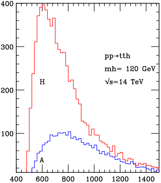
Most of the suggested measurements should be able to verify the CP nature of a Higgs boson when the full luminosity of $300\,$fb^-1 is collected at the LHC or even before, provided the Higgs boson is a CP eigenstate. However, a measurement of the CP mixing is much more difficult, and a combination of several different observables will be essential.

The subject of probing CP mixing reduces more generally to the probing of the anomalous $VVH$ and $t\bar{t}H$ couplings, the only two cases where such study can even be attempted at the LHC. Since CP–even and CP–odd Higgs bosons couple to the $t\bar{t}$ pair democratically where as the coupling to a $VV$ pair is suppressed for the CP–odd case, the most unambiguous in this context will be the $t\bar{t}H$ process [140]. However, as already mentioned a CMS study shows that, at present, it is not clear whether it would be possible to detect the $t\bar{t}H$ signal above the $t\bar{t}b\bar{b}$ background. Hence, $VVH$ is the only relevant case. In principle, the same studies which are used to determine the CP-even or CP-odd character of the Higgs boson mentioned above, can be used.

As an example, we show in Fig. 44 the distribtuion in azimuthal angle $\phi$, for $M_{H}=200$ GeV, where $H$ corresponds to a Higgs which may have indeterminate CP assignments. It should be kept in mind though, that this method cannot be applied for very large Higgs masses where this dependence is washed out. One must also beware of degenerate Higgs bosons of opposite CP; since the decay products are the same, they will both contribute to the rate and must be summed coherently, possibly mimicking the effect seen above. Also, in the context of LHC with the QCD environment and modifications to shapes of distributions, it is useful to construct specific observables which may be directly proportional to the anomalous part of the coupling, as was done in the $e^{+}e^{-}$ case recently [145].

Parameterising the anomalous vertex by

References

- [1] P.W. Higgs, Phys. Lett. 12 (1964) 132; Phys. Rev. Lett. 13 (1964) 506; F. Englert and R. Brout, Phys. Rev. Lett. 13 (1964) 321; G. Guralnik, C. Hagen and T. Kibble, Phys. Rev. Lett. 13 (1964) 585.
- [2] Y. Nambu, Phys. Rev. Lett. 4 (1960) 380; Y. Nambu and G. Jona–Lasinio, Phys. Rev. 122 (1961) 345; ibid Phys. Rev. 124 (1961) 246; J. Goldstone, Nuov. Cim. 19 (1961) 154; J. Goldstone, A. Salam and S. Weinberg, Phys. Rev. 127 (1962) 965.
- [3] For a review on the Higgs sector, see: J. Gunion, H. Haber, G. Kane and S. Dawson, “The Higgs Hunter’s Guide”, Addison–Wesley, Reading 1990.
- [4] A. Djouadi, Phys. Rept. 457 (2008) 1, [arXiv:hep-ph/0503172].
- [5] The LEP collaborations and the LEP electroweak working group, hep-ex/0612034; http://lepewwg.web.cern.ch/LEPEWWG/ .
- [6] LEP working group for Higgs searches, R. Barate et al., Phys. Lett. B565 (2003) 61.
- [7] A. Duperrin, arXiv:0805.3624 [hep-ex].
- [8] C. Amsler et al. (Particle Data Group), Phys. Lett. B667 (2008) 1.
- [9] H. Flaecher et al., arXiv:0811.0009 [hep-ph].
- [10] B.W. Lee, C. Quigg and H.B. Thacker, Phys. Rev. D16 (1977) 1519.
- [11] C.H. Llewellyn Smith, Phys. Lett. B46 (1973) 233; J. S. Bell, Nucl. Phys. B60 (1973) 427 ; J. Cornwall et al, Phys. Rev. Lett. 30 (1973) 1268; Phys. Rev. D10 (1974) 1145.
- [12] N. Cabibbo et al, Nucl. Phys. B158 (1979) 295.
- [13] M. Lüscher and P. Weisz, Phys. Lett. B212 (1988) 472; M. Göckeler et al, Nucl. Phys. B404 (1993) 517; U. Heller et al, Nucl. Phys. B405 (1993) 555.
- [14] T. Hambye and K. Riesselmann, Phys. Rev. D55 (1997) 7255.
- [15] A. Djouadi, M. Spira and P. Zerwas, Z. Phys. C70 (1996) 427; A. Djouadi, J. Kalinowski and P. Zerwas, Z. Phys. C70 (1996) 435.
- [16] A. Djouadi, J. Kalinowski and M. Spira, Comput. Phys. Commun. 108 (1998) 56.
- [17] See e.g. M. Drees, R.M. Godbole and P. Roy, Theory and phenomenology of sparticles, World Scientific, 2005; H. Baer and X. Tata, “Weak scale Supersymmetry: From superfields to scattering events,” Cambridge, UK: Univ. Pr. (2006) .
- [18] A. Djouadi, Phys. Rept. 459 (2008) 1; [arXiv:hep-ph/0503173].
- [19] S. Heinemeyer, W. Hollik and G. Weiglein, Phys. Rept. 425 (2006) 265; B.C. Allanach et al., JHEP 0409 (2004) 044.
- [20] The LEP Collaboration (ALEPH, DELPHI, L3, OPAL), Eur. Phys. J. C47 (2006) 547.
- [21] G. Bélanger et al., Nucl. Phys. B581 (2000) 3, [arXiv:hep-ph/0002039]; G. Belanger et al., Phys. Lett. B 519 (2001) 93; [arXiv:hep-ph/0106275].
- [22] F. Moortgat, hep-ph/0105081; F. Moortgat, S. Abdullin, D. Denegri, hep-ph/0112046.
- [23] See, e.g.: J.I. Illana et al., Eur. Phys. J.C1 (1998) 149; A. Djouadi, Phys. Lett. B435 (1998) 101.
- [24] For a recent status see: S. J. Huber, M. Pospelov and A. Ritz, Phys. Rev. D75 (2007) 036006.
- [25] For a recent review and additional references see: J. M. Cline, arXiv:hep-ph/0609145.
- [26] E. Accomando et al., arXiv:hep-ph/0608079.
- [27] R. M. Godbole, Pramana 67 (2006) 835.
- [28] A. Pilaftsis and C.. Wagner, Nucl. Phys. B553 (1999) 3; M. Carena et al, Nucl. Phys. B586, (2000) 92; S.Y. Choi, M. Drees and J.S. Lee, Phys. Lett. B481 (2000) 57; J. R. Ellis, J. S. Lee and A. Pilaftsis, Mod. Phys. Lett. A21 (2006) 1405.
- [29] M. Carena et al. Nucl. Phys. B659 (2003) 145.
- [30] M. Carena et al, Nucl. Phys. B625 (2002) 345.
- [31] A. Mendez and A. Pomarol, Phys. Lett. B272 (1991) 313, J. Gunion, H. Haber and J. Wudka, Phys. Rev. D43 (1991) 904, B.Grzadkowski, J.Gunion and J. Kalinowski, Phys. Rev. D60 (1999) 075011.
- [32] J.F. Gunion, B. Grzadkowski, H.E. Haber and J. Kalinowski, Phys. Rev. Lett. 79 (1997) 982.
- [33] G. Abbiendi et al. [OPAL Collaboration], Eur. Phys. J. C37 (2004) 49.
- [34] J. R. Ellis, J. S. Lee and A. Pilaftsis, Phys. Rev. D70 (2004) 075010; S.Y. Choi et al, Eur. Phys. J. C40 (2005) 555.
- [35] U. Ellwanger, M. Rausch de Traubenberg and C.A. Savoy, Phys. Lett. B315 (1993) 331, Z. Phys. C67 (1995) 665, Nucl. Phys. B492 (1997) 21; T. Elliott, S.F. King and P. White, Phys. Lett. B351 (1995) 213; S.F. King and P. White, Phys. Rev. D52 (1995) 4183.
- [36] J. Kim and H. Nilles, Phys. Lett. B138 (1984) 150.
- [37] A. Djouadi, U. Ellwanger and A. Teixeira, Phys. Rev. Lett. 101 (2008) 101802.
- [38] For recent analyses, see: U. Ellwanger and C. Hugonie, Eur. Phys. J. C25 (2002) 297; U. Ellwanger et al., hep-ph/0111179 and hep-ph/0305109; U. Ellwanger, C. Hugonie and J. Gunion, JHEP 0502 (2005) 066; J. Gunion and R. Dermisek, Phys. Rev. Lett. 95 (2005) 041801 ; D.J. Miller, R. Nevzorov and P.M. Zerwas, Nucl. Phys. B681 (2004) 3; V. Barger et al., Phys. Rev. D73 (2006) 115010; C. Balazs and D. Carter, arXiv:0808.0770 [hep-ph].
- [39] For a recent discussion and more references, see A. Djouadi et al., JHEP 0807 (2008) 002 [arXiv:0801.4321 [hep-ph]].
- [40] See e.g., P.N. Pandita, Pramana 51 (1998) 169 and references therein.
- [41] M. Drees et al., Phys. Lett. B433 (1998) 346.
- [42] See e.g. S. King, S. Moretti and R. Nevzorov, Phys. Rev. D73 (2006) 035009.
- [43] See e.g. T. Han, P. Langacker and B. McElrath, Phys. Rev. D70 (2004) 115006.
- [44] See, for example, R. Godbole et al, Phys. Lett. B 352 (1995) 388; J. Gunion hep-ph/0212150; T. Han et al, Phys. Rev. D 76 (2007) 075013.
- [45] See e.g., J. Espinosa and M. Quiros, Phys. Rev. Lett. 81 (1998) 516.
- [46] M. Hirsch, et al, Phys. Rev. D73 (2006) 055007; A. Villanova del Moral in Ref. [26].
- [47] L. Randall and R. Sundrum, Phys. Rev. Lett. 83 (1999) 3370.
- [48] J. L. Hewett and T. G. Rizzo, JHEP 0308 (2003) 028.
- [49] M. Chaichian et al, Phys. Lett. B524 (2002) 161.
- [50] D. Dominici et al, Nucl. Phys. B671 (2003) 243.
- [51] N. Arkani-Hamed, S. Dimopoulos and G. Dvali, Phys. Lett. B429, (1998) 263 and Phys. Rev. D59 (1999) 086004; A. Antoniadis et al, Phys. Lett. B436 (1998) 257.
- [52] G. Giudice, R. Rattazi and J. Wells, Nucl. Phys. 595 (2001) 250; M. Battaglia et al, hep-ph/0402062.
- [53] J. van der Bij, Phys. Lett. B636 (2006) 56; S. Dilcher and J. van der Bij, Phys. Lett. B638 (2006) 234; see also, J. Kumar and J.D. Wells, Phys. Rev. D74 (2006) 115017.
- [54] See, e.g. D. Choudhury, A. Datta and K. Huitu, Nucl. Phys. B673 (2003) 385.
- [55] N. Arkani-Hamed et al., JHEP 0208 (2002) 021; N. Arkani-Hamed et al, JHEP 0207 (2002) 034.
- [56] S. Weinberg, Phys. Rev. D13 (1979) 974 and Phys. Rev. D19 (1979) 1277; L. Susskind, Phys. Rev. D20 (1979) 2619; For a review: C. Hill and E. Simmons, Phys. Rept. 381 (2003) 235.
- [57] W. Kilian, D. Rainwater and J. Reuter, Phys. Rev. D74, (2006) 095003, [Erratum-ibid. D74 (2006) 099905]; ibid. D71 (2005) 015008.
- [58] G. Giudice et al, JHEP 0706 (2007) 045.
- [59] C. Csaki et al., Phys. Rev. D69 (2004) 055006; C. Csaki et al, Phys. Rev. Lett. 92 (2004) 101802.
- [60] See e.g., A. Birkedal, K. Matchev and M. Perelstein, Phys. Rev. Lett. 94 (2005) 191803.
- [61] H. Georgi et al., Phys. Rev. Lett. 40 (1978) 692; S.L. Glashow, D.V. Nanopoulos and A. Yildiz, Phys. Rev. D18 (1978) 1724; R.N. Cahn and S. Dawson, Phys. Lett. B136 (1984) 196; K. Hikasa, Phys. Lett. B164 (1985) 385; G. Altarelli, B. Mele and F. Pitolli, Nucl. Phys. B287 (1987) 205; Z. Kunszt, Nucl. Phys. B247 (1984) 339; J. Gunion, Phys. Lett. B261 (1991) 510.
- [62] M. Spira, http://mspira.home.cern.ch/ mspira/proglist.html.
- [63] A.D. Martin et al. [MRST Collaboration], Eur. Phys. J. C28 (2003) 455.
- [64] See e.g., J.F. Gunion et al., Phys. Rev. D34 (1986) 101; J. Gunion, G. Kane and J. Wudka, Nucl. Phys. B299 (1988) 231; M. Dittmar and H. Dreiner, Phys. Rev. D55 (1997) 167.
- [65] ATLAS Collaboration, Technical Design Report, CERN/LHCC/99-15 (1999).
- [66] CMS Collaboration, Physics TDR, CERN/LHCC/2006-021, June 2006.
- [67] E. Richter–Was et al., Int. J. Mod. Phys. A13 (1998) 1371, ATLAS Note PHYS–No–074. D. Denegri et al. hep-ph/0112045 and CMS–Note 2003/033; G. Branson et al. (CMS and ATLAS Collaborations), Eur. Phys. J. direct C4 (2002) N1; S. Asai et al., Eur. Phys. J. C32S2 (2004) 19; V. Büscher and K. Jakobs, Int. J. Mod. Phys. A20 (2005) 2523.
- [68] Proceedings of the Les Houches Workshops on “Physics at TeV Colliders”: A. Djouadi et al. (1999), hep-ph/0002258 ; D. Cavalli et al. (2001), hep-ph/0203056; K.A. Assamagan et al. (2003), hep-ph/0406152; C. Buttar et al., hep-ph/0604120 (2005).
- [69] Proceedings of the Les Houches Workshop 2007,N.E. Adam et al., arXiv:0803.1154 [hep-ph].
- [70] G. Weiglein et al., “LHC/LC Study Group”, Phys. Rept. 426 (2006) 47.
- [71] A. Djouadi, M. Spira and P. Zerwas, Phys. Lett. B264 (1991) 440; S. Dawson, Nucl. Phys. B359 (1991) 283.
- [72] M. Spira et al., Nucl. Phys. B453 (1995) 17; Phys. Lett. B318 (1993) 347.
- [73] R.V. Harlander and W. Kilgore, Phys. Rev. Lett. 88 (2002) 201801; C. Anastasiou and K. Melnikov, Nucl. Phys. B646 (2002) 220. V. Ravindran, J. Smith and W.L. Van Neerven, Nucl. Phys. B665 (2003) 325.
- [74] S. Moch and A. Vogt, Phys. Lett. B631 (2005) 48; S. Marzani et al., Nucl. Phys. B800 (2008) 127 and arXiv:0809.4934 [hep-ph]; V. Ahrens et al., arXiv:0808.3008 [hep-ph] and arXiv:0809.4283 [hep-ph].
- [75] C. Anastasiou, K. Melnikov and F. Petriello, Nucl. Phys. B724 (2005) 197; C. Anastasiou, G. Dissertori and F. Stockli, JHEP 0709 (2007) 018; S. Catani and M. Grazzini, Phys. Rev. Lett. 98 (2007) 222002; M. Grazzini, JHEP 0802 (2008) 043.
- [76] S. Catani et al, JHEP 0307 (2003) 028.
- [77] C.R. Schmidt, Phys. Lett. B413 (1997) 391; D. de Florian, M. Grazzini and Z. Kunszt, Phys. Rev. Lett. 82 (1999) 5209. C. Balazs and C. P. Yuan, Phys. Lett. B478 (2000) 192; C. J. Glosser and C. R. Schmidt, JHEP 0212 (2002) 016; E. L. Berger and J. W. Qiu, Phys. Rev. D67 (2003) 034026; A. Kulesza, G. Sterman, W. Vogelsang, Phys. Rev. D69 (2004) 014012; G. Bozzi et al, Phys. Lett. B564 (2003) 65; V. Ravindran, J. Smith and W.L. Van Neerven, Mod. Phys. Lett. A18 (2003) 1721; C. Anastasiou, L. Dixon and K. Melnikov, Nucl. Phys. Proc. Suppl. 116 (2003) 193; C.Anastasiou K. Melnikov and F. Petriello, Phys. Rev. Lett. 93 (2004) 262002; J. Campbell, R. Ellis and G. Zanderighi, JHEP 0610 (2006) 028; J. Butterworth et al., Phys. Rev. Lett. 100 (2008) 242001.
- [78] A. Djouadi and P. Gambino, Phys. Rev. Lett. 73 (1994) 2528; U. Aglietti et al. Phys. Lett. B595 (2004) 432; G. Degrassi and F. Maltoni, Phys. Lett. B600 (2004) 255; S. Actis et al., arXiv:0809.3667 [hep-ph].
- [79] G. Altarelli, R.K. Ellis and G. Martinelli, Nuc. Phys. B157 (1979) 461; J. Kubar–André and F. Paige, Phys. Rev. D19 (1979) 221; T. Han and S. Willenbrock, Phys. Lett. B273 (1991) 167; J. Ohnemus and W. J. Stirling, Phys. Rev. D47 (1993) 2722;
- [80] For a review of NLO QCD corrections, see: M. Spira, Fortschr. Phys. 46 (1998) 203; see also: hep-ph/9711394 and hep-ph/9810289; A. Djouadi and M. Spira, Phys. Rev. D62 (2000) 014004.
- [81] O. Brein, A. Djouadi and R. Harlander, Phys. Lett. B579 (2004) 149.
- [82] M. L. Ciccolini, S. Dittmaier and M. Krämer, Phys. Rev. D68 (2003) 073003.
- [83] T. Han, G. Valencia and S. Willenbrock, Phys. Rev. Lett. 69 (1992) 3274.
- [84] M. Ciccolini, A. Denner and S. Dittmaier, Phys. Rev. Lett. 99 (2007) 161803 and Phys. Rev. D77 (2008) 013002.
- [85] T. Figy, C. Oleari and D. Zeppenfeld. Phys. Rev. D68 (2003) 073005.
- [86] V. Barger et al., Phys. Rev. D44 (1991) 1426; V. Barger, R. Phillips, D. Zeppenfeld, Phys. Lett. B346 (1995) 106; D. Rainwater and D. Zeppenfeld JHEP 9712 (1997)005.
- [87] D. Zeppenfeld et al, Phys. Rev. D62 (2000) 013009 and in the first report of Ref. [68].
- [88] M. Dührssen et al., Phys. Rev. D70 (2004) 113009.
- [89] T. Plehn, D. Rainwater and D. Zeppenfeld, Phys. Rev. D61 (2000) 093005; N. Kauer et al, Phys. Lett. B503 (2001) 113; T. Plehn and D. Rainwater, Phys. Lett. B520 (2001) 108; M.L. Mangano et al., Phys. Lett. B556 (2003) 50.
- [90] O. Eboli and D. Zeppenfeld, Phys. Lett. B495 (2000) 147.
- [91] W. Beenakker et al., Phys. Rev. Lett. 87 (2001) 201805; Nucl. Phys. B653 (2003) 151; S. Dawson et al., Phys. Rev. Lett. 87 (2001) 201804 and Phys. Rev. D67 (2003) 071503.
- [92] S. Dittmaier, M. Krämer and M. Spira, Phys. Rev. D70 (2004) 074010; S. Dawson et al, Phys. Rev. D69 (2004) 074027.
- [93] J. Campbell et al, Phys. Rev. D67 (2003) 095002; R. Harlander and W. Kilgore, Phys. Rev. D68 (2003) 013001; F. Maltoni, Z. Sullivan and S. Willenbrock Phys. Rev. D67 (2003) 093005; E. Boos and T. Plehn, Phys. Rev. D69 (2004) 094005.
- [94] T. Plehn, Phys. Rev. D67 (2003) 014018.
- [95] J. Campbell et al. in Ref. [68] 2001.
- [96] A. Djouadi and S. Ferrag, Phys. Lett. B586 (2004) 345.
- [97] A. Djouadi, arXiv:0810.2439 [hep-ph].
- [98] For recent reviews and a summary of recent developments, see: R. Harlander, J.Phys.G35 (2008) 033001; M. Mühlleitner, arXiv:0810.1158.
- [99] C. Kao, Phys. Rev. D46 (1992) 4907 and Phys. Lett. B328 (1994) 420; Y. Jun et al., hep-ph/0209279; C. Kao, G. Lovelace and L.H. Orr, Phys. Lett. B567 (2003) 259; O. Brein and W. Hollik, Phys. Rev. D68 (2003) 095006 (2003); B. Field et al., Phys. Lett. B551 (2003) 137; B. Field, S. Dawson and J. Smith, Phys. Rev. D69 (2004) 074013; Q.H. Cao, S. Kanemura and C.P. Yuan, Phys. Rev. D69 (2004) 075008; U. Langenegger et al, JHEP 0606 (2006) 035.
- [100] A. Bawa, C. Kim and A. Martin, Z. Phys. C47 (1990) 75; V. Barger, R. Phillips and D.P. Roy, Phys. Lett. B324 (1994) 236; S. Moretti and K. Odagiri, Phys. Rev. D55 (1997) 5627; J. Gunion, Phys. Lett. B322 (1994) 125; F. Borzumati, J.L. Kneur and N. Polonsky, Phys. Rev. D60 (1999) 115011; D. Miller et al, Phys. Rev. D61 (2000) 055011; D.P. Roy, Phys. Lett. B459 (1999) 607.
- [101] For a review, see S. Moretti, Pramana 60 (2003) 369
- [102] E. Boos, A. Djouadi and A. Nikitenko, Phys. Lett. B578 (2004) 384.
- [103] E. Boos et al., Phys. Rev. D66 (2002) 055004; E. Boos et al., Phys. Lett. B622 (2005) 311; A. Djouadi and Y. Mambrini, JHEP 0612 (2006) 001.
- [104] V. Barger and C. Kao, Phys. Lett. B424 (1998) 69; Tao Han and B. McElrath, Phys. Lett. B528 (2002) 81; S. Dawson, D. Dicus and C. Kao, Phys. Lett. B545 (2002) 132.
- [105] D.P. Roy, Mod. Phys. Lett. A19 (2004) 1813.
- [106] A. Djouadi, J.L. Kneur, G. Moultaka, Phys. Rev. Lett. 80 (1998) 1830 and Nucl. Phys. B569 (2000) 53; G. Belanger, F. Boudjema and K. Sridhar, Nucl. Phys. B568 (2000) 3; A. Dedes and S. Moretti, Eur. Phys. J. C10 (1999) 515 and Phys. Rev. D60 (1999) 015007.
- [107] Asesh Datta et al., Phys. Rev. D65 (2002) 015007; Asesh Datta et al., Nucl. Phys. B681 (2004) 31.
- [108] A. Dedes and S. Moretti, Phys. Rev. Lett. 84 (2000) 22; Nucl. Phys. B576 (2000) 29.
- [109] S. Moretti, S. Munir and P. Poulose, Phys. Lett. B649 (2007) 206; S. Hesselbach et al, Eur. Phys. J. C54 (2008) 129.
- [110] S.Y. Choi, K. Hagiwara and J.S. Lee, Phys. Rev. D64 (2001) 032004; Phys. Lett. B529 (2002) 212; A. G. Akeroyd and A. Arhrib, Phys. Rev. D64 (2001) 095018; A. Arhrib, D. K. Ghosh and O. C. W. Kong, Phys. Lett. B537 (2002) 217; S. Y. Choi et al, Eur. Phys. J. C25 (2002) 307.
- [111] D. K. Ghosh, R. M. Godbole and D. P. Roy, Phys. Lett. B628 (2005) 131, [arXiv:hep-ph/0412193].
- [112] J. S. Lee et al. Comput. Phys. Commun. 156 (2004) 283; S. Heinemeyer, W. Hollik and G. Weiglein, Comp. Phys. Commun. 124 (2000) 76.
- [113] M. Schumacher, hep-ph/0410112.
- [114] R. M. Godbole and D. P. Roy, in Ref. [26].
- [115] P. Bandyopadhyay et al., Phys. Rev. D78 (2008) 015017.
- [116] J. Gunion, Phys. Rev. Lett. 72 (1994) 199.
- [117] D. Choudhury and D.P. Roy, Phys. Lett. B322 (1994) 368.
- [118] R. M. Godbole et al., Phys. Lett. B571 (2003) 184.
- [119] H. Davoudiasl, T. Han and H. Logan, Phys. Rev. D71 (2005) 115007.
- [120] B. Di Girolamo et al., in Ref. [68] (2001), G. Bélanger et al. in [68] (2001), S. Balatenychev et al., in [68] (2001).
- [121] A. Djouadi and G. Moreau, Phys. Lett. B660 (2008) 67 [arXiv:0707.3800 [hep-ph]].
- [122] A. Djouadi et al. [ILC Collaboration], arXiv:0709.1893 [hep-ph].
- [123] E. Glover and J. van der Bij, Nucl. Phys. B309 (1988) 282; T. Plehn, M. Spira and P. Zerwas, Nucl. Phys. B479 (1996) 46; M. Muhlleitner et al., Eur. Phys. J. C10 (1999) 45.
- [124] U. Baur, T. Plehn and D. L. Rainwater, Phys. Rev. Lett. 89 (2002) 151801; Phys. Rev. D67 (2003) 033003; Phys. Rev. D69 (2004) 053004.
- [125] R. Kinnunen, S. Lehti, F. Moortgat, A. Nikitenko and M. Spira in Ref. [68] (2003).
- [126] R. M. Godbole et al., arXiv:hep-ph/0404024.
- [127] V. Barger et al., Phys. Rev. D49 (1994) 79.
- [128] S. Y. Choi et al, Phys. Lett. B553 (2003) 61.
- [129] C. P. Buszello et al., Eur. Phys. J. C32 (2004) 209; C. P. Buszello and P. Marquard, in Ref. [26]; C. P. Buszello, P. Marquard and J. J. van der Bij, arXiv:hep-ph/0406181.
- [130] R. M. Godbole et al, Pramana 67 (2006) 617; ibid. in Ref. [26].
- [131] R. M. Godbole, D. J. Miller and M. M. Muhlleitner, JHEP 0712 (2007) 031; [arXiv:0708.0458 [hep-ph]].
- [132] T. Plehn, D. Rainwater and D. Zeppenfeld, Phys. Rev. Lett. 88 (2002) 051801.
- [133] B. Zhang et al, Phys. Rev. D67 (2003) 114024.
- [134] C. P. Buszello and P. Marquard, arXiv:hep-ph/0603209.
- [135] V. Del Duca et al., arXiv:hep-ph/0109147.
- [136] V. Hankele, G. Klamke and D. Zeppenfeld, arXiv:hep-ph/0605117; V. Hankele et al, Phys. Rev. D74 (2006) 095001.
- [137] K. Odagiri, JHEP 0303 (2003) 009.
- [138] W. Bernreuther, M. Flesch and P. Haberl, Phys. Rev. D58 (1998) 114031. W. Bernreuther, A. Brandenburg and M. Flesch, arXiv:hep-ph/9812387.
- [139] W. Khater and P. Osland, Nucl. Phys. B661 (2003) 209.
- [140] J. F. Gunion and X. G. He, Phys. Rev. Lett. 76 (1996) 4468; J. Albert et al., in Ref. [26]; B. Field, Phys. Rev. D 66 (2002) 114007.
- [141] V. A. Khoze et al, Eur. Phys. J. C 23 (2002) 311; A. De Roeck et al, Eur. Phys. J. C 25 (2002) 391.
- [142] J. R. Ellis et al, Phys. Rev. D 71 (2005) 075007.
- [143] P. S. Bhupal Dev et al., Phys. Rev. Lett. 100 (2008) 051801 [arXiv:0707.2878 [hep-ph]].
- [144] A. Djouadi et al., in preparation.
- [145] S. S. Biswal et al, Phys. Rev. D73 (2006) 035001, [Erratum-ibid. D74 (2006) 039904] [arXiv:hep-ph/0509070]; S. S. Biswal et al, arXiv:0809.0202 [hep-ph].
- [146] S. Dutta et al, Phys. Rev. D 78 (2008) 115016.