ASKI: full-sky lensing map making algorithms
Abstract
Within the context of upcoming full-sky lensing surveys, the edge-preserving non-linear algorithm Aski (All Sky Inversion) is presented. Using the framework of Maximum A Posteriori inversion, it aims at recovering the optimal full-sky convergence map from noisy surveys with masks. Aski contributes two steps: (i) CCD images of possibly crowded galactic fields are deblurred using automated edge-preserving deconvolution; (ii) once the reduced shear is estimated using standard techniques, the partially masked convergence map is also inverted via an edge-preserving method.
The efficiency of the deblurring of the image is quantified by the relative gain in the quality factor of the reduced shear, as estimated by Sextractor. Cross validation as a function of the number of stars removed yields an automatic estimate of the optimal level of regularization for the deconvolution of the galaxies. It is found that when the observed field is crowded, this gain can be quite significant for realistic ground-based eight-metre class surveys. The most significant improvement occurs when both positivity and edge-preserving penalties are imposed during the iterative deconvolution.
The quality of the convergence inversion is investigated on noisy maps derived from the horizon-4 N-body simulation with SNR within the range , with and without Galactic cuts, and quantified using one-point statistics ( and ), power spectra, cluster counts, peak patches and the skeleton. It is found that (i) the reconstruction is able to interpolate and extrapolate within the Galactic cuts/non-uniform noise; (ii) its sharpness-preserving penalization avoids strong biasing near the clusters of the map (iii) it reconstructs well the shape of the PDF as traced by its skewness and kurtosis (iv) the geometry and topology of the reconstructed map is close to the initial map as traced by the peak patch distribution and the skeleton’s differential length (v) the two-points statistics of the recovered map is consistent with the corresponding smoothed version of the initial map (vi) the distribution of point sources is also consistent with the corresponding smoothing, with a significant improvement when prior is applied. The contamination of B-modes when realistic Galactic cuts are present is also investigated. Leakage mainly occurs on large scales. The non-linearities implemented in the model are significant on small scales near the peaks in the field.
Keywords:
Cosmology, Inverse methods, Lensing. Dark energy. 10/10/081 Introduction
In recent years, weak shear measurements have become a major source of cosmological information. By measuring the bending of the rays of light emerging from distant galaxies, one can gain some knowledge of the distribution of matter between the emitter and ourselves, and thus probe the properties and evolution history of dark matter (Bartelmann & Schneider, 2001). This technique has led to significant results in a broad spectrum of topics, from measurements of the projected dark matter power spectrum (for the latest results see Fu & et al. (2008)), 3D estimation of the dark matter spectrum (Kitching et al., 2006), studies of the higher order moments of the dark matter distribution, selection of source candidates for subsequent follow-ups (Schirmer et al., 2007), and reconstruction of the mass distribution from small (Jee et al., 2007) to large scales (Massey et al., 2007). In view of these successes, numerous surveys have been planned specifically to use this probe either from ground-based facilities (eg VST-KIDS11 1 http://www.astro-wise.org/projects/KIDS/, DES22 2 https://www.darkenergysurvey.org/ Pan-STARRS33 3 http://pan-starrs.ifa.hawaii.edu/, LSST44 4 http://www.lsst.org/) or space-based observatories (EUCLID55 5 http://www.dune-mission.net/, SNAP66 6 http://snap.lbl.gov/ and JDEM77 7 http://universe.nasa.gov/program/probes/jdem.html). More generally, it is clear that weak lensing will be a major player in the future, as it has been identified by different European and US working groups as one of the most efficient way of studying the properties of dark energy88 8 see, on the European side http://www.stecf.org/coordination/ and on the US side, http://www.nsf.gov/mps/ast/aaac.jsp and http://www.nsf.gov/mps/ast/detf.asp. Data processing is an important issue in the exploitation of weak lensing of distant galaxies. The signal comes from the excess alignment of the ellipticities of the observed galaxies. Assuming one can ignore or deal with spurious alignments due to intrinsic effects (Hirata & Seljak, 2004; Aubert et al., 2004; Pichon & Bernardeau, 1999), or due to spurious lensing effects (Bridle & Abdalla, 2007), the weak lensing signal will thus come from a small statistically coherent ellipticity on top of the random one of each object. Any result obtained with weak lensing on distant galaxies is thus conditioned by the quality with which shape parameters of the galaxies are recovered. This issue has of course been raised by the weak lensing community and tackled by the SHear Testing Program working group (Massey, 2007; Heymans, 2006) whose effort have allowed for a fair comparison of the existing techniques. Schematically, the measurement of the shape parameters of the galaxies can be seen as a two-step process. First, one must correct for the non-idealities of the images due to atmospherical seeing (for ground-based telescopes), and telescope and camera aberrations. Indeed, these effects translate into an asymmetrical beam, which is varying between two images, and even possibly in the field of one image. Typically, the asymmetry induced by the instrumental response is much larger than the ellipticity to be measured. After this preprocessing step, a shape determination algorithm can be applied, and some estimation of the ellipticity of the object recovered. Stars, defects in the images, and objects too close to each other after deconvolution have to be removed from the final catalogue so as to avoid contamination from erroneous shape measurements.
After these operations, one obtains a catalogue of position and shape parameters. Many techniques exist for recovering the weak shear signal from this catalogue. For example, a lot of efforts have been devoted to the measurement of the shear two-point functions. The most used method is the two-point functions; however measurement of the so called Mass Aperture averaged two-point function, which is the result of the convolution of the shear two-point functions by a compensated filter (Schneider et al., 2002) is becoming the preferred method (Fu & et al., 2008). This scheme includes the separation between the curl-free convergence-field two-point function, and the residual curl mode that can arise from incomplete PSF correction or intrinsic galaxy alignment (Crittenden et al., 2002). For three-point functions, different resummation schemes have been proposed, either using direct measurement of the shear (Bernardeau et al., 2002; Benabed & Scoccimarro, 2005) or using the Mass Aperture filter (Takada & Jain, 2003; Kilbinger & Schneider, 2005).
Other applications (source detection and fit, some tomography algorithms) call for an estimation of the map of the convergence field. A convergence map can also be used to measure the two- and three-point functions as well, even if, as we will see later this is not optimal. For these reasons an important amount of work has already been devoted to the reconstruction of the convergence map (van Waerbeke et al., 1999; Seitz et al., 1998; Bartelmann et al., 1996). The problem in this reconstruction lies in the inversion of the non-local equations linking the convergence field , and the ellipticities of the galaxies, while controlling the noise and avoiding pollution from the spurious curl modes. Moreover, even assuming that the ellipticity catalogue was a noise free estimation of a curl-free underlying shear, the inversion could only be exact up to a global translation given the functional form of the equation. Thus Bayesian techniques that use a priori properties on the solution to regularize the inversion problem are well suited to the reconstruction of . Previous works on the topic have explored different sets of a priori and regularization techniques (Marshall et al., 2002; Starck et al., 2005; Seitz et al., 1998; Bridle et al., 1998). The primary goal of those investigations being the measurement of the mass distribution in clusters, most of them are dealing only with finite regions of the sky. For the same reason those papers have been extended to include strong-lensing effects that can be observed around the cluster whose mass is being reconstructed using their lensing effect (Cacciato et al., 2006; Bradac et al., 2005; Halkola et al., 2006; Jee et al., 2007).
In this paper, we will focus on the optimal reconstruction of the field from very large, and possibly full-sky maps, of the sky. We will thus only be interested in the weak lensing regime including the onset of the quasi-linear regime, where the non-linearities of the relation linking the ellipticities of the galaxies to the shear cannot be safely neglected. We will propose a self calibrated regularization technique, that can be compared to multi resolution methods or wavelet approach (Starck et al., 2005; Abrial et al., 2008), and use a regularization scheme to perform a sharp feature preserving inversion. One of the biggest issues we will have to cope with is the incomplete coverage of the sky. We will show how our technique can deal with irregular coverage and masked portions of the sky.
Specifically, Section 2
shows how self calibrated non-parametric deblurring can improve
the construction of reduced shear, hence convergence maps. Section
3 describes the model for the reduced shear,
the corresponding inverse problem, and the optimization procedure. Section
4 investigates the quality of the global reconstruction;
in particular, it probes the asymmetry/kurtosis of the recovered maps,
its topology (total length and differential length of the skeleton), the
recovered power spectra, the point source catalogue with and without
galactic star cut. The leaking of B-modes induced by the Galactic
cut is also investigated. Finally, Section 5 discusses
implications for upcoming full-sky surveys and wraps up.
Appendix A describes the
star removal algorithm (implemented for the cross validation estimation of the optimal level of smoothing
required to deconvolve the crowded images), Appendix B details the inverse problem on the sphere
while Appendix C derives the local plane corresponding approximation. Appendix D
describes the construction of realistic maps from large N-body simulations.
2 Deblurring of crowded fields
The first step involved in reconstructing a full-sky map of the convergence on the sky requires estimating ellipticity and orientation maps from wide angle CCD images of large patches of the sky. Whether the experiment is ground-based, or space-born, it is advisable to correct for the effect of the instrumental response, in particular when mapping more crowded regions closer to the galactic plane. Indeed, the PSF-induced partial overlapping of galaxies within the field of view will bias the estimation of the reduced shear. What we will describe here would correspond to a method belonging to the “orange” quadrant of the classification proposed in table 3 of Massey (2007). Current methods have been designed for deblurring of isolated objects and are consequently less efficient in deblurrinng blended objects. As a first step towards building a full-sky map maker, let us therefore address the issue of deblurring crowded fields via regularized non parametric model fitting, and assess its efficiency in the weak lensing context.
In particular we will show that cross validation as a function of the number of stars removed yields an automatic estimate of the optimal level of regularization for the deconvolution of the galaxies. When the observed field is crowded, this gain can be quite significant for realistic ground-based eight-metre class surveys. The most significant improvement occurs when both positivity and edge-preserving penalties are imposed during th e iterative deconvolution.
2.1 Deblurring as an inverse problem
2.1.1 Regularized solution
Since observed objects are incoherent sources, the observed image depends linearly on the sky brightness distribution:
where is the observed distribution in the direction , is the atmospheric and instrumental point spread function (PSF) which is the distribution of observed light in the direction due to light coming from direction , is the true sky brightness distribution and is the noise. After discretization:
| (1) |
where is the vector of pixel intensities in the observed image (the data), is the matrix which accounts for the atmospheric and instrumental blurring, is the (discretized or projected onto a basis of functions) object brightness distribution and accounts for the errors (pixel-wise noise and modelisation approximations). Deblurring requires estimating the best sky brightness distribution given the data. Since the atmospheric and instrumental PSF results in a smoother distribution than the true one, it is well known that de-blurring is an ill-conditioned problem ((Richardson, 1972; Skilling et al., 1979; Tarantola & Valette, 1982; Pichon & Thiébaut, 1998; Pichon et al., 2001)). In other words, straightforward deblurring by applying to the data would result in uncontrolled amplification of noise: a small change in the input data would yield unacceptably large artifacts in the solution. Regularization must be used to overcome ill-conditioning of this inverse problem. This is achieved by using additional prior constraints such as requiring that the solution be as smooth as possible, while being still in statistical agreement with the data and while imposing that the brightness distribution is positive. Following this prescription, the Maximum A Posteriori (MAP) solution is the one which minimizes an objective function :
| (2) |
where is a likelihood penalty which enforces agreement of the model with the data, is a regularization penalty which enforces prior constraints set on the model, and is a so-called hyper-parameter which allow the tuning of the relative weight of the prior with respect to the data. Hence the MAP solution is a compromise between what can be inferred from the data alone and prior knowledge about the parameters of interest. Assuming Gaussian statistics for the errors in equation (1), the likelihood penalty writes:
| (3) |
where the weighting matrix is equal to the inverse of the covariance matrix of the errors: .
The most effective regularization for ill-conditioned problems such as deconvolution of blurred images consists in imposing a smoothness constraint (Thiébaut, 2005). Then the regularization penalty writes:
| (4) |
where is the local gradient of and is some cost function. The local gradient of can be approximated by finite differences: where is a linear finite difference operator. For instance, in 1-D: . To enforce smoothness, the cost function must be an increasing function of the magnitude of its argument. Very common choices for are: the norm, the norm, or an norm. For our deblurring problem, we have considered different priors (quadratic or smoothness) possibly with an additional positivity constraint. We have used generalized cross validation (GCV,(Wahba, 1990)) applied to the circulant approximation of the quadratic problem to estimate the optimal regularization level . These different possibilities and their effects on the recovered images are discussed in details in what follows.
Finally, to solve for the constrained optimization problem (2), we used the vmlmb algorithm from OptimPack (Thiébaut, 2002). Vmlmb (for Variable Metric, Limited Memory, Bounded) makes use of a BFGS (Nocedal & Wright, 2006) update of the approximation of the Hessian (matrix of second partial derivatives) of to derive a step to improve the parameters at every iteration. This strategy only requires computing the objective function, , and its gradient (partial derivatives) with respect to the parameters . The BFGS update is limited to a few last steps so that the memory requirements remains modest, that is a few times the number of sought parameters, and the algorithm can be applied to solve very large problems (in our case, there are as many parameters as the number of pixels in the sought image). Finally, Vmlmb accounts for bound constraints by means of gradient projections (Nocedal & Wright, 2006). For a convex penalty , Vmlmb is guaranteed to converge to the unique feasible minimum of which satisfies the bound constraints; for a non-convex penalty, Vmlmb being based on a descent strategy, it will find a local minimum depending on the initial set of parameters.

2.1.2 Quadratic regularization and Wiener proxy
| 128 | 256 | 512 | 1024 | 2048 | |
| time for one step (s) | 0.13 | 0.59 | 2.13 | 8.48 | 34.3 |
| number of steps (s) | 13 | 12 | 9 | 13 | 24 |
| total time (s) | 2.6 | 10.4 | 33.4 | 171.1 | 1129.3 |
Using the finite difference operator and an norm for the regularization and ignoring for the moment the positivity constraint, the MAP solution is the minimum of a quadratic penalty which simply involves solving a (huge) linear problem:
| (5) | |||||
providing the Hessian matrix is non-singular, which is generally the case for Owing to the large size of the matrices involved in this equation (there are as many unknown as the number of pixels), the linear problem has to be iteratively solved (by a limited memory algorithm such as vmlm) unless it can be diagonalized as explained below. The solution, equation (5), involves at least one parameter, , which needs to be set to the correct level of regularization: too low would give a solution plagued by lots of artifacts due to noise amplification, too high would result in an oversmoothed solution with small details blurred. The optimal level of smoothing can be computed by generalized cross validation (GCV) by minimizing with respect to the function (Golub et al., 1979; Wahba, 1990):
| (6) |
where is the number of data (size of ) and is the so-called influence matrix, in our case:
| (7) |
Computing the value of involves: (i) solving the problem to find the regularized solution and compute ; (ii) estimate the trace of perhaps by using Monte Carlo methods (Girard, 1989) since the influence matrix is very large. The computational cost of stages (i) and (ii) is similar to that of a few solvings of the quadratic problem. Since this has to be repeated for every different value of the regularization level, finding the optimal value of by means of GCV can be very time consuming unless the problem can be approximated by a diagonal quadratic problem (for which matrix inversions are both fast and trivial).
For this purpose, we introduce the proxy problem corresponding to white noise and circulant approximations of the operators (convolution by the PSF) and (finite differences). Then the weighting matrix becomes:
where is the variance of the noise. In the special case where the PSF is shift-invariant, is a convolution operator which can be approximated by a block Toeplitz with Toeplitz block matrix that can be coputed very quickly by means of FFT’s:
| (8) |
where is the PSF (the first row of ), is the forward DFT operator, and is the diagonal matrix with its diagonal given by the vector . This discrete convolution equation assumes that where is the length of the dimension, and are the indices of the position and discrete Fourier frequency along this dimension. In this case, the inverse DFT is simply with the total number of elements in and the exponent standing for the conjugate transpose. With these approximations and definitions of the DFT, the likelihood term writes:
| (9) |
where is the transfer function (the DFT of the point spread function) and and respectively the DFT of the data and of the sought image. Note that the exact normalization factor, here , depends on the particular definition of the DFT.
Similarily, ignoring edges effects, the finite difference operator along direction can be approximated by:
| (10) |
where is the DFT of the first row of ; then the quadratic regularization writes:
| (11) |
with:
| (12) |
for first order finite differences and our choice for the DFT. Note that any being an increasing function of the length of the spatial frequency could be used instead and would result in imposing a smoothness constraint although with a different behaviour. Finally putting all these circulant approximations together, the quadratic problem to solve is diagonalized in the DFT space and trivially solved to gives the DFT of the MAP solution:
| (13) |
the asterisk exponent denoting the complex conjugate. Note that this circulant approximation of the solution is very fast to compute as it involves just a few FFT’s. This expression of the MAP solution is very similar to what would give Wiener filter which would be exactly achieved by setting the term equals to the reciprocal of the expected image powerspectrum in equation (13). Since, in our case, the image powerspectrum is unknown a priori, we have to choose the regularization shape and derive the optimal level of smoothing, for instance, by means of GCV. Thanks to the circulant approximation made here, GCV criterion is now very easy to compute as:
and , hence:
| (14) |
with
| (15) |
In practice, for the optimization of equation (2), equation (13) is taken as a starting point together with the choice of given by the minimum of equation (14). Then the optimization of equation (2) is carried with possibly non stationary weights, while iterating back and forth between model and data space.

2.1.3 Crowded fields and star removal
Even though the estimation of the ellipticities does not require per se the deconvolution of the galaxies, it is shown below that this estimation is significantly improved by deconvolution when the fields of view are crowded and polluted by foreground stars: indeed galaxies and stars overlap less when deconvolved, which reduces the fraction of erroneous measurements. Unfortunately, when these stars are present, they significantly bias the estimation of the hyper parameter, , since stars correspond to high frequency correlated signal which leads to an underestimation of the optimal level of smoothing (for the galaxies) by cross validation. This is best seen in Figure 1 which displays the evolution of the hyper-parameter which minimizes GCV as a function of the number of stars removed by our star removal algorithm, see Appendix A. Interestingly, it suggests that GCV could be used as a classifier.
2.1.4 penalty and positivity
The drawback of using a quadratic () norm in the regularization is that it tends to over-smooth the regularized map especially around sharp features as point-like sources (i.e. stars) and the core of galaxies. This is because the regularization prevents large intensity differences between neighboring pixels and result in damped oscillations (Gibbs effect). Such ripples hide any faint details in the vicinity of sharp structures. To avoid this, it would be better to use a regularization which smoothes out small local fluctuations of the sought distribution (here the deblurred image), presumably due to noise, but let larger local fluctuations arise occasionally (see Aubert & Kornprobst (2008) and reference therein). This can be achieved by using a cost function in equation (4). A possible sparse cost function is (Mugnier et al., 2004):
| (16) |
For a small, respectively large, pixel differences , has the following behavior
which shows that, as required, the penalty behave quadratically for small residuals ’s (in magnitude and w.r.t. ) and only linearly for large ’s. The derivative, needed for the optimization algorithm, of the penalty writes:
An additional possibility to improve the restitution of faint details with level close to that of the background is to apply a strict positivity constraint. This is achieved by using vmlmb, a modified limited memory variable metric method (Thiébaut, 2002), which imposes simple bound constraints by means of gradient projection. This yields a reduction of aliasing by bounding the allowed region of parameter space which can be explored during the optimization.
2.2 Numerical experiments
The public package SkyMaker (Erben et al., 2001) was used to generate galactic and stellar fields from ellipticity and magnitude catalogues. Table 2 summarizes the main parameter corresponding to the VLT with a VIMOS instrument, a worse case situation compared to upcoming space missions.
A regular grid of galaxies of magnitude 20 with random orientation is produced twice (with the same random seed), one corresponding to a fixed seeing and a given exposure time, while the other assumes zero noise and zero seeing for a set of pixels images, see Figure 2.
The background level and the amplitude of the background noise is first estimated automatically from the histogram of the pixel values and fed to Sextractor (Bertin & Arnouts, 1996) which then estimates the position, the flux, the orientation and the ellipticity for all the galaxies in the field. Here the ellipticity is defined as , where and are the long and short axis. This procedure is reproduced 50 times with different realizations. The measured and the recovered ellipticity are compared, together with flux and orientation for all the galaxies in the field. In this set of simulations the prior knowledge of the position of the galaxy is used to minimize errors which might arise while using sextractor: the recovered galaxy is chosen to be that which is closest to the known input position. The median and interquartile of the error (difference between the “true” and recovered) in ellipticity versus the ellipticity is computed for a range of exposure time; this procedure is iterated for the three deconvolution techniques used in this paper (Wiener, with positivity, with positivity). An example of such a plot is shown in Figure 3.

Clearly the bias in the recovered ellipticity increases with the ellipticity and the amount of noise in the image (via poorer seeing or shorter exposure time). As expected, the Wiener deconvolution is the least efficient of the three methods, since the linear penalty does not avoid some level of Gibbs ringing. In contrast the penalty with positivity avoids partially such ringing, while the penalty works best at recovering the input eccentricity with a consistent level of bias below 10 % for an ellipticity in the range . Note that this bias is relative, not absolute. If an alternative shear estimator that doesnÕt consider deconvolution is accurate to a level of, say 1%, the expected bias after deconvolution will be below 0.1 %.
Interestingly, there is also a residual bias (even for longer exposure times) for small ellipticity galaxies, which arises because noise induced departure from sphericity is amplified by the deconvolution.


Note that the Wiener deconvolution is significantly faster than the iterative deconvolution with positivity (with or penalties). Positivity improves significantly the deconvolution, but will depend critically on the ability to estimate the background. In the present simulations, the level of background is automatically estimated while looking at the histogram of the pixels. Finally the regularization significantly improves the restoration of fields of stars and galaxies, because the stars and the cores of galaxies are very sharp. These non-linear iterative methods are slower than the Wiener filtering, but can account at no extra cost for non uniform noise, or saturation and masking. Their convergence can be considerably boosted when they are initiated by the Wiener solution.
For any such plot, two numbers are defined which summarize the trend. The mean error (averaged over the various ellipticities) , and the mean of the interquartile, were measured. The quality factor, is defined to be the ratio of the sum of this mean error and the mean interquartile for the image without deblurring, divided by the sum of the mean error and the mean interquartile for the deconvolved image for the three techniques (Wiener, and ). This reads
The evolution the quality of the ellipticity measurement is traced versus seeing conditions and signal to noise (exposure time) in two regimes: a galaxy-only field, and a galactic field with a crowded star content where the number of stars per square degree reaches stars/arcmin2. These two regime represent high and low Galactic region respectively. Figure 4 displays the evolution of (diamonds), (triangles), and (circles), as a function the exposure time of , , and seconds respectively, and two seeing conditions of and . No stars are present in the field on the left panel of Figure 4, whereas its right panel displays the three estimators for a field with a realistic stars per square degree. Aski achieves efficient debluring in this regime. It remains to be shown that regularized deconvolution obtained through (sparse) parametric local decomposition of both PSF and objects (as done e.g. with shapelet-based methods) can properly deblur blended objects.
| Object | value |
|---|---|
| Gain (e-/ADU) | 30.11 |
| Full well capacity in e- | 300000 |
| Saturation level (ADU) | 60000 |
| Read-out noise (e-) | 1.3 |
| Magnitude zero-point (ADU per second) | 21.254 |
| Pixel size in arcsec. | 0.2 |
| Number of microscanning steps | 1 |
| SB (mag/arcsec2) at 1’ from a 0-mag star | 16.0 |
| Diameter of the primary mirror (in meters) | 8.0 |
| Obstruction diam. from 2nd mirror in m. | 2.385 |
| Number of spider arms (0 = none) | 4 |
| Thickness of the spider arms (in mm) | 5.0 |
| Pos. angle of the spider pattern | 45.0 |
| Average wavelength analyzed (microns) | 0.80 |
| Back. surface brightness (mag/arcsec2) | 21.5 |
| Nb of stars /□ brighter than MAG_LIMITS | 1e5 |
| Slope of differential star counts (dexp/mag) | 0.3 |
| Stellar magnitude range allowed | 12.0,19.0 |
Now that we have shown that state of the art automated positive edge-preserving deconvolution of deep sky images is mandatory to get good quality shear estimates (most importantly in the context of crowded fields), let us conclude this section by a leap forward, and assume from now on that we have access not only to discrete measurements of ellipticities over a significant fraction of the sky, but also that this point like process has been re-sampled. Indeed, since it is beyond the scope of this paper to carry out a full-sky deconvolution and reconstruction at the resolution of (This would amount to about pixels!), it is assumed from now on that a full-sky catalogue of vector reduced shear exists and that the interpolation/re-sampling of the corresponding map on a uniform grid over the sphere has been done, together with an estimate of the corresponding shot noise. In other words, we skip the critical step of optimal shear estimation, which has already been addressed by the STEP (Heymans, 2006; Massey, 2007) working group. In this paper, we extract the virtual catalogue from a state of the art simulation (see below) we make use of the Healpix Pixelisation (Górski & et al., 1999), a hierarchical equi-surface and iso-latitude pixelisation of the sphere, which was developped to analyze polarized CMB type data.
3 A full-sky Map Maker


3.1 The inverse problem
Our purpose is now to solve for the non-linear inverse problem of recovering the map corresponding to a noisy incomplete measurement of the 2-D field of the ellipticity and orientation on the sphere (in the local tangent plane):
| (17) |
where is the sky direction, and are respectively the shear and the convergence, while is a tensor field of the errors which accounts for the measurement noise (including the shot noise induced by the finite number of galaxies within that pixel) and model approximations.
3.1.1 Spherical formulation
On the sphere, the scalar field and the tensor field are linear functions of the unknown complex field whose coefficient are the spherical harmonic coefficients of . After discretization and using matrix notation, and write
| (18) |
where and , denoting the scalar spherical harmonics and the parity eigenstates based on spin 2 spherical harmonics. These eigenstates are defined in such a way that
so that we have
with . Here operates on as
| (19) | |||||
| (20) |
Appendix B gives more explicit formulations of the operators and , using index notation on the sphere.
3.1.2 Flat sky formulation
The flat sky limits (corresponding to large ’s) of equations. (18)-(19) are (see Appendix C):
| (21) |
while the parity eigenstates read locally, in the fixed copolar basis :
| (22) |
In this limit, the unknowns, , represent the Fourier coefficients of the convergence field, . Note that our definition of and warrants that they are consistent with the lens equation on the tangent plane — solving for in equation (18) and plugging the solution into equations (22) — which reads locally in real space:
| (23) |
where and are the two components of the E and B modes of the shear field. Also note that thanks to equation (20) the recovered map will not have B modes by construction. It can nevertheless be checked that the amplitude of the B modes in the residuals is small compared to the amplitude of the signal in the E modes, see Section 4.2.3.

3.1.3 Cost function
The considered problem can be stated as recovering given the data according to the model in equation (17). In the same way as what has been done for deblurring the images (section 2), finding the solution of this inverse problem in the Maximum a Posteriori (MAP) (Thiébaut (2005); Pichon & Thiébaut (1998)) sense involves minimizing a two-term cost function:
| (24) |
with respect to the parameters . In the right hand side of equation (24), the term enforces agreement of the model with the data, whereas is a regularization term used to enforce our prior knowledge about the sought fields, and is a Lagrange multiplier used to tune the relative importance of the prior with respect to the data.
For errors with a centered Gaussian distribution, the likelihood term writes:
with and with . If the errors are further uncorrelated, the likelihood simplifies to:
| (25) |
where the sum is carried over the index of the sampled sky directions (so called sky pixels) and index of the two components of, say, the Q and U polarization fields respectively (see Appendix B for an explicit formulation with all the relevant indices) and the weights are related to the variance of the noise:
| (26) |
This allow us to account for non uniform noise on the sky and also cuts (the galaxy, bright stars, etc.) for which the variance can be considered as infinite and thus the corresponding weights set to zero. Note that setting the weights in this statistically consistent way yields no such biases as those which would result from interpolation or inpainting methods used to replace missing data (Pires et al., 2008), see also Abrial et al. (2008) for such implementation in the context of CMB experiments). For this recovery problem, our prior is that the field must be as smooth as possible in the limit that the model remains compatible with observables within the error bars, that is equation (17) must be valid. To that end, the regularization is written as a penalty based on the second order spatial derivatives (Laplacian) of the field :
| (27) |
Equation (B.3.1) in Appendix B gives the expression of as a function of the unknown . In order to enforces smoothness while preserving some sharp features in the map, quadratic and non quadratic norms of the Laplacian have been considered for the regularization, see Appendix B.

3.2 Generating the virtual data set
Let us first describe in turn the simulation used to model the full sky map, and the generation of the corresponding map.
3.2.1 The simulation
The Horizon 4 (Teyssier et al. (2008), Prunet et al. (2008)) simulation was used, a CDM dark matter simulation using the WMAP 3 cosmogony with a box size of Gpc on a grid of cells. The 70 billion particles were evolved using the Particle Mesh scheme of the RAMSES code (Teyssier (2002)) on an adaptively refined grid (AMR) with about 140 billions cells, reaching a formal resolution of 262144 cells in each direction (roughly 7 kpc/h comoving). The simulation covers a sufficiently large volume to compute a full-sky convergence map, while resolving Milky-Way size halos with more than 100 particles, and exploring small scales deeply into the non-linear regime. The dark matter distribution in the simulation was integrated in a light cone out to redshift 1, around an observer located at the center of the simulation box.
3.2.2 Mock data
This light cone was then used to calculate the corresponding full sky lensing convergence field, which is mapped using the Healpix pixelisation scheme with a pixel resolution of (). Specifically, the convergence at the sky coordinate is computed from the density contrast, in the Born approximation using:
| (28) |
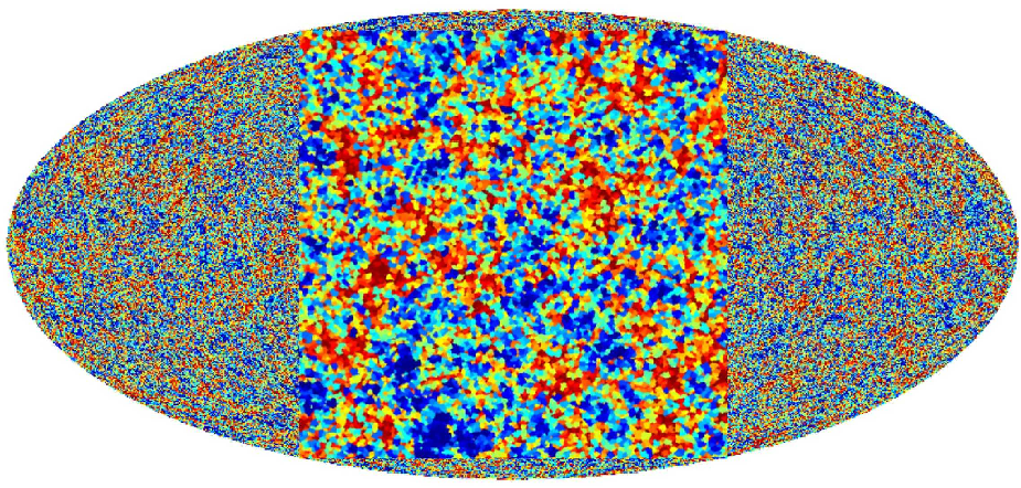
which is valid for sources at a single redshift , and is the adimensional comoving radial coordinate, hence . The detailed procedure to construct such maps from the simulation using equation (28) is described in Appendix D.1 (chosing the sampling strategy) and D.2 and in Teyssier et al. (2008). In practice, a set of degraded maps of was generated from the full resolution, down to in powers of 2, together with the corresponding masks (see Figure 5). Different levels of noise (corresponding to ) and maps with/without Galactic masks are considered. The corresponding simulations are labeled as . Cartesian maps are also used, labeled as corresponding to Cartesian sections of the full-sky maps, where for commodity, the experiments involving high resolution where calibrated. Here the flag refers to whether or not the non-linear model is accounted for.
3.2.3 Penalty weight
In this paper, the weight of the penalty, , in equation (24) is chosen so that the cutoff corresponds to the scale, at the intersection of the signal and the noise power spectra, see e.g. Figure 7. Specifically
In a more realistic situation, when the power spectrum of the signal is unknown, generalized cross validation could be used to find this scale. When penalty is implemented (see Section 2.1.4), the parameter entering equation (16) is chosen so that it cuts off the tail of the PDF of the Laplacian of the recovered field at the 3- level.
3.3 Optimization & Performance
Let us now turn to the optimization procedure and the performance of the algorithm.
3.3.1 Optimization
Recall that the procedure assumes here a sampling strategy, since the noisy field is given on a pixelisation of the sphere. To solve the optimization problem, we used the algorithm vmlm from OptimPack (Thiébaut, 2002) which only involves computing the objective function and its partial derivative with respect to the parameters . Vmlm is an unconstrained version of vmlmb which has been used for the deblurring problem and which is described in some details in section 2.1. The optimization of equation (24) is carried by computing in turn equation (18) and Equations (28) and (B.2) using Healpix (Górski & et al. (1999)) in OpenMP or MPI.
3.3.2 Overall Performance
Each back and forth transform takes respectively , , , , and seconds on an octo opteron for equal to , , , , and , see Table 1. The linearized problem without mask converges typically in a dozen iterations (which typically only involve a back and forth transform, unless the convergence is poor). The linearized mask problem takes a few hundred iterations, see Table 3, and so does the non-linear problem (or the linearized problem with a non-linear penalty function).
4 Validation and post analysis
Let us illustrate on a sequence of statistical tests several crucial features of the ASKI map making algorithm: its ability to fill gaps, its ability to preserve the geometry and sharpness of clusters and maintain the gravitational nature of the signal in the presence of masks, and the freedom to choose strong/weak prior on the two-points correlation. These properties are important in various contexts of the weak lensing studies, such as the estimation of cosmological parameters, the physics of clusters, the interpretation of tomographic data from upcoming surveys, constraining the dark energy equation of state through the redshift evolution of statistical and topological tracers. We chose a selection of statistical tests that are sensitive to different aspects of map-making.
4.1 One point statistics
4.1.1 Cluster counts

One of the main assets of high resolution full-sky lensing maps is to probe multiple scales: it then becomes possible to sample the non linear transition scale and, e.g. study the shape of clusters. Figure 9 illustrates this feature while displaying the result of the inversion with and penalties. For this experiment, a Cartesian subset at galactic coordinates was extracted. The corresponding non-linear shear field was generated via Fourier transform, and noised with a white additive noise of SNR of 1. This set was then inverted while assuming (bottom right) and (top right) penalties. The choice for the two penalty weights, and was made on the basis of least square residual in the inverted maps. The improvement of over penalty is significant. This statement is made more quantitative in Figure 10 which displays the PDF of the peaks within that image for the initial map (top left panel of Figure 9) computed following the peak patch prescription described in Section 4.3.1. The agreement between the input and the recovered distribution is significantly enhanced by the optimal (top right) penalty.

4.1.2 Skewness and Kurtosis


The simplest statistics to explore the non linear transition is the skewness, and the kurtosis, of the PDF of the recovered maps. Furthermore, it has been shown that these parameters provide a powerful tool to measure the underlying cosmological parameters (Bernardeau et al. (1997); Takada & Jain (2002); Takada & Jain (2004)). Figure 11 displays the evolution of these numbers as a function of scale in the initial and recovered maps, with and without galactic masking. The top hat filter used here is of width , while the harmonic number of each band is the mean of its boundary: . The recovery of skewness and kurtosis is good in the case of unmasked data. Of course it degrades with the scale as we reach . Using the reconstructed map is not the optimal way of measuring the 3 and 4 point functions at small scale. However, an optimal dedicated estimator can be built upon the same regularization technique. The masked case is not as good. There, a dedicated estimator, acting only on small, clean, pieces of the sky will probably yield better results.
4.1.3 Accounting for a non-linear model
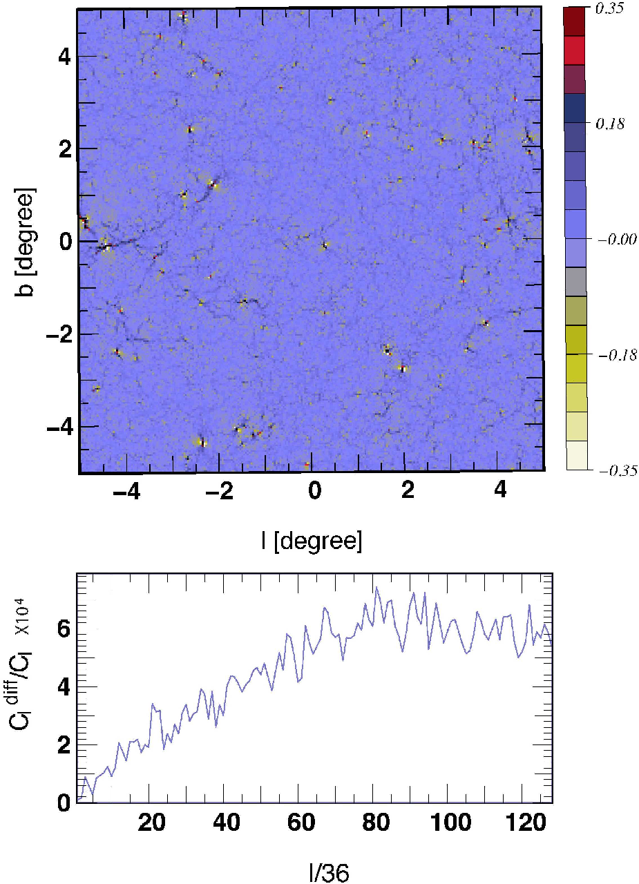
Figure 8 shows the effect of accounting for the non linearity in equation (17). Here a set of Cartesian simulations is used . This map represents (a 100 times) the difference between the recovered map while accounting for in equation (17) in the inversion, and the recovered map while neglecting this factor. The difference is small in amplitude, but shows as expected the strongest bias near the clusters and the filaments, where is largest. The bottom panel represents the corresponding relative power spectrum, as a function of . Again the larger discrepancy occurs at higher , corresponding to the sharp peaks at the positions of the clusters. Hence the non-linearity should be accounted for in the model if the shape of the cluster is an issue (see also White (2005); Dodelson & Zhang (2005); Shapiro (2009)). For all practical purposes, we have therefore demonstrated that at scales below solving the linearized problem is de facto equivalent to the general non-linear problem when is neglected at the denominator in equation (17).
4.2 Two points statistics
Since ASKI was constructed to provide the optimal map given the measured shear, we do not expect that it will yield the optimal estimator for non-linear functions of these maps, such as the powerspectrum, bispectrum etc.. Nevertheless it is of interest to compare the two point statistics of input and recovered maps, to see how Aski deals with masks and how it affects the occurrence of spurious B modes.
4.2.1 Optimal Wiener filtering
Throughout this paper the prior
(“Laplacian prior”) is used in equation (39).
Let us briefly investigate how a customized (Wiener) prior for
changes the reconstruction at small scales. Figure 12 shows
that the corresponding power
spectra of the reconstructed kappa maps, as expected, differ mostly for scales where the signal to
noise is smaller than one. However, when the smoothing (Laplacian) prior amplitude
(see equation 27) is tuned to minimize the
reconstruction error as in the figure, the power spectra of the
reconstructed maps for the two different priors (Laplacian and Wiener)
are quite similar.
It is interesting to note that the power of the reconstructed map with
the Wiener prior (light brown line in Figure 12)
is systematically biased low as compared to the input power
spectrum. This reflects the fact that an optimal (minimum variance) estimation of the
power spectrum is not equivalent to a power spectrum estimation
on an optimal (minimum variance) reconstructed map. However, in the
simple case where we have noisy data without masks, the bias of the
power spectrum of the minimum variance map reconstruction is known, it
is simply given by where is
the power spectrum of the underlying kappa map (without noise), and
is the noise power spectrum in “kappa” space, which is
given approximately in our case by , where
is the noise variance per pixel in the shear field, and
is the solid angle of a pixel.
In Figure 12,
the noise level is shown by the horizontal dark blue line. One can see
in particular in the figure, that when the model power spectrum
(without noise) crosses the noise power spectrum, the power spectrum
of the minimum variance map (golden line) is lower than that of the
model by a factor of , as expected from the considerations above,
even in the presence of masks.
Thus an approximate, but simple way to get an unbiased estimate of the
kappa power spectrum is to correct the minimum variance map power spectrum
by the ratio . Note however that a true
minimum variance power spectrum estimation of the kappa field is not the aim of the
present method (see e.g. Pen (2003) for the flat-sky case).

Nevertheless elsewhere in this paper, a smoothing prior which is not customized to the specific problem is preferred.
4.2.2 Filling gaps within masks
| 128 | 256 | 512 | 1024 | 2048 | |
|---|---|---|---|---|---|
| time for one step (s) | 0.121 | 0.121 | 0.502 | 1.88 | 8.53 |
| number of steps (s) | 252 | 313 | 315 | 377 | 325 |
| total time (s) | 40.1 | 50.3 | 200 | 989 | 3340 |


Let us first compare visually the recovered map to the input map. Figure 13 illustrates a feature of the penalized reconstruction: it interpolates quite well and provides means to fill the gaps corresponding to the galactic cuts. For a more quantitative comparison we also plot on this figure the ridges of both fields (using the skeleton, see below), which match very well up to the very edge of the mask. The smoothing penalty also induces a level of extrapolation, best seen in the residuals, see Figure 18. The masking (or more generally, non uniform weights, ) nevertheless biases the reconstructed map, as seen on Figure 11 and 14.

Note finally that when masks are accounted for, it is straightforward to correct for them when computing the powerspectrum as the harmonic transform of the autocorrelation, which in turn is derived by correcting for the autocorrelation of the masks: (see Szapudi et al. (2001); Hivon et al. (2002); Chon et al. (2004) for details). When seeking the three-point correlations one could also proceed accordingly, and divide by the three-point correlation of the mask. Indeed a three-point reduced correlation is simply one plus the excess probability of finding triplets, which in turn is computed by counting the number of found triplets and dividing by the expected number of such triplets given the shape of the mask (Chen & Szapudi (2005)). This also applies if the mask is grey.
4.2.3 Residual B modes
Let us investigate the effect of leaking of B modes with the following experiment: the noise in the transform of the B channel is boosted by some fixed amount over a map which has Galactic cuts. This corresponds to the case where the is significantly larger than the noise, yet uncorrelated with the mode, corresponding to e.g. a systematic bias in the ellipticity extraction for example. It is expected that, due to masks, this mode will leak in . An example of such leak, for modes as large or up to times larger than the noise, is shown in Figure 18. The power spectrum of the residuals in the corresponding map is computed while masking in the residual the exact regions corresponding to the cuts. When this boost is zero, (bottom curve in Figure 17) the power spectrum of these residuals is flat and corresponds to the noise powerspectrum. In contrast, the stronger the boost the larger the scale below which this power spectrum is colored. Note that it was checked that, as expected, these coherent residuals disappear completely if the galactic cuts are ignored. It would also be interesting to compare the distribution of the shape of dark matter in input/recovered clusters.
Finally, note that Appendix C.2 discusses briefly the effect of noise in powerspectrum estimation.
4.3 Alternative statistics: critical sets
Let us close this section with a quantitative comparison of the input and the recovered map using more exotic probes to estimate the quality of the reconstruction, and the prospect it offers for dark energy measurements. Indeed, the predictions of the perturbative hierarchical clustering model are often given through the hierarchy of the differences between the moments to their Gaussian limit. Yet higher order moments are generally difficult to test directly in real-life observations, due to their sensitivity to very rare events. As argued in Pogosyan et al. (2009) the geometrical analysis of the critical sets in the field (extrema counts, Genus, critical lines etc..) may provide more robust measures of non-Gaussianity, and is becoming elsewhere an active field of investigation (Gott et al., 2009; Park et al., 2005).
4.3.1 Peak patch counts and area


Even though many tools are available to identify peaks within the reconstructed map, let us validate here our reconstruction using a segmentation of both the initial and the recovered maps using peak patches on the sphere, which are a segmentation of the map based on the attraction patches of the map when following its gradient (see Sousbie et al. (2008)). Within each peak patch (see Figure 19), the brightest pixel is assigned a mass corresponding to the enclosed mass within the peak patch. This quantity is gravitationally motivated (as the patch corresponds to the attraction region of the cluster) and is both robust (as the geometry of the patch only depends on the imposed smoothing length, which in turn is fixed by the resolution of the survey) and sensitive to small features in the map; it is therefore a good indicator of the quality of the reconstruction. Figure 15 (left panel) displays the corresponding PDFs before and after reconstruction. As expected, the recovered point source PDF has a shifted mode and is less skewed than the original distribution. This trend decreases with increasing SNR. For realistic galaxy counts of 40 ngal arcmin, the agreement between the input and the recovered PDF is fairly good, and the corresponding residual bias can be modeled (as the reconstruction is essentially a smoothing of the underlying map). This could lead to interesting constraints on and when used in conjunction with weak lensing tomography in order to probe its redshift evolution. The right panel of Figure 15 focuses on a different quantity, the area of the patches, which when compared to the area of the corresponding void patches, could also be used as a measure of the gravitationally induced non gaussianities, together with their shape (higher moments of within a patch). Again, the reconstruction seems to recover this distribution well enough to suggest that such a tool could be used in the future to study the cosmic evolution of the projected web.
4.3.2 Topology & geometry: critical lines
Let us now compare the shape of the recovered map to the initial map from the point of view of its critical lines. For this purpose, let us use here the skeleton as a geometric probe (Novikov et al. (2006); Sousbie et al. (2007)). It is defined in 2D as the boundary of the void patches, which in turn are a segmentation of the map based on the valleys of the map (corresponding to the peak patches (defined above) of minus the field). The skeleton of the initial field and the recovered fields for simulation is computed, and represented in Figure 13. The recovered skeletons are qualitatively fairly close to the original skeleton, which demonstrates that the local topology and geometry of the field is well recovered. Let us make this comparison more quantitative. The differential length per unit area of the recovered field (the set with and as labeled)99 9 Note that ngal. over the initial map (thin line) as a function of density threshold is also shown in Figure 16, while Figure 6 shows the corresponding maps for similar runs, together with a map of the orientation of the field. The agreement increases at larger density thresholds, which suggests that the topology of dense regions is well recovered1010 10 In fact the relative distance between the recovered and the input skeleton could also be used as an alternative to the differential length see Caucci et al. (2008).. The total length was shown (Sousbie et al. (2008)) to trace well the underlying shape parameter of the powerspectrum and has been used in 3D to constaint the dark matter content of the universe (Sousbie et al. (2006)). As shown in Pogosyan et al. (2009) this would work for two dimensional maps and could therefore be used with maps such as those reconstructed via the present method. The redshift evolution of this differential count, when tomographic data is available, could complement e.g. Genus measurements as means of constraining the dark energy equation of state in a manner which could be more robust than direct cumulant estimation. Eventually, the skeleton could also be used to characterize the connectivity of clusters (i.e. the number of connected projected filaments), as it will also depend on the cosmic dark energy content of the universe (Pichon & al. (2009)).

This rapid review has shown that, depending on the final objective (cosmological parameters, cross correlation with other maps etc.), a variety of estimators can be extracted from the recovered maps. Aski was shown to perform rather well with respect to these estimators. Defining the best combination of these estimators, – and the optimal penalty associated – will be one of the key topic lensing research for the coming years.
5 Conclusion & Discussion
This paper sketched possible solutions to issues that a full-sky weak-lensing pipeline will have to address, and presented an inverse method implementing the debluring of the image and the map making step.
Weak lensing surveys require measuring statistical distributions of the morphological parameters (ellipticity, orientation, …) of a very large number of galaxies. This paper demonstrated that these parameters can be measured with a better accuracy and strongly reduced bias if the deep sky images are properly deblurred prior to the shape measurements. Using a relative figure of merit (the recovered SExtractor ellipticity) we have shown that this deblurring could in crowded fields improve more than tenfold the accuracy of the recovered ellipticities.

This deblurring is critical in crowded regions, where the overlapping of stars and galaxies otherwise prevents accurate morphological estimation. Henceforth dealing with such regions is important for a full-sky survey. Since such surveys will require the processing of a great number of large images, the calibration of these techniques is automated on the images themselves via cross validation after identification and removal of the stars within the field (see Figure 1). In particular the level of regularization, and the threshold are automatically tuned in order to deal with the noise level and the dynamics of the raw images. The gap-filling interpolation feature of the inversion would apply even more efficiently in this regime than in the map reconstruction regime described in Section 3. The algorithm described here scales well since it only relies on DFTs: hence it could be applied to very large images such as those produced by modern surveys. Aski uses the efficient variable metric limited memory algorithm OptimPack, which allows both optimizations to scale to high resolutions. The deblurring is implemented on Cartesian maps as large as pixels. Generalized cross validation was shown to yield a quantitative threshold in order to remove accurately the point sources within the field, hence imposing the optimal level of smoothing for the galaxies only. In this paper, the focus was put on blurred 8-meter ground-based observations, but the implementation for EUCLID-like space missions should be straightforward. The above described improvements could clearly be reproduced if alternative state of the art shear estimators were to be used (as compared by the SHear Testing Program).
This paper also demonstrated that optimization in the context of Maximum A Posteriori provided a consistent framework for the optimal reconstruction of maps on the sphere. The main asset of the Aski algorithm is that the penalty can be applied in model space, while the optimization iterates back and forth between data space and model space. This freedom allows it to deal simultaneously with masks (in data space) and edge preserving penalties. Providing maps is critical both in its own right, as it maps the dark matter distribution of our universe and gives access to the underlying powerspectrum at large scale. Such maps are also interesting when cross-correlated with other surveys (optical surveys, CMB maps, lensing reconstruction and distribution of SZ clusters from the Planck mission, redshift evolution of X-ray sources counts etc..) in order to explore the evolution of the large-scale structure, and in the case of the surveys mapping the baryonic matter, to better understand biasing as a function of scale. Finally, though not optimally, it can be used to compute second and higher order statistics, and noticeably the three-point statistics, the Genus, cluster counts or the skeleton, which may constrain more efficiently the dark energy equation of state, as they are less sensitive to rare events. It should be stressed once more that while the reconstructed maps yield biased estimates of the power-spectrum and higher order statistics, the technique described in this paper can be adapted to build dedicated optimal estimators for each of those observables.
Section 4 demonstrated the quality and limitations of the reconstruction using various statistical tools on a full-sky simulation of with resolutions of up to pixels thanks again to the efficiency of Optimpack. In particular, it identified point sources of the fields, analyzed their PDF and showed that penalty was critical at small scales. It also investigated the effect of leakage of modes when Galactic cuts are present. It presented a method to probe the topology and geometry of a field on the sphere, the peak patches and the skeleton, and applied it to compare the recovered field to the initial field. Such tools allow us to quantify the differences between the two maps and act as an efficient source segmentation algorithm. Indeed, the degeneracy between the cosmological parameters is for instance best lifted with cluster counts. They may also turn out to be of importance when probing the dark energy equation of state as they are less sensitive to rare events. The Cartesian dual formulation of aski was also implemented and may prove useful for surveys where sky coverage is sufficiently small.

In short, Aski accounts for the possible building blocks that a full-scale pipeline aiming at sampling the dark matter distribution over the whole sky should provide. Specifically it allows for (i) automatically deblurring very large images using non-parametric self-calibrated edge-preserving deconvolution with positivity; (ii) carrying the large non-linear inverse problem of reconstructing the convergence from the shear using equation (17): the back and forth iterations between model and data are consistent with constraints in both spaces, and allow for an accurate recovery of cluster profiles and shapes; (iii) non-uniform weighting and masking: consistent with realistic Galactic cuts (and bright stars masking) and non-uniform sampling of the different regions of the sky, dealing transparently with the issue of the boundary; (iv) edge-preserving penalty yielding quasi point-like cluster reconstruction. Finally (v) it introduced peak patches and the skeleton on the sphere, together with its statistics.
Possible improvements/investigation beyond the scope of this paper involve: (i) comparing the absolute gain in shear estimation using alternative tools to Sextractor (such as Massey et al. (2007)) with more realistics galactic shapes; (ii) deblurring the images with a variable PSF within the field; (iii) building optimal estimators for the power spectrum , or the asymmetry (a possible option would be to rely on perturbation theory, and invert the non-linear problem for both and ); (iv) inverting for and simultaneously and checking a posteriori the amplitude of the modes (an alternative to the model described in equation (19); the issue of unicity of the solution will be a challenge); (v) carrying the deprojection while assuming prior knowledge of a complete distribution of source planes in equation (28) (the corresponding inverse problem remains linear, with an effective kernel which depends on the optical configuration and the distribution of galaxies as a function of redshift); (vi) moving away from the Born approximation, which involves solving Poisson’s equation for each slice, and ray-tracing back to the source while solving for the lens equation though all the slices; (vii) implementing a more realistic noise modeling (which amounts to changing the cost function, equation (24)); (viii) studying the shape of dark matter distribution in clusters and groups: typically this would also involve cross-correlating the corresponding distribution with the light at various wavelengths, (ix) defining the post analysis which most sensitive to dark energy, given the feature of the surveys to come and finally (x) propagating the analysis up to the cosmic figure of merit for the dark energy parameters.
Acknowledgments
We thank Dmitry Pogosyan, Dominique Aubert, Eric Hivon, Martin Kilbinger and Yannick Mellier for comments and suggestions, the Horizon 4 team and the staff at the CCRT for their help in producing the simulation, and D. Munro for freely distributing his Yorick programming language and opengl interface (available at http://yorick.sourceforge.net/) The galactic mask was provided to us by Adam Amara. This work was carried within the framework of the horizon project: www.projet-horizon.fr.
References
- Abrial et al. (2008) Abrial P., Moudden Y., Starck J.-L., Fadili J., Delabrouille J., Nguyen M. K., 2008, Statistical Methodology, 5, 289
- Aubert et al. (2004) Aubert D., Pichon C., Colombi S., 2004, MNRAS, 352, 376
- Aubert & Kornprobst (2008) Aubert G., Kornprobst P., 2008, Mathematical Problems in Image Processing: Partial Differential Equations and the Calculus of Variations (Applied Mathematical Sciences), first edition edn. Springer Verlag
- Bartelmann et al. (1996) Bartelmann M., Narayan R., Seitz S., Schneider P., 1996, ApJ Let., 464, L115+
- Bartelmann & Schneider (2001) Bartelmann M., Schneider P., 2001, Phys. Rep., 340, 291
- Benabed & Scoccimarro (2005) Benabed K., Scoccimarro R., 2005, Arxiv preprint astro-ph
- Bernardeau et al. (2002) Bernardeau F., Mellier Y., van Waerbeke L., 2002, Arxiv preprint astro-ph
- Bernardeau et al. (1997) Bernardeau F., van Waerbeke L., Mellier Y., 1997, Astronomy and Astrophysics, 322, 1
- Bertin & Arnouts (1996) Bertin E., Arnouts S., 1996, aaps, 117, 393
- Bradac et al. (2005) Bradac M., Schneider P., Lombardi M., Erben T., 2005, arXiv, astro-ph
- Bridle & Abdalla (2007) Bridle S., Abdalla F., 2007, The Astrophysical Journal
- Bridle et al. (1998) Bridle S., Hobson M., Lasenby A., Saunders R., 1998, Mon. Not. R. Astron. Soc.
- Cacciato et al. (2006) Cacciato M., Bartelmann M., Meneghetti M., Moscardini L., 2006, arXiv, astro-ph
- Caucci et al. (2008) Caucci S., Colombi S., Pichon C., Rollinde E., Petitjean P., Sousbie T., 2008, MNRAS in press, pp 000–000
- Chen & Szapudi (2005) Chen G., Szapudi I., 2005, ApJ, 635, 743
- Chon et al. (2004) Chon G., Challinor A., Prunet S., Hivon E., Szapudi I., 2004, MNRAS, 350, 914
- Crittenden et al. (2002) Crittenden R., Natarajan P., Pen U., Theuns T., 2002, The Astrophysical Journal
- Dodelson & Zhang (2005) Dodelson S., Zhang P., 2005, Phys. Rev. D, 72, 083001
- Erben et al. (2001) Erben T., Van Waerbeke L., Bertin E., Mellier Y., Schneider P., 2001, AAP , 366, 717
- Fu & et al. (2008) Fu et al. 2008, Astronomy & Astrophysics
- Girard (1989) Girard D. A., 1989, Numr. Math., 56, 1
- Golub et al. (1979) Golub G. H., Heath M., Wahba G., 1979, Technometrics, 21, 215
- Górski & et al. (1999) Górski K. M., et al. 1999, in Banday A. J., Sheth R. K., da Costa L. N., eds, Evolution of Large Scale Structure : From Recombination to Garching Analysis issues for large CMB data sets. pp 37–+
- Gott et al. (2009) Gott J. R., Choi Y.-Y., Park C., Kim J., 2009, ApJ Let., 695, L45
- Halkola et al. (2006) Halkola A., Seitz S., Pannella M., 2006, arXiv, astro-ph
- Heymans (2006) Heymans e. a., 2006, MNRAS, 368, 1323
- Hirata & Seljak (2004) Hirata C., Seljak U., 2004, Physical Review D
- Hivon et al. (2002) Hivon E., Górski K. M., Netterfield C. B., Crill B. P., Prunet S., Hansen F., 2002, ApJ, 567, 2
- Högbom (1974) Högbom J. A., 1974, A&AS , 15, 417
- Hu (2000) Hu W., 2000, Phys. Rev. D, 62, 043007
- Jee et al. (2007) Jee M., Ford H., Illingworh G., White R., et al. 2007, The Astrophysical Journal
- Kilbinger & Schneider (2005) Kilbinger M., Schneider P., 2005, Arxiv preprint astro-ph
- Kitching et al. (2006) Kitching T., Heavens A., Taylor A., Brown M., et al. 2006, Arxiv preprint astro-ph
- Marshall et al. (2002) Marshall P., Hobson M., Gull S., Bridle S., 2002, Monthly Notices of the Royal Astronomical Society
- Massey (2007) Massey e. a., 2007, MNRAS, 376, 13
- Massey et al. (2007) Massey R., Rhodes J., Leauthaud A., Capak P., Ellis R., et al. 2007, Arxiv preprint astro-ph
- Mugnier et al. (2004) Mugnier L. M., Fusco T., Conan J.-M., 2004, 21, 1841
- Nocedal & Wright (2006) Nocedal J., Wright S. J., 2006, Numerical Optimization, second edition edn. Springer Verlag
- Novikov et al. (2006) Novikov D., Colombi S., Doré O., 2006, MNRAS, 366, 1201
- Park et al. (2005) Park C., Choi Y.-Y., Vogeley M. S., Gott J. R. I., Kim J., Hikage C., Matsubara T., Park M.-G., Suto Y., Weinberg D. H., 2005, ApJ, 633, 11
- Pen (2003) Pen U.-L., 2003, MNRAS, 346, 619
- Pichon & al. (2009) Pichon C., al. 2009, MNRAS in prep., pp 000–000
- Pichon & Bernardeau (1999) Pichon C., Bernardeau F., 1999, Astronomy and Astrophysics, 343, 663
- Pichon & Thiébaut (1998) Pichon C., Thiébaut E., 1998, MNRAS, 301, 419
- Pichon et al. (2001) Pichon C., Vergely J. L., Rollinde E., Colombi S., Petitjean P., 2001, MNRAS, 326, 597
- Pires et al. (2008) Pires S., Starck J. ., Amara A., Teyssier R., Refregier A., Fadili J., 2008, ArXiv e-prints
- Pogosyan et al. (2009) Pogosyan D., Gay C., Pichon C., 2009, ArXiv e-prints
- Pogosyan et al. (2009) Pogosyan D., Pichon C., Gay C., Prunet S., Cardoso J. F., Sousbie T., Colombi S., 2009, MNRAS, 396, 635
- Prunet et al. (2008) Prunet S., Pichon C., Aubert D., Pogosyan D., Teyssier R., Gottloeber S., 2008, ApJ Sup., 178, 179
- Richardson (1972) Richardson W. H., 1972, Journal of the Optical Society of America (1917-1983), 62, 55
- Schirmer et al. (2007) Schirmer M., Erben T., Hetterscheidt M., Schneider P., 2007, Astronomy & Astrophysics, 462
- Schneider et al. (2002) Schneider P., van Waerbeke L., Kilbinger M., Mellier Y., 2002, AAP , 396, 1
- Schwarz (1978) Schwarz U. J., 1978, AAP , 65, 345
- Seitz et al. (1998) Seitz S., Schneider P., Bartelmann M., 1998, AAP , 337, 325
- Seitz et al. (1998) Seitz S., Schneider P., Bartelmann M., 1998, Arxiv preprint astro-ph
- Shapiro (2009) Shapiro C., 2009, ApJ, 696, 775
- Sheth & Tormen (1999) Sheth R. K., Tormen G., 1999, MNRAS, 308, 119
- Skilling et al. (1979) Skilling J., Strong A. W., Bennett K., 1979, MNRAS, 187, 145
- Soulez et al. (2007) Soulez F., Denis L., Thiébaut E., Fournier C., Goepfert C., 2007, J. Opt. Soc. Am. A, 24, 3708
- Sousbie et al. (2008) Sousbie T., Pichon C., Colombi 2008, MNRAS , pp 000–000
- Sousbie et al. (2007) Sousbie T., Pichon C., Colombi S., Novikov D., Pogosyan D., 2007, ArXiv e-prints, 707
- Sousbie et al. (2006) Sousbie T., Pichon C., Courtois H., Colombi S., Novikov D., 2006, ArXiv Astrophysics e-prints
- Starck et al. (2005) Starck J., Pires S., Refregier A., 2005, Arxiv preprint astro-ph
- Szapudi et al. (2001) Szapudi I., Prunet S., Colombi S., 2001, ApJ Let., 561, L11
- Takada & Jain (2002) Takada M., Jain B., 2002, Monthly Notice of the Royal Astronomical Society, 337, 875
- Takada & Jain (2003) Takada M., Jain B., 2003, Monthly Notices of the Royal Astronomical Society
- Takada & Jain (2004) Takada M., Jain B., 2004, Monthly Notices of the Royal Astronomical Society, 348, 897
- Tarantola & Valette (1982) Tarantola A., Valette B., 1982, Reviews of Geophysics and Space Physics, 20, 219
- Teyssier (2002) Teyssier R., 2002, AAP , 385, 337
- Teyssier et al. (2008) Teyssier R., Pires S., Prunet S., Aubert D., Pichon C., Amara A., Benabed K., Colombi S., Refregier A., Starck J.-L., 2008, ArXiv e-prints
- Thiébaut (2002) Thiébaut E., 2002, in Starck J.-L., Murtagh F. D., eds, Astronomical Data Analysis II Vol. 4847, Optimization issues in blind deconvolution algorithms. pp 174–183
- Thiébaut (2005) Thiébaut E., 2005, in Foy R., Foy F. C., eds, NATO ASIB Proc. 198: Optics in astrophysics Introduction to Image Reconstruction and Inverse Problems. pp 397–+
- van Waerbeke et al. (1999) van Waerbeke L., Bernardeau F., Mellier Y., 1999, AAP , 342, 15
- Wahba (1990) Wahba G., ed. 1990, Spline models for observational data
- White (2005) White M., 2005, Astroparticle Physics, 23, 349
Appendix A Efficient Star Removal
We have observed that for realistic deep field images, generalized cross validation (GCV) yields an hyper-parameter value which is relevant to regularize the higher part of the dynamic (mainly due to stars, i.e. point-like objects which concentrate their luminous energy in a very small area) but which is much too low to regularize the lower parts ot the dynamic where galaxies remain. Indeed, when dealing with images with a large dynamical range, GCV yields a value of the regularization level which is necessarily a compromise between not smoothing too much the sharp features and sufficient smoothing of low contrasted structures to avoid noise amplification. The solution to the problem of underestimating the regularization weight can be solved by applying the GCV method onto the image with no stars. We want to find structures of known shape but unknown position and intensity in the image . In our case, is the PSF since we want to detect stars. This reasoning could however be generalized to other kind of objects. If a single object of this shape is present in the image, this could be achieved by considering the objective function:
to be minimized w.r.t. the weight and the offset , here a 2-D vector. In fact, since may be crowded with similar structures (or with other fainter structures), a better strategy is to limit the local fit to a small region of interest (ROI) around the structure. This is achieved by minimizing:
where is equal to 1 within the region of interest (ROI) and equal to 0 outside the ROI. Minimization of w.r.t. yields the best intensity for a local fit around :
Inserting in the objective function yields:
Since , by defining , the local criterion and local best intensity can be rewritten as:
These parameters can be computed for all shifts by an integer number of pixels by means of FFT’s (cross-correlation product). Unfortunately, the overall minimum of is not the best choice for removing the brightest structures since there is no warranty that this minimum corresponds to a bright object. It is better to select the the location which yields the brightest structure, i.e. the maximum of . After removal of the contribution from the data, this technique can be repeated to detect the second brightest source, and so on. The corresponding algorithm is very similar to the clean method (Högbom, 1974; Schwarz, 1978) with the further refinement of accounting for non-stationary noise and missing data. It has been shown that it achieves sub-pixel precision (Soulez et al., 2007) and that it could be used to detect (and remove) out of field sources (Soulez et al., 2007).
Appendix B Model on the sphere
Let us describe in more details the model used for the inversion of Section 3.1.
B.1 Discretization and Sampling
After discretization and using explicit indices, the model in equation (17) writes:
where the index runs over the sky coordinates , index corresponds to the two components and of the polarization, whereas and are the harmonic indices and refers to the two components of the spinned 2-harmonic. In words, the discretization yields:
Here the fields and are linear functions of the complex field of the spherical harmonic coefficients of . Using the matrix notation of the paper, and write:
where and ; with explicit index notations:
and
To get the detailed expression of the operator we start from the relationship between the lensing potential, the convergence and the shear fields on the sphere. To do this, we need first to define the null diad, based on the polar coordinates unit vectors:
| (29) |
Given this diad, the lensing potential, convergence and shear are related through:
where is the spherical metric tensor, and the spherical covariant derivative. Now, using the following expression of the second covariant derivative of a scalar spherical harmonic:
we can relate the convergence and shear fields to the spherical harmonic coefficients of the lensing potential:
| (30) | |||||
| (31) | |||||
| (32) |
where the last equality defines the and modes coefficients. Relating the latter coefficients to the spherical harmonics decomposition of written above, we get the following expression for the operator coefficients:
| (33) | |||||
| (34) |
where are the spherical harmonics coefficients of the convergence field.
B.2 Likelihood
The data related term in the cost function is
The gradient of this term is needed to find the solution of the inverse problem:
where
are the weighted residuals, and where
| (35) |
B.3 Regularization
The aim of the regularization is to avoid ill-conditioning and noise amplification in the inversion. Following a Bayesian prescription, this can be achieved by requiring the field to obey some known a priori statistics, or while assuming a roughness penalty for .
B.3.1 Wiener filter and penalty
Assuming the field has Gaussian distribution with mean and covariance , the prior penalty should write:
For a field with zero mean () and stationary isotropic statistics, the regularization can be expressed in terms of the harmonic coefficients:
| (36) |
with
| (37) |
where the angular brackets denote here the expected value taken over the index of the harmonic coefficients. The gradient of the stationnary isotropic Gaussian regularization in equation (36) is:
Note that the regularization in equation (36) with a known power spectrum for the field yields the so-called Wiener filter.
When the power spectrum of is not exactly known, a quadratic prior can alternatively be used. For instance:
| (38) |
In our framework, effective regularization is achieved by requiring the field to be somewhat smooth. In practice, this is obtained by requiring to be a positive non-decreasing function of the index . Note that, from a Bayesian viewpoint, the regularization in equation (38) corresponds to the prior that is a stationary isotropic centered Gaussian field with mean power spectrum , which is similar to the Wiener filter except that the exact statistics is not known in advance (because some parameters of the regularization have to be tuned; for instance, need not be equal to one). The gradient of in equation (38) reads:
The quadratic prior in equation (38) can be expressed in terms of :
where is some finite difference operator which gives an estimate of the local fluctuation of the field, and is the (pseudo-)inverse of the scalar spherical harmonics matrix. In our framework, we choose to measure the amplitude of the local fluctuations of the field by its Laplacian and to express the regularization penalty as:
| (39) |
where the cost function is an increasing function of . When , our regulariztion is a quadratic penalty similar to equation (38). Using matrix notation, the Laplacian of the field write :
where . In order to perform the minimization, the gradient of the regularization must be computed. By the chain rule:
| (40) | |||||
where is the derivative of .
B.3.2 penalty
As for the image restoration, quadratic regularization yields spuriours ripples in the regularized map. To avoid them, we propose to use a cost function applied to the Laplacian of . The details of the cost function are discussed in section 2.1.4.Taking , with given in equation (16), yields:
In practice, we use GCV to set the level of the regularization, possibly after cluster removal (as explained in Appendix A) and the threshold is set to be where and is the standard deviation of the histogram of spatial finite differences.
Appendix C From the sphere to the plane
In section 3.1.2 we sketched the correspondence between the fullsky and the flat sky approximation of the lens equation. Let us derive it here precisely and use it to investigate the effect of shot noise in the estimation of .
C.1 Derivation
Following closely Hu (2000), let us start with a scalar field on the sphere, and its decomposition on the usual spherical harmonics:
| (41) |
and let us define
| (42) |
together with the inverse relation
where is the polar angle of the vector in Fourier space. Let us show that corresponds to the Fourier decomposition of the field in the flat-sky limit (small angles near the pole). Indeed, taking the asymptotic behavior of the spherical harmonics
together with the plane-wave expansion in terms of Bessel functions
We get from equation (41)
For a spin-2 field, let us proceed likewise. We start from the all-sky definition of a spin-2 tensor field, and its decomposition in spin-2 spherical harmonics:
| (43) |
where is defined in the spherical tangent coordinates . We define, as in equation (42), the Fourier modes of the components of the spin-2 field as . We have in the flat-sky limit the following asymptotic form for the spin-2 spherical harmonics:
| (44) |
Plugging equation (43) into equation (44) yields:
Redefining the spin-2 field in the fixed coordinate system such that the first axis () is aligned with , we obtain:
| (45) |
where . Expanding , we can relate these rotationally invariant quantities to the Fourier transforms of the spin-2 field individual components. In the case of weak lensing, we get the following flat sky limits:
| (46) | |||||
| (47) |
After identification, we thus get the limits for the operator :
| (48) |
independently of the Fourier mode modulus.
C.2 SNR investigation in the plane

Let us briefly investigate the effect of noise on the recovery of the powerspectrum arising from the finite number of sources per unit area. For this purpose, let us consider the simplest setting corresponding to a cartesian map without mask which can therefore be inverted linearly following equations (22)-(23). In this regime, the regularized solution is simply given in Fourier space by
| (49) |
where , and are the Fourier transform of the observed shear and convergence, and the penalty hyperparameter. In Figure 20 we make use of the simulation , whose residues (after non linear inversion) are shown in Figure (8). Here 50 Monte Carlo realizations of the noise corresponding 40 galaxies/arcmin are averaged to produce an estimate of the corresponding errors. Clearly the shot noise remains small at all considered frequencies.cpp
Appendix D Convergence maps
The inversion technique described in the main text was validated using the mocks extracted from the horizon-4 simulation (Prunet et al., 2008). Let us briefly describe here how this simulation was used to generate mock slices and maps.
D.1 Light cone generation

The generation of a light cone during run time can be performed easily at each coarse time step of the simulation. Given a choice of the observer position in the simulation box, that we suppose here for simplicity to be at the origin of coordinates, it is easy to select the particles that belong to the slice in between redshifts corresponding to two successive coarse time steps: if are the comoving coordinates of a particle, and its comoving distance from the observer, we must have for the particle to be selected, where is the comoving distance that a photon covers between redshift and present time in the simulation box: , where is the speed of light and the expansion factor. The problem is that structures evolve during a coarse time step, so there are necessarily some discontinuities at the border between two successive light cone slices. These discontinuities are due to large scale motions of particles plus their thermal velocity within dark matter halos. Given the large size of the simulation considered here, thermal motion within the largest cluster are expect to bring the most significant effects of discontinuity. For a particle with peculiar velocity , the largest discontinuity to be expected, i.e. the largest possible difference between expected and actual position of the particle is given by
| (50) |
In equation (50), we performed a linear Lagrangian approximation, i.e. we neglected variations of the velocity of the particle during the coarse time step. Using Press & Schechter formalism, or the improved formula of Sheth & Tormen (1999), the mass of the largest cluster in the Horizon simulation solves approximately the implicit equation
| (51) |
where is the critical density of the Universe and is the fraction of mass in the Universe in objects of mass larger than . Basically, this equation states that the mass in objects of mass larger than is equal to , which means that we are left with only one cluster of mass , the largest detectable cluster in our cube of size . We can compute with the usual formula, e.g.
| (52) |
with where is the linear variance at redshift corresponding to mass scale , and is given by equation (10) of Sheth & Tormen (1999). Performing these calculations, we find that the largest cluster at present time in a cube of size Mpc should have a typical mass of . With a standard Friend-of-friend algorithm using a linking parameter , we find that the most massive halo detected in the simulation presents a somewhat larger mass, . Yet, in that rare events regime, we cannot expect our theoretical estimate to be more accurate. What matters, though, is the thermal velocity rather than the mass. Applying the Virial theorem, we have (e.g., Peacock, 1999) with
where is the density parameter as a function of redshift (). These expressions are given in physical coordinates hence the factor in the expression of . This reads, at , km/s for . In the largest cluster of the simulation, the overall velocity dispersion is of the order of km/s, a slightly larger value that reflects the actual value of the mass. To be conservative, we estimate the expected errors in equation (50) with the Virial velocity rescaled by a factor , and with a further multiplication by a factor 3 to be in the 3 regime. The corresponding maximal expected discontinuity displacement is shown in Mpc as a function of the expansion factor on Figure 21. As expected from the dynamically self-consistent calculation of the coarse time step (which is basically determined by a Courant condition using the velocity field), the comoving error does not change significantly with redshift and remains below the very conservative limit of 200 kpc. Obviously, we expect in practice the errors brought by discontinuities to be in general much smaller than that, as for the present errors corresponds to unrealistic velocities as large as about 6000 km/s!
D.2 From slices to maps
In the main text, the expression for as a function of the density contrast in the simulation is given in equation (28) in the geometric optic approximation. Let us rearrange this formula in a form that is more suited to integration over redshift slices in a simulation.
where
is a slice-related weight, and the integral over the density contrast, , reads
where
is the comoving surface of the spherical pixel. Putting all together, we get the following formula for the convergence map:
Once the map is available it is straightforward to build the corresponding using equation (17).