Theory of superconducting and magnetic proximity effect in SF structures with inhomogeneous magnetization textures and spin-active interfaces
Abstract
We present a study of the proximity effect and the inverse proximity effect in a superconductorferromagnet bilayer, taking into account several important factors which mostly have been ignored in the literature so far. These include spin-dependent interfacial phase shifts (spin-DIPS) and inhomogeneous textures of the magnetization in the ferromagnetic layer, both of which are expected to be present in real experimental samples. Our approach is numerical, allowing us to access the full proximity effect regime. In Part I of this work, we study the superconducting proximity effect and the resulting local density of states in an inhomogeneous ferromagnet with a non-trivial magnetic texture. Our two main results in Part I are a study of how Bloch and Néel domain walls affect the proximity-induced superconducting correlations and a study of the superconducting proximity effect in a conical ferromagnet. The latter topic should be relevant for the ferromagnet Ho, which was recently used in an experiment to demonstrate the possibility to generate and sustain long-range triplet superconducting correlations. In Part II of this work, we investigate the inverse proximity effect with emphasis on the induced magnetization in the superconducting region as a result of the ”leakage” from the ferromagnetic region. It is shown that the presence of spin-DIPS modify conclusions obtained previously in the literature with regard to the induced magnetization in the superconducting region. In particular, we find that the spin-DIPS can trigger an anti-screening effect of the magnetization, leading to an induced magnetization in the superconducting region with the same sign as in the proximity ferromagnet.
pacs
74.20.Rp, 74.50.+r, 74.20.-zI Introduction
The interplay between ferromagnetism and superconductivity has over the past decade attracted much interest from the condensed-matter physics community. Research on superconductorferromagnet (SF) heterostructures continues to benefit from great interest, which is fueled by the exciting phenomena arising from a fundamental physics point of view in addition to the prospect of harvesting functional devices in low-temperature nanotechnology.
There is currently intense activity in this particular research area (see e.g. Refs. 1, 2 and references therein). The interest in SF hybrid structures was boosted at the beginning of this millenium, primarily due to the theoretical proposition of proximity-induced odd-frequency correlations [3] and the experimental observation of 0- oscillations in SFS Josephson junctions. [4] A large amount of work has been devoted to odd-frequency pairing (see e.g. [5, 6, 7, 8, 9, 10, 11, 12, 13, 14, 15, 16, 17, 18, 19, 20, 21]) and the physics of 0- oscillations (see e.g. [22, 23, 24, 25, 26, 27, 28, 29, 30, 31, 32, 33, 34, 35, 36, 37, 38]) in SF heterostructures. The concept of odd-frequency pairing dates back to Refs. [39, 40, 41, 42] and was recently re-examined in Ref. [43].
So far, the proximity effect has received much more attention than the inverse proximity effect. In SF bilayers, the proximity effect causes superconducting correlations to penetrate into the ferromagnetic region [1]. Similarly, the inverse proximity effect induces ferromagnetic correlations in the superconducting region near the interface region.[44, 45, 46, 47] Often, the bulk solution is employed in the superconducting region, such that both the induced magnetic correlations and the self-consistency of the superconducting order parameter are neglected. However, it was shown in Ref. [62] that the induction of an odd-frequency triplet component would lead to a finite magnetization in the superconducting region close to the SF interface. Prior to this finding, some experimental groups had reported findings which pointed towards precisely such a phenomenon [64, 65]. Very recently, Xia et al.[63] presented an experimental observation of the inverse proximity effect in Al/(Co-Pd) and Pd/Ni bilayers by measuring the magneto-optical Kerr effect. Their data could be roughly fitted to the predictions of Ref. [62], and other experiments [44, 45, 64, 65, 66] have also addressed aspects of the inverse proximity effect SF bilayers.
In Ref. [67], the authors investigated the proximity-induced magnetization in the superconducting region of a SF bilayer, and found that the magnetization would oscillate in the clean limit (see also Ref. [68]) and decay monotonously in the diffusive limit, with a sign opposite to the magnetization in the bulk of the ferromagnet. The reason for this screening behavior in the superconductor was attributed to a scenario in which the spin- electron of a Cooper pair near the interface would prefer to be located in the ferromagnetic region, while its spin- partner would remain in the superconducting region, thus creating a magnetization with an opposite sign compared to the ferromagnet. By considering the weak proximity effect regime in the diffusive limit, both Ref. [62] and Ref. [67] arrived at this conclusion. However, it would be desirable to go beyond the approximation of a weak proximity effect employed in previous work to investigate if this may alter how the induced magnetization in the superconducting region behaves.
Moreover, none of the above works on the inverse proximity effect have properly included an important property which is intrinsic to SF interfaces, namely the spin-dependent interfacial phase shifts (spin-DIPS) that occur at the interface. The spin-DIPS have been shown to exert an important influence on various experimentally observable quantities in SF bilayers [28, 48, 69], and should be taken into account. For instance, the anomalous double peak structure in the local density of states (LDOS) in a diffusive SF bilayer reported very recently by SanGiorgio et al.in Ref. [50] was reproduced theoretically in Ref. [49] by using a numerical solution of the Usadel equation when including the effect of the spin-DIPS.
So far, due to the complexity of the problem, several assumptions have been usually made when treating SF hybrid structures. For instance, since the quasiclassical equations become quite complicated for inhomogeneous ferromagnets, they have been linearized in most of the previous works. However, presently, the direction of this research field tends towards a more realistic description of SF structures than the simplified models that mostly have been employed up to now. It is obvious that this is a necessary step in order to reconcile the theoretical predictions with experimentally observed data.
Our motivation for this work is to examine the effect of inhomogeneous magnetization textures and spin-DIPS on both the proximity effect and the inverse proximity effect in SF bilayers. This is directly relevant to two recent experimental studies [57, 63] which studied the superconducting proximity effect in the conical ferromagnet Ho and the inverse proximity effect in the superconducting region of a SF bilayer, respectively. As we shall show in this work, non-trivial magnetization textures and spin-DIPS have profound influence on the physical properties of SF bilayers, suggesting that their role must be taken seriously.
We divide this work into two parts which are devoted to the proximity effect in the ferromagnetic region (Part I) and the inverse proximity effect in the superconducting region (Part II). In Part I, we present results where we treat the role of magnetic properties at the interface and the possibility of inhomogeneous magnetization thoroughly. We study the proximity-induced density of states (DOS) in a SF bilayer which takes into account the presence of spin-DIPS at the interface and also the possibility of having a non-trivial magnetization texture (such as a domain wall) in the ferromagnetic region. In order to access the full proximity effect regime, we do not restrict ourselves to any limiting cases. Rather, we employ a full numerical solution of the DOS by means of the quasiclassical theory of superconductivity. We apply our theory to two cases of ferromagnets with an inhomogeneous magnetic texture, namely on one hand ferromagnets with domain walls and on the other hand conical ferromagnets.
In Part II, we study numerically and self-consistently the inverse proximity effect in a SF bilayer of finite size upon taking properly into account the spin-DIPS that occur at the SF interface. Our main objective is to study the influence exerted on the inverse proximity effect by the spin-DIPS. Surprisingly, we find that the spin-DIPS may invert the sign of the proximity-induced magnetization in the superconducting layer compared to the predictions of Refs. [62, 67]. Consequently, the spin-DIPS can trigger an anti-screening effect of the magnetization, which suggests that their role must be taken seriously in any attempt to construct a theory for the inverse proximity effect in SF bilayers. We also explain the basic mechanism behind the sign-inversion induced by the spin-DIPS.
This paper is organized as follows. In Section II.1, we present the theoretical framework we use to perform our computations in Part I, namely the quasiclassical theory of superconductivity in the diffusive limit for an inhomogeneous ferromagnet using the Ricatti parametrization. In Section II.2, we present our numerical results for proximity-effect and the local density of states for the two cases of ferromagnets with domain walls and with conical magnetic textures. In Section II.3, we present a discussion of our results obtained in Part I. Moving on to Part II of this work, we introduce a slightly different notation and parametrization for the Green’s function in Sec. III.1, which is easier to implement for a homogeneous SF bilayer. In Sec. III.2, we present our results for the inverse proximity effect, manifested through an induced magnetization in the superconducting region and in particular how it is influenced by the presence of spin-DIPS. The results for Part II are discussed in Sec. III.3, and we conclude with final remarks in Sec. IV. Throughout the paper, we will use boldface notation for 3-vectors, for matrices, and for matrices.
II Proximity effect in a SF bilayer with an inhomogeneous magnetization texture
II.1 Theoretical framework
In the first part of our work, we shall consider the proximity effect in the ferromagnetic region of an SF bilayer when the magnetization texture is inhomogeneous. This is the case e.g. in the presence of a domain-wall structure or conical ferromagnetism, which both will be treated below. We will use the quasiclassical theory of superconductivity [51], and consider the diffusive limit described by the Usadel equation [52].
II.1.1 Quasiclassical theory and Green’s functions
To account for an inhomogeneous magnetization in the ferromagnet, it is convenient to parametrize the Green’s function to obtain a simpler set of equations to solve. One possibility is to use a generalized -parametrization [53], as follows
| (1) |
where are the identity and Pauli matrices, and
| (2) |
Also, and . The Green’s function is then completely determined by the complex functions , , and with the additional constraint in order to satisfy .
However, for our purpose we find it both more convenient and elegant to use a Ricatti-parametrization of the Green’s function as follows [54, 55], as follows
| (3) |
This parametrization facilitates the numerical computations, and also ensures that . The unknown functions and are key elements in this parametrization of the Green’s function, and will be solved for below. Here, denotes a matrix and
| (4) |
In order to calculate the Green’s function , we need to solve the Usadel equation with appropriate boundary conditions at and . The two natural length scales associated with each of the long-range orders are the superconducting and ferromagnetic coherence lengths
| (5) |
where and denote the bulk values of the gap and the exchange field. We set for simplicity. The Usadel equation reads
| (6) |
and is supplemented with the boundary conditions [28, 48]
| (7) |
at where the interface is spin polarized along the z-axis, and at . Here, and we define
| (8) |
as the ratio between the resistance of the barrier region and the resistance in the ferromagnetic film (note that ). The barrier conductance is given by [28]
| (9) |
where and is the transmission coefficient for channel . The boundary conditions Eqs. (22) and (23) are derived under the assumption that , but this does not necessarily mean that the barrier conductance is small since there may be a large total number of channels through which transport may take place. The parameter describes the spin-DIPS taking place at the F side of the interface.[56] Since its exact value depend on the microscopic properties of the barrier region, they are here treated phenomenologically. We finally underline that the boundary conditions above are valid for planar diffusive contacts.
Since we employ a numerical solution, we have access to study the full proximity effect regime and also an, in principle, arbitrary spatial modulation of the exchange field. This is desirable in order to clarify effects associated with non-uniform ferromagnets, such as spiral magnetic ordering or the presence of domain walls. Inserting Eq. (3) into Eq. (21), we obtain the transport equation for the unknown function (and hence )
| (10) |
with . The boundary condition at reads
| (11) |
while at . For , we obtain
| (12) |
with the corresponding boundary condition
| (13) |
We have defined . Note that we use the bulk solution in the superconducting region, which is a good approximation when assuming that the superconducting region is much less disordered than the ferromagnet and when the interface transparency is small, as considered here (see detailed discussion in Sec. II.3). One finds that
| (14) |
The normalized DOS is finally evaluated by
| (15) |
In what follows, we will omit the effect of spin-flip and spin-orbit scattering to reduce the number of parameters in the problem. In comparison with real experimental data, however, the effects of these pair-breaking mechanisms are easily included in our framework by adding two terms and in Eq. (21) (see e.g. Ref. [20] for a detailed treatment). In this paper, we will focus on the role of the phase-shifts obtained at the interface due to the spin-split bands and the inhomogeneity of the exchange field in the ferromagnet.

II.1.2 Inhomogeneous magnetization
We will consider three types of inhomogeneous magnetic structures: Bloch walls, Néel walls, and conical ferromagnets (see Fig. 1). An example of the latter is the rare-earth heavy fermion elemental magnet Ho, although we hasten to add that while Ho features strong ferromagnet, we will consider the weakly ferromanetic case. These structures are shown in Fig. 1 and are to be contrasted with the usual assumption of a homogeneous exchange field in the ferromagnetic region. For the first two cases, the domain wall has a width and is taken to be located at the center of the ferromagnetic region . The Bloch wall is thus modelled by
| (16) |
while for the Néel wall. Here, we have defined
| (17) |
similarly to Ref. [55].
In the case of a conical ferromagnet, cf. Fig. 1, the magnetic moment belongs to a cone. In Ho, the opening angle is and the magnetic moment then rotates like a helix along the -axis with a turning angle per interatomic layer with distance (see Ref. [57] for a further discussion). Above 21 K, the conical ferromagnetic structure transforms into a spiral antiferromagnetic structure. Instead of using an abrupt change in the magnetization direction at each interatomic layer, we will model this transition smoothly since the effective field felt between the layers probably should be a weighed superposition of the exchange fields from the two closest layers. In the ferromagnetic phase, the spatial variation of the exchange field may thus be written as
| (18) |
II.2 Results
In what follows, we will choose the parameters of our model, corresponding to a realistic experimental setup in order to make our study directly relevant for experiments on SF bilayers. The numerical treatment makes use of built-in routines in MATLAB for a two-point boundary value problem for an ordinary differential equation. More specifically, we use a finite difference code which implements a three-stage Lobatto-Illa formula. An initial guess for the Ricatti-matrices is supplied with fixed boundary conditions, and the Usadel equation is then solved in the entire ferromagnetic region.
In the first part of this section, we will study the effect of domain walls in weak ferromagnets. Weak ferromagnetic alloys such as PdNi or CuNi are commonly employed in experiments, and the corresponding exchange field depends on the concentration of Ni, reaching up to tens of meV. The modification of the DOS is most dramatic in the case when the energy scales for the superconductivity and the ferromagnetism are of the same order, . This scenario appears to have been realized in Ref. 4 where Cu1-xNix with was used. The diffusion constant in the weakly ferromagnetic alloys is usually of order m2/s. The superconducting region is considered to act as a reservoir with thickness , while we fix the thickness of the ferromagnetic region at . This typically corresponds to a thickness of the ferromagnetic layer 10 nm. The remaining parameters are then the domain wall thickness and the term accounting for the spin-dependent phase-shifts at the interface. Below, we will contrast a thin domain wall with a thick domain wall and investigate the role of . In what follows, we choose corresponding to a situation where .
In the second part of this section, we will study conical ferromagnetism, of a similar kind to that realized in the heavy rare earth element Holmium (Ho) under certain conditions. Recently, it was strongly suggested by experimental data that a long-range triplet superconducting component was generated and sustained in a superconductorHo proximity structure [57]. The experimental samples used in Ref. [57] did not appear to fall into the diffusive motion regime, since Ho is a strong ferromagnet. More specifically, it was estimated that in Ref. [57], suggesting that one would have to revert to the more general Eilenberger equation in order to study the proximity effect in Ho. In this work, we will study a conical ferromagnet under the assumption that the diffusive limit is reached. For the actual structure of the magnetization, we choose the same parameters for Ho as those reported in Ref. [57]: , , and nm (see Fig. 1). However, we choose the exchange field much weaker than in Ho, in order to justify the Usadel approach. Thus, our results may not be directly applicable to Ho. While in Ref. [57] it was estimated that eV, corresponding to an exchange field comparable in magnitude with the Fermi energy, we choose in our study of conical ferromagnetism to ensure the validity of the quasiclassical approach. Assuming that nm, which should be reasonable for a moderately disordered conventional superconductor, we obtain .
II.2.1 Domain wall
Before proceeding to a dissemination of our results, it should be noted that we find identical results for the Bloch and Néel wall cases. This seems reasonable, since the only difference between those two cases is that the -component of the magnetization is exchanged with the -component. The long-range triplet component comes about as long as only one of these is non-zero, and it does not matter which one it is. It is also necessary for the magnetization to vary directionally with the -coordinate in order to generate the inhomogeneity required for the long-range triplet component. Note that the -component of the magnetization is the same for the Bloch and Néel walls. In what follows, we only consider the Bloch wall configuration since the results for the Néel wall are identical. We also note that in our study, the magnetization is always inhomogeneous in the direction perpendicular to the interface, i.e. upon penetrating into the ferromagnetic region. In the case where the inhomogeneity of the magnetization is in the transverse direction (parallell to the interface), i.e. there is no variation in the -direction, the proximity effect does not become long-ranged even if equal-spin correlations may be generated [35]. The general condition for a long-range proximity effect is that there exists a misalignment between the triplet anomalous Green’s function vector and the exchange field.
We first study the thin-domain wall case . To begin with, we shall consider the energy-resolved DOS in the center of the domain wall for several values of the exchange field. This is shown in Fig. 2. As seen, the zero-energy DOS is enhanced in all cases due to the presence of odd-frequency correlations.[9, 8, 12, 58] The influence of the spin-DIPS seems to be an induction of additional peak features in the subgap regime. This effect is most pronounced at low exchange fields (in particular in Fig. 2). A possible physical explanation for the additional peak features in the LDOS may be the fact that acts as an effective exchange field in both the superconducting and ferromagnetic layers.[48] It thus conspires with the intrinsically existing exchange field in the ferromagnetic layer to yield a modified value of the total exchange field. This explanation is consistent with the fact that the position of the peaks change upon increasing . More specifically, the spin-DIPS appear to enhance the exchange field since the peaks move outwards toward the gap edge.
Next, we investigate the thick domain wall case, and choose . In Fig. 3, we again consider the energy-resolved LDOS in the middle of the ferromagnetic layer for three different values of the exchange field. Upon comparison with Fig. 2, it is seen that the general trend upon increasing the domain wall thickness is an overall enhancement of the proximity effect. The qualitative features in Fig. 3 are very similar to those in the thin domain wall case, but the enhancement at zero-energy tends to be larger, particularly so for large values of . Again, it is seen that the effect of the spin-DIPS is a modification of the total exchange field, amounting to a double-peak structure at subgap energies in the LDOS.


It is also interesting to consider the spatial dependence of the zero-energy DOS in the ferromagnetic region. By using local STM-techniques, it is possible to probe the DOS at (in principle) any location in the ferromagnetic film. The specific choice of is particularly interesting in terms of the DOS, since it is strongly influenced by the presence of odd-frequency correlations. As pointed out in Refs. 12, 20, the behaviour of the DOS at may be interpreted as a competition between spin-singlet even-frequency correlation and spin-triplet odd-frequency correlation. The former tend to give a minigap in the DOS for subgap energies, while the latter yields a zero-energy peak in the DOS. Clearly, these two effects are competing with each other since they have a destructive interplay. In the present case, one would expect that the domain wall structure should favor the generation of the odd-frequency triplet components, thus enhancing the LDOS. This conjecture is supported by Figs. 2 and 3.
In Fig. 4, we plot the spatially-resolved LDOS at for several values of to probe directly how the odd-frequency correlations are affected by the domain wall thickness. As compared to Figs. 2 and 3, we normalize the LDOS on its value at in Fig. 4 for easier comparison between different values of , and choose . From the plot, it is clear that the thicker the domain wall, the more strongly enhanced the zero-energy DOS. This also supports the notion that the magnetically inhomogeneous structure favors the generation of odd-frequency triplet components. The concomitant enhancement of the DOS may then be seen at increasingly larger penetration depths in the ferromagnet when the domain wall thickness is increased.

II.2.2 Conical ferromagnetism
We now turn to a study of how the superconducting proximity effect is manifested in a ferromagnet with a conical magnetization such as Ho. We fix the exchange field at and study how the DOS changes upon increasing the ferromagnetic layer thickness. The motivation for this is to obtain a better understanding of how the DOS changes when only the long-range triplet components are present in the sample. In an inhomogeneous ferromagnet, the singlet component and the triplet component are short-ranged, and penetrate in a distance into the ferromagnet. The triplet components, however, are not subject to the pair-breaking effect originating with the Zeeman splitting, and can thus penetrate a much longer distance into the ferromagnet, where is temperature. Therefore, by making the ferromagnetic layer thick enough, one can be certain that there is no contribution from either the singlet or triplet components. Since we have chosen , we find that the penetration depth of these components in the ferromagnetic layer should be .
We next turn to a study of the proximity-induced LDOS. In Fig. 5, we plot the energy-resolved LDOS for three layer thicknesses: i) , ii) , and iii) . In case i), both short-ranged and long-ranged components should contribute significantly to the LDOS. In case ii), the long-ranged components should dominate over the short-ranged ones, while finally in case iii) only long-ranged components remain. This is because we evaluate the energy-resolved DOS at the FI interface, , as was also done in the experiment of Refs. [59, 50].
As seen in case ii) and iii), a pronounced zero energy peak is present, bearing witness of the odd-frequency correlations in the system. The peak is more pronounced with increasing thickness, since the long-range triplet correlations dominate over the even-frequency singlet Green’s function as the thickness increases. However, case i) is qualitatively different from the two other thicknesses. In this case, the low-energy LDOS is completely suppressed in the regime , and suddenly reappears for . It is very interesting to note that the same effect was recently discovered for an SN junction with a magnetically active interface [60], but in that case the effect was completely independent of the junction thickness.


In order to investigate this effect further, we focus on the zero-energy LDOS in the thin junction case in Fig. 6. As seen, for sufficiently thin layers , an abrupt crossover takes place at a critical value of , qualitatively altering the LDOS at zero-energy. Remarkably, we find that a similar transition takes place upon increasing the ferromagnetic layer thickness. Consider a plot of the zero-energy LDOS in Fig. 7 as a function of . As seen, at a critical layer thickness, the zero-energy LDOS rises abruptly from zero and acquires the usual oscillating behavior. To see how the full energy-resolved LDOS evolves with increasing for a fixed thickness , consider Fig. 8. As seen, the LDOS changes qualitatively above a critical value of .

To summarize the findings of Figs. 6, 7, and 8, we have found that there is an abrupt crossover from a fully suppressed LDOS to a finite LDOS which appears at a critical thickness of the ferromagnetic layer, and the particular value of the critical thickness depends on the value of . In a similar way, we find that there is an abrupt change appearing at a critical value of for sufficiently thin layers. The natural question is: what is the reason for these changes? An important clue is found in the fact that when the LDOS is fully suppressed, the odd-frequency correlations must be zero [12]. The presence of odd-frequency correlations will in general lead to an enhancement of the LDOS at zero-energy, which at present is one of the main suggestions put forth in the literature with regard to the issue of how to obtain clear experimental signatures of this exotic type of superconducting pairing. Therefore, the abrupt transition from a fully suppressed LDOS to a LDOS which is enhanced even compared to the normal-state value is a strong indicator of a symmetry-transition from the usual even-frequency correlations to a state of mixed even- and odd-frequency correlations, or possibly even pure odd-frequency correlations. It is therefore clear that the spin-DIPS occuring at the interface have paramount consequences with regard to the symmetry-properties of the induced superconducting correlations in the ferromagnet. Due to the complexity of the problem, it is unfortunately not possible to give an exact analytical treatment of the influence of on the symmetry-properties of the anomalous Green’s function.

In the remaining part of the discussion of conical ferromagnets, we wish to focus on how the proximity-induced LDOS depends on the structure of the magnetic texture, which is determined by the parameters in Fig. 1. We here focus on the role of and , which control respectively the direction and the speed of rotation of the magnetization upon entering the ferromagnetic layer. Thus, we keep fixed at . In Fig. 9, we present results for the zero-energy LDOS at as a function of for several values of . The LDOS displays oscillations as a function of , and eventually seems to sature upon increasing . This may be understood microscopically by realizing that when the rotation of the magnetization texture becomes faster, i.e. increasing , the effective magnetization felt by the Cooper pair averages out to zero for the rotating components. For our setup, this would mean that only the -component should remain non-zero, while . To verify this scenario, we have also plotted the results in the case in Fig. 9 (dotted lines) for each value of , which is seen to coincide with the limiting behavior in the the high- case. It is interesting to note that for , the LDOS vanishes completely above a critical value for . This may be understood by noting that when . Thus, when increases, we have , causing the ferromagnetic layer to act as a normal metal.


II.3 Discussion
The main approximation that we have made in our calculations is to use the bulk solution for the order parameter of the superconductor. Although this approximation is expected to be satisfactory in the regime , such that the superconductor acts as a reservoir, there are two aspects which are lost upon doing so. One aspect is the depletion of the superconducting order parameter near the interface. The depletion may be disregarded in the tunneling limit [61] (low barrier transparency), and we do not expect that an inclusion of the spatial profile of the superconducting order parameter near the interface should have any qualitative influence upon our results, as long as the superconducting order parameter is not dramatically reduced at the interface.
The assumption of a step-function superconducting order parameter is commonly employed in the literature, but let us for the sake of clarity here examine a bit more carefully under which circumstances this is truly warranted. In the present work, we have considered a superconducting reservoir of size and a ferromagnetic film of size . For a weak ferromagnet considered here, the ferromagnetic coherence length is comparable in size to . Also, we have considered the case where , corresponding to a low barrier transparency, which should be experimentally relevant. To investigate quantitatively how much the superconducting order parameter is suppressed near the interface, let us fix , , , and . Using a numerical approach for SF bilayer with a homogeneous exchange field as employed in Part II of our paper, we obtain the gap self-consistently with the result shown in Fig. 11. It is also necessary to introduce the barrier asymmetry factor , where is the conductivity in the F (S) layer. Here, we set . As seen, the depletion of the gap is quite insensitive to the value of , and we have verified that the depletion of the gap is virtually the same even up to ferromagnetic layer thicknesses of . As recently pointed out in Ref. [49], the step-function approximation breaks down for low values of and/or high values of , and if the spin-DIPS induced on the superconducting side are large in magnitude compared to the tunneling conductance , the suppression of the gap becomes more pronounced.

The second aspect which is lost is the inverse proximity effect in the superconductor. The inverse proximity effect is, in similarity to the depletion of the order parameter, expected to be small when the interface transparency is low and . Nevertheless, the presence of the spin-DIPS at the interface, modelled through the parameter , could have some non-trivial impact on the correlations in the superconductor. Cottet showed that this may indeed be so in Ref. 69, at least when the superconducting layer is quite thin. The full effect exerted on the LDOS by the presence of spin-DIPS on both sides of the interfaces was recently investigated numerically in an SF bilayer [49]. However, no study so far have investigated how the proximity-induced magnetization in the superconducting region is affected by spin-DIPS. We will proceed to investigate this particular issue in detail in Part II of this work.
Above, we have considered the diffusive limit , where is the mean free path. Although the magnetic texture we have considered in the second part is identical that of the conical ferromagnet Ho, one important difference is that Ho is a strong ferromagnet, contrary to the case studied here. This means that the diffusive limit condition is not fulfilled for Ho, and it was in fact estimated in [57] that . This calls for a treatment with the more general Eilenberger equation, which allows for a study where the energy scale of the Zeeman-splitting is comparable or larger than the self-energy associated with impurity scattering. A natural continuation of this work would therefore be to study a proximity-structure of a superconductorconical ferromagnet for an arbitrary ratio of the parameter . Such an endeavor would nevertheless be quite challenging unless a weak proximity effect is assumed. In the present work, we have not restricted ourselves to any limits with regard to the barrier transparency or the proximity effect. Although the exchange field considered for the conical ferromagnet in this paper is smaller than the one realized in Ho, we expect that our results may be qualitatively relevant for STM-measurements in superconducting junctions with Ho. In general, increasing the exchange field amounts to a quantitative reduction of the magnitude of the proximity effect.
Finally, we show that the zero-energy DOS for the domain wall case exhibits a similar crossover behavior as the conical ferromagnetic case upon varying and when . In Fig. 10, the zero-energy DOS is plotted for the thick-domain wall case to illustrate this effect - the results are very similar even for when . Once again, it should be noted that a complete suppression of the DOS amounts to pure even-frequency superconducting correlations induced in the ferromagnetic region, since the presence of odd-frequency correlations enhances the zero-energy DOS. The exact microscopic mechanism behind the abrupt crossover occuring at critical values of and , respectively, remains somewhat unclear. A possible resolution to this behavior is the observation that the spin-DIPS may conspire with the proximity-induced minigap in the ferromagnetic region for sufficiently thin layers () and yield a zero-energy DOS of the form , as noted in Ref. [48]. In this case, a scenario similar to the one of a thin-film superconductor in the presence of an in-plane magnetic field is realized, where the spin-resolved DOS experiences a quasiparticle energy-shift with . In this case, the role of the exchange field is played by while the role of the superconducting gap is played by . We do not observe the effects shown in Fig. 10 for larger values of , which is consistent with the fact that the minigap is completely absent in this regime since the proximity effect becomes weaker.
III Inverse proximity effect in a SF bilayer with a homogeneous magnetization texture
In this part of the paper, we will consider the inverse proximity effect of an SF bilayer, where the exchange field is fixed and parallel to the -axis, manifested through an induced magnetization near the interface of the superconducting region. We will again employ the quasiclassical theory of superconductivity [51], and consider the diffusive limit described by the Usadel equation [52], as this is experimentally the most relevant case. Our approach will be to solve the Usadel equation and the gap equation for the superconducting order parameter self-consistently everywhere in the system shown in Fig. 12.

III.1 Theory
We will use the conventions and notation of Ref. [20], which also allows for an inclusion of magnetic impurities and spin-orbit coupling if desirable. To facilitate the numerical implementation, we employ the following parametrization of the Green’s functions:
| (19) |
where we have introduced
| (20) |
Note that is satisfied. The parameter is a measure of the proximity effect, and obeys the Usadel equation
| (21) |
in the superconducting () and ferromagnetic () layer, respectively. Above, and denote the diffusion constants in the two layers, is the quasiparticle energy, is the pair potential, while is the exchange field. The two latter are in general subject to a depletion close to the SF interface.
The boundary condition for the ferromagnetic Green’s function, , reads [48]
| (22) |
at , and at . Here, denotes a matrix in spinparticle-hole space. Also, . For the superconducting Green’s function, , we have
| (23) |
at , and at . Above, we have defined
| (24) |
and the barrier asymmetry factor
| (25) |
Moreover, is the tunneling contact area, while are the normal-state conductivities. Note that
| (26) |
where is the thickness of the layer and is the normal-state resistance.
In total, the interface between the S and F regions is thus characterized by three parameters: the normalized barrier conductance , the spin-DIPS and on each side of the interface. In what follows, we will study the mutual influence of superconductivity and ferromagnetism on each other, instead of assuming the bulk solution for in the superconducting region, as is usually done in the literature. We solve the Usadel equation self-consistently in both the S and F layer, supplementing it with the gap equation:
| (27) |
where we choose the weak coupling-constant and cut-off energy to be and . When obtaining the Green’s functions, a number of interesting physical quantities may be calculated. For instance, the normalized LDOS is obtained according to
| (28) |
Experimentally, the LDOS may be probed at in the superconducting layer and in the ferromagnetic layer by performing tunneling spectroscopy through the insulating layer. In principle, it is also possible to obtain the LDOS at any position by using spatially-resolved scanning tunneling microscopy.
The quantity of interest which we shall focus on in this work is the proximity-induced magnetization in the superconducting region. A few words about the sign of the magnetization in the problem is appropriate. First, recall that the magnetic moment of an electron is directed opposite to its spin , namely , where and is the electron charge and mass. Therefore, if the exchange energy favors spin- electrons energetically, the resulting magnetization of the ferromagnet will be directed in the opposite direction, .
In the absence of a proximity effect, we have in the superconducting region and in the ferromagnetic region, where
| (29) |
in the quasiclassical approximation . Now, the change in magnetization due to the proximity effect may be calculated according to
| (30) |
in both the superconducting and ferromagnetic region. Using a quasiclassical approach, the above expression translates into a normalized change in magnetization
| (31) |
In the ferromagnetic region, the normalized magnetization is therefore , while in the superconducting region we have an induced magnetization , where is determined by Eq. (31) on the ferromagnetic (superconducting) side of the interface.

Although we shall be concerned with a full numerical solution when presenting our results in Sec. III.2, let us for completeness sketch how an analytical solution may be obtained under the assumption of a weak proximity effect. Including the spin-DIPS, the analytical results obtained here are thus a natural extension of the results in Ref. [62], where the spin-DIPS were neglected. We remind the reader that spin-DIPS occur whenever there is a finite spin-polarization in the ferromagnetic region or when the barrier itself is magnetic.
In the weak-proximity regime, the Usadel equation in the ferromagnetic region becomes
| (32) |
where the linearization of Eqs. (19) and (21) amounts to where . The general solution is readily obtained as
| (33) |
upon taking into account the vacuum boundary condition at , and defining
| (34) |
In the superconducting region, we obtain the Usadel equation
| (35) |
under the assumption that the superconducting order parameter is virtually unaltered from the bulk case. This is a valid approximation for and not too large (typically ), which we have verified by using the full numerical solution. Here, is the deviation from the bulk BCS solution, i.e. with and
| (36) |
In this case, the general solution reads
| (37) |
when incorporating the vacuum boundary condition at , upon defining
| (38) |
The remaining task is to determine the unknown coefficients . Linearizing the boundary conditions Eq. (22) and (23), we obtain at
| (39) |
From these boundary conditions, one derives that
| (40) |
Here, we have defined the auxiliary quantities:
| (41) |
Eqs. (33), (37), and (40) constitute a closed analytical solution for the Green’s functions in the entire SF bilayer. To use this analytical solution, one should verify that for the relevant parameter regime. Spin-flip and spin-orbit scattering may also be accounted for in the analytical solution of the Green’s function by adding appropriate terms to the Usadel equation. The calculation is then performed along the lines of Refs. [20, 70].


III.2 Results
We are now in a position to evaluate the proximity-induced magnetization numerically. The full (non-linearized) Usadel equation will be employed, such that we are not restricted to the weak-proximity effect regime. To stabilize the numerical calculations, we add a small imaginary number to the quasiparticle energy, , with . We focus on the results reported very recently by Xia et al., [63] and take , , and as a reasonable set of parameters which should be relevant to this experiment. Also, we assume that the junction conductance was low, , and we set the barrier asymmetry factor to , corresponding to a scenario where the superconducting region is much less disordered than the ferromagnetic one. We will also investigate the case , to see how the properties of the system changes when going away from the limit . We underline that our main objective in this work is to investigate the influence of the spin-DIPS on the proximity-induced magnetization in the system, such that we mainly vary and while keeping the other parameters fixed.
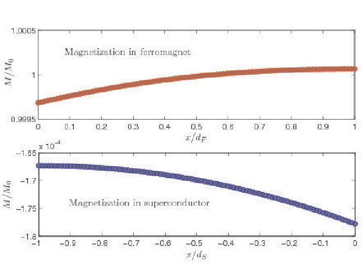
Let us first consider the temperature-dependence of the proximity-induced magnetization in the superconducting region in Fig. 13. To clarify the role of the spin-DIPS on each side of the interface, we plot for several values of in Fig. 13 (a) while keeping fixed. Conversely, we plot for several in Fig. 13 (b) with . In both cases, we plot the proximity-induced magnetization at . One obvious difference between these two scenarios is that the spin-DIPS on the superconducting side, , influence the proximity-induced magnetization much stronger than . The same thing is true with regard to the influence of spin-DIPS on the superconducting order parameter: influences the spatial profile of much more than what does. From Fig. 13, it is clearly seen how the proximity-induced magnetization may switch sign upon increasing the magnitude of the spin-DIPS . We have checked numerically that this effect also takes upon increasing when keeping . Thus, increasing either or can lead to a sign change of the proximity-induced magnetization in the superconducting region. It is then clear that the conclusion of Ref. [67] that only spin screening is possible in diffusive SF bilayers does not hold in general, since the presence of spin-DIPS alters the screening effect. In what follows, we focus on the role of since its impact on is much greater than that of . In Fig. 14, we consider the case to show that the sign change of the magnetization persists when going away from the limit . The spatial profile of the total magnetization in the F and S regions are shown for the case with in Fig. 15 and in Fig. 16. It is seen that the magnetization decreases in a monotonic fashion toward the superconducting region, and reaches its bulk value deep inside the ferromagnetic region. In the superconductor, magnetization is induced near the interface and decays with the distance from the interface.

III.3 Discussion
We propose the following explanation for the anti-screening effect observed upon increasing . The effect of the spin-DIPS in the case of a thin superconducting layer in Ref. [69] was shown to be equivalent to an internal magnetic exchange splitting in the superconducting region. Therefore, the magnitude of the magnetization in the superconductor should essentially grow with an increasing value of . If this is the case, the proximity-induced magnetization should also be sensitive to the sign of , as the opposite spin species would be energetically favored when comparing the case with . To test this hypothesis, we plot in Fig. 17 the proximity-induced magnetization at as a function of the spin-DIPS on the superconducting side, (keeping ). The results confirm our hypothesis – it is seen that is an antisymmetric function of . The influence of can also be seen directly in the LDOS in the superconducting region. For , we obtain a double-peak structure in the LDOS at in agreement with Refs. [69, 49], while the superconducting order parameter depletes very little close to the interface for the chosen parameter values. In general, the depletion of the superconducting order parameter is found to be small as long as and or smaller.
In Ref. [62], the inverse proximity effect of an SF bilayer was studied without taking into account the presence of spin-DIPS, with the result that the proximity-induced magnetization in the superconducting region would have the opposite sign of the proximity ferromagnet, i.e. a screening effect. It was proposed in Ref. [62] that this behavior could be understood physically by considering the contribution to the magnetization from Cooper pairs which were close to the interface: the spin- electron would prefer to be in the ferromagnetic region due to the exchange energy, while the spin- electron remaining in the superconducting region then would give rise to a magnetization in the opposite direction of the proximity ferromagnet. However, it is clear from the present study that this simple picture must be modified when properly considering the spin-DIPS on the superconducting side of the junction, since they act as an effective exchange field inside the superconductor.
In this paper, we have evaluated the proximity-induced magnetization in the vicinity of the interface without taking into account the Meissner response of the superconductor. This should be permissable in a thin-film geometry as the one employed in Ref. [63], where the screening currents are suppressed. In particular, for a field in the plane of the superconducting film (see Fig. 12), the Meissner effect should be strongly suppressed [71] for .
IV Summary
In conclusion, we have in Part I of this work investigated the proximity effect in a superconductorinhomogeneous ferromagnet junctions. Proper boundary conditions which take into account the spin dependent phase-shifts experienced by the reflected and transmitted quasiparticles were employed. As an application of our model, we have studied the LDOS in the ferromagnet in the presence of domain walls and a conical magnetic structure. We find that the presence of a domain wall enhances the odd-frequency correlations induced in the ferromagnet, manifested through a zero-energy peak in the LDOS. For the conical ferromagnet, we show that the spin-dependent phase shifts originating with the interface have a strong qualitative effect on the LDOS, especially for thin layers. In particular, we find an abrupt crossover from a fully suppressed LDOS to a finite LDOS which appears at a critical thickness of the ferromagnetic layer, and the particular value of the critical thickness depends on the value of . In a similar way, we find that there is an abrupt change appearing at a critical value of for sufficiently thin layers. We speculate that the reason for this could be a symmetry-transition from even- to odd-frequency correlations for the proximity-amplitudes in the ferromagnetic region. The theory developed in the present paper takes into account both the phase-shifts acquired by scattered quasiparticles at the interface due to the presence of ferromagnetic correlations, and also an arbitrary inhomogeneity of the magnetic texture on the ferromagnetic side. Our results for the conical ferromagnetic structure should be relevant for the material Ho, which was used in Ref. [57] to indicate the presence of long-range superconducting correlations.
In Part II of this work, we have investiged numerically and self-consistently the inverse proximity effect in a superconductorferromagnet (SF) bilayer, manifested through an induced magnetization in the superconducting region. We find that the interface properties play a crucial role in this context, as the spin-dependent interfacial phase-shifts (spin-DIPS) may invert the sign of the proximity-induced magnetization. This finding modifies previous conclusions obtained in the literature, and suggests that the influence of the spin-DIPS should be properly accounted for in a theory for the inverse proximity effect in SF bilayers.
Acknowledgements.
J.L. acknowledges M. Eschrig and A. Cottet for very useful discussions. J.L. and A.S. were supported by the Research Council of Norway, Grants No. 158518/432 and No. 158547/431 (NANOMAT), and Grant No. 167498/V30 (STORFORSK). T.Y. acknowledges support by JSPS.Appendix A Spin-active boundary conditions
To facilitate and encourage use of the spin-active boundary conditions required for an SF interface, we here write down their explicit form in the diffusive limit for the case of a magnetization in the -direction, following Ref. [48, 69]. Consider a junction consisting of two regions 1 and 2, as shown in Fig. 18. The regions have widths and bulk electrical resistances . The matrices used below are matrices in particle-holespin space, using a basis
Introducing , where is the third Pauli matrix in spin-space, we may write the boundary conditions as follows:
| (42) |

Here, is the conductance of the junction while are the phase-shifts on side of the interface. The parameters may be calculated by relating them to microscopic transmission and reflection probabilities within e.g. a Blonder-Tinkham-Klapwijk (BTK) [72] framework. Explicitly spin-active barriers were considered in ballistic SF bilayers using the BTK-approach for both -wave [73] and -wave [74] superconductors. In the absence of spin-DIPS , Eq. (42) reduce to the Kupriyanov-Lukichev non-magnetic boundary conditions [75]. Let us make a final remark concerning the treatment of interfaces in the quasiclassical theory of superconductivity. We previously stated that the application of the present theory requires that the characteristic energies of various self-energies and perturbations in the system are much smaller than the Fermi energy . At first glance, this might seem to be irreconcilable with the presence of interfaces, which represent strong perturbations varying on atomic length scales. However, this problem may be overcome by including the interfaces as boundary conditions for the Green’s functions rather than directly as self-energies in the Usadel equation.
References
- [1] F. S. Bergeret, A. F. Volkov, and K. B. Efetov, Rev. Mod. Phys. 77, 1321 (2005).
- [2] A. I. Buzdin, Rev. Mod. Phys. 77, 935-976 (2005).
- [3] F. S. Bergeret, A. F. Volkov, and K. B. Efetov, Phys. Rev. Lett. 86, 4096 (2001).
- [4] V. V. Ryazanov, V. A. Oboznov, A. Yu. Rusanov, A. V. Veretennikov, A. A. Golubov, and J. Aarts, Phys. Rev. Lett. 86, 2427 (2001).
- [5] A. F. Volkov, F. S. Bergeret, and K. B. Efetov, Phys. Rev. Lett. 90, 117006 (2003).
- [6] F. S. Bergeret, A. F. Volkov, and K. B. Efetov, Phys. Rev. B 68, 064513 (2003).
- [7] M. Eschrig, J. Kopu, J. C. Cuevas, and G. Schön, Phys. Rev. Lett. 90, 137003 (2003).
- [8] V. Braude and Yu. V. Nazarov, Phys. Rev. Lett. 98, 077003 (2007).
- [9] Y. Asano, Y. Tanaka, and A. A. Golubov, Phys. Rev. Lett. 98, 107002 (2007); Y. Asano, Y. Sawa, Y. Tanaka, and A. A. Golubov, Phys. Rev. B 76, 224525 (2007).
- [10] R. S. Keizer, S. T. B. Goennenwein, T. M. Klapwijk, G. Miao, G. Xiao, and A. Gupta, Nature (London) 439, 825 (2006).
- [11] Ya. V. Fominov, A. F. Volkov, and K. B. Efetov, Phys. Rev. B 75, 104509 (2007).
- [12] T. Yokoyama, Y. Tanaka, and A. A. Golubov, Phys. Rev. B 75, 134510 (2007).
- [13] Y. Asano, Y. Tanaka, A. A. Golubov, and S. Kashiwaya, Phys. Rev. Lett. 99, 067005 (2007).
- [14] K. Halterman, P. H. Barsic, and O. T. Valls, Phys. Rev. Lett. 99, 127002 (2007).
- [15] Y. Tanaka and A. A. Golubov, Phys. Rev. Lett. 98, 037003 (2007).
- [16] M. Eschrig, T. Lofwander, T. Champel, J. C. Cuevas, J. Kopu, G. Schön, J. Low Temp. Phys. 147, 457 (2007).
- [17] J. Linder, T. Yokoyama, and A. Sudbø, Phys. Rev. B 77, 174507 (2008); J. Linder, T. Yokoyama, Y. Tanaka, Y. Asano, and A. Sudbø, Phys. Rev. B 77, 174505 (2008).
- [18] M. Eschrig and T. Löfwander, Nature Phys. 4, 138 (2008).
- [19] K. Halterman, O. T. Valls, and P. H. Barsic, Phys. Rev. B 77, 174511 (2008).
- [20] J. Linder, T. Yokoyama, and A. Sudbø, Phys. Rev. B 77, 174514 (2008).
- [21] K. Yada, S. Onari, Y. Tanaka, and K. Miyake, arXiv:0806.4241.
- [22] L. N. Bulaevskii, V. V. Kuzii, and A. A. Sobyanin, Pis’ma Zh. Eksp. Teor. Fiz. 25, 314 (1977) [JETP Lett. 25, 290 (1977)].
- [23] A. I. Buzdin, L. N. Bulaevskii and S. V. Panyukov, Pis’ma Zh. Eksp. Teor. Fiz. 35, 147 (1982).
- [24] E. Koshina and V. Krivoruchko, Phys. Rev. B 63, 224515 (2001).
- [25] T. Kontos, M. Aprili, J. Lesueur, F. Genêt, B. Stephanidis, and R. Boursier, Phys. Rev. Lett. 89, 137007 (2002).
- [26] A. Buzdin and A. E. Koshelev, Phys. Rev. B 67, 220504 (2003).
- [27] M. Houzet, V. Vinokur, and F. Pistolesi, Phys. Rev. B 72, 220506 (2005).
- [28] A. Cottet and W. Belzig, Phys. Rev. B 72, 180503 (2005).
- [29] J. W. Robinson, S. Piano, G. Burnell, C. Bell, and M. G. Blamire, Phys. Rev. Lett. 97, 177003 (2006).
- [30] G. Mohammadkhani and M. Zareyan, Phys. Rev. B 73, 134503 (2006).
- [31] T. Yokoyama, Y. Tanaka, and A. A. Golubov, Phys. Rev. B 75, 094514 (2007).
- [32] M. Houzet and A. I. Buzdin, Phys. Rev. B 76, 060504 (2007).
- [33] B. Crouzy, S. Tollis, and D. A. Ivanov, Phys. Rev. B 75, 054503 (2007); Phys. Rev. B 76, 134502 (2007).
- [34] J. Linder, T. Yokoyama, D. Huertas-Hernando, and Asle Sudbø, Phys. Rev. Lett. 100, 187004 (2008).
- [35] T. Champel, M. Eschrig, Phys. Rev. B 71, 220506(R) (2005); T. Champel, M. Eschrig, Phys. Rev. B 72, 054523 (2005); T. Champel, T. Löfwander, and M. Eschrig, Phys. Rev. Lett. 100, 077003 (2008).
- [36] P. M. Brydon, B. Kastening, D. K. Morr, and D. Manske, Phys. Rev. B 77, 104504 (2008).
- [37] I. B. Sperstad, J. Linder, and A. Sudbø, Phys. Rev. B 78, 104509 (2008).
- [38] A. F. Volkov and K. B. Efetov, Phys. Rev. B 78, 024519 (2008).
- [39] V. L. Berezinskii, JETP Lett. 20, 287 (1974).
- [40] A. Balatsky and E. Abrahams, Phys. Rev. B 45, 13125 (1992).
- [41] P. Coleman, E. Miranda, and A. Tsvelik, Phys. Rev. Lett. 70, 2960 (1993).
- [42] E. Abrahams, A. Balatsky, D. J. Scalapino, and J. R. Schrieffer, Phys. Rev. B 52, 1271 (1995).
- [43] D. Solenov, I. Martin, D. Mozyrsky, arXiv:0812.1055.
- [44] J. Y. Gu, J. A. Caballero, R. D. Slater, R. Loloee, and W. P. Pratt, Jr., Phys. Rev. B 66, 140507 (2002).
- [45] M. A. Sillanpaa, T. T. Heikkila, R. K. Lindell, and P. J. Hakonen, Europhys. Lett. 56, 590 (2001).
- [46] F. S. Bergeret, A. Levy Yeyati, A. Martin-Rodero, Phys. Rev. B 72, 064524 (2005).
- [47] J. P. Morten, A. Brataas, G. E. W. Bauer, W. Belzig, Y. Tserkovnyak, arXiv:0712.2814v1.
- [48] D. Huertas-Hernando, Yu. V. Nazarov, and W. Belzig, Phys. Rev. Lett. 88, 047003 (2002); D. Huertas-Hernando and Yu. V. Nazarov, Eur. Phys. J. B 44, 373 (2005).
- [49] A. Cottet and J. Linder, arXiv:0810.0904.
- [50] P. SanGiorgio, S. Reymond, M. R. Beasley, J. H. Kwon, and K. Char, Phys. Rev. Lett. 100, 237002 (2008).
- [51] See e.g. J. W. Serene and D. Rainer, Phys. Rep. 101, 221 (1983).
- [52] K. Usadel, Phys. Rev. Lett. 25, 507 (1970).
- [53] D. A. Ivanov and Ya. V. Fominov, Phys. Rev. B 73, 214524 (2006).
- [54] N. Schopohl and K. Maki, Phys. Rev. B 52, 490 (1995); N. Schopohl, cond-mat/9804064.
- [55] A. Konstandin, J. Kopu, and M. Eschrig, Phys. Rev. B 72, 140501 (2005).
- [56] A. Brataas, Yu. V. Nazarov, and G. E. W. Bauer, Phys. Rev. Lett. 84, 2481 (2000); Eur. Phys. J. B 22, 99 (2001); A. Brataas, G. E. W. Bauer, and P. J. Kelly, Phys. Rep. 427, 157 (2006).
- [57] I. Sosnin, H. Cho, V. T. Petrashov, and A. F. Volkov, Phys. Rev. Lett. 96, 157002 (2006).
- [58] T. Yokoyama, Y. Tanaka, and A. A. Golubov, Phys. Rev. B 72, 052512 (2005); Phys. Rev. B 73, 094501 (2006).
- [59] T. Kontos, M. Aprili, J. Lesueur, and X. Grison, Phys. Rev. Lett. 86, 304 (2001).
- [60] J. Linder, T. Yokoyama, A. Sudbø, and M. Eschrig, unpublished.
- [61] C. Bruder, Phys. Rev. B 41, 4017 (1990).
- [62] F. S. Bergeret, A. F. Volkov, and K. B. Efetov, Phys. Rev. B 69, 174504 (2004).
- [63] J. Xia, V. Shelukhin, M. Karpovski, A. Kapitulnik, and A. Palevski, arXiv:0810.2605.
- [64] Th. Muehge, N. N. Garif’yanov, Yu. V. Goryunov, K. Theis-Bröhl, K. Westerholt, I. A. Garifullin, and H. Zabel, Physica C 296, 325 (1998).
- [65] I. A. Garifullin, D. A. Tikhonov, N. N. Garif’yanov, M. Z. Fattakhov, K. Theis- Bröhl, K. Westerholt, and H. Zabel, Appl. Magn. Reson. 22, 439 (2002).
- [66] R. I. Salikhov, I. A. Garifullin, N. N. Garif’yanov, L. R. Tagirov, K. Theis-Bröhl, K. Westerholt, H. Zabel, arXiv:0806.4104.
- [67] M. Yu. Kharitonov, A. F. Volkov, K. B. Efetov, Phys. Rev. B 73, 054511 (2006).
- [68] K. Halterman and O. T. Valls, Phys. Rev. B 69, 014517 (2004).
- [69] A. Cottet, Phys. Rev. B 76, 224505 (2007).
- [70] J. Linder and A. Sudbø, Phys. Rev. B 76, 214508 (2007).
- [71] R. Meservey and P. M. Tedrow, Phys. Rep. 238, 173 (1994).
- [72] G. E. Blonder, M. Tinkham, and T. M. Klapwijk, Phys. Rev. B 25, 4515 (1982).
- [73] J. Linder and A. Sudbø, Phys. Rev. B 75, 134509 (2007).
- [74] S. Kashiwaya, Y. Tanaka, N. Yoshida, and M. R. Beasley, Phys. Rev. B 60, 3572 (1999).
- [75] M. Yu. Kupriyanov and V. F. Lukichev, Zh. Exp. Teor. Fiz. 94, 139 (1988) [Sov. Phys. JETP 67, 1163 (1988)].