ENTROPY, TRIANGULATION, AND POINT LOCATION
IN PLANAR SUBDIVISIONS

Sébastien Collette
Université Libre de Bruxelles ^†^†thanks: Chargé de Recherches du F.R.S.-FNRS. Vida Dujmović
Carleton University ^†^†thanks: Research partially supported by NSERC and the Ontario Ministry of Research and Innovation. John Iacono
Polytechnic Institute of NYU ^†^†thanks: Research partially supported by NSF grants OISE-0334653 and CCF-0430849 and by an Alfred P. Sloan research fellowship. Stefan Langerman
Université Libre de Bruxelles ^†^†thanks: Maître de recherches du F.R.S.-FNRS. Pat Morin
Carleton University ^†^†thanks: This research began while the author was a visiting researcher at the Université Libre de Bruxelles and was completed while the author was a visiting researcher at National ICT Australia and the University of Sydney. Research partially supported by NSERC, FNRS, the Ontario Ministry of Research and Innovation, Canada Foundation for Innovation, The University of Sydney, and National ICT Australia.

Abstract

A data structure is presented for point location in connected planar subdivisions when the distribution of queries is known in advance. The data structure has an expected query time that is within a constant factor of optimal. More specifically, an algorithm is presented that preprocesses a connected planar subdivision $G$ of size $n$ and a query distribution $D$ to produce a point location data structure for $G$ . The expected number of point-line comparisons performed by this data structure, when the queries are distributed according to $D$ , is $\tilde{H}+O(\tilde{H}^{2/3}+1)$ where $\tilde{H}=\tilde{H}(G,D)$ is a lower bound on the expected number of point-line comparisons performed by any linear decision tree for point location in $G$ under the query distribution $D$ . The preprocessing algorithm runs in $O(n\log n)$ time and produces a data structure of size $O(n)$ . These results are obtained by creating a Steiner triangulation of $G$ that has near-minimum entropy.

1 Introduction

The planar point location problem is the classic search problem in computational geometry. Given a planar subdivision $G$ ,¹¹ 1 A planar subdivision is a partitioning of the plane into points (called vertices), open line segments (call edges), and maximal connected 2-dimensional regions (called faces). the planar point location problem asks us to construct a data structure so that, for any query point $q$ , we can quickly determine which face of $G$ contains $q$ .²² 2 In the degenerate case where $q$ is a vertex or contained in an edge of $G$ any face incident on that vertex/edge may be returned as an answer.

The history of the planar point location problem parallels, in many ways, the history of binary search trees. After a few initial attempts [11, 18, 21], asymptotically optimal (and quite different) linear-space $O(\log n)$ query time solutions to the planar point location problem were obtained by Kirkpatrick [17], Sarnak and Tarjan [24], and Edelsbrunner et al. [12] in the mid 1980s. These results were based on hierarchical simplification, data structural persistence, and fractional cascading, respectively. All three of these techniques have subsequently found many other applications. An elegant randomized solution, combining aspects of all three previous solutions, was later given by Mulmuley [20], and uses randomized incremental construction, a technique that has since become pervasive in computational geometry [10, Section 9.5]. Preparata [22] gives a comprehensive survey of the results of this era.

In the 1990s, several authors became interested in determining the exact constants achievable in the query time. Goodrich et al. [13] gave a linear-size data structure that, for any query, requires at most $2\log n+o(\log n)$ point-line comparisons and conjectured that this query time was optimal for linear-space data structures.³³ 3 Here and throughout, logarithms are implicitly base 2 unless otherwise specified. The following year, Adamy and Seidel [1] gave a linear-space data structure that answers queries using $\log n+2\sqrt{\log n}+O(\log\log n)$ point-line comparisons and showed that this result is optimal up to the third term.

Still not done with the problem, several authors considered the point location problem under various assumptions about the query distribution. All these solutions compare the expected query time to the entropy bound; in a planar subdivision $G$ with $m$ faces $F_{1},\ldots,F_{m}$ , if $\Pr(F_{i})$ is the probability that $q$ is contained in $F_{i}$ , then no algorithm that makes only binary decisions can answer queries using an expected number of decisions that is fewer than

H=H(G,D)=\sum_{i=1}^{m}\Pr(F_{i})\log(1/\Pr(F_{i}))\kern 5.0pt.

(1)

In the previous results on planar point location, none of the query times are affected significantly by the structure of $G$ ; they hold for arbitrary planar subdivisions. However, when studying point location under a distribution assumption the problem becomes more complicated and the results become more specific. A connected subdivision is a planar subdivision whose underlying (vertex and edge) graph is connected. A convex subdivision is a planar subdivision whose faces are all convex polygons, except the outer face, which is the complement of a convex polygon. A triangulation is a convex subdivision in which each face has at most 3 edges on its boundary.

Note that, if every face of $G$ has a constant number of sides, then $G$ can be augmented, by the addition of extra edges, so that it is a triangulation without increasing (1) by more than a constant. Similarly, in a convex subdivision $G$ where the query distribution $D$ is uniform within each face of $G$ , the faces of the subdivision can be triangulated without increasing the entropy by more than a constant [3]. Thus, in the following we will simply refer to results about triangulations where it is understood that these also imply the same result for planar subdivisions with faces of constant size or convex subdivisions when the query distribution is uniform within each face.

Arya et al. [2] gave two results for the case where the query point $p$ is chosen from a known distribution where the $x$ and $y$ coordinates of $p$ are chosen independently and $G$ is a convex subdivision. They gave an $O(n)$ space data structure for which the expected number of point-line comparisons is at most $4H+O(1)$ and an $O(n^{2})$ space data structure for which the expected number of point-line comparisons is at most $2H+O(1)$ . The assumption about the independence of the $x$ and $y$ coordinates of $p$ is crucial to the these results.

For arbitrary distributions that are known in advance, several results exist. Iacono [15, 16] showed that, for triangulations, a simple variant of Kirkpatrick’s original point location structure gives a linear space, $O(H+1)$ expected query time data structure. Simultaneously, and independently, Arya et al. [5] showed that a variant of Mulmuley’s randomized data structure also achieves $O(H+1)$ expected query time. A sequence of papers by Arya et al. [3, 4, 6] has recently culminated in an $O(n)$ space data structure for point location in triangulations with query time $H+O(H^{1/2}+1)$ [6].

In the current paper, we show that, for any connected planar subdivision, there exists a data structure of size $O(n)$ that can answer point location queries using $\tilde{H}+O(\tilde{H}^{2/3}+1)$ point/line comparisons. Here, $\tilde{H}=\tilde{H}(G,D)$ is a lower bound on the expected cost of any linear decision tree that solves this problem. Note that $\tilde{H}$ is often greater than the quantity $H$ defined above and this is necessarily so. To see this, consider that the problem of testing whether a query point is contained in a simple polygon $P$ with $n$ vertices is a special case of planar point location in a connected planar subdivision. However, in this special case the subdivision only has 2 faces, so $H\leq 1$ . It seems unlikely that, for any simple polygon $P$ and any probability measure $D$ over $\mathbb{R}^{2}$ , it is always possible to test in $O(1)$ expected time if a point $p$ drawn from $D$ is contained in $P$ . Indeed, it is not hard to design a convex polygon $P$ and distribution $D$ so that the expected cost of any algebraic decision tree for point location in $P$ , under query distribution $D$ , is $\Omega(\log n)$ .

Note that all known algorithms for planar point location that do not place special restrictions on the input subdivision can be described in the linear decision tree model of computation.⁴⁴ 4 Although significant breakthroughs have recently been made in this area [8, 23], we deliberately do not survey algorithms that require the vertices of the subdivision to be on integer coordinates. The data structures presented in the current paper are the most general results known about planar point location and imply, to within a lower order term, all of the results discussed in the introduction.

We achieve our results by showing how to compute a Steiner triangulation $\Delta=\Delta(G,D)$ of $G$ that has nearly minimum entropy over all possible triangulations of $G$ and then proving that the entropy of a minimum-entropy Steiner triangulation of $G$ is a lower bound on the cost of any linear decision tree for point location in $G$ . By then applying the recent result of Arya et al. to the Steiner triangulation $\Delta$ we obtain upper and lower bounds that match to within a lower-order term.

A preliminary version of this paper, which dealt only with convex subdivisions, has appeared in the Proceedings of the 19th ACM-SIAM Symposium on Discrete Algorithms (SODA 2008) [9].

The remainder of this paper is organized as follows: Section 2 presents definitions and notations used throughout the paper. Section 3 shows how to compute a near-minimum-entropy triangulation of a simple polygon. Finally, Section 4 applies these tools to obtain our point location structure for connected planar subdivisions.

2 Preliminaries

In this section we give definitions, notation, and background required in subsequent sections.

Interiors and Boundaries.

For a set $P\subseteq\mathbb{R}^{2}$ , we denote the boundary of $P$ by $\partial P$ and the interior of $P$ by $\mathrm{int}(P)$ . The closure of $P$ is denoted by $\mathrm{clo}(P)=P\cup{\partial P}$ .

Triangles and Convex Polygons.

For the purposes of this paper, a triangle is the common intersection of at most 3 closed halfplanes. This includes triangles with infinite area and triangles having 0, 1, 2, or 3, vertices. Similarly, a convex $k$ -gon is the common intersection of at most $k$ closed halfplanes.

For a closed region $X\subseteq\mathbb{R}^{2}$ , a triangulation of $X$ is a set of triangles whose interiors are pairwise disjoint and whose union is $X$ . We use the convention that, unless $X$ is explicitly mentioned, the triangulation in question is a triangulation of $\mathbb{R}^{2}$ . This definition of a triangulation is often referred to as a Steiner triangulation since it allows vertices of the triangles to be anywhere in $X$ , and not at some finite predefined set of locations.

Simple Polygons, Pseudotriangles, and Geodesic Triangles.

A (near-simple) polygon $P$ is a closed subset of $\mathbb{R}^{2}$ whose boundary is piecewise linear and such that $\mathrm{int}(P)$ is homeomorphic to an open disk. Note that this definition of a polygon implies that every bounded face of a connected planar subdivision is a polygon. Also, triangles, as defined above, are polygons. Note that near-simple polygons are slightly more general than simple polygons, for which $\partial P$ is a simple closed curve. However, our definition is sufficiently close that algorithms designed for simple polygons continue to work with near-simple polygons.

A reflex chain in a polygon $P$ is a consecutive sequence of vertices $p_{i},\ldots,p_{j}$ of $P$ , where the internal angle at $p_{k}$ is at least $\pi$ , for all $k\in\{i+1,\ldots,j-1\}$ . A pseudotriangle is a polygon whose boundary consists of 3 reflex chains. An $i$ -convex pseudotriangle ( $i\in\{0,1,2,3\}$ ) is a pseudotriangle in which $i$ of the reflex chains consist of single line segments.

A shortest path between points $a,b\in P$ , denoted $\overline{ab}_{P}$ is a curve of minimum length that is contained in $P$ and that has $a$ and $b$ as endpoints. For 3 points, $a,b,c\in P$ , a geodesic triangle in $P$ , denoted $\triangle_{P}abc$ is the union of all shortest paths of the form $\overline{xc}_{P}$ , where $x\in\overline{ab}_{P}$ . Geodesic triangles are closely related to pseudotriangles. In particular, every geodesic triangle $t$ consists of a pseudotriangle ${\hat{t}}$ and three paths joining the three convex vertices of ${\hat{t}}$ to $a$ , $b$ , and $c$ .

Classification Problems and Classification Trees.

A classification problem over a domain $\mathcal{D}$ is a function $\mathcal{P}:\mathcal{D}\mapsto\{0,\ldots,k-1\}$ . A $d$ -ary classification tree is a full $d$ -ary tree⁵⁵ 5 A full $d$ -ary tree is a rooted ordered tree in which each non-leaf node has exactly $d$ children. in which each internal node $v$ is labelled with a function $P_{v}:\mathcal{D}\mapsto\{0,.\ldots,d-1\}$ and for which each leaf $\ell$ is labelled with a value $d(\ell)\in\{0,\ldots,k-1\}$ . The search path of an input $p$ in a classification tree $T$ starts at the root of $T$ and, at each internal node $v$ , evaluates $i=P_{v}(p)$ and proceeds to the $i$ th child of $v$ . We denote by $T(p)$ the label of the final (leaf) node in the search path for $p$ . We say that the classification tree $T$ solves the classification problem $\mathcal{P}$ over the domain $\mathcal{D}$ if, for every $p\in\mathcal{D}$ , $\mathcal{P}(p)=T(p)$ .

In this paper, we are especially concerned with linear decision trees. These are binary classification trees for a problem $\mathcal{P}$ over the domain $\mathbb{R}^{2}$ . Each internal node $v$ of a linear decision tree contains a linear inequality $P_{v}(x,y)=ax+by\geq c$ , and the node evaluates to 1 or 0 depending on whether the query point $(x,y)$ satisfies the inequality or not, respectively. Geometrically, each internal node of $T$ is labelled with a directed line and the decision to go to the left or right child depends on whether $p$ is to the left or right (or on) this line. An immediate consequence of this is that, for each leaf $\ell$ of $T$ , the closure of $r(\ell)$ is a convex polygon.

Probability.

Throughout this paper $D$ is a probability measure over $\mathbb{R}^{2}$ that represents the query distribution. The notation $\Pr(X)$ denotes the probability of event $X$ under the probability measure $D$ . The notation $\Pr(Y|X)$ denotes the conditional probability of $Y$ given $X$ , i.e., $\Pr(Y|X)=\Pr(Y\cap X)/\Pr(X)$ . For any set $S$ , we use the shorthand $\cup S$ to denote $\bigcup_{s\in S}s$ .

For a set $S$ of subsets of $\mathbb{R}^{2}$ , we define the induced entropy of $S$ , denoted by $H(S)$ as $H(S)=\sum_{s\in S}\Pr(s|{\cup S})\log(1/\Pr(s|{\cup S}))$ . For two sets $S_{1},S_{2}\subseteq\mathbb{R}^{2}$ with $\cup S_{1}=\cup S_{2}$ , the joint entropy of $S_{1}$ and $S_{2}$ , is $H(S_{1},S_{2})=\sum_{s_{1}\in S_{i}}\sum_{s_{2}\in S_{2}}\Pr(s_{1}\cap s_{2})\log(1/\Pr(s_{1}\cap s_{2}))$ . It is well-known that $H(S_{1},S_{2})\leq H(S_{1})+H(S_{2})$ (see, for example, Gray [14, Lemma 2.3.2]).

We will sometimes abuse terminology slightly by referring to a triangulation $\Delta$ of $X$ as a partition of $X$ into triangles, although strictly speaking this is not true since the triangles in $\Delta$ are closed sets that overlap at their boundaries. We will then continue the abuse by computing the induced entropy of $\Delta$ . This introduces a technical difficulty in that $\sum_{t\in\Delta}\Pr(t)\geq 1$ and inequality is possible if there exists sets $Y\subset\mathbb{R}^{2}$ such that the area of $Y$ is 0 and $\Pr(Y)>0$ . To avoid this technical difficulty, we will assume that $D$ is nice in the sense that, if the area of $Y$ is 0 then $\Pr(Y)=0$ . This implies that, for every $t$ in $\Delta$ $\Pr(t)=\Pr(\mathrm{int}(t))$ . This assumption will avoid lengthy technical but uninteresting cases in our analysis. In practice, this problem can be avoided by using a symbolic perturbation of the query point.

The probability measures used in this paper are usually defined over $\mathbb{R}^{2}$ . We make no assumptions about how these measures are represented, but we assume that an algorithm can, in constant time, perform each of the following two operations:

1.

given a triangle $t$ , compute $\Pr(t)$ , and
2.

given a triangle $t$ and a point $x$ at the intersection of two of $t$ ’s supporting lines, compute a line $\ell$ that contains $x$ and that partitions $t$ into two open triangles $t_{0}$ and $t_{1}$ such that $\Pr(t_{0})\leq\Pr(t_{1})\leq\Pr(t)/2$ .

Requirement 2 is used only for convenience in describing our data structure. It is not strictly necessary, but its use greatly simplifies the exposition of our results. To eliminate requirement 2, one can use the same method described by Collette et al. [9, Section 5].

For a classification tree $T$ that solves a problem $P:\mathcal{D}\mapsto\{0,\ldots,k-1\}$ and a probability measure $D$ over $\mathcal{D}$ , the expected search time of $T$ is the expected length of the search path for $p$ when $p$ is drawn at random from $\mathcal{D}$ according to $D$ . Note that, for each leaf $\ell$ of $T$ there is a maximal subset $r(\ell)\subseteq\mathcal{D}$ such that the search path for any $p\in r(\ell)$ ends at $\ell$ . Thus, the expected search time of $T$ (under distribution $D$ ) can be written as

\mu_{D}(T)=\sum_{\ell\in L(T)}\Pr(r(\ell))\times 0pt(\ell)\kern 5.0pt,

where $L(T)$ denotes the leaves of $T$ and $0pt(\ell)$ denotes the length of the path from the root of $T$ to $\ell$ . For any tree $T$ we use $V(T)$ to denote the vertices of $T$ .

The following theorem, which is a restatement of (half of) Shannon’s Fundamental Theorem for a Noiseless Channel [25, Theorem 9], is what all previous results on distribution-sensitive planar point location use to establish their optimality:

Theorem 1 (Fundamental Theorem for a Noiseless Channel).

Let $\mathcal{P}:\mathcal{D}\mapsto\{0,\ldots,k-1\}$ be a classification problem and let $p\in\mathcal{D}$ be selected from a distribution $D$ such that $\Pr\{\mathcal{P}(p)=i\}=p_{i}$ , for $0\leq i<k$ . Then, any $d$ -ary classification tree $T$ that solves $\mathcal{P}$ has

\mu_{D}(T)\geq\sum_{i=0}^{k-1}p_{i}\log_{d}(1/p_{i})\kern 5.0pt.

(2)

Theorem 1 is typically applied to the point location problem by treating point location as the problem of classifying the query point $p$ based on which face of $G$ contains it. In this way, we obtain the lower bound in (1).

3 Minimum Entropy Triangulations

Let $P$ be a simple polygon with $n$ vertices, denoted $p_{0},\ldots,p_{n-1}$ as they occur, in counterclockwise order, on the boundary of $P$ . We will show how to find a triangulation of $P$ that has near-minimum entropy. That is, we will find a triangulation $\Delta=\Delta(P,D)$ such that $H(\Delta)$ is near-minimum over all triangulations of $P$ . In order to shorten the formulas in this section, we will implicitly condition the distribution $D$ on $P$ . More precisely, throughout this section the notation $\Pr(X)$ should be treated as shorthand for $\Pr(X|P)$ .

3.1 The Triangulation $\Delta=\Delta(P,D)$

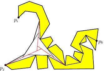
Our triangulation algorithm is recursive and takes as input a polygon $P$ and a reflex chain $p_{i},\ldots,p_{j}$ on the boundary of $P$ . If $P$ is a triangle, then there is nothing to do, so the algorithm outputs $P$ and terminates. Otherwise, the algorithm first selects a point $p_{k}$ on the boundary of $P$ and adds all the edges of the geodesic triangle $t=\triangle p_{i}p_{j}p_{k}$ to the triangulation $\Delta$ . Observe that removing $t$ from $P$ disconnects $P$ into components $P_{1},\ldots,P_{m}$ where $\mathrm{clo}(P_{i})$ is a polygon that shares a reflex chain $C_{i}$ with the pseudotriangle $t$ (see Figure 1). The point $p_{k}$ is selected in such a way that, for all $i\in\{1,\ldots,m\}$ , $\Pr(P_{i})\leq(1/2)\Pr(P)$ .⁶⁶ 6 The existence of such a point $p_{k}$ is readily established by a standard continuity argument; see Bose et al. [7] for an example. Each of the sub-polygons $P_{1},\ldots,P_{m}$ can then be triangulated recursively by applying the algorithm to $P_{i}$ and the reflex chain $C_{i}$ .

Refer to caption — Figure 1: The geodesic triangle $t=\triangle p_{i}p_{j}p_{k}$ partitions $P$ into several pieces $P_{1},\ldots,P_{m}$ .

To complete the triangulation $\Delta$ all that remains is to partition ${\hat{t}}=\mathrm{clo}(t\setminus\partial t)$ into triangles. To do this, we first partition ${\hat{t}}$ into at most one triangle $t^{\prime}$ and three 2-convex pseudotriangles $t_{0},t_{1},t_{2}$ as shown in Figure 2.a. Let $Q_{i}$ be the connected component of $(\mathrm{int}(P)\setminus{\hat{t}})\cup t_{i}$ that contains $t_{i}$ . To complete the triangulation we will partition $t_{i}$ into triangles, for each $i\in\{0,1,2\}$ , using a recursive algorithm. This algorithm selects an edge $e_{i}$ of the reflex chain in $t_{i}$ and extends $e_{i}$ in both directions until it reaches the boundary of $t_{i}$ (see Figure 2.b). The resulting line segment partitions $t_{i}$ into a triangle $t_{i}^{\prime}$ , and two 2-convex pseudotriangles $t_{i,0}$ and $t_{i,1}$ that are triangulated recursively. At the same time, $Q_{i}$ is partitioned into up to 4 pieces (see Figure 2.c):

1.

the triangle $t_{i}^{\prime}$ , and
2.

a subpolygon $P_{j}$ incident to $e_{i}$ ,
3.

The two connected components $Q_{i,0}$ and $Q_{i,1}$ of $Q_{i}\setminus t_{i}^{\prime}$ that contain $t_{i,0}$ and $t_{i,1}$ , respectively.

The edge $e_{i}$ is selected so that $\Pr(Q_{i,b})\leq(1/2)\Pr(Q_{i})$ for each $b\in\{0,1\}$ .⁷⁷ 7 The existence of such an edge $e_{i}$ is assured by yet another continuity argument. This completes the description of the triangulation $\Delta$ . A partially completed triangulation is show in Figure 3.

3.2 The $\Delta$ -Tree $T=T(P,D)$

In order to study the entropy of the triangulation $\Delta$ defined above, we will impose a tree structure on the pieces of $P$ induced by the triangles in $\Delta$ . The $\Delta$ -tree $T=T(P,D)$ for $P$ is a tree whose nodes are subpolygons of $P$ and which has the property that, for any node $y$ that is the child of a node $x$ , $y\subseteq x$ .

The tree $T$ has three different kinds of nodes, called P-nodes, T-nodes, and Q-nodes. The root $r$ of $T$ is the polygon $P$ and is a P-node. The root of $T$ has the following children (defined in terms of the construction algorithm in the previous section; see Figure 4):

1.

Each subpolygon $P_{i}$ whose boundary does not share a segment with ${\hat{t}}$ is a child of $r$ and is a P-node.
2.

The subpolygon $Q={\hat{t}}\cup Q_{0}\cup Q_{1}\cup Q_{2}$ is a child of $r$ and is called a T-node.

The subpolygon $Q$ has three children $Q_{0},Q_{1},Q_{2}$ that are called Q-nodes. The subtree rooted at $Q_{i}$ is a ternary tree corresponding to the recursive partitioning of $t_{i}$ and $Q_{i}$ done by the algorithm. The leaves of this subtree are P-nodes and the internal nodes of this subtree are Q-nodes. Each internal node has up to 3 children, up to 1 of which may be a P-node corresponding to a subpolygon $P_{j}$ and up to two of which may be Q-nodes.

Note that the above definition yields a tree whose leaves are P-nodes that correspond to the subpolygons $P_{1},\ldots,P_{m}$ obtained by removing $t$ from $P$ . The subtree rooted at each such leaf is obtained recursively from the recursive triangulation of $P_{i}$ .

Now that we have defined the tree $T$ , we study some of its properties. Our first lemma says that $T$ does a good job of splitting $P$ based on its probabilities.

Lemma 1.

Let $P$ be a polygon, let $D$ be a probability measure over $\mathbb{R}^{2}$ , and let $T=T(P,D)$ be the $\Delta$ -tree for $(P,D)$ . Let $x$ be a node of $T$ whose depth is $i$ . Then $\Pr(x)\leq(1/2^{{\left\lfloor i/4\right\rfloor}})\Pr(P)$ .

Proof.

Assume $i\geq 4$ , otherwise there is nothing to prove. Let $r^{\prime}$ be the fourth node on the path from the root, $r$ , of $T$ to $x$ . Let $P_{r^{\prime}}$ be the path in $T$ from $r$ to $r^{\prime}$ . If $P_{r^{\prime}}$ has at least two P-nodes, then $\Pr(r^{\prime})\leq(1/2)\Pr(r)=(1/2)\Pr(P)$ . Otherwise, the second node in $P_{r^{\prime}}$ is a T-node followed by 2 Q-nodes. By construction, for any Q-node $y$ whose parent is a Q-node $z$ , $\Pr(y)\leq(1/2)\Pr(z)$ . Therefore, $\Pr(r^{\prime})\leq(1/2)\Pr(\mathrm{parent}(r^{\prime}))\leq(1/2)\Pr(r)=(1/2)\Pr(P)$ . If $x=r^{\prime}$ , then $i=4$ and the proof is complete. Otherwise, apply the same argument inductively on the path from $r^{\prime}$ to $x$ , to obtain

\Pr(x)\leq\Pr(r^{\prime})\cdot 1/2^{{\left\lfloor(i-4)/4\right\rfloor}}=\Pr(r^{\prime})\cdot 1/2^{{\left\lfloor i/4\right\rfloor}-1}\leq(1/2^{{\left\lfloor i/4\right\rfloor}})\Pr(r)=(1/2^{{\left\lfloor i/4\right\rfloor}})\Pr(P)\kern 5.0pt,

and this completes the proof. ∎

Our next lemma says that a single line segment does not intersect very many high probability triangles in $\Delta$ .

Lemma 2.

Let $P$ be a polygon, let $D$ be a probability measure over $\mathbb{R}^{2}$ , and let $T=T(P,D)$ be the $\Delta$ -tree for $(P,D)$ , let $s\subseteq P$ be a line segment, and let $S_{i}\subseteq V(T)$ be the set of all vertices $x\in V(T)$ that are distance at most $i$ from the root of $T$ and such that $\mathrm{int}(x)$ intersect $s$ . Then $|S_{i}|\leq 6i^{2}$

Proof.

There are 3 types of nodes in $T$ whose interiors intersect $s$ : Type 1 nodes contain one endpoint of $s$ in their interior, Type 2 nodes contain both endpoints of $s$ in their interior, and Type 0 nodes contain no endpoints of $s$ in their interior. Notice that each level of $T$ contains at most 1 Type 2 node or 2 Type 1 nodes, so the total number of Type 1 and Type 2 nodes at distance at most $i$ from the root is at most $2i+1$ . Thus, all that remains is to bound the number of Type 0 nodes whose distance from the root is at most $i$ .

Let $w$ be any P-node such that $\mathrm{int}(w)$ does not contain either endpoint of $s$ . Since $w$ is a P-node, there is a reflex chain $C_{w}$ on the boundary of $w$ that is a shortest path between two points on the boundary of $P$ , and every path in $P$ from $\mathrm{int}(w)$ to $s$ intersects $C_{w}$ . Stated another way, the interior of a P-node does not intersect $s$ unless it contains at least one endpoint of $s$ . Therefore, all Type 0 nodes are either T-nodes or Q-nodes.

For every Type 0 node $x$ , there is a path $P_{x}$ in $T$ from $x$ to a T-node that is adjacent to a Type 1 or Type 2 node. Furthermore, the path $P_{x}$ consists of $x$ followed by 0 or more Q-nodes, and terminates with a T-node. Looking more closely at the definition of Q-nodes, we see that two sibling Q-nodes $x$ and $y$ are not mutually visible, i.e., there is no line segment $s\subseteq P$ that intersects both $\mathrm{int}(x)$ and $\mathrm{int}(y)$ .

All of this implies that each of the at most $2i+1$ Type 1 or Type 2 nodes is adjacent to at most 1 Type 0 T-node, and this T-node is the endpoint of at most 3 paths of Type 0 Q-nodes. Each such path is of length at most $i$ . Therefore, the total number of nodes in $T$ that intersect $s$ is at most $2i\cdot 3i=6i^{2}$ . ∎

3.3 Minimum-Entropy Triangulation

Next, we show that the triangulation $\Delta$ defined above is nearly-minimum entropy over all possible triangulations of $P$ . We do this by developing a technique for lower-bounding the entropy of one triangulation in terms of the entropy of another triangulation. We then show how to apply this technique to lower bound the entropy of any triangulation $\Delta^{*}$ in terms of the entropy of $\Delta$ .

To obtain lower bounds on the entropy of a triangulation $\Delta^{*}$ , consider the following easily proven observation: If each triangle in $\Delta^{*}$ intersects at most $c$ triangles of some triangulation $\Delta$ then $H(\Delta^{*})\geq H(\Delta)-\log c$ .⁸⁸ 8 Proof: Consider the set $X=\{t^{*}\cap t:t^{*}\in\Delta^{*},t\in\Delta\}$ . Each triangle of $\Delta^{*}$ contributes at most $c$ pieces to $X$ , so we have $H(\Delta)\leq H(X)\leq H(\Delta^{*})+\log c$ . This observation allows us to use $\Delta$ to prove a lower bound on the entropy of a triangulation $\Delta^{*}$ . Unfortunately, the condition that each triangle of $\Delta^{*}$ intersect at most $c$ triangles of $\Delta$ is too restrictive for our purposes. Instead, we require following stronger result:

Lemma 3.

Let $D$ be a probability measure over $\mathbb{R}^{2}$ . Let $\Delta$ and $\Delta^{*}$ be triangulations, and let $\{\Delta_{1},\ldots,\Delta_{m}\}$ be a partition of the triangles in $\Delta$ . Suppose that, for all $i\in\{1,\ldots,m\}$ and for each triangle $t^{*}\in\Delta^{*}$ , $t^{*}$ intersects at most $c_{i}$ triangles in $\Delta_{i}$ . Then

\displaystyle H(\Delta)\leq H(\Delta^{*})+H(\{\cup\Delta_{1},\ldots,\cup\Delta_{m}\})+\sum_{i=1}^{m}\Pr(\cup\Delta_{i})\log c_{i}\kern 5.0pt.

Intuitively, Lemma 3 can be thought of as follows: If we tell an observer which of the $\Delta_{i}$ a point $p$ drawn according to $D$ occurs in then the amount of information we are giving the observer about the experiment is at most $H(\{\cup\Delta_{1},\ldots,\cup\Delta_{m}\})$ . However, after giving away this information, we are able to apply the simple observation in the previous paragraph, since each triangle in $\Delta^{*}$ intersects at most $c_{i}$ elements of each $\Delta_{i}$ . Thus, Lemma 3 is really just $m$ applications of the simple observation. The following proof formalizes this:

Proof.

$\displaystyle H(\Delta^{*})+H(\{\cup\Delta_{1},\ldots,\cup\Delta_{m}\})$	$\displaystyle\geq$	$\displaystyle H(\Delta^{*},\{\cup\Delta_{1},\ldots,\cup\Delta_{m}\})$
	$\displaystyle=$	$\displaystyle\sum_{i=1}^{m}\sum_{t^{}\in\Delta^{}}\Pr(t^{}\cap\Delta_{i})\log(1/\Pr(t^{}\cap\Delta_{i})$
	$\displaystyle\geq$	$\displaystyle\sum_{i=1}^{m}\sum_{t\in\Delta_{i}}\sum_{t^{}\in\Delta^{}}\left(\Pr(t^{}\cap t)\log(1/\Pr(t^{}\cap t)-\log c_{i}\right)$
	$\displaystyle\geq$	$\displaystyle\sum_{i=1}^{m}\sum_{t\in\Delta_{i}}\Pr(t)\log(1/\Pr(t))-\sum_{i=1}^{m}\Pr(\cup\Delta_{i})\log c_{i}$
	$\displaystyle=$	$\displaystyle H(\Delta)-\sum_{i=1}^{m}\Pr(\cup\Delta_{i})\log c_{i}\kern 5.0pt,$

and this completes the proof. ∎

The remainder of our argument involves partitioning the triangles of $\Delta$ into subsets $\Delta_{1},\ldots,\Delta_{m}$ and then showing that $H(\Delta_{1},\ldots,\Delta_{m})$ and $\sum_{i=1}^{m}\Pr(\cup\Delta_{i})\log c_{i}$ are not too big. To help us, we will use the $\Delta$ -tree $T$ . For a node $x$ in $T$ with children $x_{1},\ldots,x_{k}$ , let $t(x)=x\setminus(\bigcup_{i=1}^{m}x_{i})$ be the portion of $x$ not covered by $x$ ’s children. Note that $t(x)$ is always either the empty set or is a triangle in $\Delta$ (see Figure 4). In fact, for every triangle $t\in\Delta$ , there is exactly one $x\in V(T)$ such that $t(x)=t$ , and for every $x\in V(T)$ such that $t(x)$ is non-empty there is exactly one $t\in\Delta$ such that $t(x)=t$ . This implies that⁹⁹ 9 Here, and throughout the remainder, we slightly abuse notation by using the convention that $0\cdot\log(1/0)=0$ .

H(\Delta)=\sum_{t\in\Delta}\Pr(t)\log(1/\Pr(t))=\sum_{x\in V(T)}\Pr(t(x))\log(1/\Pr(t(x)))\kern 5.0pt.

For a node $x\in V(T)$ , we define $\Pr(x)=\Pr(t(x))$ is the probability that a point drawn from $D$ is contained in $t(x)$ .

Next we apply Lemma 3 to obtain a lower bound on the entropy of any triangulation $\Delta^{*}$ .

Lemma 4.

Let $P$ be a simple polygon, let $D$ be a probability measure over $\mathbb{R}^{2}$ , and consider the triangulation $\Delta=\Delta(P,D)$ . Then, for any triangulation $\Delta^{*}$ of $P$ ,

H(\Delta)\leq H(\Delta^{*})+O(H(\Delta^{*})^{2/3}+1)\kern 5.0pt.

Proof.

Let $T=T(P,D)$ be the $\Delta$ -tree for $(P,D)$ . Partition the nodes of $T$ into groups $G_{1},G_{2},\ldots$ where

G_{i}=\{x\in V(T):1/2^{i}<\Pr(x)\leq 1/2^{i-1}\}\kern 5.0pt.

In the following we will fix a value $\alpha$ , $0<\alpha<1$ , to be defined later. A group $G_{i}$ is large if it contains at least $2^{\alpha i}$ elements, otherwise $G_{i}$ is small. Let $I^{+}$ denote the index set of the large groups, i.e., $I^{+}=\{i\in\mathbb{N}:|G_{i}|\geq 2^{\alpha i}\}$ . Let $I^{-}=\mathbb{N}\setminus I^{+}$ be the index set of the small groups.

Note that, for any group $G_{i}$ , Lemma 1 ensures that all elements of $G_{i}$ have depth at most $4i$ in $T$ . Therefore, Lemma 2 ensures that any triangle of $\Delta^{*}$ intersects at most $3\times 6\times(4i)^{2}=288i^{2}$ triangles of $G_{i}$ . Therefore, applying Lemma 3 with $c_{i}=288i^{2}$ , we obtain:

H(\Delta)\leq H(\Delta^{*})+H(\{{\cup G_{i}}:i\in\mathbb{N}\})+\sum_{i=1}^{\infty}\Pr(\cup G_{i})\log(288i^{2})\kern 5.0pt.

(3)

Thus, all that remains is to bound the contribution of the last two terms on the right hand side of (3). First,

$\displaystyle\sum_{i=1}^{\infty}\Pr(\cup G_{i})\log(288i^{2})$	$\displaystyle=$	$\displaystyle\sum_{i=1}^{\infty}\sum_{t\in G_{i}}\Pr(t)\log(288i^{2})$
	$\displaystyle\leq$	$\displaystyle\sum_{i=1}^{\infty}\sum_{t\in G_{i}}\Pr(t)(O(1)+\log\log(1/\Pr(t)))$
	$\displaystyle=$	$\displaystyle\sum_{t\in\Delta}\Pr(t)(O(1)+\log\log(1/\Pr(t)))$
	$\displaystyle=$	$\displaystyle O(1+\log H(\Delta))\kern 5.0pt,$

where the last equality follows from Jensen’s Inequality. Finally, we show that the contribution of $\overline{H}=H(\{\cup\{G_{i}\}:i\in\mathbb{N}\})$ is at most $O(H(\Delta)^{2/3})$ .

$\displaystyle\overline{H}$	$\displaystyle=$	$\displaystyle H(\{\cup\{G_{i}\}:i\in\mathbb{N}\})$
	$\displaystyle=$	$\displaystyle\sum_{i=1}^{\infty}\Pr(\cup G_{i})\log(1/\Pr(\cup G_{i}))$
	$\displaystyle=$	$\displaystyle\sum_{i\in I^{+}}\Pr(\cup G_{i})\log(1/\Pr(\cup G_{i}))+\sum_{i\in I^{-}}\Pr(\cup G_{i})\log(1/\Pr(\cup G_{i}))$
	$\displaystyle\leq$	$\displaystyle\sum_{i\in I^{+}}\Pr(\cup G_{i})\log(1/\Pr(\cup G_{i}))+\sum_{i\in I^{-}}2^{\alpha i}/2^{i-1}\log(2^{i})$
	$\displaystyle\leq$	$\displaystyle\sum_{i\in I^{+}}\Pr(\cup G_{i})\log(1/\Pr(\cup G_{i}))+\sum_{i=1}^{\infty}2^{\alpha i}/2^{i-1}\log(2^{i})$
	$\displaystyle=$	$\displaystyle\sum_{i\in I^{+}}\Pr(\cup G_{i})\log(1/\Pr(\cup G_{i}))+\sum_{i=1}^{\infty}i2^{\alpha i}/2^{i-1}$
	$\displaystyle=$	$\displaystyle\sum_{i\in I^{+}}\Pr(\cup G_{i})\log(1/\Pr(\cup G_{i}))+2\cdot\sum_{i=1}^{\infty}i/2^{(1-\alpha)i}$
	$\displaystyle=$	$\displaystyle\sum_{i\in I^{+}}\Pr(\cup G_{i})\log(1/\Pr(\cup G_{i}))+2\cdot\left(\frac{(1/2)^{1-\alpha}}{(1-(1/2)^{1-\alpha})^{2}}\right)$
	$\displaystyle\leq$	$\displaystyle\sum_{i\in I^{+}}\Pr(\cup G_{i})\log(1/\Pr(\cup G_{i}))+O(1/(1-\alpha)^{2})\kern 5.0pt,$

where the last equality is obtained using the Taylor series expansion for $e^{x}$ to obtain the inequality $1-1/2^{x}\geq x\ln 2-(x^{2}\ln 2)/2$ for $x$ close to 0. Continuing, we get

$\displaystyle\overline{H}$	$\displaystyle\leq$	$\displaystyle\sum_{i\in I^{+}}\Pr(\cup G_{i})\log(1/\Pr(\cup G_{i}))+O(1/(1-\alpha)^{2})$
	$\displaystyle\leq$	$\displaystyle\sum_{i\in I^{+}}\Pr(\cup G_{i})\log(2^{i}/\|G_{i}\|)+O(1/(1-\alpha)^{2})$
	$\displaystyle\leq$	$\displaystyle\sum_{i\in I^{+}}\Pr(\cup G_{i})\log(2^{i}/2^{\alpha i})+O(1/(1-\alpha)^{2})$
	$\displaystyle=$	$\displaystyle\sum_{i\in I^{+}}\Pr(\cup G_{i})(1-\alpha)i+O(1/(1-\alpha)^{2})$
	$\displaystyle=$	$\displaystyle(1-\alpha)\sum_{i\in I^{+}}\Pr(\cup G_{i})i+O(1/(1-\alpha)^{2})$
	$\displaystyle=$	$\displaystyle(1-\alpha)\sum_{i\in I^{+}}\Pr(\cup G_{i})\log(2^{i})+O(1/(1-\alpha)^{2})$
	$\displaystyle=$	$\displaystyle(1-\alpha)\sum_{i\in I^{+}}\sum_{t\in G_{i}}\Pr(t)\log(2^{i})+O(1/(1-\alpha)^{2})$
	$\displaystyle=$	$\displaystyle(1-\alpha)\sum_{i\in I^{+}}\sum_{t\in G_{i}}\Pr(t)\log(1/\Pr(t))+O(1+1/(1-\alpha)^{2})$
	$\displaystyle\leq$	$\displaystyle(1-\alpha)H(\Delta)+O(1+1/(1-\alpha)^{2})$
	$\displaystyle\leq$	$\displaystyle O(H(\Delta)^{2/3}+1)$

Where the last inequality is obtained by setting $\alpha=1-1/H(\Delta)^{1/3}$ . Thus, we have shown that

H(\Delta)\leq H(\Delta^{*})+O(H(\Delta)^{2/3}+1)\kern 5.0pt,

(4)

which implies that $H(\Delta)=O(H(\Delta)^{*}+1)$ . Applying this to the right hand side of (4) yields $H(\Delta)\leq H(\Delta^{*})+O(H(\Delta^{*})^{2/3}+1)$ , completing the proof. ∎

Lemma 4 shows that the triangulation $\Delta=\Delta(P,D)$ defined previously is nearly minimum-entropy over all triangulations of $P$ . The following theorem gives an algorithmic version of Lemma 4.

Theorem 2.

Let $P$ be a simple polygon with $n$ vertices, and let $D$ be a probability measure over $\mathbb{R}^{2}$ . Then there exists an $O(n\log n)$ time algorithm that computes a triangulation $\Delta^{\prime}$ of $P$ having $O(n)$ triangles and such that, for any triangulation $\Delta^{*}$ of $P$ ,

H(\Delta^{\prime})\leq H(\Delta^{*})+O(H(\Delta^{*})^{2/3}+1)\kern 5.0pt.

Proof.

We show how the construction of the triangulation $\Delta$ described in Section 3.1 can be modified to run in $O(n\log n)$ time. When constructing $\Delta$ the first step is to find the third vertex $p_{k}$ of the geodesic triangle $t=\triangle p_{i}p_{j}p_{k}$ . This can be accomplished in $O(n)$ time by computing the shortest path trees from $p_{i}$ and $p_{j}$ to all other vertices of $P$ and using these to find $p_{k}$ . For an example of a similar computation, see Bose et al. [7, Section 2.2].

Next, ${\hat{t}}$ is split into three 2-convex pseudotriangles $t_{0},t_{1},t_{2}$ , which is easily accomplished in $O(n)$ time. The last step, before recursing, is to triangulate each of $t_{0},t_{1},t_{2}$ . This step can be accomplished in $O(n)$ time using a 2-sided exponential searching trick that was used by Mehlhorn [19] in the construction of biased binary search trees (see also, Collette et al. [9, Theorem 1]).

Finally, the algorithm recurses on each of the pieces $P_{1},\ldots,P_{m}$ . In this way, we obtain a divide-and-conquer algorithm for constructing $\Delta$ . Unfortunately, this algorithm may have running time $\Omega(n^{2})$ since there is no bound significantly smaller than $n$ on the size of an individual subproblem $P_{i}$ . To overcome this, before recursing on a subproblem $P_{i}$ we check if it contains more than $n/2$ vertices. If so, then rather than recursing normally on $P_{i}$ we choose a geodesic triangle $t^{*}$ , one of whose sides is the reflex chain $C_{i}$ and such that removing $t^{*}$ from $P_{i}$ leaves a set of subpolygons $P_{i,1},\ldots,P_{i,m_{i}}$ each with at most $n/2$ vertices. This modification then yields an algorithm whose recursion tree has depth $O(\log n)$ and at which the work done at each level is $O(n)$ , so the total running time of this algorithm is $O(n\log n)$ .

Note that this algorithm yields a triangulation $\Delta^{\prime}$ that is different from $\Delta$ . In particular, there may exist one $P_{i,j}$ with $\Pr(P_{i,j})>\Pr(P_{i})/2$ . Despite this, all the proofs of Lemmas 1–4 continue to hold almost without modification. The only difference occurs in Lemma 1, which now only guarantees a bound of $2^{\left\lfloor i/8\right\rfloor}$ on the number of black edges, but this has almost no effect on subsequent computations.

Finally, to see that $\Delta^{\prime}$ contains $O(n)$ triangles, we count the different types of edges used in the triangulation $\Delta^{\prime}$ . Some of these edges are edges of $P$ , of which there are at most $n$ . Some of these edges are edges of geodesic triangles, which always connect two vertices of $P$ and do not cross each other, so there are at most $n-2$ of these. The remaining edges are used to triangulate the interiors of pseudotriangles. A pseudotriangle that has $k$ vertices is triangulated using $3+2(k-3)$ edges. Since the total number of vertices in all pseudotriangles is at most $2n$ , this means that there are at most $6n$ edges used to triangulate pseudotriangles. Therefore, the total number of edges used by triangles in $\Delta^{\prime}$ , and hence the number of triangles in $\Delta^{\prime}$ , is $O(n)$ . ∎

4 Point Location in Simple Planar Subdivisions

Next we consider the problem of point location in simple subdivisions. The following theorem of Arya et al. [6] shows that a low entropy triangulation can be used to make a good point location structure.

Theorem 3 (Arya et al. 2007).

Let $D$ be a probability measure over $\mathbb{R}^{2}$ and let $\Delta$ be a triangulation of $\mathbb{R}^{2}$ having a total of $n$ triangles. Then there exists a data structure of size $O(n)$ that can be constructed in $O(n\log n)$ time, and for which the expected number of point/line comparisons required to locate the face of $G$ containing a query point $p$ , drawn according to $D$ , is $H(\Delta)+O(H(\Delta)^{1/2}+1)$ .

The following lemma shows that the entropy of a minimum-entropy triangulation gives a lower bound on the cost of any point location structure.

Lemma 5.

Let $T^{*}$ be any linear decision tree for a classification problem $\mathcal{P}$ over $\mathbb{R}^{2}$ . Then there exists a linear decision tree $T^{\prime}$ for $\mathcal{P}$ , such that, for each leaf $\ell$ of $T^{\prime}$ , $\mathrm{clo}(r(\ell))$ is a triangle and $T^{\prime}$ satisifies

\mu_{D}(T^{\prime})\leq\mu_{D}(T^{*})+O(\log\mu_{D}(T^{*}))

for any probability measure $D$ over $\mathbb{R}^{2}$ .

Proof.

Each leaf $\ell$ of $T^{*}$ has a region $r(\ell)$ that is a convex polygon. If $r(\ell)$ has $k$ sides then the depth of $\ell$ in $T$ is at least $k$ . To obtain the tree $T^{\prime}$ replace each such leaf $\ell$ of $T^{*}$ by a balanced binary tree of depth $O(\log k)$ by repeatedly splitting the leaf into two children $\ell_{1}$ and $\ell_{2}$ whose regions have ${\left\lceil(k+2)/2\right\rceil}$ and ${\left\lfloor(k+2)/2\right\rfloor}$ vertices. For a leaf $\ell\in L(T^{*})$ , let $s(\ell)$ denote the set of leaves in $T^{\prime}$ in the subtree of $\ell$ . Then

$\displaystyle\mu_{D}(T^{*})$	$\displaystyle=$	$\displaystyle\sum_{\ell\in L(T^{*})}\Pr(r(\ell))\cdot 0pt(\ell)$
	$\displaystyle=$	$\displaystyle\sum_{\ell\in L(T^{*})}\sum_{\ell^{\prime}\in s(\ell)}\Pr(r(\ell^{\prime}))\cdot 0pt(\ell)$
	$\displaystyle\geq$	$\displaystyle\sum_{\ell\in L(T^{*})}\sum_{\ell^{\prime}\in s(\ell)}\Pr(r(\ell^{\prime}))\cdot(0pt(\ell^{\prime})-O(\log(0pt(\ell))))$
	$\displaystyle=$	$\displaystyle\mu_{D}(T^{\prime})-\sum_{\ell\in L(T^{*})}\sum_{\ell^{\prime}\in s(\ell)}\Pr(r(\ell^{\prime}))\cdot O(\log(0pt(\ell)))$
	$\displaystyle=$	$\displaystyle\mu_{D}(T^{\prime})-\sum_{\ell\in L(T^{*})}\Pr(r(\ell))\cdot O(\log(0pt(\ell)))$
	$\displaystyle\geq$	$\displaystyle\mu_{D}(T^{\prime})-O(\log(\mu_{D}(T^{*}))\kern 5.0pt,$

where the last inequality is an application of Jensen’s Inequality. ∎

Lemma 5 says that for any linear decision tree for point location, there is an underlying triangulation. The entropy of this triangulation gives a lower bound on the cost of the decision tree. Thus, the entropy of a minimum entropy triangulation gives a lower bound on the expected cost of any linear decision tree for point location.

Keeping the above in mind, our point location structure is simple. Let $G$ be a connected planar subdivision whose faces are $F=\{F_{1},\ldots,F_{m}\}$ and let $D$ be a probability measure over $\mathbb{R}^{2}$ . We assume, without loss of generality that the outer face of $G$ is the complement of a triangle, since otherwise we can add at most 3 vertices and 4 edges to $G$ to make this true. Adding these edges will not increase the entropy the minimum weight triangulation of $G$ by more than a constant. With this assumption, testing if the query point is in the outer face of $G$ can be done using 3 linear comparisons after which we may safely assume that the query point is contained in an internal face of $G$ .

We triangulate each internal face $F_{i}$ of $G$ (a near-simple polygon) using Theorem 2 to obtain a triangulation $\Delta_{i}$ . The union of all $\Delta_{i}$ is a triangulation $\Delta$ of $\mathbb{R}^{2}$ , to which we apply Theorem 3 to obtain a point location structure $R=R(G,D)$ for point location in $\Delta$ and hence also in $G$ . The following theorem shows that $R$ is nearly optimal:

Theorem 4.

Given a connected planar subdivision $G$ with $n$ vertices and a probability measure $D$ over $\mathbb{R}^{2}$ , a data structure $R=R(G,D)$ of size $O(n)$ can be constructed in $O(n\log n)$ time that answers point location queries in $G$ . The expected number of point/line comparisons performed by $R$ , for a point $p$ drawn according to $D$ is

\mu_{D}(R)\leq\mu_{D}(T^{*})+O(\mu_{D}(T^{*})^{2/3}+1)\kern 5.0pt,

where $T^{*}$ is any linear classification tree that answers point location queries in $G$ .

Proof.

The space and preprocessing requirements follow from Theorem 2 and Theorem 3. To prove the bound on the expected query time, apply Lemma 5 to the tree $T^{*}$ and consider the resulting tree $T^{\prime}$ , each of whose leaves have regions that are triangles and such that

\mu_{D}(T^{\prime})\leq\mu_{D}(T^{*})+O(\log\mu_{D}(T^{*}))\kern 5.0pt.

(5)

Observe that each leaf of $T^{\prime}$ corresponds to a triangle in $\mathbb{R}^{2}$ that is completely contained in one of the faces of $G$ . Let $\Delta^{\prime}$ denote this set of triangles and let $\Delta^{\prime}_{i}$ denote the subset of $\Delta^{\prime}$ contained in $F_{i}$ . Consider the entropy $H(\Delta^{\prime})$ of the distribution induced by the leaves of $T^{\prime}$ :

\begin{split}H(\Delta^{\prime})&=\sum_{i=1}^{m}\sum_{t\in\Delta^{\prime}_{i}}\Pr(t)\log(1/\Pr(t))\\ &=\sum_{i=1}^{m}\Pr(F_{i})\sum_{t\in\Delta^{\prime}_{i}}\Pr(t|F_{i})\log(1/\Pr(t))\\ &=\sum_{i=1}^{m}\Pr(F_{i})\sum_{t\in\Delta^{\prime}_{i}}\Pr(t|F_{i})\left(\log(1/\Pr(t|F_{i}))-\log(\Pr(F_{i}))\right)\\ &=\sum_{i=1}^{m}\Pr(F_{i})\sum_{t\in\Delta^{\prime}_{i}}\Pr(t|F_{i})\log(1/\Pr(t|F_{i}))+\sum_{i=1}^{m}\Pr(F_{i})\log(1/\Pr(F_{i}))\\ &=\sum_{i=1}^{m}\Pr(F_{i})H(\Delta^{\prime}_{i})+H(F)\kern 5.0pt.\end{split}

(6)

Similarly, the entropy of $\Delta$ is given by

$\displaystyle H(\Delta)$	$\displaystyle=$	$\displaystyle\sum_{i=1}^{m}\sum_{t\in\Delta_{i}}\Pr(t)\log(1/\Pr(t))$
	$\displaystyle=$	$\displaystyle\sum_{i=1}^{m}\Pr(F_{i})\sum_{t\in\Delta_{i}}\Pr(t\|F_{i})\log(1/\Pr(t\|F_{i}))+H(F)$
	$\displaystyle=$	$\displaystyle\sum_{i=1}^{m}\Pr(F_{i})H(\Delta_{i})+H(F)\kern 5.0pt.$

By Theorem 2, the triangles in $\Delta_{i}$ form a nearly-minimum entropy triangulation of $F_{i}$ . More specifically,

H(\Delta_{i})\leq H(\Delta^{\prime}_{i})+O(H(\Delta^{\prime}_{i})^{2/3}+1)\kern 5.0pt.

(7)

Putting this all together, we have

$\displaystyle H(\Delta)$	$\displaystyle=\sum_{i=1}^{m}\Pr(F_{i})H(\Delta_{i})+H(F)$
	$\displaystyle\leq\sum_{i=1}^{m}\Pr(F_{i})(H(\Delta^{\prime}_{i})+O(H(\Delta^{\prime}_{i})^{2/3}+1))+H(F)$	$\displaystyle\text{\hfill{(by (\ref{eq:h-delta-i}))}}$
	$\displaystyle=H(\Delta^{\prime})+\sum_{i=1}^{m}\Pr(F_{i})O(H(\Delta^{\prime}_{i})^{2/3}+1)$	$\displaystyle\text{(by (\ref{eq:h-delta-prime}))}$
	$\displaystyle=H(\Delta^{\prime})+\left(\sum_{i=1}^{m}\Pr(F_{i})O(H(\Delta^{\prime}_{i})\right)^{2/3}+O(1)$	$\displaystyle\text{(by Jensen's Inequality)}$
	$\displaystyle=H(\Delta^{\prime})+\left(O(1)\cdot\sum_{i=1}^{m}\Pr(F_{i})\sum_{t^{\prime}\in\Delta^{\prime}_{i}}\Pr(t^{\prime}\|F_{i})\log(1/\Pr(t^{\prime}\|F_{i}))\right)^{2/3}+O(1)$
	$\displaystyle=H(\Delta^{\prime})+\left(O(1)\cdot\sum_{i=1}^{m}\sum_{t^{\prime}\in\Delta^{\prime}_{i}}\Pr(t^{\prime})\log(\Pr(F_{i})/\Pr(t^{\prime}))\right)^{2/3}+O(1)$
	$\displaystyle\leq H(\Delta^{\prime})+\left(O(1)\cdot\sum_{i=1}^{m}\sum_{t^{\prime}\in\Delta^{\prime}_{i}}\Pr(t^{\prime})\log(1/\Pr(t^{\prime}))\right)^{2/3}+O(1)$
	$\displaystyle=H(\Delta^{\prime})+O(H(\Delta^{\prime})^{2/3}+1)$
	$\displaystyle\leq\mu_{D}(T^{\prime})+O(\mu_{D}(T^{\prime})^{2/3}+1)$	$\displaystyle\text{(by Theorem~\ref{thm:shannon})}$
	$\displaystyle\leq\mu_{D}(T^{})+O(\mu_{D}(T^{})^{2/3}+1)$	$\displaystyle\text{(by (\ref{eq:t-triangle}))}$

Finally, since we preprocess $\Delta$ using Theorem 3, the expected number of comparisons required to answer a query is

	$\displaystyle\mu_{D}(R)$	$\displaystyle=$	$\displaystyle H(\Delta)+O(H(\Delta)^{1/2}+1)$
		$\displaystyle\leq$	$\displaystyle\mu_{D}(T^{})+O(\mu_{D}(T^{})^{2/3}+1)$

and this completes the proof, and the paper. ∎

References

[1] U. Adamy and R. Seidel. On the exact worst case query complexity of planar point location. In Proceedings of the Ninth Annual ACM-SIAM Symposium on Discrete Algorithms, pages 609–618, 1998.
[2] S. Arya, S. W. Cheng, D. M. Mount, and H. Ramesh. Efficient expected-case algorithms for planar point location. In Proceedings of the seventh Scandinavian Workshop on Algorithm Theory, pages 353–366, 2000.
[3] S. Arya, T. Malamatos, and D. M. Mount. Nearly optimal expected-case planar point location. In Proceedings of the 41st annual Symposium on Foundations of Computer Science, pages 208–218, 2000.
[4] S. Arya, T. Malamatos, and D. M. Mount. Entropy-preserving cuttings and space-efficient planar point location. In Proceedings of the Twelfth Annual ACM-SIAM Symposium on Discrete Algorithms, pages 256–261, 2001.
[5] S. Arya, T. Malamatos, and D. M. Mount. A simple entropy-based algorithm for planar point location. In Proceedings of the Twelfth Annual ACM-SIAM Symposium on Discrete Algorithms, pages 262–268, 2001.
[6] S. Arya, T. Malamatos, D. M. Mount, and K. C. Wong. Optimal expected-case planar point location. SIAM Journal on Computing, 37(2):584–610, 2007.
[7] P. Bose, E. D. Demaine, F. Hurtado, S. Langerman, J. Iacono, and P. Morin. Geodesic ham-sandwich cuts. Discrete & Computational Geometry, 37(3):325–330, 2007. Preliminary version appears in Proceedings of the Twentieth ACM Symposium on Computational Geometry (SoCG 2004), pages 1-9. ACM Press, 2004.
[8] T. M. Chan. Point location in ${o(\log n)}$ time, Voronoi diagrams in ${o(n\log n)}$ time, and other transdichotomous results in computational geometry. In Proceedings of the 47st annual Symposium on Foundations of Computer Science, pages 333–342, 2006.
[9] S. Collette, V. Dujmović, J. Iacono, S. Langerman, and P. Morin. Distribution-sensitive point location in convex subdivisions. In Proceedings of the 19th ACM-SIAM Symposium on Discrete Algorithms (SODA 2008), pages 912–921, 2008.
[10] M. de Berg, O. Cheong, M. van Kreveld, and M. Overmars. Computational Geometry: Algorithms and Applications. Springer-Verlag, 3rd edition, 2008.
[11] D. Dobkin and R. Lipton. Multidimensional searching problems. SIAM Journal on Computing, 5:181–186, 1976.
[12] H. Edelsbrunner, L. J. Guibas, and J. Stolfi. Optimal point location in a monotone subdivision. SIAM Journal on Computing, 15(2):317–340, 1986.
[13] M. Goodrich, M. Orletsky, and K. Ramaiyer. Methods for achieving fast query times in point location data structures. In Proceedings of the Eighth Annual ACM-SIAM Symposium on Discrete Algorithms, pages 757–766, 1997.
[14] R. M. Gray. Entropy and Information Theory. 2008. Free book available online at http://www-ee.stanford.edu/~gray/it.html.
[15] J. Iacono. Optimal planar point location. In Proceedings of the Twelfth Annual ACM-SIAM Symposium on Discrete Algorithms, pages 240–241, 2001.
[16] J. Iacono. Expected asymptotically optimal planar point location. Computational Geometry Theory and Applications, 29(1):19–22, 2004.
[17] D. Kirkpatrick. Optimal search in planar subdivisions. SIAM Journal on Computing, 12(1):28–35, 1983.
[18] D. T. Lee and F. P. Preparata. Location of a point in a planar subdivision and its applications. SIAM Journal on Computing, 6:594–606, 1977.
[19] K. Mehlhorn. Nearly optimal binary search trees. Acta Informatica, 5:287–295, 1975.
[20] K. Mulmuley. A fast planar partition algorithm. Journal of Symbolic Computation, 10:253–280, 1990.
[21] F. P. Preparata. A new approach to planar point location. SIAM Journal on Computing, 10:473–483, 1981.
[22] F. P. Preparata. Planar point location revisited: A guided tour of a decade of research. International Journal of Foundations of Computer Science, 1(1):71–86, 1990.
[23] M. Pătraşcu. Planar point location in sublogarithmic time. In Proceedings of the 47st annual Symposium on Foundations of Computer Science, pages 325–332, 2006.
[24] N. Sarnak and R. E. Tarjan. Planar point location using persistent search trees. Communications of the ACM, 29(7):669–679, 1986.
[25] C. E. Shannon. A mathematical theory of communication. Bell Systems Technical Journal, pages 379–423 and 623–656, 1948.


(a)	(b)	(c)

ENTROPY, TRIANGULATION, AND POINT LOCATION IN PLANAR SUBDIVISIONS

Abstract

1 Introduction

2 Preliminaries

Interiors and Boundaries.

Triangles and Convex Polygons.

Simple Polygons, Pseudotriangles, and Geodesic Triangles.

Classification Problems and Classification Trees.

Probability.

Theorem 1 (Fundamental Theorem for a Noiseless Channel).

3 Minimum Entropy Triangulations

3.1 The Triangulation Δ=Δ⁡(P,D)\Delta=\Delta(P,D)

3.2 The Δ\Delta-Tree T=T⁡(P,D)T=T(P,D)

Lemma 1.

Proof.

Lemma 2.

Proof.

3.3 Minimum-Entropy Triangulation

Lemma 3.

Proof.

Lemma 4.

Proof.

Theorem 2.

Proof.

4 Point Location in Simple Planar Subdivisions

Theorem 3 (Arya et al. 2007).

Lemma 5.

Proof.

Theorem 4.

Proof.

References

ENTROPY, TRIANGULATION, AND POINT LOCATION
IN PLANAR SUBDIVISIONS

3.1 The Triangulation $\Delta=\Delta(P,D)$

3.2 The $\Delta$ -Tree $T=T(P,D)$