Joint Universal Lossy Coding and
Identification of Stationary Mixing
Sources with General Alphabets
Abstract
We consider the problem of joint universal variable-rate lossy coding and identification for parametric classes of stationary -mixing sources with general (Polish) alphabets. Compression performance is measured in terms of Lagrangians, while identification performance is measured by the variational distance between the true source and the estimated source. Provided that the sources are mixing at a sufficiently fast rate and satisfy certain smoothness and Vapnik–Chervonenkis learnability conditions, it is shown that, for bounded metric distortions, there exist universal schemes for joint lossy compression and identification whose Lagrangian redundancies converge to zero as as the block length tends to infinity, where is the Vapnik–Chervonenkis dimension of a certain class of decision regions defined by the -dimensional marginal distributions of the sources; furthermore, for each , the decoder can identify -dimensional marginal of the active source up to a ball of radius in variational distance, eventually with probability one. The results are supplemented by several examples of parametric sources satisfying the regularity conditions.
Index Terms—Learning, minimum-distance density estimation, two-stage codes, universal vector quantization, Vapnik–Chervonenkis dimension.
I Introduction
It is well known that lossless source coding and statistical modeling are complementary objectives. This fact is captured by the Kraft inequality (see Section 5.2 in Cover and Thomas [1]), which provides a correspondence between uniquely decodable codes and probability distributions on a discrete alphabet. If one has full knowledge of the source statistics, then one can design an optimal lossless code for the source, and vice versa. However, in practice it is unreasonable to expect that the source statistics are known precisely, so one has to design universal schemes that perform asymptotically optimally within a given class of sources. In universal coding, too, as Rissanen has shown in [2, 3], the coding and modeling objectives can be accomplished jointly: given a sufficiently regular parametric family of discrete-alphabet sources, the encoder can acquire the source statistics via maximum-likelihood estimation on a sufficiently long data sequence and use this knowledge to select an appropriate coding scheme. Even in nonparametric settings (e.g., the class of all stationary ergodic discrete-alphabet sources), universal schemes such as Ziv–Lempel [4] amount to constructing a probabilistic model for the source. In the reverse direction, Kieffer [5] and Merhav [6], among others, have addressed the problem of statistical modeling (parameter estimation or model identification) via universal lossless coding.
Once we consider lossy coding, though, the relationship between coding and modeling is no longer so simple. On the one hand, having full knowledge of the source statistics is certainly helpful for designing optimal rate-distortion codebooks. On the other hand, apart from some special cases (e.g., for i.i.d. Bernoulli sources and the Hamming distortion measure or for i.i.d. Gaussian sources and the squared-error distortion measure), it is not at all clear how to extract a reliable statistical model of the source from its reproduction via a rate-distortion code (although, as shown recently by Weissman and Ordentlich [7], the joint empirical distribution of the source realization and the corresponding codeword of a “good” rate-distortion code converges to the distribution solving the rate-distortion problem for the source). This is not a problem when the emphasis is on compression, but there are situations in which one would like to compress the source and identify its statistics at the same time. For instance, in indirect adaptive control (see, e.g., Chapter 7 of Tao [8]) the parameters of the plant (the controlled system) are estimated on the basis of observation, and the controller is modified accordingly. Consider the discrete-time stochastic setting, in which the plant state sequence is a random process whose statistics are governed by a finite set of parameters. Suppose that the controller is geographically separated from the plant and connected to it via a noiseless digital channel whose capacity is bits per use. Then, given the time horizon , the objective is to design an encoder and a decoder for the controller to obtain reliable estimates of both the plant parameters and the plant state sequence from the possible outputs of the decoder.
To state the problem in general terms, consider an information source emitting a sequence of random variables taking values in an alphabet . Suppose that the process distribution of is not specified completely, but it is known to be a member of some parametric class . We wish to answer the following two questions:
- 1.
Is the class universally encodable with respect to a given single-letter distortion measure , by codes with a given structure (e.g., all fixed-rate block codes with a given per-letter rate, all variable-rate block codes, etc.)? In other words, does there exist a scheme that is asymptotically optimal for each , ?
- 2.
If the answer to Question 1) is positive, can the codes be constructed in such a way that the decoder can not only reconstruct the source, but also identify its process distribution , in an asymptotically optimal fashion?
In previous work [9, 10], we have addressed these two questions in the context of fixed-rate lossy block coding of stationary memoryless (i.i.d.) continuous-alphabet sources with parameter space a bounded subset of for some finite . We have shown that, under appropriate regularity conditions on the distortion measure and on the source models, there exist joint universal schemes for lossy coding and source identification whose redundancies (that is, the gap between the actual performance and the theoretical optimum given by the Shannon distortion-rate function) and source estimation fidelity both converge to zero as , as the block length tends to infinity. The code operates by coding each block with the code matched to the source with the parameters estimated from the preceding block. Comparing this convergence rate to the convergence rate, which is optimal for redundancies of fixed-rate lossy block codes [11], we see that there is, in general, a price to be paid for doing compression and identification simultaneously. Furthermore, the constant hidden in the notation increases with the “richness” of the model class , as measured by the Vapnik–Chervonenkis (VC) dimension [12] of a certain class of measurable subsets of the source alphabet associated with the sources.
The main limitation of the results of [9, 10] is the i.i.d. assumption, which is rather restrictive as it excludes many practically relevant model classes (e.g., autoregressive sources, or Markov and hidden Markov processes). Furthermore, the assumption that the parameter space is bounded may not always hold, at least in the sense that we may not know the diameter of a priori. In this paper we relax both of these assumptions and study the existence and the performance of universal schemes for joint lossy coding and identification of stationary sources satisfying a mixing condition, when the sources are assumed to belong to a parametric model class , being an open subset of for some finite . Because the parameter space is not bounded, we have to use variable-rate codes with countably infinite codebooks, and the performance of the code is assessed by a composite Lagrangian functional [13] which captures the trade-off between the expected distortion and the expected rate of the code. Our result is that, under certain regularity conditions on the distortion measure and on the model class, there exist universal schemes for joint lossy source coding and identification such that, as the block length tends to infinity, the gap between the actual Lagrangian performance and the optimal Lagrangian performance achievable by variable-rate codes at that block length, as well as the source estimation fidelity at the decoder, converge to zero as , where is the VC dimension of a certain class of decision regions induced by the collection of the -dimensional marginals of the source process distributions.
This result shows very clearly that the price to be paid for universality, in terms of both compression and identification, grows with the richness of the underlying model class, as captured by the VC dimension sequence . The richer the model class, the harder it is to learn, which affects the compression performance of our scheme because we use the source parameters learned from past data to decide how to encode the current block. Furthermore, comparing the rate at which the Lagrangian redundancy decays to zero under our scheme with the result of Chou, Effros and Gray [14], whose universal scheme is not aimed at identification, we immediately see that, in ensuring to satisfy the twin objectives of compression and modeling, we inevitably sacrifice some compression performance.
The paper is organized as follows. Section II introduces notation and basic concepts related to sources, codes and Vapnik–Chervonenkis classes. Section III lists and discusses the regularity conditions that have to be satisfied by the source model class, and contains the statement of our result. The result is proved in Section IV. Next, in Section V we give three examples of parametric source families (namely, i.i.d. Gaussian sources, Gaussian autoregressive sources and hidden Markov processes) which fit the framework of this paper under suitable regularity conditions. We conclude in Section VI and outline directions for future research. Finally, the Appendix contains some technical results on Lagrange-optimal variable-rate quantizers.
II Preliminaries
II-A Sources
In this paper, a source is a discrete-time stationary ergodic random process with alphabet . We assume that is a Polish space (i.e., a complete separable metric space11 1 The canonical example is the Euclidean space for some .) and equip with its Borel -field. For any pair of indices with , let denote the segment of . If is the process distribution of , then we let denote expectation with respect to , and let denote the marginal distribution of . Whenever carries a subscript, e.g., , we write instead. We assume that there exists a fixed -finite measure on , such that the -dimensional marginal of any process distribution of interest is absolutely continuous with respect to the product measure , for all . We denote the corresponding densities by . To avoid notational clutter, we omit the superscript from , and whenever it is clear from the argument, as in , or .
Given two probability measures on a measurable space , the variational distance between them is defined by
where the supremum is over all finite -measurable partitions of (see, e.g., Section 5.2 of Gray [15]). If and are the densities of and , respectively, with respect to a dominating measure , then we can write
A useful property of the variational distance is that, for any measurable function , . When and are -dimensional marginals of and , respectively, i.e., and , we write for . If is a -subfield of , we define the variational distance between and with respect to by
where the supermum is over all finite -measurable partitions of . Given a and a probability measure , the variational ball of radius around is the set of all probability measures with .
Given a source with process distribution , let and denote the marginal distributions of on and , respectively. For each , the th-order absolute regularity coefficient (or -mixing coefficient) of is defined as [16, 17]:
where the supremum is over all finite -measurable partitions and all finite -measurable partitions . Observe that
| (1) |
the variational distance between and the product distribution with respect to the -algebra . Since is stationary, we can “split” its process distribution at any point and define equivalently by
| (2) |
Again, if is subscripted by some , , then we write .
II-B Codes
The class of codes we consider here is the collection of all finite-memory variable-rate vector quantizers. Let be a reproduction alphabet, also assumed to be Polish. We assume that is a subset of a Polish metric space with a bounded metric : there exists some , such that for all . We take , , as our (single-letter) distortion function. A variable-rate vector quantizer with block length and memory length is a pair , where is the encoder, is the decoder, and is a countable collection of binary strings satisfying the prefix condition or, equivalently, the Kraft inequality
where denotes the length of in bits. The mapping of the source into the reproduction process is defined by
That is, the encoding is done in blocks of length , but the encoder is also allowed to observe the symbols immediately preceding each block. The effective memory of is defined as the set , such that
The size of is called the effective memory length of . We shall often use to also denote the composite mapping : . When the code has zero memory (), we shall denote it more compactly by .
The performance of the code on the source with process distribution is measured by its expected distortion
where for and , is the per-letter distortion incurred in reproducing by , and by its expected rate
where denotes the length of a binary string in bits, normalized by . (We follow Neuhoff and Gilbert [18] and normalize the distortion and the rate by the length of the reproduction block, not by the combined length of the source block plus the memory input.) When working with variable-rate quantizers, it is convenient [13, 19] to absorb the distortion and the rate into a single performance measure, the Lagrangian distortion
where is the Lagrange multiplier which controls the distortion-rate trade-off. Geometrically, is the -intercept of the line with slope , passing through the point in the rate-distortion plane [20]. If carries a subscript, , then we write , and .
II-C Vapnik–Chervonenkis classes
In this paper, we make heavy use of Vapnik–Chervonenkis theory (see Devroye, Györfi and Lugosi [21], Vapnik [22], Devroye and Lugosi [23] or Vidyasagar [24] for detailed treatments). This section contains a brief summary of the needed concepts and results. Let be a measurable space. For any collection of measurable subsets of and any -tuple , define the set consisting of all distinct binary strings of the form , . Then
is called the th shatter coefficient of . The Vapnik–Chervonenkis dimension (or VC-dimension) of , denoted by , is defined as the largest for which (if for all , then we set ). If , then is called a Vapnik–Chervonenkis class (or VC class). If is a VC class with , then it follows from the results of Vapnik and Chervonenkis [12] and Sauer [25] that .
For a VC class , the so-called Vapnik–Chervonenkis inequalities (see Lemma II.1 below) relate its VC dimension to maximal deviations of the probabilities of the events in from their relative frequencies with respect to an i.i.d. sample of size . For any , let
denote the induced empirical distribution, where is the Dirac measure (point mass) concentrated at . We then have the following:
Lemma II.1 (Vapnik–Chervonenkis inequalities)
Let be a probability measure on , and an -tuple of independent random variables with , . Let be a Vapnik–Chervonenkis class with . Then for every ,
| (3) |
and
| (4) |
where is a universal constant. The probabilities and expectations are with respect to the product measure on .
Remark II.1
A more refined technique involving metric entropies and empirical covering numbers, due to Dudley [26], can yield a much better bound on the expected maximal deviation between the true and the empirical probabilities. This improvement, however, comes at the expense of a much larger constant hidden in the notation.
Finally, we shall need the following lemma, which is a simple corollary of the results of Karpinski and Macintyre [27] (see also Section 10.3.5 of Vidyasagar [24]):
Lemma II.2
Let be a collection of measurable subsets of , such that
where for each , is a polynomial of degree in the components of . Then is a VC class with .
III Statement of results
In this section we state our result concerning universal schemes for joint lossy compression and identification of stationary sources under certain regularity conditions. We work in the usual setting of universal source coding: we are given a source whose process distribution is known to be a member of some parametric class . The parameter space is an open subset of the Euclidean space for some finite , and we assume that has nonempty interior. We wish to design a sequence of variable-rate vector quantizers, such that the decoder can reliably reconstruct the original source sequence and reliably identify the active source in an asymptotically optimal manner for all . We begin by listing the regularity conditions.
Condition 1. The sources in are algebraically -mixing: there exists a constant , such that
where the constant implicit in the notation may depend on .
This condition ensures that certain finite-block functions of the source can be approximated in distribution by i.i.d. processes, so that we can invoke the Vapnik–Chervonenkis machinery of Section II-C. This “blocking” technique, which we exploit in the proof of our Theorem III.1, dates back to Bernstein [28], and was used by Yu [29] to derive rates of convergence in the uniform laws of large numbers for stationary mixing processes, and by Meir [30] in the context of nonparametric adaptive prediction of stationary time series. As an example of when an even stronger decay condition holds, let be a finite-order autoregressive moving-average (ARMA) process driven by a zero-mean i.i.d. process , i.e., there exist poisitive integers and real constants such that
Mokkadem [31] has shown that, provided the common distribution of the is absolutely continuous and the roots of the polynomial lie outside the unit circle in the complex plane, the -mixing coefficients of decay to zero exponentially.
Condition 2. For each , there exist constants and , such that
for all in the open ball of radius centered at , where is the Euclidean norm on .
This condition guarantees that, for any sequence of positive reals such that
and any sequence in satisfying for a given , we have
It is weaker (i.e., more general) than the conditions of Rissanen [2, 3] which control the behavior of the relative entropy (information divergence) as a function of the source parameters in terms of the Fisher information and related quantities. Indeed, for each let
be the normalized th-order relative entropy (information divergence) between and . Suppose that, for each , is twice continuously differentiable as a function of . Let lie in an open ball of radius around . Since attains its minimum at , the gradient evaluated at is zero, and we can write the second-order Taylor expansion of about as
| (5) |
where the Hessian matrix
under additional regularity conditions, is equal to the Fisher information matrix
(see Clarke and Barron [32]). Assume now, following Rissanen [2, 3], that the sequence of matrix norms is bounded (by a constant depending on ). Then we can write
i.e., the normalized relative entropies are locally quadratic in . Then Pinsker’s inequality (see, e.g., Lemma 5.2.8 of Gray [15]) implies that , and we recover our Condition 2. Rissanen’s condition, while stronger than our Condition 2, is easier to check, the fact which we exploit in our discussion of examples of Section V.
Condition 3. For each , let be the collection of all sets of the form
Then we require that, for each , is a VC class, and .
This condition is satisfied, for example, when independently of , or when . The use of the class dates back to the work of Yatracos [33] on minimum-distance density estimation. The ideas of Yatracos were further developed by Devroye and Lugosi [34, 35], who dubbed the Yatracos class (associated with the densities ). We shall adhere to this terminology. To give an intuitive interpretation to , let us consider a pair of distinct parameter vectors and note that the set consists of all for which the simple hypothesis test
| (6) |
is passed by the null hypothesis under the likelihood-ratio decision rule. Now, suppose that are drawn independently from . To each we can associate a classifier defined by . Call two sets equivalent with respect to the sample , and write , if their associated classifiers yield identical classification patterns:
It is easy to see that is an equivalence relation. From the definitions of the shatter coefficients and the VC dimension (cf. Section II-C), we see that the cardinality of the quotient set is equal to for all sample sizes , whereas for , it is bounded from above by , which is strictly less than . Thus, the fact that the Yatracos class has finite VC dimension implies that the problem of estimating the density from a large i.i.d. sample reduces, in a sense, to a finite number (in fact, polynomial in the sample size , for ) of simple hypothesis tests of the type (6). Our Condition 1 will then allow us to transfer this intuition to (weakly) dependent samples.
Now that we have listed the regularity conditions that must hold for the sources in , we can state our main result.
Theorem III.1
Let be a parametric class of sources satisfying Conditions 1–3. Then for every and every , there exists a sequence of variable-rate vector quantizers with memory length and effective memory length , such that, for all ,
| (7) |
where the constants implicit in the notation depend on . Furthermore, for each , the binary description produced by the encoder is such that the decoder can identify the -dimensional marginal of the active source up to a variational ball of radius with probability one.
What (7) says is that, for each block length and each , the code , which is independent of , performs almost as well as the best finite-memory quantizer with block length that can be designed with full a priori knowledge of the -dimensional marginal . Thus, as far as compression goes, our scheme can compete with all finite-memory variable-rate lossy block codes (vector quantizers), with the additional bonus of allowing the decoder to identify the active source in an asymptotically optimal manner.
It is not hard to see that the double infimum in (7) is achieved already in the zero-memory case, . Indeed, it is immediate that having nonzero memory can only improve the Lagrangian performance, i.e.,
On the other hand, given any code , we can construct a zero-memory code , such that for all . To see this, define for each the set
and let
and . Then, given any , let . We then have
Taking expectations, we see that for all , which proves that
The infimum of over all zero-memory variable-rate quantizers with block length is the operational th-order distortion-rate Lagrangian [20]. Because each is ergodic, converges to the distortion-rate Lagrangian
where is the Shannon distortion-rate function of (see Lemma 2 in the Appendix to Chou, Effros and Gray [14]). Thus, our scheme is universal not only in the th-order sense of (7), but also in the distortion-rate sense, i.e.,
for every . Thus, in the terminology of [14], our scheme is weakly minimax universal for .
IV Proof of Theorem III.1
IV-A The main idea
In this section, we describe the main idea behind the proof and fix some notation. We have already seen that it suffices to construct a universal scheme that can compete with all zero-memory variable-rate quantizers. That is, it suffices to show that there exists a sequence of codes, such that
| (8) |
This is what we shall prove.
We assume throughout that the “true” source is for some . Our code operates as follows. Suppose that:
- •
Both the encoder and the decoder have access to a countably infinite “database” , where each . Using Elias’ universal representation of the integers [36], we can associate to each a unique binary string with bits.
- •
A sequence of positive reals is given, such that
(we shall specify the sequence later in the proof).
- •
For each and each , there exists a zero-memory -block code that achieves (or comes arbitrarily close to) the th-order Lagrangian optimum for : .
Fix the block length . Because the source is stationary, it suffices to describe the mapping of into . The encoding is done as follows:
- 1.
The encoder estimates from the -block as , where .
- 2.
The encoder then computes the waiting time
with the standard convention that the infimum of the empty set is equal to . That is, the encoder looks through the database and finds the first , such that the -dimensional distribution is in the variational ball of radius around .
- 3.
If , the encoder sets ; otherwise, the encoder sets , where is some default parameter vector, say, .
- 4.
The binary description of is a concatenation of the following three binary strings: (i) a 1-bit flag to tell whether is finite or infinite ; (ii) a binary string which is equal to if or to an empty string if ; (iii) . The string is called the first-stage description, while is called the second-stage description.
The decoder receives , determines from , and produces the reproduction . Note that when (which, as we shall show, will happen eventually almost surely), lies in the variational ball of radius around the estimated source . If the latter is a good estimate of , i.e., as a.s., then the estimate of the true source computed by the decoder is only slightly worse. Furthermore, as we shall show, the almost-sure convergence of to zero as implies that the Lagrangian performance of on is close to the optimum .
Formally, the code is comprised by the following maps:
- •
the parameter estimator ;
- •
the parameter encoder , where ;
- •
the parameter decoder .
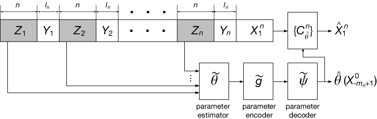
Let denote the composition of the parameter estimator and the parameter encoder, which we refer to as the first-stage encoder, and let denote the composition of the parameter decoder and the first-stage encoder. The decoder is the first-stage decoder. The collection defines the second-stage codes. The encoder and the decoder of are defined as
and
respectively. To assess the performance of , consider the function
The expectation of with respect to is precisely the Lagrangian performance of , at Lagrange multiplier , on the source . We consider separately the contributions of the first-stage and the second-stage codes. Define another function by
so that is the (random) Lagrangian performance of the code on . Hence,
so, taking expectations, we get
| (9) |
Our goal is to show that the first term in Eq. (9) converges to the th-order optimum , and that the second term is .
The proof itself is organized as follows. First we motivate the choice of the memory lengths in Section IV-B. Then we indicate how to select the database (Section IV-C) and how to implement the parameter estimator (Section IV-D) and the parameter encoder/decoder pair (Section IV-E). The proof is concluded by estimating the Lagrangian performance of the resulting code (Section IV-F) and the fidelity of the source identification at the decoder (Section IV-G). In the following, (in)equalities involving the relevant random variables are assumed to hold for all realizations and not just a.s., unless specified otherwise.
IV-B The memory length
Let , where is the common decay exponent of the -mixing coefficients in Condition 1, and let . We divide the -block into blocks of length interleaved by blocks of length (see Figure 1). The parameter estimator , although defined as acting on the entire , effectively will make use only of . The ’s are each distributed according to , but they are not independent. Thus, the set
is the effective memory of , and the effective memory length is .
Let denote the marginal distribution of , and let denote the product of copies of . We now show that we can approximate by in variational distance, increasingly finely with . Note that both and are defined on the -algebra , generated by all except those in , so that . Therefore, using induction and the definition of the -mixing coefficient (cf. Section II-A), we have
where the last equality follows from Condition 1 and from our choice of . This in turn implies the following useful fact (see also Lemma 4.1 of Yu [29]), which we shall heavily use in the proof: for any measurable function with ,
| (10) |
where the constant hidden in the notation depends on and on .
IV-C Construction of the database
The database, or the first-stage codebook, is constructed by random selection. Let be a probability distribution on which is absolutely continuous with respect to the Lebesgue measure and has an everywhere positive and continuous density . Let be a collection of independent random vectors taking values in , each generated according to independently of . We use to denote the process distribution of .
Note that the first-stage codebook is countably infinite, which means that, in principle, both the encoder and the decoder must have unbounded memory in order to store it. This difficulty can be circumvented by using synchronized random number generators at the encoder and at the decoder, so that the entries of can be generated as needed. Thus, by construction, the encoder will generate samples (where is the waiting time) and then communicate (a binary encoding of) to the decoder. Since the decoder’s random number generator is synchronized with that of the encoder’s, the decoder will be able to recover the required entry of .
IV-D Parameter estimation
The parameter estimator is constructed as follows. Because the source is stationary, it suffices to describe the action of on . In the notation of Section IV-A, let be the empirical distribution of . For every , define
where is the Yatracos class defined by the th-order densities (see Section III). Finally, define as any satisfying
where the extra term is there to ensure that at least one such exists. This is the so-called minimum-distance (MD) density estimator of Devroye and Lugosi [34, 35] (see also Devroye and Györfi [37]), adapted to the dependent-process setting of the present paper. The key property of the MD estimator is that
| (11) |
(see, e.g., Theorem 5.1 of Devroye and Györfi [37]). This holds regardless of whether the samples are independent or not.
IV-E Encoding and decoding of parameter estimates
Next we construct the parameter encoder-decoder pair . Given a , define the waiting time
with the standard convention that the infimum of the empty set is equal to . That is, given a , the parameter encoder looks through the codebook and finds the position of the first such that the variational distance between the th-order distributions and is at most . If no such is found, the encoder sets . We then define the maps and by
and
respectively. Thus, , and the bound
| (12) |
holds for every , regardless of whether is finite or infinite.
IV-F Performance of the code
Given the random codebook , the expected Lagrangian performance of our code on the source , is
| (13) |
We now upper-bound the two terms in (13). We start with the second term.
We need to bound the expectation of the waiting time . Our strategy borrows some elements from the paper of Kontoyiannis and Zhang [38]. Consider the probability
which is a random function of . From Condition 2, it follows for sufficiently large that
where . Because the density is everywhere positive, the latter probability is strictly positive for almost all , and so eventually almost surely. Thus, the waiting times will be finite eventually almost surely (with respect to both the source and the first-stage codebook ). Now, if , then, conditioned on , the waiting time is a geometric random variable with parameter , and it is not hard to show (see, e.g., Lemma 3 of Kontoyiannis and Zhang [38]) that for any
Setting , we have, for almost all , that
Then, by the Borel–Cantelli lemma,
eventually almost surely, so that
| (14) |
for almost every realization of the random codebook and for sufficiently large . We now obtain an asymptotic lower bound on . Define the events
Then by the triangle inequality we have
and, for sufficiently large, we can write
where (a) follows from the independence of and , (b) follows from the fact that the parameter estimator depends only on , and (c) follows from Condition 2 and the fact that . Since the density is everywhere positive and continuous at , for all for sufficiently large, so
| (15) |
where is the volume of the unit sphere in . Next, the fact that the minimum-distance estimate depends only on implies that the event belongs to the -algebra , and from (10) we get
| (16) |
Under , the -blocks are i.i.d. according to , and we can invoke the Vapnik–Chervonenkis machinery to lower-bound . In the notation of Sec. IV-D, define the event
Then implies by (11), and
| (17) |
where the second bound is by the Vapnik–Chervonenkis inequality (3) of Lemma II.1. Combining the bounds (16) and (17) and using Condition 1, we obtain
| (18) |
Now, if we choose
then the right-hand side of (18) can be further lower-bounded by . Combining this with (15), taking logarithms, and then taking expectations, we obtain
where is a constant that depends only on and . Using this and (14), we get that
for -almost every realization of the random codebook , for sufficiently large. Together with (12), this implies that
for -almost all realizations of the first-stage codebook.
We now turn to the first term in (13). Recall that, for each , the code is th-order optimal for . Using this fact together with the boundedness of the distortion measure , we can invoke Lemma A.3 in the Appendix and assume without loss of generality that each has a finite codebook (of size not exceeding ), and each codevector can be described by a binary string of no more than bits. Hence, . Let and be the marginal distributions of on and , respectively. Note that does not depend on . This, together with Condition 1 and the choice of , implies that
Furthermore,
where (a) follows by Fubini’s theorem and the boundedness of , while (b) follows from the definition of . The Lagrangian performance of the code , where , can be further bounded as
where (a) follows from Lemma A.3 in the Appendix, (b) follows from the th-order optimality of for , (c) follows, overbounding slightly, from the Lagrangian mismatch bound of Lemma A.2 in the Appendix, and (d) follows from the triangle inequality. Taking expectations, we obtain
| (19) |
The second term in (19) can be interpreted as the estimation error due to estimating by , while the first is the approximation error due to quantization of the parameter estimate . We examine the estimation error first. Using (11), we can write
| (20) |
Now, each is distributed according to , and we can approximate the expectation of with respect to by the expectation of with respect to the product measure :
where the second estimate follows from the Vapnik–Chervonenkis inequality (4) and from the choice of . This, together with (20), yields
| (21) |
As for the first term in (19), we have, by construction of the first-stage encoder, that
| (22) |
eventually almost surely, so the corresponding expectation is as well. Summing the estimates (21) and (22), we obtain
Finally, putting everything together, we see that, eventually,
| (23) |
for -almost every realization of the first-stage codebook . This proves (8), and hence (7).
IV-G Identification of the active source
We have seen that the expected variational distance between the -dimensional marginals of the true source and the estimated source converges to zero as . We wish to show that this convergence also holds eventually with probability one, i.e.,
| (24) |
-almost surely.
Given an , we have by the triangle inequality that implies
where is the minimum-distance estimate of from (cf. Section IV-E). Recalling our construction of the first-stage encoder, we see that this further implies
Finally, using the property (11) of the minimum-distance estimator, we obtain that
implies
Therefore,
| (25) | |||||
where (a) follows, as before, from the definition of the -mixing coefficient and (b) follows by the Vapnik–Chervonenkis inequality. Now, if we choose
for an arbitrary small , then (25) can be further upper-bounded by , which, owing to Condition 1 and the choice , is summable in . Thus,
and we obtain (24) by the Borel–Cantelli lemma.
V Examples
V-A Stationary memoryless sources
As a basic check, let us see how Theorem III.1 applies to stationary memoryless (i.i.d.) sources. Let , and let be the collection of all Gaussian i.i.d. processes, where
Then the -dimensional marginal for a given has the Gaussian density
with respect to the Lebesgue measure. This class of sources trivially satisfies Condition 1 with , and it remains to check Conditions 2 and 3.
To check Condition 2, let us examine the normalized th-order relative entropy between and , with and . Because the sources are i.i.d.,
Applying the inequality and some straightforward algebra, we get the bound
Now fix a small , and suppose that . Then , so we can further upper-bound by
Thus, for a given , we see that
for all in the open ball of radius around , with . Using Pinsker’s inequality, we have
for all . Thus, Condition 2 holds.
To check Condition 3, note that, for each , the Yatracos class consists of all sets of the form
| (26) |
for all . Let and . Then we can rewrite (26) as
This is the set of all such that
where is a third-degree polynomial in the six parameters . It then follows from Lemma II.2 that is a VC class with . Therefore, Condition 3 holds as well.
V-B Autoregressive sources
Again, let and consider the case when is a Gaussian autoregressive source of order , i.e., it is the output of an autoregressive filter of order driven by white Gaussian noise. Then there exist real parameters (the filter coefficients), such that
where is an i.i.d. Gaussian process with zero mean and unit variance. Let be the set of all , such that the roots of the polynomial , where , lie outside the unit circle in the complex plane. This ensures that is a stationary process. We now proceed to check that Conditions 1–3 of Section III are satisfied.
The distribution of each is absolutely continuous, and we can invoke the result of Mokkadem [31] to conclude that, for each , the process is geometrically mixing, i.e., for every , there exists some , such that . Now, for any fixed , for sufficiently large, so Condition 1 holds.
To check Condition 2, note that, for each , the Fisher information matrix is independent of (see, e.g., Section 6 of Klein and Spreij [39]). Thus, the asymptotic Fisher information matrix exists and is nonsingular [39, Theorem 6.1], so, recalling the discussion in Section III, we conclude that Condition 2 holds also.
To verify Condition 3, consider the -dimensional marginal , which has the Gaussian density
where is the th-order autocorrelation matrix of . Thus, the Yatracos class consists of sets of the form
for all . Now, for every , let . Since is uniquely determined by , we have for all . Using this fact, as well as the easily established fact that the entries of the inverse covariance matrix are second-degree polynomials in the filter coefficients , we see that, for each , the condition can be expressed as , where is quadratic in the real variables . Thus, we can apply Lemma II.2 to conclude that . Therefore, Condition 3 is satisfied as well.
V-C Hidden Markov processes
A hidden Markov process (or a hidden Markov model, see, e.g., [40]) is a discrete-time bivariate random process , where is a homogeneous Markov chain and is a sequence of random variables which are conditionally independent given , and the conditional distribution of is time-invariant and depends on only through . The Markov chain , also called the regime, is not available for observation. The observable component is the source of interest. In information theory (see, e.g., [41] and references therein), a hidden Markov process is a discrete-time finite-state homogeneous Markov chain , observed through a discrete-time memoryless channel, so that is the observation sequence at the output of the channel.
Let denote the number of states of . We assume without loss of generality that the state space of is the set . Let denote the transition matrix of , where . If is ergodic (i.e., irreducible and aperiodic), then there exists a unique probability distribution on such that (the stationary distribution of ), see, e.g., Section 8 of Billingsley [42]. Because in this paper we deal with two-sided random processes, we assume that has been initialized with its stationary distribution at some time sufficiently far away in the past, and can therefore be thought of as a two-sided stationary process. Now consider a discrete-time memoryless channel with input alphabet and output (observation) alphabet for some . It is specified by a set of transition densities (with respect to , the Lebesgue measure on ). The channel output sequence is the source of interest.
Let us take as the parameter space the set of all transition matrices , such that all for some fixed . For each and each , the density is given by
where for every . We assume that the channel transition densities , are fixed a priori, and do not include them in the parametric description of the sources. We do require, though, that
and
We now proceed to verify that Conditions 1–3 of Section III are met.
Let denote the -step transition probability for states . The positivity of implies that the Markov chain is geometrically ergodic, i.e.,
| (27) |
where and , see Theorem 8.9 of Billingsley [42]. Note that (27) implies that
This in turn implies that the sequence is exponentially -mixing, see Theorem 3.10 of Vidyasagar [24]. Now, one can show (see Section 3.5.3 of Vidyasagar [24]) that there exists a measurable mapping , such that , where is an i.i.d. sequence of random variables distributed uniformly on , independently of . It is not hard to show that, if is exponentially -mixing, then so is the bivariate process . Finally, because is given by a time-invariant deterministic function of , the -mixing coefficients of are bounded by the corresponding -mixing coefficients of , and so is exponentially -mixing as well. Thus, for each , there exists a , such that , and consequently Condition 1 holds.
To show that Condition 2 holds, we again examine the asymptotic behavior of the Fisher information matrix as . Under our assumptions on the state transition matrices in and on the channel transition densities , we can invoke the results of Section 6.2 in Douc, Moulines and Rydén [43] to conclude that the asymptotic Fisher information matrix exists (though it is not necessarily nonsingular). Thus, Condition 2 is satisfied.
Finally we check Condition 3. The Yatracos class consists of all sets of the form
for all . The condition can be written as , where for each , is a polynomial of degree in the parameters , . Thus, Lemma II.2 implies that , so Condition 3 is satisfied as well.
VI Conclusions and future directions
We have shown that, given a parametric family of stationary mixing sources satisfying some regularity conditions, there exists a universal scheme for joint lossy compression and source identification, with the th-order Lagrangian redundancy and the variational distance between -dimensional marginals of the true and the estimated source both converging to zero as , as the block length tends to infinity. The sequence quantifies the learnability of the -dimensional marginals. This generalizes our previous results from [9, 10] for i.i.d. sources.
We can outline some directions for future research.
- •
Both in our earlier work [9, 10] and in the present paper, we assume that the dimension of the parameter space is known a priori. It would be of interest to consider the case when the parameter space is finite-dimensional, but its dimension is not known. Thus, we would have a hierarchical model class , where, for each , is an open subset of , and we could use a complexity regularization technique, such as “structural risk minimization” (see, e.g., Lugosi and Zeger [44] or Chapter 6 of Vapnik [22]), to adaptively trade off the estimation and the approximation errors.
- •
The minimum-distance density estimator of Devroye and Lugosi [34, 35], which plays the key role in our scheme both here and in [9, 10], is not easy to implement in practice, especially for multidimensional alphabets. On the other hand, there are two-stage universal schemes, such as that of Chou, Effros and Gray [14], which do not require memory and select the second-stage code based on pointwise, rather than average, behavior of the source. These schemes, however, are geared toward compression, and do not emphasize identification. It would be worthwhile to devise practically implementable universal schemes that strike a reasonable compromise between these two objectives.
- •
Finally, neither here nor in our earlier work [9, 10] have we considered the issues of optimality. It would be of interest to obtain lower bounds on the performance of any universal scheme for joint lossy compression and identification, say, in the spirit of minimax lower bounds in statistical learning theory (cf., e.g., Chapter 14 of Devroye, Györfi and Lugosi [21]).
Conceptually, our results indicate that links between statistical modeling (parameter estimation) and universal source coding, exploited in the lossless case by Rissanen [2, 3], are present in the domain of lossy coding as well. We should also mention that another modeling-based approach to universal lossy source coding, due to Kontoyiannis and others (see, e.g., Madiman and Kontoyiannis [45] and references therein), treats code selection as a statistical estimation problem over a class of model distributions in the reproduction space. This approach, while closer in spirit to Rissanen’s Minimum Description Length (MDL) principle [46], does not address the problem of joint source coding and identification, but it provides a complementary perspective on the connections between lossy source coding and statistical modeling.
Appendix A Properties of Lagrange-optimal variable-rate quantizers
In this Appendix, we detail some properties of Lagrange-optimal variable-rate vector quantizers. Our exposition is patterned on the work of Linder [19], with appropriate modifications.
As elsewhere in the paper, let be the source alphabet and the reproduction alphabet, both assumed to be Polish spaces. As before, let the distortion function be induced by a -bounded metric on a Polish metric space containing . For every , define the metric on by
For any pair of probability measures on , let be the set of all probability measures on having and as marginals, and define the Wasserstein metric
(See Gray, Neuhoff and Shields [47] for more details and applications.) Note that, because is a bounded metric,
for all . Taking the infimum of both sides over all and observing that
see, e.g., Section I.5 of Lindvall [48], we get the useful bound
| (A.1) |
Now, for each , let denote the set of all discrete probability distributions on with finite entropy. That is, if and only if it is concentrated on a finite or a countable set , and
For every , consider the set of all one-to-one maps , such that, for each , the collection satisfies the Kraft inequality, and let
be the minimum expected code length. Since the entropy of is finite, there is always a minimizing , and the Shannon–Fano bound (see Section 5.4 of Cover and Thomas [1]) guarantees that .
Now, for any , any probability distribution on , and any , define
To give an intuitive meaning to , let and be jointly distributed random variables with and , such that their joint distribution achieves . Then is the expected Lagrangian performance, at Lagrange multiplier , of a stochastic variable-rate quantizer which encodes each point as a binary codeword with length and decodes it to in the support of with probability .
The following lemma shows that deterministic quantizers are as good as random ones:
Lemma A.1
Let be the expected Lagrangian performance of an -block variable rate quantizer operating on , and let be the expected Lagrangian performance, with respect to , of the best -block variable-rate quantizer. Then
Proof:
Consider any quantizer with . Let be the distribution of . Clearly, , and
Hence, . To prove the reverse inequality, suppose that and achieve for some . Let be their joint distribution. Let be the support of , let achieve , and let be the associated binary code. Define the quantizer by φ(s) = y_i if s = c^*_Q(i) and f(x^n) = arg min _s ∈S (ρ_n(x^n,φ(s)) + λℓ_n(s)). Then L_P(C^n,λ) = E _P { min_s ∈S (ρ_n(X^n,φ(s)) + λℓ_n(s))}. On the other hand,
so that , and the lemma is proved. ∎
The following lemma gives a useful upper bound on the Lagrangian mismatch:
Lemma A.2
Let be probability distributions on . Then
Proof:
Suppose . Let achieve (or be arbitrarily close). Then
where in (a) we used Lemma A.1) in (b) we used the definition of , in (c) we used the fact that is a metric and the triangle inequality, and in (d) we used the bound (A.1). ∎
Finally, the lemma below shows that, for bounded distortion functions, Lagrange-optimal quantizers have finite codebooks:
Lemma A.3
For positive integers , let denote the set of all zero-memory variable-rate quantizers with block length , such that for every , the associated binary code of satisfies and for every . Let be a probability distribution on . Then
with and .
Proof:
Let with encoder and decoder achieve the th-order optimum for . Let be the shortest binary string in , i.e., ℓ(s_0) = min_s ∈Sℓ(s). Without loss of generality, we can take as the minimum-distortion encoder, i.e., f_*(x^n) = arg min _s ∈S (ρ_n(x^n,φ_*(s)) + λℓ_n(s)). Thus, for any and any , ρ_n(x^n,φ_*(s)) + λℓ_n(s) ≤ρ_n(x^n,φ_*(s_0)) + λℓ_n(s_0). Hence, for all . Furthermore, .
Now pick an arbitrary reproduction string , let be the empty binary string (of length zero), and let be the zero-rate quantizer with the constant encoder and the decoder . Then . On the other hand, . Therefore, λℓ_n(s_0) ≤L_P(C^n_*,λ) ≤L_P(C^n_0,λ) ≤ρ_max, so that . Hence, ℓ(s) ≤2nρ_max/λ, ∀s∈S, Since the strings in must satisfy Kraft’s inequality, we have 1 ≥∑_s ∈S 2^-ℓ(s) ≥—S—2^-2nρ_max/λ, which implies that . ∎
Acknowledgment
The author would like to thank Andrew R. Barron, Ioannis Kontoyiannis and Mokshay Madiman for stimulating discussions, and the anonymous reviewers for several useful suggestions that helped improve the paper.
References
- [1] T. M. Cover and J. A. Thomas, Elements of Information Theory. New York: Wiley, 1991.
- [2] J. Rissanen, “Universal coding, information, prediction, and estimation,” IEEE Trans. Inform. Theory, vol. IT-30, no. 4, pp. 629–636, July 1984.
- [3] ——, “Fisher information and stochastic complexity,” IEEE Trans. Inform. Theory, vol. 42, no. 1, pp. 40–47, January 1996.
- [4] J. Ziv and A. Lempel, “Compression of individual sequences by variable-rate coding,” IEEE Trans. Inform. Theory, vol. IT-24, pp. 530–536, September 1978.
- [5] J. C. Kieffer, “Strongly consistent code-based identification and order estimation for constrained finite-state model classes,” IEEE Trans. Inform. Theory, vol. 39, no. 3, pp. 893–902, May 1993.
- [6] N. Merhav, “Bounds on achievable convergence rates of parameter estimation via universal coding,” IEEE Trans. Inform. Theory, vol. 40, no. 4, pp. 1210–1215, July 1994.
- [7] T. Weissman and E. Ordentlich, “The empirical distribution of rate-constrained source codes,” IEEE Trans. Inform. Theory, vol. 51, no. 11, pp. 3718–3733, November 2005.
- [8] G. Tao, Adaptive Control Design and Analysis. Hoboken: Wiley, 2003.
- [9] M. Raginsky, “Joint fixed-rate universal lossy coding and identification of continuous-alphabet memoryless sources,” IEEE Trans. Inform. Theory, vol. 54, no. 7, pp. 3059–3077, July 2008.
- [10] ——, “Joint universal lossy coding and identification of i.i.d. vector sources,” in Proc. IEEE Int. Symp. on Information Theory, Seattle, July 2006, pp. 577–581.
- [11] E.-H. Yang and Z. Zhang, “On the redundancy of lossy source coding with abstract alphabets,” IEEE Trans. Inform. Theory, vol. 45, no. 4, pp. 1092–1110, May 1999.
- [12] V. N. Vapnik and A. Y. Chervonenkis, “On the uniform convergence of relative frequencies of events to their probabilities,” Theory Probab. Appl., vol. 16, pp. 264–280, 1971.
- [13] P. A. Chou, T. Lookabaugh, and R. M. Gray, “Entropy-constrained vector quantization,” IEEE Trans. Acoust. Speech Signal Processing, vol. 37, no. 1, pp. 31–42, January 1989.
- [14] P. A. Chou, M. Effros, and R. M. Gray, “A vector quantization approach to universal noiseless coding and quantization,” IEEE Trans. Inform. Theory, vol. 42, no. 4, pp. 1109–1138, July 1996.
- [15] R. M. Gray, Entropy and Information Theory. New York: Springer-Verlag, 1990.
- [16] V. A. Volkonskii and Y. A. Rozanov, “Some limit theorems for random functions, I,” Theory Probab. Appl., vol. 4, pp. 178–197, 1959.
- [17] ——, “Some limit theorems for random functions, II,” Theory Probab. Appl., vol. 6, pp. 186–198, 1961.
- [18] D. L. Neuhoff and R. K. Gilbert, “Causal source codes,” IEEE Trans. Inform. Theory, vol. IT-28, no. 5, pp. 701–713, September 1982.
- [19] T. Linder, “Learning-theoretic methods in vector quantization,” in Principles of Nonparametric Learning, L. Györfi, Ed. New York: Springer-Verlag, 2001.
- [20] M. Effros, P. A. Chou, and R. M. Gray, “Variable-rate source coding theorems for stationary nonergodic sources,” IEEE Trans. Inform. Theory, vol. 40, no. 6, pp. 1920–1925, November 1994.
- [21] L. Devroye, L. Györfi, and G. Lugosi, A Probabilistic Theory of Pattern Recognition. New York: Springer-Verlag, 1996.
- [22] V. N. Vapnik, Statistical Learning Theory. New York: Wiley, 1998.
- [23] L. Devroye and G. Lugosi, Combinatorial Methods in Density Estimation. New York: Springer-Verlag, 2001.
- [24] M. Vidyasagar, Learning and Generalization, 2nd ed. London: Springer-Verlag, 2003.
- [25] N. Sauer, “On the density of families of sets,” J. Combin. Theory Ser. A, vol. 13, pp. 145–147, 1972.
- [26] R. M. Dudley, “Central limit theorems for empirical measures,” Ann. Probab., vol. 6, pp. 898–929, 1978.
- [27] M. Karpinski and A. Macintyre, “Polynomial bounds for VC dimension of sigmoidal and general Pfaffian neural networks,” J. Comput. Sys. Sci., vol. 54, pp. 169–176, 1997.
- [28] S. N. Bernstein, “Sur l’extension du théorème limite du calcul des probabilités aux sommes de quantités dependantes,” Math. Ann., vol. 97, pp. 1–59, 1927.
- [29] B. Yu, “Rates of convergence for empirical processes of stationary mixing sequences,” Ann. Probab., vol. 22, no. 1, pp. 94–116, 1994.
- [30] R. Meir, “Nonparametric time series prediction through adaptive model selection,” Machine Learning, vol. 39, pp. 5–34, 2000.
- [31] A. Mokkadem, “Mixing properties of ARMA processes,” Stochastic Process. Appl., vol. 29, pp. 309–315, 1988.
- [32] B. S. Clarke and A. R. Barron, “Information-theoretic asymptotics of Bayes methods,” IEEE Trans. Inform. Theory, vol. 36, no. 3, pp. 453–471, May 1990.
- [33] Y. G. Yatracos, “Rates of convergence of minimum distance estimates and Kolmogorov’s entropy,” Ann. Math. Statist., vol. 13, pp. 768–774, 1985.
- [34] L. Devroye and G. Lugosi, “A universally acceptable smoothing factor for kernel density estimation,” Ann. Statist., vol. 24, pp. 2499–2512, 1996.
- [35] ——, “Nonasymptotic universal smoothing factors, kernel complexity and Yatracos classes,” Ann. Statist., vol. 25, pp. 2626–2637, 1997.
- [36] P. Elias, “Universal codeword sets and representations of the integers,” IEEE Trans. Inform. Theory, vol. IT-21, no. 2, pp. 194–203, March 1975.
- [37] L. Devroye and L. Györfi, “Distribution and density estimation,” in Principles of Nonparametric Learning, L. Györfi, Ed. New York: Springer-Verlag, 2001.
- [38] I. Kontoyiannis and J. Zhang, “Arbitrary source models and Bayesian codebooks in rate-distortion theory,” IEEE Trans. Inform. Theory, vol. 48, no. 8, pp. 2276–2290, August 2002.
- [39] A. Klein and P. Spreij, “The Bezoutian, state space realizations and Fisher’s information matrix of an ARMA process,” Lin. Algebra Appl., vol. 416, pp. 160–174, 2006.
- [40] P. J. Bickel, Y. Ritov, and T. Rydén, “Asymptotic normality of the maximum-likelihood estimator for general hidden Markov models,” Ann. Statist., vol. 26, no. 4, pp. 1614–1635, 1997.
- [41] Y. Ephraim and N. Merhav, “Hidden Markov processes,” IEEE Trans. Inform. Theory, vol. 48, no. 6, pp. 1518–1569, June 2002.
- [42] P. Billingsley, Probability and Measure, 3rd ed. Wiley, New York.
- [43] R. Douc, É. Moulines, and T. Rydén, “Asymptotic properties of the maximum likelihood estimator in autoregressive models with Markov regime,” Ann. Statist., vol. 32, no. 5, pp. 2254–2304, 2004.
- [44] G. Lugosi and K. Zeger, “Concept learning using complexity regularization,” IEEE Trans. Inform. Theory, vol. 42, no. 1, pp. 48–54, January 1996.
- [45] M. Madiman and I. Kontoyiannis, “Second-order properties of lossy likelihoods and the MLE/MDL dichotomy in lossy compression,” Brown University, APPTS Report No. 04-5, May 2004, available [Online] at http://www.dam.brown.edu/ptg/REPORTS/04-5.pdf.
- [46] A. Barron, J. Rissanen, and B. Yu, “Minimum description length principle in coding and modeling,” IEEE Trans. Inform. Theory, vol. 44, no. 6, pp. 2743–2760, October 1998.
- [47] R. M. Gray, D. L. Neuhoff, and P. S. Shields, “A generalization of Ornstein’s distance with applications to information theory,” Ann. Probab., vol. 3, no. 2, pp. 315–328, 1975.
- [48] T. Lindvall, Lectures on the Coupling Method. New York: Dover, 2002.