Approximation of target problems in Blackwell spaces

Giacomo Aletti^?? abel=u1 url]http://www.mat.unimi.it/ aletti Diane Saada^??

On a weakly Blackwell space we show how to define a Markov chain approximating problem, for the target problem. The approximating problem is proved to converge to the optimal reduced problem under different pseudometrics. A computational example of compression of information is discussed.

University of Milan^?? and The Hebrew University of Jerusalem^??

Let $X_{n}$ be an homogeneous Markov chain. Suppose the process stops once it reaches an absorbing class, called the target, according to a given stopping rule: the resulting problem is called target problem (TP). The idea is to reduce the available information in order to only use the necessary information which is relevant with respect to the target. A new Markov chain, associated with a new equivalent but reduced matrix is defined. In the (large) finite case, the problem has been solved for TPs: in [1, 2, 3], it has been proved that any TP on a finite set of states has its “best target” equivalent Markov chain. Moreover, this chain is unique and there exists a polynomial time algorithm to reach this optimum.

The question is now to find, in generality, an $\epsilon$ –approximation of the Markov problem when the state space is measurable. The idea is to merge into one group the points that $\epsilon$ -behave the same with respect to the objective, but also in order to keep an almost equivalent Markov chain, with respect to the other “groups”. The construction of these groups is done through equivalence relations and hence each group corresponds to a class of equivalence. In fact, there are many other mathematical fields where approximation problems are faced by equivalences. For instance, in integration theory, we use simple functions, in functional analysis, we use the density of countable generated subspaces and in numerical analysis, we use the finite elements method.

In this paper, the approximation is made by means of discrete equivalences, which will be defined in the following. The purpose of any approximation is to reach the exact solution when $\epsilon\rightarrow 0$ . We prove that the sequence of approximations tends to the optimal exact equivalence relation defined in [1, 2, 3], when we refine the groups. Finer equivalence will imply better approximation, and accordingly the limit will be defined as a countably generated equivalence.

Under a very general Blackwell type hypothesis on the measurable space, we show that it is equivalent to speak on countably generated equivalence relationships or on measurable real functions on the measurable space of states. If we do not work under this framework of Blackwell spaces, we can be faced to paradoxes, as it is explained by [6], of enlarging $\sigma$ –algebras, while decreasing the information available to a decision-maker. The $\epsilon$ –approximation of the Markov chain depends always upon the kind of objective. In [9], Jerrum deals with ergodic Markov chains. His objective is to approximate the stationary distribution by means of a discrete approximating Markov chain, whose limit distribution is close in a certain sense to the original one. However, unlike our following work, his purpose is not the explicit and unified construction of the approximating process. In this paper, we focus on the target problem. We solve extensively the TP, where the objective is connected with the conditional probability of reaching the target $T$ , namely $\mathbb{P}(X_{n}\in T|X_{0}=x)$ , for any $n,x$ . This part extends the work in [1, 2, 3], since TPs’ approximation may help to understand the behavior of those TPs where the best equivalent Markov chain is also very large. The setting of an approximating problem can be extended to a general form, but we will not develop it in this paper.

1 Main results

Let $(X,\mathcal{X})$ be a measurable space. We equip it with an Assumption (A0) that will be explained when required. Let $P$ be any transition probability on $(X,\mathcal{X})$ . An homogeneous Markov process $(X_{n})_{n}$ is naturally associated to $(X,\mathcal{X},P)$ . In the target problem, we are interested in the probabilities of reaching the target class $T$ within $n$ steps, namely in

\mathbb{P}\big(\{X_{n}\in T\}\big|X_{0}=x\big)\qquad\text{for any $n$ and $x$}.

The set $T$ is a priori given and does not change through the computations.

Definition 1.

Let $(X,\mathcal{X})$ be a measurable space and let $T\in{\mathcal{X}}$ . Let ${\mathcal{F}}\subseteq{\mathcal{X}}$ be a sub $\sigma$ -algebra of $\mathcal{X}$ such that $T\in{\mathcal{F}}$ . A function $P:X\times{\mathcal{F}}\rightarrow[0,1]$ is a transition probability on $(X,\mathcal{F})$ if

•

$P(x,\cdot)$ is a probability measure on ${\mathcal{F}}$ , for any $x\in X$ ;
•

$P(\cdot,F)$ is ${\mathcal{F}}$ -measurable, for any $F\in{\mathcal{F}}$ .

Given a transition probability $P$ on $(X,\mathcal{F})$ , we denote by $P^{n}$ the transition probability on $(X,\mathcal{F})$ given inductively by

P^{1}=P;\qquad P^{n+1}(x,F)=\int_{X}P(x,dy)P^{n}(y,F)

We denote by $\mathrm{TrP}(X,\mathcal{X},\mathcal{F})$ the set of the transition probabilities on $(X,\mathcal{F})$ . We denote by ${\mathbb{TP}}_{X}=\cup_{\mathcal{F}\subseteq\mathcal{X}}\mathrm{TrP}(X,\mathcal{X},\mathcal{F})$ the set of all transition probabilities on $X$ , that we equip with a suitable pseudometric $d$

d(P_{1},P_{2})=\sup_{x}\sum_{n}\beta^{n}\big|P_{1}^{n}(x,T)-P_{2}^{n}(x,T)\big|.

It is such that

d(P_{1},P_{2})=0\qquad\Longleftrightarrow\qquad P_{1}^{n}(x,T)=P_{2}^{n}(x,T),\quad\text{for any $n$ and $x$}.

This pseudo-metric is obviously compatible with the target $T$ and appears as a loss function of using $P_{2}$ instead of $P_{1}$ , whatever is the initial point $x$ ( $\beta\in(0,1)$ is a discount rate). The point will be, with no surprise, to let this distance go to $0$ .

A target problem is defined through a transition probability $P\in({\mathbb{TP}}_{X},d)$ .

Definition 2.

A target problem is a quadruple $(X,{\mathcal{F}},T,P)$ , where $P\in\mathrm{TrP}(X,\mathcal{X},\mathcal{F})$ and $T\in\mathcal{F}$ . A simple target problem is a target problem where ${\mathcal{F}}$ is generated by an at most countable partition of $X$ .

The main purpose of this paper is to approximate any target problem with a sequence of simple target problems in the spirit of the construction the Lebesgue integral, where the integral of a function $f$ is approximated by the integral of simple functions $f_{n}=\sum_{i}c_{i}I_{C_{i}}$ . The Lebesgue approximation requires at each step $n\in\mathbb{N}$ two choices: the choice of the subdivision $(C_{i})_{i}$ and the choice of the function values $(c_{i})_{i}$ on each subdivision.

Definition 3.

We call strategy $\mathrm{Str}$ a sequence of maps $({\mathrm{Str}}_{n})_{n}$ from the set of the target problems to the set of the simple target problems.

In the “Lebesgue example” given above, the strategy is related to the “objective” of the problem (the integral) and the pseudometric $d(f,f_{n})=\int|f-f_{n}|dx$ is required to go to $0$ as $n$ goes to infinity. Here also, a strategy is meaningful if $d(P,{\mathrm{Str}}_{n}(P))$ tends to $0$ as $n$ goes to infinity. Moreover, for what concerns applications, given a target problem $(X,\mathcal{X},T,P)$ a good strategy should not need the computation of $P^{n}$ , $n>1$ . The first main result of this paper is the existence of a class of good strategies, called target algorithms.

Theorem 1.

For any target problem $(X,\mathcal{F},T,P)$ and any target algorithm $\mathrm{Str}$ ,

\lim_{n\to\infty}d(P,P_{n})=0,

where $(X,{\mathcal{F}}_{n},T,P_{n})={\mathrm{Str}}_{n}(X,{\mathcal{F}},T,P)$ .

Two questions immediately arise: does the sequence $({\mathrm{Str}}_{n}(P))_{n}$ have a limit (and in which sense)? Moreover, since $d$ is defined as a pseudometric, does this limit depend on the choice of $\mathrm{Str}$ ?

The extension of the concept of compatible projection given in [3, 1, 2] to our framework will enable us to understand better the answer to these questions. A measurable set $A\neq\emptyset$ of a measurable space $(X,\mathcal{X})$ is an $\mathcal{X}$ -atom if it has no non-empty measurable proper subset. No two distinct atoms intersect. If the $\sigma$ -field is countably generated, say by the sequence $\{A_{n}\}$ then the atoms of $\mathcal{X}$ are of the form $\cap_{n}C_{n}$ where each $C_{n}$ is either $A_{n}$ or $X\setminus A_{n}$ .

Definition 4.

An equivalence relationship $\pi$ on a measurable set $(X,\mathcal{X})$ is measurable (discrete) if there exists a (discrete) random variable $f:(X,\mathcal{X})\to(\mathbb{R},\mathcal{B}_{\mathbb{R}})$ ( $\mathcal{B}_{\mathbb{R}}$ denotes the Borel $\sigma$ -algebra), such that

x\,\pi\,y\qquad\Longleftrightarrow\qquad f(x)=f(y),

and we denote it by $\pi=\pi_{f}$ . Let $(X,{\mathcal{F}},T,P)$ be a target problem. A compatible projection is a measurable equivalency $\pi_{f}$ such that

P(x,F)=P(y,F),\qquad\forall x\,\pi_{f}\,y,\forall F\in\sigma(f).

(1)

A compatible projection $\pi$ is said to be optimal if $\pi\supseteq\pi^{\prime}$ , for any other compatible projection $\pi^{\prime}$ .

Remark 1.

This definition is well posed if

\pi_{f}=\pi_{g}\Longleftrightarrow\sigma(f)=\sigma(g).

Assumption (A0) ensures that the definition of measurable equivalency is indeed well posed. This assumption will be stated and discussed in Section 4.

Theorem 2.

If $\pi=\pi_{f}$ is a compatible projection for the target problem $(X,{\mathcal{F}},T,P)$ , then there exists a target problem $(X,\sigma(f),T,P_{\pi})$ . such that $P_{\pi}(x,F)=P(x,F)$ for any $F\in\sigma(f)$ .

It is not said “a priori” that an optimal compatible projection must exist. If it is the case, then this equivalence is obviously unique.

Theorem 3.

For any target problem $(X,\mathcal{F},T,P)$ , there exists a (unique) optimal compatible projection $\pi$ .

To conclude the main results, let us first come back to the Lebesgue example. The simple function $f_{n}=\sum_{i}c_{i}I_{C_{i}}$ are chosen so that $\sigma(C_{n})$ increases to $\sigma(f)$ and $f_{n}(x)\to f(x)$ . The following theorem guarantees these two facts by showing the “convergence” of any strategy to the optimal problem.

Theorem 4.

Let ${\mathrm{Str}}_{n}(X,{\mathcal{F}},T,P)=(X,{\mathcal{F}}_{n},T,P_{n})$ , with $\mathrm{Str}$ target algorithm and let $\pi$ be the optimal compatible projection associated to the target problem $(X,{\mathcal{F}},T,P)$ . Then

•

${\mathcal{F}}_{n}\subseteq{\mathcal{F}}_{n+1}$ for any $n$ , and $\vee_{n}{\mathcal{F}}_{n}={\mathcal{F}}_{\pi}$ ;
•

$\lim_{n}P_{n}(x,F)=P_{\pi}(x,F)$ , for any $F\in\cup_{m}{\mathcal{F}}_{m}$ .

Remark 2 (The topology $\mathrm{Top}$ ).

In Theorems 1–4, we have proved the convergence of $({P}_{n})_{n}$ to $P_{\pi}$ with respect to the pseudometric $d$ . The pseudometric topology $\mathrm{Top}$ is the topology induced by the open balls $B_{r}(P)=\{Q\in{\mathbb{TP}}_{X}\colon d(P,Q)<r\}$ , which form a basis for the topology. Accordingly, the previous theorems may be reread in terms of convergence of $P_{n}$ to $P$ on the topological space $({\mathbb{TP}}_{X},\mathrm{Top})$ .

1.1 Connection with weak convergence

Given a strategy $(X,{\mathcal{F}}_{n},T,P_{n})_{n}$ , if we want to show a sort of weak convergence of $P_{n}(x,\cdot)$ to $P(x,\cdot)$ , for any $x$ , we face the two following problems

•

each $P_{n}(x,\cdot)$ is defined on a different domain (namely, on $\mathcal{F}_{n}$ );
•

we did not have required a topology on $X$ .

First, we want to introduce a new definition of probability convergence which takes into account the first restriction. The idea is given in the following example.

Example 1.

Let $\mathcal{F}_{n}=\sigma(\{(i2^{-n},(i+1)2^{-n}],i=0,\ldots,2^{n}-1\})$ be the $\sigma$ -algebra on $(0,1]$ generated by the dyadic subdivision. Suppose we know that $\nu_{n}:\mathcal{F}_{n}\to[0,1]$ is the unique probability on $\mathcal{F}_{n}$ s.t. for any $i$ , $\nu_{n}((i2^{-n},(i+1)2^{-n}])=2^{-n}$ . Even if $\nu_{n}$ is not defined on the Borel sets of $(0,1]$ , it is clear that in “some” sense, it must happen that $\nu_{n}\to\nu_{*}$ , where $\nu_{*}$ is the Lebesgue measure on the Borel sets of $(0,1]$ . Note that the cumulative function of ${\nu}_{n}$ is not defined, and therefore a standard weak convergence cannot be verified.

In fact, we know that

\nu_{n}\Big(\big(-\infty,\frac{i}{2^{n}}\big]\Big)=\nu_{n}\Big(\big(0,\frac{i}{2^{n}}\big]\Big)=\frac{i}{2^{n}},

(2)

i.e., in this case, as $n\to\infty$ , we can determine the cumulative function in a dense subset. This fact allows to hope that $\nu_{n}\to\nu_{*}$ in a particular sense.

Definition 5.

Let $(X,\mathcal{X},(\mathcal{X}_{n})_{n})$ be a filtered space, and set ${\mathcal{X}}_{\infty}=\vee_{n}{\mathcal{X}}_{n}$ . Let $\nu_{n}:{\mathcal{X}}_{n}\rightarrow[0,1]$ , $n\geq 1$ and $\nu_{\infty}:{\mathcal{X}}_{\infty}\rightarrow[0,1]$ be probability measures. We say that $\nu_{n}$ converges totally to $\nu_{\infty}$ on the topological space $(X,\tau)$ as $n$ tends to infinity, if $\bar{\nu}_{n}\mathop{\longrightarrow}\limits^{w}_{\tau}\nu_{\infty}$ (converges in weak sense on $(X,\tau)$ ), for any $\bar{\nu}_{n}:{\mathcal{X}}_{\infty}\rightarrow[0,1]$ , such that ${\bar{\nu}_{n}}{}_{|_{{\mathcal{X}}_{n}}}=\nu_{n}$ . We write $\nu_{n}\mathop{\longrightarrow}\limits^{\mathrm{tot}}_{\tau}\nu_{\infty}$ .

Going back to the example, it is simple to check that $\nu_{n}\mathop{\longrightarrow}\limits^{\mathrm{tot}}_{\tau(0,1]}\nu_{*}$ , where $\nu_{n},\nu_{*}$ are given in Example 1 and $\tau(0,1]$ is the standard topology on $(0,1]$ . In fact, let $(\bar{\nu}_{n})_{n}$ be any extension of $({\nu}_{n})_{n}$ to the Borel sets of $(0,1]$ . For any $t\in(0,1)$ , we have by (2) that

t-\frac{1}{2^{n}}\leq F_{\bar{\nu}_{n}}(t)\leq t+\frac{1}{2^{n}},

where $F_{\bar{\nu}_{n}}$ is the cumulative function of $\bar{\nu}_{n}$ , which implies the weak convergence of $\bar{\nu}_{n}$ to $\nu_{*}$ and, therefore, ${\nu}_{n}\mathop{\longrightarrow}\limits^{\mathrm{tot}}_{\tau(0,1]}\nu_{*}$ .

For what concerns the topology on $X$ , we will define the topological space $(X,\varrho_{P})$ induced by the pseudometric $d_{P}$ associated to the target problem $(X,{\mathcal{F}},T,P)$ , and the pseudometric $d$ . In this way $\varrho_{P}$ is defined only with the data of the problem. One may ask: is this topology too poor? The answer is no, since it is defined by the interesting pseudometric $d_{P}$ . In fact, $d_{P}(x,y)<\epsilon$ means that $x$ and $y$ play “almost the same role” with respect to $T$ . A direct algorithm which takes $d_{P}$ into account needs the computation of $P^{n}$ at each step. In any case, even if $d_{P}$ may not be computable, it defines a nontrivial interesting topology $\varrho_{P}$ on $X$ . As expected, we have the following theorem.

Theorem 5.

Let ${\mathrm{Str}}_{n}(X,{\mathcal{F}},T,P)=(X,{\mathcal{F}}_{n},T,P_{n})$ , with $\mathrm{Str}$ target algorithm. Then

P_{n}\mathop{\longrightarrow}\limits^{\mathrm{tot}}_{\varrho_{P}}P.

2 The target algorithm

In this section, we introduce the core of the approximating target problem, namely a set of strategies $\mathrm{Str}$ which solves the target problem.

Given a measurable space $(X,\mathcal{X})$ and a target problem $(X,\mathcal{F},T,P)$ , the target algorithm is built in the spirit of the exact one given in [1, 2], which starts from the largest classes $T$ and $X\setminus T$ and then reaches the optimal classes according to a backward construction.

The target algorithm defines a strategy $\mathrm{Str}=(\mathrm{Str}_{n})_{n}$ , where

\mathrm{Str}_{n}(X,\mathcal{F},T,P)=(X,\mathcal{F}_{n},T,P_{n}),

and it consists of three steps:

1.

the choice of a sequence $(\sim_{\epsilon_{n}})_{n}$ of equivalences on the simplex on the unit ball of $\ell_{1}$ with $\epsilon_{n}\to 0$ ;
2.

the definition of a filtration $(\mathcal{F}_{n})_{n}$ based on $(\sim_{\epsilon_{n}})_{n}$ where each $\mathcal{F}_{n}$ is generated by a countable partition of $X$ ;
3.

the choice of a suitable measure $\mu$ and the definition of $(P_{n})_{n}$ .

2.1 Preliminary results on measurability and equivalency, and the choice of $(\sim_{\epsilon_{n}})_{n}$

Associated to each countably generated sub $\sigma$ -algebra $\mathcal{A}\subseteq\mathcal{X}$ , we define the equivalence relationship $\pi_{\mathcal{A}}$ induced by the atoms of $\mathcal{A}$ :

x\,\pi_{\mathcal{A}}\,y\iff[x]_{\mathcal{A}}:=\cap\{A\in\mathcal{A}\colon x\in A\}=\cap\{A\in\mathcal{A}\colon y\in A\}=:[y]_{\mathcal{A}}.

Thus, if $(\mathcal{A}_{n})_{n}$ is a sequence of countably generated $\sigma$ -algebras, then

\pi_{\vee_{n}\mathcal{A}_{n}}=\cap_{n}\pi_{\mathcal{A}_{n}}.

(3)

Now, the atoms of the $\sigma$ -algebra $\mathcal{F}$ of each simple target problem $(X,\mathcal{F},T,Q)$ are at most countable, by definition. Then $Q$ may be represented as a transition matrix on the state set $\mathbb{N}$ . Each row of $Q$ is a distribution probability on $\mathbb{N}$ (i.e. a sequence $(p_{n})_{n}$ in the simplex $S$ of $\ell_{1}$ ). The first step of the target algorithm is to equip $S$ with the $\ell_{1}$ –norm and then to define an $\epsilon$ -equivalence on $S$ .

We will alternatively use both the discrete equivalencies and the countable measurable partitions, as a consequence of the following result, whose proof is left to appendix.

Lemma 6.

Given a measurable space $(X,\mathcal{X})$ , there exists a natural bijection between the set of discrete equivalencies on $X$ and the set of the countable measurable partitions of it.

Let $B_{\ell_{1}}(0,1)$ be the unit ball in $\ell_{1}$ and $S=\{x\geq 0\}\cap B_{\ell_{1}}(0,1)$ be the simplex on $\ell_{1}$ . Let $\Omega_{n}=[0,1]$ , for any $n$ , and $\tau$ be the standard topology on $[0,1]$ . Denote by $\mathcal{B}_{[0,1]}$ the Borel $\sigma$ -algebra on $[0,1]$ generated by $\tau$ . We look at $S$ as a subset of $\Pi_{n=1}^{\infty}\Omega_{n}$ so that the Borel $\sigma$ -algebra $\mathcal{B}_{S}$ induced on $S$ is $\bigotimes_{n=1}^{\infty}\mathcal{B}_{[0,1]}\cap S$ .

Definition 6.

$\sim_{\epsilon}$ is an $\epsilon$ -equivalence on $S$ if it is a discrete equivalence on $(S,\mathcal{B}_{S})$ and $\|p-q\|_{1}<\epsilon$ whenever $p\sim_{\epsilon}q$ .

Remark 3.

The choice of $\ell_{1}$ –norm on $S$ is linked to the total variation distance between probability measures. The total variation distance between two probability measures $P$ and $Q$ is defined by $d_{TV}(P,Q)=\sup_{A\in\Omega}|P(A)-Q(A)|$ . Now the total variation of a measure $\mu$ is $\|\mu\|(\Omega)=\sup\sum_{i}|\mu(A_{i})|$ , where the supremum is taken over all the possible partitions of $\Omega$ . As $(P-Q)(\Omega)=0$ , we have that $d_{TV}(P,Q)=\frac{1}{2}\|P-Q\|$ , see [4]. To each $p\in S$ corresponds the probability measure $P$ on $\mathbb{N}$ with $P({i})=p_{i}$ (and viceversa). Therefore, since $\|p-q\|_{1}=\|P-Q\|=2d_{TV}(P,Q)$ , we have

p\sim_{\epsilon}q\Longrightarrow d_{TV}(P,Q)<\epsilon/2

Example 2.

Define the $\epsilon$ -cut as follows. $p\sim_{\epsilon}q\iff\left\lfloor\frac{p_{n}}{\epsilon 2^{-n}}\right\rfloor=\left\lfloor\frac{q_{n}}{\epsilon 2^{-n}}\right\rfloor,\forall n$ , where $\lfloor x\rfloor$ denotes the entire part of $x$ . Then $\sim_{\epsilon}$ is an $\epsilon$ -equivalence on $S$ . Indeed,

•

$S/\sim_{\epsilon}$ is at most countable (since we divide each $[0,1]$ into classes of length $\epsilon 2^{-n}$ ).

•

For any $p\in S$

[p]=\{q\in S\colon\pi_{\sim_{\epsilon}}(q)=\pi_{\sim_{\epsilon}}(p)\}=\prod_{n}\bigg[\frac{\Big\lfloor\frac{2^{n}p_{n}}{\epsilon}\Big\rfloor\epsilon}{2^{n}},\frac{\Big(\Big\lfloor\frac{2^{n}p_{n}}{\epsilon}\Big\rfloor+1\Big)\epsilon}{2^{n}}\bigg)\,{{\bigcap S}}

is measurable with respect to ${\mathcal{B}}_{S}.$

•

$\forall p\sim_{\epsilon}q$ ,

$\|p-q\|_{1}\leq\sum_{n}\epsilon 2^{-n}=\epsilon.$

2.2 The choice of $(\mathcal{F}_{n})_{n}$

Given a sequence $(\sim_{\epsilon_{n}})_{n\in\mathbb{N}}$ of $\epsilon$ -equivalences on $S$ , we define the choice of $(\mathcal{F}_{n})_{n}$ inductively. This algorithm is a good candidate to be a strategy for the approximating problem we are facing and it is based on this idea: consider the equivalence classes given by ${\mathcal{F}}_{n-1}$ and divide them again according to the following rule. Starting from any two points in the same class, we check whether the probabilities to attain any other ${\mathcal{F}}_{n-1}$ -classes are $\epsilon$ -the same. Mathematically speaking:

Step $0$ : $\mathcal{F}_{0}=\sigma(T)=\{\varnothing,T,X\setminus T,X\}$

Step $n$ : ${\mathcal{F}}_{n}$ is based on the equivalence ${\mathcal{F}}_{n-1}$ and on $\sim_{\epsilon_{n}}$ , inductively. ${\mathcal{F}}_{n-1}$ is generated by a countable partition of $X$ , say $(A^{(n-1)}_{i})_{i}$ . We define, for any couple $(x,y)\in X^{2}$ ,

(x\pi_{n}y)\iff(x\pi_{n-1}y)\wedge\Big(\big(P(x,A^{(n-1)}_{i})_{i}\big)\sim_{\epsilon_{n}}\big(P(y,A^{(n-1)}_{i})_{i}\big)\Big).

(4)

The following Lemma 7 shows that $\pi_{n}$ is a discrete equivalency on $(X,\mathcal{X})$ , and therefore it defines ${\mathcal{F}}_{n}=\sigma(X/\pi_{n})$ as generated by a countable partitions of $X$ .

Remark 4.

In applications, $(\mathcal{F}_{n})_{n}$ must be finitely generated. This is not a big restriction. In fact one can prove inductively that this is always the case if the projection $\sim_{\epsilon_{n}}$ divides each component of $S$ into a finite number of subsets, as in Example 2. The choice of the “optimal” sequence $(\sim_{\epsilon_{n}})_{n}$ is not the scope of this work. We only note that the definition of $\sim_{\epsilon}$ can be relaxed and the choice of the sequence $(\sim_{\epsilon_{n}})_{n}$ may be done interactively, obtaining a fewer number of classes $(A^{(n)}_{i})_{i}$ at each step.

Lemma 7.

$(\mathcal{F}_{n})_{n}$ is a filtration on $(X,\mathcal{F})$ . Moreover, for any $n\in\mathbb{N}$ , $\pi_{n}$ is a discrete equivalency on $(X,\mathcal{X})$ .

The monotonicity of $(\mathcal{F}_{n})_{n}$ is a simple consequence of (4).

The statement is true for $n=0$ , since $T\in\mathcal{X}$ . For the induction step, let $\{A_{1}^{(n-1)},A_{2}^{(n-1)},\ldots\}\in\mathcal{X}$ be the measurable countable partition of $X$ given by $X/\pi_{n-1}$ . The map $h:(X,\mathcal{X})\to(S,\mathcal{B}(S))$ given by $x\mapsto(P(x,A_{i}^{(n-1)}))_{i}$ is therefore measurable. As $\sim_{\epsilon_{n}}$ is a discrete equivalency on $(S,\mathcal{B}_{S})$ , the map $\pi_{\sim_{\epsilon_{n}}}\circ h:(X,\mathcal{X})\to(S/{\sim_{\epsilon_{n}}},2^{S/{\sim_{\epsilon_{n}}}})$ is also measurable, where $\pi_{\sim_{\epsilon_{n}}}$ is the natural projection associated with $\sim_{\epsilon_{n}}$ . Thus, two points $x,y\in X$ are such that

\Big(\big(P(x,A^{(n-1)}_{i})_{i}\big)\sim_{\epsilon_{n}}\big(P(y,A^{(n-1)}_{i})_{i}\big)\Big)

if and only if their image by $\pi_{\sim_{\epsilon_{n}}}\circ h$ is the same point of ${S/{\sim_{\epsilon_{n}}}}$ . The new partition of $X$ built by $\pi_{n}$ is thus obtained as an intersection of the sets $A_{i}^{(n-1)},i\geq 1$ —which formed the $\pi_{n-1}$ -partition— with the counter-images of ${S/{\sim_{\epsilon_{n}}}}$ by $\pi_{\sim_{\epsilon_{n}}}\circ h$ . Intersections between two measurable countable partitions of $X$ being a measurable countable partition of $X$ , we are done. ∎

2.3 The choice of $\mu$ and the definition of $(P_{n})_{n}$

Before defining $(P_{n})_{n}$ , we need the following result, which will be proved in Section 5.

Theorem 8.

Let $(\pi_{n})_{n}$ be defined as in the previous section and let $\pi_{\infty}=\cap_{n}\pi_{n}$ . Then $\pi_{\infty}$ is a compatible projection.

As a consequence of Theorem 2 and of Theorem 8, a target problem $(X,\vee_{n}{\mathcal{F}}_{n},T,P_{\infty})$ is well defined. We intend to define $P_{n}$ as the $\mu$ –weighted mean average of $P_{\infty}$ given the information carried by ${\mathcal{F}}_{n}$ .

More precisely, let $\mu$ be a probability measure on $(X,\vee_{n}{\mathcal{F}}_{n})$ such that $\mu(F)>0$ , for any $F\in{\mathcal{F}}_{n},F\neq\varnothing$ (the existence of such a measure is shown in Example 3).

For any $F\in{\mathcal{F}}_{n}$ , let $Y^{F}$ be the $\vee_{n}{\mathcal{F}}_{n}$ -random variable such that $Y^{F}(\omega)=P_{\infty}(\omega,F)$ . Define

{P}_{n}(x,F)=\mathbb{E}_{\mu}[Y^{F}|{\mathcal{F}}_{n}](x),\qquad\forall x\in X,\forall F\in{\mathcal{F}}_{n}.

(5)

${P}_{n}$ is uniquely defined on $(X\times{\mathcal{F}}_{n})$ , the only $\mu$ -null set of ${\mathcal{F}}_{n}$ being the empty set. Then we can ensure that ${P}_{n}(x,\cdot)$ is a probability measure, for any $x\in X$ .

We give in the following an example of the measure $\mu$ that has been used in Equation (5) which justifies its existence.

Example 3.

Let $(Y_{n})_{n\geq 0}$ be a sequence of independent and identically distributed geometric random variables, with $\mathbb{P}_{Y_{i}}(j)=1/2^{j},j\in\mathbb{N}$ . Let ${\mathcal{A}}_{n}=\sigma(Y_{0},\cdots,Y_{n})$ and set ${\mathcal{A}}=\vee{\mathcal{A}}_{n}$ . There exists a probability measure $\mathbb{P}$ on ${\mathcal{A}}$ such that

\mathbb{P}(\cap_{i=0}^{n}\{Y_{l_{i}}=y_{i}\})=\mathbb{P}_{Y_{l_{1}}}(y_{1})\otimes\cdots\otimes\mathbb{P}_{Y_{l_{n}}}(y_{n})=\frac{1}{2^{\sum_{i=0}^{n}y_{i}}},

and thus, $\mathbb{P}(A)>0$ , $\forall A\in\mathcal{A}_{n},A\neq\varnothing$ . Moreover, it follows that for any $n$ ,

A_{1}\in\mathcal{A}_{n},A_{2}\in\sigma(Y_{n+1}),A_{1}\neq\varnothing,A_{2}\neq\varnothing,\quad\Longrightarrow\quad\mathbb{P}(A_{1}\cap A_{2})>0.

(6)

We check by induction that we can embed ${{\mathcal{F}}}_{n}$ into ${\mathcal{A}}_{n}$ , for any $n\geq 0$ . The searched measure $\mu$ will be the trace of $\mathbb{P}$ on the embedded $\sigma$ -field $\vee_{n}{\mathcal{F}}_{n}$ .

For $n=0$ , define $T\mapsto\{Y_{0}=1\}$ , $X\setminus T\mapsto\{Y_{0}\geq 2\}$ . The embedding forms a nontrivial partition, and therefore the restriction of $\mathbb{P}$ to the embedding of ${\mathcal{F}}_{0}$ defines a probability measure on ${\mathcal{F}}_{0}$ with $\mu_{0}(F)>0$ if $F\neq\varnothing$ .

For the induction step, suppose it is true for $n$ . Given $F_{i}^{(n)}\in{\mathcal{F}}_{n}$ , we then have $F_{i}^{(n)}\mapsto A_{i}^{(n)}$ , where $(A_{i}^{(n)})_{i}$ is a nontrivial partition in $\mathcal{A}_{n}$ and therefore the restriction of $\mathbb{P}$ to the embedding of ${\mathcal{F}}_{n}$ defines a probability measure $\mu_{n}$ on ${\mathcal{F}}_{n}$ with $\mu_{n}(F)>0$ if $F\neq\varnothing$ .

Given $F_{i}^{(n)}$ , let $H_{i}^{(n+1)}:=\{F_{j}^{(n+1)}\colon F_{j}^{(n+1)}\subseteq F_{i}^{(n)}\}$ . The monotonicity of $\pi_{n}$ ensures that each $F_{j}^{(n+1)}$ will belong to one and only one $H_{i}^{(n+1)}$ . Moreover, by definition of $F_{j}^{(n+1)}$ , we have that

F_{i}^{(n)}=\cup\{F_{j}^{(n+1)}\colon F_{j}^{(n+1)}\in H_{i}^{(n+1)}\}.

(7)

Since $X/\pi_{n+1}$ is at most countable, we may order $H_{i}^{(n+1)}$ for any $i$ . We have accordingly defined an injective map $X/\pi_{n+1}\to\mathbb{N}^{2}$ , where

F_{j}^{(n+1)}\mapsto(i,k)\iff F_{j}^{(n+1)}\text{ is the $k$-th element in }H_{i}^{(n+1)}.

According to the cardinality of $H_{i}^{(n+1)}$ , define the $n+1$ -embedding

F_{j}^{(n+1)}\mapsto(i,k)\mapsto A_{j}^{(n+1)}:=A_{i}^{(n)}\cap\begin{cases}\{Y_{n+1}=k\}&\text{ if }k<\#\{H_{i}^{(n+1)}\}\\ \{Y_{n+1}\geq k\}&\text{ if }k=\#\{H_{i}^{(n+1)}\}\end{cases}

By definition of $A_{j}^{(n+1)}$ and (7), it follows that we have mapped ${\mathcal{F}}_{n+1}$ into a partition in $\mathcal{A}_{n+1}$ . Moreover, $\mathbb{P}(A_{j}^{(n+1)})>0$ as a consequence of (6). The restriction of $\mathbb{P}$ to the embedding of ${\mathcal{F}}_{n+1}$ defines a probability measure on ${\mathcal{F}}_{n+1}$ with $\mu_{n+1}(F)>0$ if $F\neq\varnothing$ . Note that $\mu_{n+1}$ is by construction an extension of $\mu_{n}$ to ${\mathcal{F}}_{n+1}$ .

Finally, the extension Theorem ensures the existence of the required $\mu$ , which is just mapped to the trace of $\mathbb{P}$ on the embedded ${{\mathcal{F}}}_{\infty}$ .

3 Numerical Discrete Example

Example 4 (Coupon Collector).

Let $n$ objects $\{e_{1},\ldots,e_{n}\}$ be picked repeatedly with probability $p_{i}$ that object $e_{i}$ is picked on a given try, with $\sum_{i}p_{i}=1$ . Find the earliest time at which all $n$ objects have been picked at least once.

It is not difficult to show that the general Coupon Collector’s Problem may be embedded into a Markow network of $N=2^{n}-1$ –nodes (see, [1]).

Thus, let $P$ be a $N\times N$ -transition matrix on the state set $X=\{1,\ldots,N\}$ .

For any $X/\pi=\{\mathbb{x_{1}},\ldots,\mathbb{x_{n}}\}$ ( $n\leq N$ ), we define the $N\times n$ -matrix

Q_{ij}=\left\{\begin{array}[]{ll}1,&\text{if $i\in\mathbb{x_{j}}$;}\\ 0,&\text{otherwise.}\\ \end{array}\right.

Then $P_{\cdot}=PQ$ is a nonnegative $N\times n$ -matrix. It is a transition probability matrix from $X$ to $X/\pi$ (we called it $P(x,A_{j}^{(\cdot)})$ ). Each row $i$ represents the restriction of $P(i,\cdot)$ to $\{\pi^{-1}(\mathbb{x_{j}}),j=1,\ldots,n\}$ . As noted in the proof of Theorem 1, we should choose a probability measure $\mu$ on $X$ and then define a new matrix $\hat{P}$ on $\sigma({X/\pi})$ with (5). A “neutral” choice for $\mu$ is $\mu(i)=1/N$ . Accordingly, by (5), for any $i,j\in\{1,\ldots,n\}$ ,

\hat{P}(\mathbb{x_{i}},\mathbb{x_{j}})=\sum_{l\colon\pi(l)\in\mathbb{x_{i}}}\frac{P_{\cdot}(l,\mathbb{x_{j}})}{\frac{\#\{l\colon\pi(l)\in\mathbb{x_{i}}\}}{N}}\frac{1}{N}=\sum_{l\colon\pi(l)\in\mathbb{x_{i}}}\frac{P_{\cdot}(l,\mathbb{x_{j}})}{\#\{l\colon\pi(l)\in\mathbb{x_{i}}\}}.

A simple computation gives

\hat{P}=(Q^{T}Q)^{-1}Q^{T}PQ

where $(Q^{T}Q)^{-1}=\text{diag}(\frac{1}{\#\{l\colon\pi(l)\in\mathbb{x_{1}}\}},\frac{1}{\#\{l\colon\pi(l)\in\mathbb{x_{2}}\}},\ldots,\frac{1}{\#\{l\colon\pi(l)\in\mathbb{x_{n}}\}})$ .

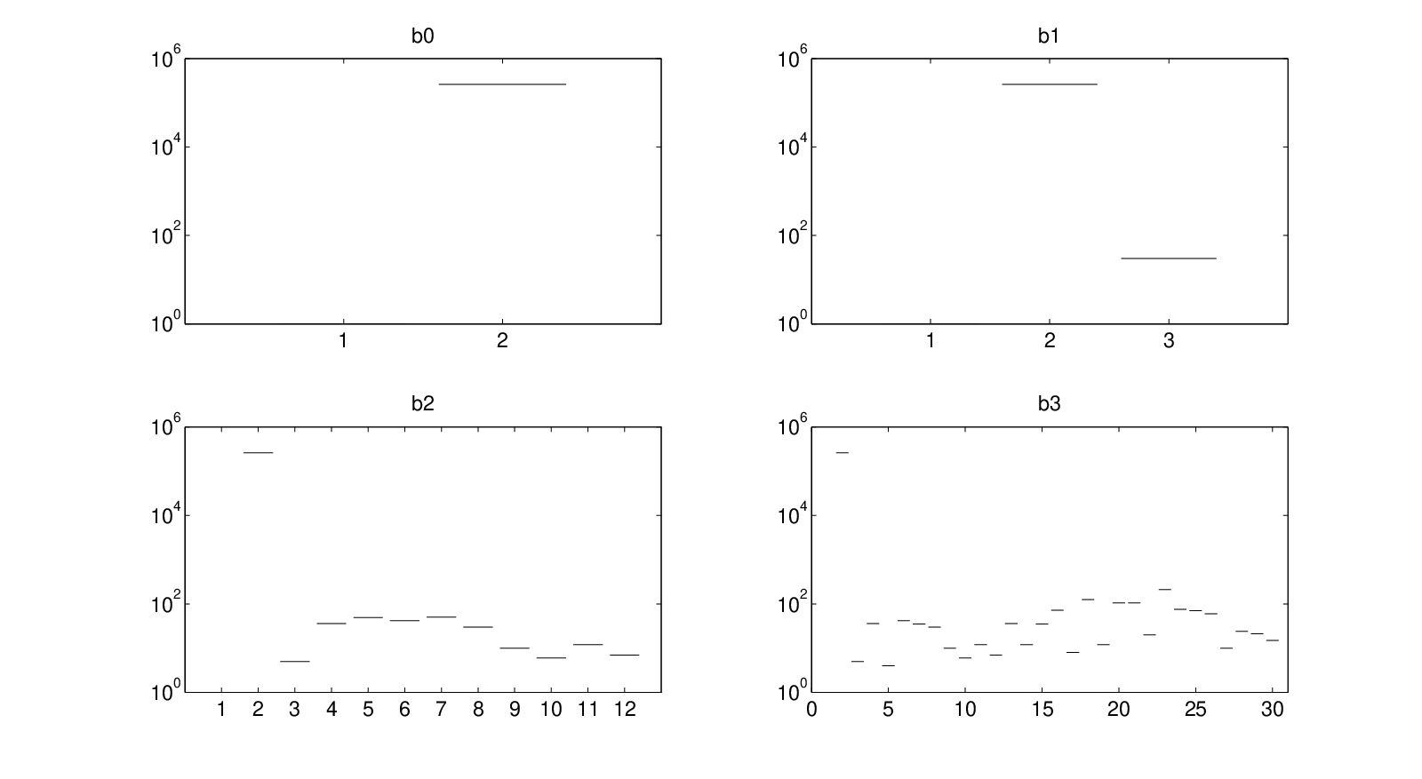
We have tested two target algorithms on a coupon collector problem with $n=18$ objects. In this case $P$ is given by a $2^{18}\times 2^{18}$ -sparse matrix. The computation of $P^{n}$ is not practicable. The number of components of each class of $X/\pi_{m}$ is plotted for $m=0,1,2,3$ in the following Figure 1 and Figure 2. The sequence $(X/\pi_{m})_{m}$ varies according to the target algorithm. We remark that both strategies converge to the same exact solution.

Refer to caption — Fig 1: Number of states for each class of $X/\pi_{m}$ (log scale), with $\epsilon_{1}=0.5$ , $\epsilon_{2}=0.1$ , $\epsilon_{3}=0.05$ . The choice of $(\sim_{\epsilon_{n}})_{n}$ is made as in Example 2.

4 Blackwell

The problem of approximation is mathematically different if we start from a Markov process with a countable set of states or with an uncountable one. Let us consider, for the moment, the countable case: $X$ is the at most countable set of the states and $\mathcal{X}=2^{X}$ is the power set. Each function on $X$ is measurable. If we take any equivalence relation on $X$ , it is both measurable and identified by the $\sigma$ -algebra it induces (see Theorem 11 below). This is not in general the case when we deal with a measurable space $(X,\mathcal{X})$ , with $X$ uncountable. In this section, we want to connect the process of approximation with the upgrading information. More precisely, a measurable equivalence $\pi=\pi_{f}$ defines both the partition $X/\pi$ and the sigma algebra $\sigma(f)$ . One wishes these two objects to be related, in the sense that ordering should be preserved. Example 7 below shows a paradox concerning $\pi_{f}$ and $\sigma(f)$ when $X$ is uncountable. In fact,

Lemma 9.

Let $\mathcal{A}_{1}\subseteq\mathcal{A}_{2}$ be countably generated sub $\sigma$ -algebras of a measurable space $(X,\mathcal{X})$ . Then $[x]_{\mathcal{A}_{1}}\supseteq[x]_{\mathcal{A}_{2}}$ .

In particular, let $f,g$ be random variables. If $\sigma(f)\supseteq\sigma(g)$ , then $\pi_{f}\subseteq\pi_{g}$ .

See Appendix A. ∎The problem is that even if a partition is more informative than another one, it is not true that it generates a finer $\sigma$ -algebra, i.e., the following implication is not always true for any couple of random variables $f$ and $g$

\pi_{f}\subseteq\pi_{g}\Longrightarrow\sigma(f)\supseteq\sigma(g).

(A0)

Then Lemma 9 is not invertible, if we do not require the further Assumption (A0) on the measurable space $(X,\mathcal{X})$ . This last fact connects the space $(X,\mathcal{X})$ with the theory of Blackwell spaces (see Lemma 10). We will assume the sole Assumption (A0).

Example 5 ( $\pi_{f}=\pi_{g}\nRightarrow\sigma(f)=\sigma(g)$ ).

We give here a counterexample to Assumption (A0), where two random variables $f,g$ generate two different sigma algebras $\sigma(f)\neq\sigma(g)$ with the same set of atoms. Obviously, Assumption (A0) does not hold.

Let $(X,{\mathcal{B}}_{X})$ be a Polish space and suppose ${\mathcal{B}}_{X}\subsetneq\mathcal{X}$ . Let $A\in\mathcal{X}\setminus{\mathcal{B}}_{X}$ and consider the sequence $\{A_{n},n\in\mathbb{N}\}$ that determines ${\mathcal{B}}_{X}$ , i.e. ${\mathcal{B}}_{X}=\sigma(A_{n},n\in\mathbb{N})$ . Let $\mathcal{A}=\sigma(A,A_{n},n\in\mathbb{N})$ . ${\mathcal{B}}_{X}\subsetneq\mathcal{A}$ . As a consequence of Lemma A.3, there exist two random variables $f,g$ such that ${\mathcal{B}}_{X}=\sigma(f)$ and $\mathcal{A}=\sigma(g)$ . The atoms of ${\mathcal{B}}_{X}$ are the points of $X$ , and then the atoms of ${\mathcal{A}}$ are also the points of $X$ , since ${\mathcal{B}}_{X}\subseteq\mathcal{A}$ .

We recall here the definition of Blackwell spaces. A measurable space $(X,\mathcal{X})$ is said Blackwell if $\mathcal{X}$ is a countably generated $\sigma$ -algebra of $X$ and $\mathcal{A}=\mathcal{X}$ whenever $\mathcal{A}$ is another countably generated $\sigma$ -algebra of $X$ such that $\mathcal{A}\subseteq\mathcal{X}$ , and $\mathcal{A}$ has the same atoms as $\mathcal{X}$ . A metric space $X$ is Blackwell if, when endowed with its Borel $\sigma$ -algebra, it is Blackwell. The measurable space $(X,\mathcal{X})$ is said to be a strongly Blackwell space if $\mathcal{X}$ is a countably generated $\sigma$ -algebra of $X$ and

(A1)

$\mathcal{A}_{1}=\mathcal{A}_{2}$ if and only if the sets of their atoms coincide, where $\mathcal{A}_{1}$ and $\mathcal{A}_{2}$ are countably generated $\sigma$ -algebras with $\mathcal{A}_{i}\subseteq\mathcal{X}$ $i=1,2$ .

For what concerns Blackwell spaces, the literature is quite extensive. D. Blackwell proved that every analytic subset of a Polish space is, with respect to its relative Borel $\sigma$ -field, a strongly Blackwell space (see [5]). Therefore, if $(X,\mathcal{B}_{X})$ is (an analytic subset of) a Polish space and $\mathcal{B}_{X}\subsetneq\mathcal{X}$ , then $(X,\mathcal{X})$ cannot be a weakly Blackwell space. To see this, take $A_{1},A_{2}\ldots$ a base of $\mathcal{B}_{X}$ and $A\in\mathcal{X}\setminus\mathcal{B}_{X}$ . Then $\mathcal{B}_{X}=\sigma(A_{1},A_{2}\ldots)$ and $\mathcal{A}=\sigma(A,A_{1},A_{2}\ldots)$ have the same set of atoms (the points of $X$ ) but ${\mathcal{A}}\nsubseteq{\mathcal{B}}_{X}$ (or, equivalently, the identity function $I_{d}:(X,\mathcal{B}_{X})\to(X,\mathcal{A})$ is not measurable). Moreover, as any (at most) countable set equipped with any $\sigma$ -algebra may be seen as an analytic subset of a Polish space, then it is a strongly Blackwell space.

A. Maitra exhibited coanalytic sets that are not Blackwell spaces (see [10]). M. Orkin constructed a nonanalytic (in fact nonmeasurable) set in a Polish space that is a Blackwell space (see [11]). Jasiński showed (see [7]) that continuum hypothesis (CH) implies that there exist uncountable Sierpiński and Luzin subsets of $\mathbb{R}$ which are Blackwell spaces (implying in a strong way that Blackwell spaces do not have to be Lebesgue measurable or have the Baire property). Jasiński also showed that CH implies that there exist uncountable Sierpiński and Luzin subsets of $\mathbb{R}$ which are not Blackwell spaces (implying in a strong way that Lebesgue measurable sets and sets with the Baire property do not have to be Blackwell spaces). This latter result is strengthened by R.M. Shortt in [13] by showing that CH implies the existence of uncountable Sierpiński and Luzin subsets of $\mathbb{R}$ which are highly non-Blackwell in the sense that all Blackwell subspaces of the two sets are countable.

Note that Assumption (A0) and Assumption (A1) coincide, as the following Lemma states.

Lemma 10.

Let $(X,\mathcal{X})$ be a measurable space. Then (A0) holds if and only if (A1) holds.

Lemma A.3 in appendix states that $\mathcal{A}\subseteq\mathcal{X}$ is countably generated if and only if there exists a random variable $f$ such that $\mathcal{A}=\sigma(f)$ . In addition, as a consequence of Lemma 9, we have only to prove that (A1) implies (A0). By contradiction, assume (A1), $\pi_{f}\subseteq\pi_{g}$ , but $\sigma(g)\nsubseteq\sigma(f)$ . We have $\sigma(f,g)\neq\sigma(f)$ , and then $\pi_{\sigma(f,g)}\neq\pi_{f}$ by (A1) and Lemma A.3. On the other hand, as a consequence of Eq. (3), we have that $\pi_{\sigma(f,g)}=\pi_{\sigma(f)\vee\sigma(g)}=\pi_{f}\cap\pi_{g}=\pi_{f}$ . ∎We call weakly Blackwell space a measurable space $(X,\mathcal{X})$ such that Assumption (A0) holds. If $(X,\mathcal{X})$ is a weakly Blackwell space, then $(X,\mathcal{F})$ is a weakly Blackwell space, for any $\mathcal{F}\subseteq\mathcal{X}$ . Moreover, every strong Blackwell space is both a Blackwell space and a weakly Blackwell space whilst the other inclusions are not generally true. In [8, 12], examples are provided of Blackwell spaces which may be shown not to be weakly Blackwell. The following example shows that a weakly Blackwell space need not be Blackwell.

Example 6 (weakly Blackwell $\nRightarrow$ Blackwell).

Let $X$ be an uncountable set and $\mathcal{X}$ be the countable–cocountable $\sigma$ -algebra on $X$ . $\mathcal{X}$ is easily shown to be not countably generated, and therefore $(X,\mathcal{X})$ is not a Blackwell space. Take any countably generated $\sigma$ -field $\mathcal{A}\subseteq\mathcal{X}$ , i.e. $\mathcal{A}=\sigma(\{A_{i},i\in\mathbb{N}\})$ .

•

Since each set (or its complementary) of $\mathcal{X}$ is countable, then, without loss of generality, we can assume the cardinality of $X\setminus A_{i}$ to be countable.
•

Each atom $B$ of $\sigma(A_{i},i\in\mathbb{N})$ is of the form

$B=\cap_{i=1,2,\ldots}C_{i},\qquad\text{where $C_{i}=A_{i}$ or $C_{i}=X\setminus A_{i}$, for any $i$.}$ (8)

Note that the cardinality of the set $A:=\cup_{i}(X\setminus A_{i})$ is countable, as it is a countable union of countable sets. As a consequence of (8), we face two types of atoms:

1.

for any $i$ , $C_{i}=A_{i}$ . This is the atom made by the intersections of all the uncountable generators. This is an uncountable atom, as it is equal to $X\setminus A$ .
2.

exists $i$ such that $C_{i}=X\setminus A_{i}$ . This implies that this atom is a subset of the countable set $A$ . Therefore, all the atoms (except $X\setminus A$ ) are disjoint subsets of the countable set $A$ and hence they are countable.

It follows that the number of atoms of $\mathcal{A}$ is at most countable. Thus, $(X,\mathcal{A})$ is a strongly Blackwell space, i.e. $(X,\mathcal{X})$ is a weakly Blackwell space.

Example 7 (Information and $\sigma$ -algebra (see [6])).

Suppose $X=[0,1]$ , $\mathcal{X}=\sigma(\mathcal{Y},A)$ where $\mathcal{Y}$ is the countable–cocountable $\sigma$ -algebra on $X$ and $A=[0,1/2)$ . Consider a decisionmaker who chooses action 1 if $x<\frac{1}{2}$ and action 2 if $x\geq\frac{1}{2}$ . Suppose now that the information is modeled either as the partition of all elements of $X$ , $\tau=\{x,x\in X\}$ and in this case the decisionmaker is perfectly informed, or as the partition $\tau^{\prime}=\{A,X\setminus A\}.$ If we deal with $\sigma$ -algebras as a model of information then $\sigma(\tau)=\mathcal{Y}$ and $\sigma(\tau^{\prime})=\sigma(A)$ . The partition $\tau$ is more informative than $\tau^{\prime}$ , whereas $\sigma(\tau)$ is not finer than $\sigma(\tau^{\prime})$ . In fact $A\not\in\mathcal{Y}$ and therefore if the decisionmaker uses $\sigma(\tau)$ as its structure of information, believing it more detailed than $\sigma(\tau^{\prime})$ , he will never know whether or not the event $A$ has occurred and can be led to take the wrong decision. In this case, $\sigma$ -algebras do not preserve information because they are not closed under arbitrary unions. However, if we deal with Blackwell spaces, any countable $\sigma$ -algebra is identified by its atoms and therefore will possess an informational content (see [14], for example).

The following theorem, whose proof is in Appendix B, links the measurability of any relation with the cardinality of the space and Assumption (A0). It shows the main difference between the uncountable case and the countable one.

Theorem 11.

Assume (CH). Let $(X,\mathcal{X})$ be a measurable space. The following properties are equivalent:

1.

Any equivalence relation $\pi$ on $X$ is measurable and Assumption (A0) holds;
2.

$(X,2^{X})$ is a weakly Blackwell space;
3.

$X$ is countable and $\mathcal{X}=2^{X}$ .

5 Proofs

The following theorem mathematically motivates our approximation problem: any limit of a monotone sequence of discrete equivalence relationships is a measurable equivalence.

Theorem 12.

For all $n\in\mathbb{N}$ , let $\pi_{n}$ be a discrete equivalency. Then $\pi_{\infty}=\cap_{n}\pi_{n}$ is a measurable equivalency. Conversely, for any measurable equivalency $\pi$ , there exists a sequence $(\pi_{n})_{n}$ of discrete equivalencies such that $\pi_{\infty}=\cap_{n}\pi_{n}$ .

See Appendix A. ∎

Let $\pi=\pi_{f}$ be a compatible projection. We define

P_{\pi}(x,F):=P(x,F),\qquad\forall x\in X,\forall F\in\sigma(f).

What remains to prove is that $P_{\pi}\in\mathrm{TrP}(X,\mathcal{X},\sigma(f))$ . More precisely, we have to show that $P_{\pi}(\cdot,F)$ is $\sigma(f)$ -measurable, $\forall F\in\sigma(f)$ . By contradiction, there exists $F\in\sigma(f)$ such that the random variable $Y^{F}(\omega)=P_{\pi}(\omega,F)$ is not $\sigma(f)$ -measurable. Then $\sigma(Y^{F})\nsubseteq\sigma(f)$ , and hence $\pi_{Y^{F}}\nsupseteq\pi_{f}$ by Assumption (A0), which contradicts Equation (1). ∎

As a consequence of Theorem 12, $\pi_{\infty}=\pi_{f}$ , where $\sigma(f)=\vee_{n}\mathcal{F}_{n}$ . Define

P_{\infty}(x,F):=P(x,F),\qquad\forall x\in X,\forall F\in\sigma(f).

We will prove that, for any $F\in\sigma(f)$ , $P_{\infty}(\cdot,F)$ is $\sigma(f)$ -measurable and consequently $\pi_{\infty}$ will be a compatible projection. This implies that there exists a measurable function $h_{F}:(\mathbb{R},\mathcal{B}_{R})\to(\mathbb{R},\mathcal{B}_{R})$ so that $P_{\infty}(\omega,F)=h_{F}(f(\omega))$ . Therefore, if $x\,\pi_{f}\,y$ , then $P_{\infty}(x,F)=P_{\infty}(y,F)$ , which is the thesis.

Thus, we show that for any $F\in\sigma(f)$ and $t\in\mathbb{R}$ , we have

H:=\{x\colon P(x,F)\leq t\}\in\sigma(f)

(9)

To prove Equation (9), we first show that it is true when $F\in\mathcal{F}_{n}$ by proving that

H=\cap_{m>n}\pi^{-1}_{m}\pi_{m}(H),

which implies that $H\in\sigma(f)$ . The inclusion $H\subseteq\cap_{m}\pi^{-1}_{m}\pi_{m}(H)$ is always true. For the other inclusion, let $y\in\cap_{m>n}\pi^{-1}_{m}\pi_{m}(H)$ . Let $m>n$ ; there exists $x_{m}\in H$ such that $y\pi_{m}x_{m}$ . Therefore, Equation (4) and the definition of $\sim_{\epsilon_{n}}$ imply $P(y,F)\leq P(x_{m},F)+\epsilon_{m}\leq t+\epsilon_{m}$ , for any $m>n$ . As $\epsilon_{m}\searrow 0$ , we obtain that $y\in H$ . Then Equation (9) is true on the algebra $Alg:=\cup_{n}\mathcal{F}_{n}$ .

Actually, let $F_{n}\in Alg$ such that $F_{n}\nearrow F$ . We prove that Equation (9) holds for $F$ by showing that

H=\{x\colon P(x,F)\leq t\}=\cap_{n}\{x\colon P(x,F_{n})\leq t\}=:\cap_{n}H_{n}.

Again, since $F_{n}\subseteq F$ , then $P(x,F_{n})\leq P(x,F)$ and therefore $H\subseteq\cap_{n}H_{n}$ . Conversely, the set $\cap_{n}H_{n}\setminus H$ is empty since the sequence of $\mathcal{X}$ -measurable maps $P(\cdot,F)-P(\cdot,F_{n})$ converges to $0$ :

P(\cdot,F)-P(\cdot,F_{n})=P(\cdot,F\setminus F_{n})\to P(\cdot,\varnothing)=0.

Then Equation (9) is true on the monotone class generated by the algebra $Alg=\cup_{n}\mathcal{F}_{n}$ , i.e., Equation (9) is true on $\sigma(f)$ . ∎

Given a target algorithm $(X,\mathcal{F}_{n},T,P_{n})_{n}$ , let $\pi_{\infty}=\pi_{f}$ be defined as in Theorem 8. We show that $\pi_{\infty}$ is optimal. Let $\psi_{g}$ be another compatible projection and let $(X,\sigma(g),T,P_{g})$ be the target problem given by Theorem 2. We are going to prove by induction on $n$ that

\forall n\in\mathbb{N},\qquad\mathcal{F}_{n}\subseteq\sigma(g).

(10)

In fact, for $n=0$ it is sufficient to note that $\mathcal{F}_{0}=\sigma(\{T\})\subseteq\sigma(g)$ .

Equation (4) states that $\mathcal{F}_{n}=\sigma(\mathcal{F}_{n-1},h_{n})$ , where $h_{n}$ is the discrete random variable, given by Lemma 6, s.t.

	$\displaystyle x\,$	$\displaystyle\pi_{h_{n}}\,y$
		$\displaystyle\Updownarrow$
	$\displaystyle\Big(\big(P(x,A^{(n-1)}_{i})_{i}\big)$	$\displaystyle\sim_{\epsilon_{n}}\big(P(y,A^{(n-1)}_{i})_{i}\big)\Big)$

Let $k^{(n-1)}_{i}:X\to[0,1]$ be defined as $k^{(n-1)}_{i}(x)=P(x,A^{(n-1)}_{i})$ . Then

\begin{diagram}

Obviously, $\sigma(h_{n})\subseteq\sigma(k^{(n-1)}_{1},k^{(n-1)}_{2},\ldots)$ . For the induction step, as $A^{(n-1)}_{i}\in\mathcal{F}_{n-1}\subseteq\sigma(g)$ , we have that $P_{g}(\cdot,A^{(n-1)}_{i})$ is $\sigma(g)$ -measurable, and therefore $\sigma(k^{(n-1)}_{i})\subseteq\sigma(g)$ . Then $\mathcal{F}_{n}=\sigma(\mathcal{F}_{n-1},h_{n})\subseteq\sigma(\mathcal{F}_{n-1},k^{(n-1)}_{1},k^{(n-1)}_{2},\ldots)\subseteq\sigma(g)$ . Therefore $\sigma(f)=\vee_{n}\mathcal{F}_{n}\subseteq\sigma(g)$ , which implies $\pi_{\infty}\supseteq\psi_{g}$ by Lemma 9, and hence $\pi_{\infty}$ is optimal. ∎

Corollary 13.

$\pi_{\infty}$ does not depend on the choice of $\mathrm{Str}$ .

$\pi_{\infty}=\cap_{n}\pi_{n}$ is optimal, $\forall(\pi_{n})_{n}=\mathrm{Str}(P)$ . The optimal projection being unique, we are done. ∎

Let $\pi_{\infty}=\pi_{f}$ be defined as in Theorem 8 and $(X,\sigma(f),T,P_{\infty})$ be given by Theorem 2 so that $P(x,F)=P_{\infty}(x,F)$ for any $F\in\sigma(f)$ . Then each $(P_{n})_{n}$ of Definition 5 can be rewritten as

{P}_{n}(x,F)=\frac{\int_{[x]_{n}}P_{\infty}(x,F)\mu(dz)}{\mu([x]_{n})},\qquad\forall x\in X,\forall F\in{\mathcal{F}}_{n},

(11)

where $[x]_{n}$ is the $\pi_{n}$ -class of equivalence of $x$ and $\mu([x]_{n})>0$ since $[x]_{n}\neq\varnothing$ .

Note that $d(P,{P}_{m})\leq 2\sum_{n}\beta^{n}$ . Then, for any $\epsilon>0$ , there exists an $N$ so that $\sum_{n>N}\beta^{n}\leq\frac{\epsilon}{2}$ . Therefore we are going to prove by induction on $n$ that

\sup_{x}|{P}^{n}_{m}(x,T)-P^{n}(x,T)|\rightarrow 0\text{ as }m\text{ tends to infinity},

which completes the proof. If $n=1$ , then by definition of $\epsilon_{m}$ , since $T\in{\mathcal{F}}_{m-1}$ , we have that

	$\displaystyle\|{P}_{m}(x,T)-P(x,T)\|$	$\displaystyle\leq\frac{\int_{[x]_{n}}\|P_{\infty}(z,T)-P(x,T)\|\mu(dz)}{\mu([x]_{n})}$
		$\displaystyle=\frac{\int_{[x]_{n}}\|P(z,T)-P(x,T)\|\mu(dz)}{\mu([x]_{n})}$
		$\displaystyle\leq\epsilon_{m}\frac{\int_{[x]_{n}}{\mu(dz)}}{\mu([x]_{n})}=\epsilon_{m}.$

For the induction step, we note that

\big|{P}^{n+1}_{m}(x,T)-P^{n+1}(x,T)\big|\\ \leq\sum_{i}\Big|{P}_{m}(x,A_{i}^{(m)}){P}^{n}_{m}(A_{i}^{(m)},T)-\int_{A_{i}^{(m)}}P(x,dz)P^{n}(z,T)\Big|,

(12)

where $(A_{i}^{(m)})_{i}$ is the partition of $X$ given by $\pi_{m}$ . By induction hypothesis,

|{P}^{n}_{m}(z,T)-P^{n}(z,T)|\leq\epsilon

for $m\geq m_{0}$ large enough. Since $[z]_{m}=A_{i}^{(m)}$ if $z\in A_{i}^{(m)}$ , it follows that

\int_{A_{i}^{(m)}}P(x,dz)\Big|{P}^{n}_{m}(A_{i}^{(m)},T)-P^{n}(z,T)\Big|\leq\epsilon\int_{A_{i}^{(m)}}P(x,dz).

Equation (12) becomes

\big|{P}^{n+1}_{m}(x,T)-P^{n+1}(x,T)\big|\\ \leq\epsilon+\sum_{i}{P}^{n}_{m}(A_{i}^{(m)},T)\big|{P}_{m}(x,A_{i}^{(m)})-P(x,A_{i}^{(m)})\big|\\ \leq\epsilon+\sum_{i}\big|{P}_{m}(x,A_{i}^{(m)})-P(x,A_{i}^{(m)})\big|.

On the other hand, by Equation (11),

{P}_{m}(x,A_{i}^{(m)})-P(x,A_{i}^{(m)})=\int_{[x]_{m}}\frac{P_{\infty}(z,A^{(m)}_{i})-P(x,A^{(m)}_{i})}{\mu([x]_{m})}\mu(dz).

The definition of $\sim_{\epsilon_{m+1}}$ states that

\sum_{i}\big|P_{\infty}(z,A^{(m)}_{i})-P(x,A^{(m)}_{i})\big|\leq\epsilon_{m+1}

whenever $z\in[x]_{m}$ and therefore

\big|{P}^{n+1}_{m}(x,T)-P^{n+1}(x,T)\big|\\ \leq\epsilon+\int_{[x]_{m}}\sum_{i}\big|P_{\infty}(z,A^{(m)}_{i})-P(x,A^{(m)}_{i})\big|\frac{\mu(dz)}{\mu([x]_{m})}\leq\epsilon+\epsilon_{m+1}.

Since $\epsilon_{m}\rightarrow 0$ as $m$ tends to infinity, we get the result. ∎

By Definition 5 and Lemma 7, $(P_{n}(\cdot,F))_{n\geq m}$ is a martingale with respect to the filtration $(\mathcal{F}_{n})_{n\geq m}$ , for any $F\in\mathcal{F}_{m}$ . Then, if $Y^{F}(x)=P(x,F)$ as in Definition 5, we have that

P_{n}(x,F)\mathop{\longrightarrow}_{n\to\infty}\mathbb{E}_{\mu}[Y^{F}|\vee_{n}{\mathcal{F}}_{n}](x)=Y^{F}(x),\qquad\text{for $\mu$-a.e. }x\in X,\forall F\in\cup_{m}{\mathcal{F}}_{m}.

Let $\pi_{\infty}=\pi_{f}$ be defined as in Theorem 8 and $(X,\sigma(f),T,P_{\infty})$ given by Theorem 2 so that $P(x,F)=P_{\infty}(x,F)$ for any $F\in\sigma(f)$ . Then

P_{n}(x,F)\mathop{\longrightarrow}_{n\to\infty}P_{\infty}(x,F)

for any $x\in X$ and $F\in\cup_{m}{\mathcal{F}}_{m}$ , the only $\mu$ -null set in $\cup_{m}{\mathcal{F}}_{m}$ being the empty set. ∎

5.1 Weak convergence of conditional probabilities

Let the target problem $(X,\mathcal{F},T,P)$ be given and let $\mathrm{Str}=(\mathrm{Str}_{n})_{n}$ , where $\mathrm{Str}_{n}(X,\mathcal{F},T,P)=(X,\tilde{\mathcal{F}}_{n},T,\tilde{P}_{n})$ be a target algorithm. In order to prove Theorem 5, which states the total convergence of the probability measure ${P}_{n}(x,\cdot)$ towards $P(x,\cdot)$ , we proceed as follows:

•

first, we define the topology $\varrho_{P}$ on $X$ ;
•

then, we define a “natural” topology $\tau_{\mathrm{Str}}$ on $X$ associated to any target algorithm $({\mathrm{Str}_{n}})_{n}$ . We prove in Theorem 14 the total convergence of $(P_{n})_{n}$ to $P_{\infty}$ , under this topology;
•

then, we define the topology $\tau_{P}$ on $X$ as the intersection of all the topologies $\tau_{\mathrm{Str}}$ ;
•

finally, we show Theorem 5 by proving that $\varrho_{P}\subseteq\tau_{\mathrm{Str}}$ . The non-triviality of $\varrho_{P}$ will imply that of $\tau_{P}$ .

We introduce the pseudometric $d_{P}$ on $X$ as follows:

d_{P}(x,y)=\sum_{n}\beta^{n}\big|P^{n}(x,T)-P^{n}(y,T)\big|.

Now, let $\tau_{\mathrm{Str}}$ be the topology generated by $\cup_{n}{\mathcal{F}}_{n}$ . $C$ is a closed set if and only if $C=\cap_{n}C_{n},C_{n}\in{{\mathcal{F}}_{n}}$ . In fact, if $C\in{\mathcal{F}}_{n}$ , for a given $n$ , then $C\in{\mathcal{F}}_{n+p}$ , for any $p$ and therefore $C$ is closed. $(X,\tau_{\mathrm{Str}})$ is a topological space.

Remark 5.

Let us go back to Example 1. The topology defined by asking that the sets in each $\mathcal{F}_{n}$ are closed is strictly finer than the standard topology. On the other hand, the same example may be explained with left closed–right opened dyadic subdivisions, which leads to a different topology that also contains the natural one. Any other “reasonable” choice of subdivision will show the same: the topologies are different, and all contain the standard one. In the same manner, we are going to show that all the topologies $\tau_{\mathrm{Str}}$ contain the standard one, $\varrho_{P}$ .

Theorem 14.

Let the target problem $(X,\mathcal{F},T,P)$ and the target algorithm $(X,\mathcal{F}_{n},T,P_{n})_{n}$ be given. For any target algorithm $\mathrm{Str}$ ,

{P}_{n}(x,\cdot)\mathop{\longrightarrow}\limits^{\mathrm{tot}}_{\tau_{\mathrm{Str}}}P(x,\cdot),\qquad\forall x\in X.

Let $C=\cap_{n}C_{n}$ be a closed set of $\mathrm{Str}$ and let $\bar{P}_{n}$ be any extension of ${P}_{n}$ to $\vee_{n}\mathcal{F}_{n}$ . We have to check that ${\limsup}_{n}\bar{P}_{n}(x,C)\leq P(x,C)$ , for any given $x$ (see, e.g., [4]). Note that, since $C\in\vee_{n}\mathcal{F}_{n}$ , we have $P(x,C)=P_{\infty}(x,C)$ . But, $\bar{P}_{n}(x,C)-P_{\infty}(x,C)\leq\bar{P}_{n}(x,C_{n-1})-P_{\infty}(x,C)={P}_{n}(x,C_{n-1})-P_{\infty}(x,C)$ . Actually,

{P}_{n}(x,C_{n-1})-P_{\infty}(x,C)\\ =\Big(\underbrace{{P}_{n}(x,C_{n-1})-P_{\infty}(x,C_{n-1})}_{I}\Big)+\Big(\underbrace{P_{\infty}(x,C_{n-1})-P_{\infty}(x,C)}_{II}\Big).

$I\rightarrow 0$ as $n$ tends to infinity, from the target algorithm, since as $\epsilon_{n}\searrow 0$ . For any $\epsilon>0$ , there exists $N_{1}>0$ , such that for any $n\geq N_{1}$ , $|{P}_{n}(x,C_{n-1})-P_{\infty}(x,C_{n-1})|\leq\frac{\epsilon}{2}$ .
$II\rightarrow 0$ as $n$ tends to infinity, from the continuity of the measure. For any $\epsilon>0$ , there exists $N_{2}>0$ and for any $n\geq N_{2}$ , $|P_{\infty}(x,C_{n-1})-P_{\infty}(x,C)|\leq\frac{\epsilon}{2}.$ ∎

An example of a natural extension of $P_{n}$ to $\bar{P}_{n}$ is given by

\bar{P}_{n}(x,F)=\mathbb{E}_{\mu}[Y^{F}|\vee_{n}\mathcal{F}_{n}](x),\qquad\forall x\in X,\forall F\in\vee_{n}\mathcal{F}_{n},

where, for any $F\in\vee_{n}\mathcal{F}_{n}$ , $Y^{F}$ is the $\vee_{n}{\mathcal{F}}_{n}$ -random variable such that $Y^{F}(\omega)=P_{\infty}(\omega,F)$ . As mentioned for ${P}_{n}$ , $\bar{P}_{n}(x,\cdot)$ is a probability measure, for any $x\in X$ .

Corollary 15.

For any fixed strategy $\mathrm{Str}(P)$ , let $P_{n}$ be as in Theorem 1. We have

{P}_{n}(x,\cdot)\mathop{\longrightarrow}\limits^{\mathrm{tot}}_{\tau_{P}}P(x,\cdot),

for any given $x$ .

In order to describe the topology $\tau_{P}$ , we will denote by $[[F]]_{*}$ the closure of a set $F\subseteq X$ in a given topology $*$ . Note that the monotonicity of $\pi_{n}$ implies

[[F]]_{\tau_{\mathrm{Str}}}=\cap_{n}[[F]]_{\tau_{\mathrm{Str}_{n}}}

where $\tau_{\mathrm{Str}_{n}}$ is the (discrete) topology on $X$ generated by $\mathcal{F}_{n}$ . Since $\tau_{P}$ is the intersection of all the topologies $\tau_{\mathrm{Str}}$ , we have

[[F]]_{\tau_{P}}\supseteq[[F]]_{\tau_{\mathrm{Str}}}=\cap_{n}[[F]]_{\tau_{\mathrm{Str}_{n}}},\qquad\forall F\in 2^{X},\forall\mathrm{Str}.

Let $F$ be the closed set in $\varrho_{P}$ so defined

F:=\{y\in X\colon d_{P}(y,x)\geq r\},

i.e., $F$ is the complementary of an open ball in $(X,d_{P})$ with center $x$ and radius $r$ . If we show that $F\in\tau_{P}$ , then we are done, since the arbitrary choice of $x$ and $r$ spans a base for the topology $\varrho_{P}$ .

We are going to prove

F=[[F]]_{\tau_{\mathrm{Str}}}=\cap_{m}[[F]]_{\tau_{\mathrm{Str}_{m}}},\qquad\forall\mathrm{Str},

which implies $[[F]]_{\tau_{P}}=F$ . It is always true that $F\subseteq[[F]]_{*}$ ; we prove the nontrivial inclusion $F\supseteq\cap_{m}[[F]]_{\tau_{\mathrm{Str}_{m}}}$ . Assume that $y\in[[F]]_{\tau_{\mathrm{Str}}}$ . Now, $y\in[[F]]_{\tau_{\mathrm{Str}_{m}}}$ , for any $m$ , and then there exists a sequence $(y_{m})_{m}$ with $y_{m}\in F$ such that $y\,\pi_{m}\,y_{m}$ , for any $m$ . Thus, $y\in\cap_{m}[y_{m}]_{m}$ , where $[x]_{m}$ is the $\pi_{m}$ -class of equivalence of $x$ . Thus

P^{n}_{m}(y_{m},T)=P^{n}_{m}(y,T),\qquad\forall m,n

since $P_{m}(\cdot,T)$ is $\mathcal{F}_{m}$ -measurable. By Theorem 1, for any $n\in\mathbb{N}$ ,

|P^{n}(y,T)-P_{m}^{n}(y,T)|+|P_{m}^{n}(y_{m},T)-P^{n}(y_{m},T)|\mathop{\longrightarrow}_{m\to\infty}0.

Now, let $N$ be such that $\sum_{n=N}^{\infty}\beta^{n}\leq\frac{\epsilon}{4}$ and take $n_{0}$ sufficiently large s.t.

\sum_{n=0}^{N}|P^{n}(y,T)-P_{n_{0}}^{n}(y,T)|+|P_{n_{0}}^{n}(y_{n_{0}},T)-P^{n}(y_{n_{0}},T)|\leq\frac{\epsilon}{2}

We have

d_{P}(y_{n_{0}},y)=\sum_{n}\beta^{n}\big|P^{n}(y,T)-P^{n}(y_{n_{0}},T)\big|\ \\ \leq\sum_{n=0}^{N}\big|P^{n}(y,T)-P^{n}(y_{n_{0}},T)\big|\ +2\sum_{n=N}^{\infty}\beta^{n}\\ \leq\sum_{n=0}^{N}\Big(|P^{n}(y,T)-P_{n_{0}}^{n}(y,T)|+|P^{n}_{n_{0}}(y,T)-P^{n}_{n_{0}}(y_{n_{0}},T)|\\ +|P_{n_{0}}^{n}(y_{n_{0}},T)-P^{n}(y_{n_{0}},T)|\Big)+2\frac{\epsilon}{4}\leq\frac{\epsilon}{2}+\frac{\epsilon}{2}=\epsilon.

and therefore

d_{P}(x,y)\geq d_{P}(x,y_{n_{0}})-d_{P}(y_{n_{0}},y)\geq r-\epsilon.

The arbitrary choice of $\epsilon$ implies $y\in F$ , which is the thesis. ∎

A Results on equivalence relations

In this appendix we give the proof of auxiliary results that connect equivalency with measurability.

Let $\pi=\pi_{f}$ be a discrete equivalency on $X$ . Then $X/\pi$ defines a countable measurable partition of $X$ . Conversely, let $\{A_{1},A_{2},\ldots\}$ be a countable measurable partition on $X$ . Define $f:X\to\mathbb{N}$ s.t. $f(x)=n\iff x\in A_{n}$ . Therefore $f$ is measurable and $\pi=\pi_{f}$ is a discrete equivalency on $X$ . ∎

Lemma A.1.

Let $f,g$ be two random variables such that $g(x)<g(y)\Rightarrow f(x)<f(y)$ . Then $\sigma(g)\subseteq\sigma(f)$ .

Let $t\in\mathbb{R}$ be fixed. We must prove that $\{g\leq t\}\in\sigma(f)$ . If $\{g\leq t\}=$ or $\{g>t\}$ are empty, then we are done. Assume then that $\{g\leq t\},\{g>t\}\neq\varnothing$ . We have two cases

- ${t^{\ast}\in f(\{g\leq t\})}$ : $\exists x^{\ast}\in\{g\leq t\}$ such that $t^{\ast}=f(x^{\ast})$ .
By definition of $t^{\ast}$ , $\{g\leq t\}\subseteq\{f\leq t^{*}\}$ . Conversely, let $y\in\{g>t\}$ . Since $g(x^{\ast})\leq t<g(y)$ , then $f(x^{\ast})=t^{\ast}<f(y)$ , i.e. $\{g>t\}\subseteq\{f>t^{*}\}$ . Then $\{g\leq t\}=\{f\leq t^{\ast}\}\in\sigma(f)$ .

- ${t^{\ast}\not\in f(\{g\leq t\})}$ : $\forall x\in\{g\leq t\}$ we have that $f(x)<t^{\ast}$ .
Then $\{g\leq t\}\subseteq\{f<t^{*}\}$ . Conversely, let $y\in\{g>t\}$ . Since $\forall x\in\{g\leq t\}$ $g(y)>g(x)$ , then $f(y)>f(x)$ , which implies $f(y)\geq\sup f(\{g\leq t\})=t^{\ast}$ , i.e. $\{g>t\}\subseteq\{f\geq t^{*}\}$ . Then $\{g\leq t\}=\{f<t^{\ast}\}\in\sigma(f)$ . ∎

The next lemma plays a central rôle. Its proof is common in set theory.

Lemma A.2.

For all $n\in\mathbb{N}$ , let $\pi_{n}$ be a discrete measurable equivalency. Then there exists a random variable $f$ such that $\sigma(f)=\vee_{n}\sigma({X/\pi_{n}})$ .

Before proving the core of the Lemma, we build a sequence $(g_{n})_{n\in\mathbb{N}}$ of functions $g_{n}:\mathbb{N}^{n}\to\mathbb{R}$ that will be used to define the function $f$ .

Take $h:\mathbb{N}\cup\{0\}\to[0,1)$ to be the increasing function $h(m)=1-2^{-m}$ and let $(g_{n})_{n\in\mathbb{N}}$ the sequence of function $g_{n}:\mathbb{N}^{n}\to\mathbb{R}$ so defined:

		$\displaystyle g_{1}(m_{1})=h(m_{1}-1)$
		$\displaystyle g_{2}(m_{1},m_{2})=g_{1}(m_{1})+h(m_{2}-1)\Delta g_{1}(m_{1})$

		$\displaystyle g_{n+1}(\mathbf{m}_{n},m_{n+1})=g_{n}(\mathbf{m}_{n})+h(m_{n+1})\Delta g_{n}(\mathbf{m}_{n})$

where, for all $n$ , $\mathbf{m}_{n}=(m_{1},\ldots,m_{n})$ and

\Delta g_{n}(\mathbf{m}_{n})=g_{n}(\mathbf{m}_{n-1},m_{n}+1)-g_{n}(\mathbf{m}_{n-1},m_{n}).

As a first consequence of the definition, note that for any choice of $n$ and $\mathbf{m}_{n+1}$ , it holds that

g_{n}(\mathbf{m}_{n-1},m_{n})\leq g_{n+1}(\mathbf{m}_{n+1})<g_{n}(\mathbf{m}_{n-1},m_{n}+1)

(13)

since $h\in[0,1)$ . We now prove by induction on $n_{1}+n_{2}$ that for any choice of $n_{1}\in\mathbb{N}$ , $n_{2}\in\mathbb{N}\cup\{0\}$ and $\mathbf{m}_{n_{1}+n_{2}}$ , we have

g_{n_{1}}(\mathbf{m}_{n_{1}-1},m_{n})\leq g_{n_{1}+n_{2}}(\mathbf{m}_{n_{1}+n_{2}})<g_{n_{1}}(\mathbf{m}_{n_{1}-1},m_{n}+1).

(14)

Eq. (14) is clearly true for $n_{1}+n_{2}=1$ , since $h$ is strictly monotone. The same argument shows that Eq. (14) is always true for $n_{2}=0$ and therefore we check it only for $n_{2}>0$ . We assume by induction that Eq. (14) is true for $n_{1}+n_{2}\leq n$ and we prove it for $n_{1}+n_{2}=n+1$ . By using twice the induction hypothesis, as $n_{2}-1\geq 0$ , we obtain

	$\displaystyle g_{n_{1}}(\mathbf{m}_{1},m_{n})$	$\displaystyle\leq g_{n_{1}+n_{2}-1}(\mathbf{m}_{n_{1}+n_{2}-2},m_{n_{1}+n_{2}-1})$
		$\displaystyle<g_{n_{1}+n_{2}-1}(\mathbf{m}_{n_{1}+n_{2}-2},m_{n_{1}+n_{2}-1}+1)$
		$\displaystyle\leq g_{n_{1}}(\mathbf{m}_{1},m_{n}+1).$

Eq. (14) is now a consequence of Eq. (13).

Now, we come back to the proof of the Lemma. First note that, without loss of generality, we can (and we do) require the sequence $(\pi_{n})_{n\in\mathbb{N}}$ to be monotone, by taking the sequence $\pi^{\prime}_{n}=\cap_{i=1}^{n}\pi_{i}$ instead of $\pi_{n}$ . $\pi^{\prime}_{n}$ is again a countable measurable equivalency on $X$ . In fact, by Lemma 6 we can read this statement in trivial terms of partitions: since at most countable intersection of families of countable measurable partition is a countable measurable partition. Moreover, by definition, $\vee_{i=1}1^{n}\sigma(X/\pi_{i})=\vee_{i=1}1^{n}\sigma(X/\pi^{\prime}_{i})$ .

Let $\tau_{n}=X/\pi_{n}$ be the increasing sequence of countable measurable dissections of $X$ . We are going to give a consistent inductive method of numbering the set of atoms of $\tau_{n}$ to build the functions $f_{n}$ . Let $\tau_{1}=\{A_{1}^{(1)},A_{2}^{(1)},\ldots\}$ be any ordering of $\tau_{1}$ . By induction, let $\{A_{\mathbf{m}_{n},1}^{(n+1)},A_{\mathbf{m}_{n},2}^{(n+1)},\ldots\}$ be the partition of the atom $A_{\mathbf{m}_{n}}^{(n)}\in\tau_{n}$ given by $\tau_{n+1}$ . Define, for any $n\in\mathbb{N}$ ,

f_{n}(x)=g_{n}(\mathbf{m}_{n})\qquad\iff\qquad x\in A_{\mathbf{m}_{n}}^{(n)}.

To complete the proof, we first show that $\sigma(f_{n})=\sigma(X/\pi_{n}),\forall n$ , and then we prove $\sigma(f)=\sigma(f_{1},f_{2},\ldots)$ by proving that $f_{n}\to f$ pointwise.

To prove that $\sigma(f_{n})=\sigma(X/\pi_{n})$ we show that $f_{n}(x)=f_{n}(y)\iff\exists\mathbf{m}_{n}\colon x,y\in A_{\mathbf{m}_{n}}^{(n)}$ . One implication is a consequence of the fact that $f_{n}$ is defined on the partition of $X$ given by $X/\pi_{n}=\tau_{n}$ . For the converse, assume that $x\in A_{\mathbf{m}_{n}}^{(n)}\neq A_{\mathbf{m}_{n}^{\prime}}^{(n)}\ni y$ and consider $n_{1}:=\min\{j\leq n\colon m_{j}\neq m_{j}^{\prime}\}$ . Thus $\mathbf{m}_{n_{1}-1}=\mathbf{m}_{n_{1}-1}^{\prime}$ and, without loss of generalities, $m_{n_{1}}<m^{\prime}_{n_{1}}$ . By Eq. (14), we have

f_{n}(x)=g_{n}(\mathbf{m}_{n})\\ <g_{n_{1}}(\mathbf{m}_{n_{1}-1},m_{n_{1}}+1)\leq g_{n_{1}}(\mathbf{m}_{n_{1}-1}^{\prime},m_{n_{1}}^{\prime})\leq g_{n}(\mathbf{m}_{n}^{\prime})=f_{n}(y).\\

$\sigma(f)=\sigma(f_{1},f_{2},\ldots)$ .
$\subseteq$ . The sequence $(f_{n})_{n}$ is monotone by definition and bounded by Eq. (14). Then $\exists f\colon f_{n}\uparrow f$ and thus $\sigma(f)\subseteq\sigma(f_{1},f_{2},\ldots)$ .

$\supseteq$ . Let $n$ be fixed, and take $x,y\in X$ with $f_{n}(x)<f_{n}(y)$ . Then, for any $h\geq 0$ , $\tau_{n}\subseteq\tau_{n+h}$ implies $x\in A_{\mathbf{m}_{n+h}}^{(n+h)}\neq A_{\mathbf{m}_{n+h}^{\prime}}^{(n+h)}\ni y.$ As above, consider $n_{1}:=\min\{j\leq n\colon m_{j}\neq m_{j}^{\prime}\}$ . As $f_{n}(x)<f_{n}(y)$ , we have $\mathbf{m}_{n_{1}-1}=\mathbf{m}_{n_{1}-1}^{\prime}$ and $m_{n_{1}}<m^{\prime}_{n_{1}}$ . Again, by Eq. (14), for $h>n_{1}+1-n$ ,

	$\displaystyle f_{n+h}(x)$	$\displaystyle=g_{n+h}(\mathbf{m}_{n+h})$
		$\displaystyle<g_{n_{1}+1}(\mathbf{m}_{n_{1}},m_{n_{1}+1}+1)=\alpha$
		$\displaystyle<g_{n_{1}}(\mathbf{m}_{n_{1}-1},m_{n_{1}}+1)$
		$\displaystyle\leq g_{n}(\mathbf{m}_{n}^{\prime})=f_{n}(y),$

i.e., $\forall h$ , $f_{n+h}(x)<\alpha<f_{n}(y)$ . As $f_{l}\uparrow f$ , $f(x)<f(y)$ . Apply Lemma A.1 with $g=f_{n}$ to conclude that $\sigma(f_{n})\subseteq\sigma(f)$ . ∎

As a consequence of Lemma A.2, any countably generated sub $\sigma$ -algebra is generated by a measurable equivalence $\pi$ , as the following lemma states.

Lemma A.3.

$\mathcal{A}\subseteq\mathcal{X}$ is countably generated if and only if there exists a random variable $f$ such that $\mathcal{A}=\sigma(f)$ .

$\Rightarrow$ Let $\mathcal{A}=\sigma(A_{1},A_{2},\ldots)$ . Apply Lemma A.2 with $X/\pi_{n}=\{A_{n},X\setminus A_{n}\}$ .

$\Leftarrow$ Take a countable base $B_{1},B_{2},\ldots$ of $\mathcal{B}_{\mathbb{R}}$ and simply note that $\sigma(f)=\sigma(\{f^{-1}(B_{1}),f^{-1}(B_{2}),\ldots\})$ . ∎

Let $x\in X$ be fixed. By hypothesis, $\mathcal{A}_{1}\subseteq\mathcal{A}_{2}$ . If $\mathcal{A}_{1}=\sigma(A^{1}_{1},A^{1}_{2},\ldots)$ then $\mathcal{A}_{2}$ will be of the form $\mathcal{A}_{2}=\sigma(A^{1}_{1},A^{2}_{1},A^{1}_{2},A^{2}_{2},\ldots)$ . Without loss of generality (if needed, by choosing $X\setminus A^{j}_{n}$ instead of $A^{j}_{n}$ ) we can require $x\in A^{j}_{n}$ , for any $n\in\mathbb{N}$ and $j=1,2$ . Then $[x]_{\mathcal{A}_{2}}=\cap_{n}(A^{1}_{n}\cap A^{2}_{n})\subseteq\cap_{n}A^{1}_{n}=[x]_{\mathcal{A}_{1}}$ .

The last part of the proof is a consequence of Lemma A.3 and of the first point, since

f^{-1}(\{f(x)\})=[x]_{\pi_{f}}\subseteq[x]_{\pi_{g}}=g^{-1}(\{g(x)\}),

or, equivalently, $f(x)=f(y)\Rightarrow g(x)=g(y)$ which is the thesis. ∎

Note that $X/\pi_{\infty}\subseteq\mathcal{X}$ is countable, generated by $\cup_{n}X/\pi_{n}$ . Then $\pi_{\infty}$ is a measurable equivalency by Lemma A.3.

Conversely, we can use the standard approximation technique: if $\pi=\pi_{f}$ is measurable, let $f_{n}=2^{-n}\lfloor 2^{n}f\rfloor$ for any $n$ . Since $f_{n}$ are discrete random variables, $\pi_{n}$ are defined through Lemma 6. By Lemma 9 and Eq. (3), the thesis $\pi_{f}=\cap_{n}\pi_{n}$ will be a consequence of the fact that $\sigma(f)=\vee_{n}\sigma(f_{n})$ .

$\sigma(f_{n})\subseteq\sigma(f)$ by definition, which implies $\sigma(f_{1},f_{2},\ldots)\subseteq\sigma(f)$ . Finally, as $f_{n}\to f$ , we have $\sigma(f)\subseteq\sigma(f_{1},f_{2},\ldots)$ , which completes the proof. ∎

B Proof of Theorem 11

Before proving the theorem, we state the following Lemma.

Lemma B.1.

Let $(X,\mathcal{X})$ be a measurable space.

1.

If any equivalence relationship $\pi$ on $X$ is measurable, then $\mathcal{X}=2^{X}$ and $\mathrm{card}(X)\leq\mathrm{card}(\mathbb{R})$ .
2.

The converse is true under the axiom of choice.

$\ref{col2:1}\Rightarrow\ref{col2:2}$ . Let $\pi_{I}$ be the identity relation: $x\,\pi_{I}\,y\iff x=y$ . By hypothesis, there exists $f$ such that $\pi_{I}=\pi_{f}$ , and thus $f$ is injective. Then $\mathrm{card}(X)\leq\mathrm{card}(\mathbb{R})$ . Now, take $A\subseteq X$ and let $\pi_{A}$ be the relation so defined:

x\,\pi_{A}\,y\iff\{x,y\}\subseteq A\text{ or }\{x,y\}\subseteq X\setminus A.

Since any equivalency is measurable, then there exists $f:(X,\mathcal{X})\to(\mathbb{R},\mathcal{B}_{\mathbb{R}})$ such that $\pi_{A}=\pi_{f}$ . But $\sigma(f)=\sigma(A)$ , which shows that $A\subseteq X\Longrightarrow A\in\mathcal{X}$ , i.e. $\mathcal{X}=2^{X}$ .

$\ref{col2:2}\Rightarrow\ref{col2:1}$ . Since $\mathrm{card}(X)\leq\mathrm{card}(\mathbb{R})$ , there exists an injective function $h:X\to\mathbb{R}$ . Let $\pi$ be a equivalence relationship on $X$ , and define the following equivalence on $\mathbb{R}$ :

r_{1}\,R\,r_{2}\iff\Big(\{r_{1},r_{2}\}\subseteq h(X)\text{ and }h^{-1}(r_{1})\,\pi\,h^{-1}(r_{2})\Big)\text{ or }\{r_{1},r_{2}\}\subseteq\mathbb{R}\setminus h(X)

By definition of $R$ , if we denote by $\pi_{R}$ the canonical projection of $\mathbb{R}$ on $\mathbb{R}/R$ , then $\pi_{R}\circ h:X\to\mathbb{R}/R$ is such that

\pi_{R}\circ h(x)=\pi_{R}\circ h(y)\iff x\,\pi\,y.

The axiom of choice ensures the existence of a injective map $g:\mathbb{R}/R\to\mathbb{R}$ . Then $f:=g\circ\pi_{R}\circ h:X\to\mathbb{R}$ is such that $\pi=\pi_{f}$ . $f$ is measurable since $\mathcal{X}=2^{X}$ . ∎

$\ref{co:3}\Rightarrow\ref{co:2}$ . By Lemma B.1 and Assumption (A0), $(X,2^{X})$ is weakly Blackwell.

$\ref{co:2}\Rightarrow\ref{co:1}$ . Assume $X$ is uncountable. By CH, exists $Y\subseteq X$ s.t. $Y\mathop{\leftrightarrow}\limits^{g_{1}}\mathbb{R}$ (i.e. $Y$ is in bijection with $\mathbb{R}$ via $g_{1}$ ). Take a bijection $\mathbb{R}\mathop{\leftrightarrow}\limits^{g_{2}}\mathbb{R}\setminus\{0\}$ . Then the map

g(x)=\begin{cases}g_{2}(g_{1}(x))&\text{if }x\in Y;\\ 0&\text{if }x\in X\setminus Y;\end{cases}

is a bijective map from $\{Y,\{X\setminus Y\}\}$ to $\mathbb{R}$ . Equip $\mathbb{R}$ with the Borel $\sigma$ -algebra $\mathcal{B}_{\mathbb{R}}$ and let $\mathcal{A}_{1}=g^{-1}(\mathcal{B}_{\mathbb{R}})$ . $\mathcal{A}_{1}$ is countably generated and its atoms are all the points in $Y$ and the set $X\setminus Y$ . Now, take a non-Borel set $N$ of the real line. $\mathcal{A}_{2}=g^{-1}(\sigma(\mathcal{B}_{\mathbb{R}},N))$ is also countably generated, $\mathcal{A}_{1}\subsetneq\mathcal{A}_{2}$ and its atoms are all the points in $Y$ and the set $X\setminus Y$ , too. Since $\mathcal{A}_{1}\subseteq 2^{X}$ and $\mathcal{A}_{2}\subseteq 2^{X}$ , $(X,2^{X})$ is not a weakly Blackwell space by Lemma 10.

$\ref{co:1}\Rightarrow\ref{co:3}$ . Since $X$ is countable, then $X/\pi$ is. Therefore, Lemma 6 ensures any equivalence $\pi$ is measurable, since $\mathcal{X}=2^{X}$ . Finally, just note that each countable set is strongly Blackwell. And thus Lemma 10 concludes the proof. ∎

References

(1) Giacomo Aletti, Compressing redundant information in markov chains, http://arxiv.org/math.PR/060509, 2006.
(2) , Compressing redundant information in networks, submitted, 2006.
(3) Giacomo Aletti and Ely Merzbach, Stopping markov processes and first path on graphs, J. Eur. Math. Soc. (JEMS) 8 (2006), no. 1, 49–75.
(4) Patrick Billingsley, Probability and measure, third ed., Wiley Series in Probability and Mathematical Statistics, John Wiley & Sons Inc., New York, 1995, A Wiley-Interscience Publication. MRMR1324786 (95k:60001)
(5) David Blackwell, On a class of probability spaces, Proceedings of the Third Berkeley Symposium on Mathematical Statistics and Probability, 1954–1955, vol. II (Berkeley and Los Angeles), University of California Press, 1956, pp. 1–6. MRMR0084882 (18,940d)
(6) Juan Dubra and Federico Echenique, Information is not about measurability, Math. Social Sci. 47 (2004), no. 2, 177–185. MRMR2032976 (2004j:91025)
(7) Jakub Jasiński, On the Blackwell property of Luzin sets, Proc. Amer. Math. Soc. 95 (1985), no. 2, 303–306. MRMR801343 (87h:28001)
(8) , On the combinatorial properties of Blackwell spaces, Proc. Amer. Math. Soc. 93 (1985), no. 4, 657–660. MRMR776198 (86d:28002)
(9) Mark Jerrum, On the approximation of one Markov chain by another, Probab. Theory Related Fields 135 (2006), no. 1, 1–14. MRMR2214149 (2006m:60104)
(10) Ashok Maitra, Coanalytic sets that are not Blackwell spaces, Fund. Math. 67 (1970), 251–254. MRMR0266759 (42 #1662)
(11) M. Orkin, A Blackwell space which is not analytic, Bull. Acad. Polon. Sci. Sér. Sci. Math. Astronom. Phys. 20 (1972), 437–438. MRMR0316655 (47 #5202)
(12) R. M. Shortt, Combinatorial properties for Blackwell sets, Proc. Amer. Math. Soc. 101 (1987), no. 4, 738–742. MRMR911043 (88m:54051)
(13) , Sets with no uncountable Blackwell subsets, Czechoslovak Math. J. 37(112) (1987), no. 2, 320–322. MRMR882604 (88k:28001)
(14) Maxwell B. Stinchcombe, Bayesian information topologies, J. Math. Econom. 19 (1990), no. 3, 233–253. MRMR1047170 (91e:90035)

	$\displaystyle\|{P}_{m}(x,T)-P(x,T)\|$	$\displaystyle\leq\frac{\int_{[x]_{n}}\|P_{\infty}(z,T)-P(x,T)\|\mu(dz)}{\mu([x]_{n})}$
		$\displaystyle=\frac{\int_{[x]_{n}}\|P(z,T)-P(x,T)\|\mu(dz)}{\mu([x]_{n})}$
		$\displaystyle\leq\epsilon_{m}\frac{\int_{[x]_{n}}{\mu(dz)}}{\mu([x]_{n})}=\epsilon_{m}.$