Small gain theorems for large scale systems and construction of ISS Lyapunov functionsThanks: This work was done while B. S. Rüffer was with the School of Electrical Engineering and Computer Science, University of Newcastle, Callaghan, NSW 2308, Australia. Sergey Dashkovskiy has been supported by the German Research Foundation (DFG) as part of the Collaborative Research Center 637 ”Autonomous Cooperating Logistic Processes: A Paradigm Shift and its Limitations” (SFB 637). B. S. Rüffer has been supported by the Australian Research Council under grant DP0771131. Fabian Wirth is supported by the DFG priority programme 1305 “Control Theory of Digitally Networked Dynamical Systems”.
Abstract
We consider interconnections of nonlinear subsystems in the input-to-state stability (ISS) framework. For each subsystem an ISS Lyapunov function is given that treats the other subsystems as independent inputs. A gain matrix is used to encode the mutual dependencies of the systems in the network. Under a small gain assumption on the monotone operator induced by the gain matrix, a locally Lipschitz continuous ISS Lyapunov function is obtained constructively for the entire network by appropriately scaling the individual Lyapunov functions for the subsystems. The results are obtained in a general formulation of ISS, the cases of summation, maximization and separation with respect to external gains are obtained as corollaries.
keywords
Nonlinear systems, input-to-state stability, interconnected systems, large scale systems, Lipschitz ISS Lyapunov function, small gain conditionAMS
93A15, 34D20, 47H071 Introduction
In many applications large scale systems are obtained through the interconnection of a number of smaller components. The stability analysis of such interconnected systems may be a difficult task especially in the case of a large number of subsystems, arbitrary interconnection topologies, and nonlinear subsystems.
One of the earliest tools in the stability analysis of feedback interconnections of nonlinear systems are small gain theorems. Such results have been obtained by many authors starting with [36]. These results are classically built on the notion of gains, see [3] for a recent, very readable account of the developments in this area. While most small gain results for interconnected systems yield only sufficient conditions, in [3] it has been shown in a behavioral framework how the notion of gains can be modified so that the small gain condition is also necessary for robust stability.
Small gain theorems for large scale systems have been developed, e.g., in [26, 34, 23]. In [26] the notions of connective stability and stabilization are introduced for interconnections of linear systems using the concept of vector Lyapunov functions. In [23] stability conditions in terms of Lyapunov functions of subsystems have been derived. For the linear case characterizations of quadratic stability of large scale interconnections have been obtained in [16]. A common feature of these references is that the gains describing the interconnection are essentially linear. With the introduction of the concept of input-to-state stability in [28], it has become a common approach to consider gains as a nonlinear functions of the norm of the input. In this nonlinear case small gain results have been derived first for the interconnection of two systems in [18, 32]. A Lyapunov version of the same result is given in [17]. A general small gain condition for large scale ISS systems has been presented in [6]. Recently, such arguments have been used in the stability analysis of observers [1], in the stability analysis of decentralized model predictive control [22] and in the stability analysis of groups of autonomous vehicles.
During the revision of this paper it came to our attention that, following the first general small gain theorems for networks [21, 33, 5, 8, 7, 6], other generalizations of small gain results based on similar ideas have been obtained very recently using the maximization formulation of ISS: A generalized small gain theorem for output-Lagrange-input-to-output stable systems in network interconnections has been obtained in [19]. In this reference the authors study ISS in the maximization framework and conclude ISS from a small gain condition in the cycle formulation. It has been noted in [8] that in the maximum case the cycle condition is equivalent to the operator condition examined here. An extension of generalized small gain results to retarded functional differential equations based on the more general cycle condition and vector Lyapunov functions has recently been obtained in [20]. In this reference a construction of a Lyapunov function is shown which takes a different approach to the construction of an overall Lyapunov function. This construction depends vitally on the use of the maximum formulation of ISS.
In this paper we present sufficient conditions for the existence of an ISS Lyapunov function for a system obtained as the interconnection of many subsystems. The results are of interest in two ways. First, it is shown that a small gain condition is sufficient for input-to-state stability of the large scale system in the Lyapunov formulation. Secondly, an explicit formula for an overall Lyapunov function is given. As the dimensions of the subsystems are essentially lower than the dimension of their interconnection, finding Lyapunov functions for them may be an easier task than for the whole system.
Our approach is based on the notion of input-to-state stability (ISS) introduced in [28] for nonlinear systems with inputs. A system is ISS if, roughly speaking, it is globally asymptotically stable in the absence of inputs (so-called 0-GAS) and if any trajectory eventually enters a ball centered at the equilibrium point and with radius given by a monotone continuous function, the gain, of the size of the input (the so-called asymptotic gain property), cf. [31].
The concept of ISS turned out to be particularly well suited to the investigation of interconnections. For example, it is known that cascades of ISS systems are again ISS [28] and small gain results have been obtained. We briefly review the results of [18, 17] in order to explain the motivation for the approach of this paper. Both papers study a feedback interconnection of two ISS systems as represented in Figure 1.

The small gain condition in [18] is that the composition of the gain functions is less than identity in a robust sense. We denote the composition of functions by , that is, . The small gain condition then is that if on we have
| (1) |
for suitable functions then the feedback system is ISS with respect to the external inputs.
In this paper we concentrate on the equivalent definition of ISS in terms of ISS Lyapunov functions [31]. The small gain theorem for ISS Lyapunov functions from [17] states that if on the small gain condition
| (2) |
is satisfied then an ISS Lyapunov function may be explicitly constructed as follows. Condition (2) is equivalent to on . This permits to construct a function such that on , see Figure 2. An ISS Lyapunov function is then defined by scaling and taking the maximum, that is, by setting . This ISS Lyapunov function describes stability properties of the whole interconnection. In particular, given an input , it can be seen how fast the corresponding trajectories converge to the neighborhood and how large this neighborhood is.
At first sight the difference between the small gain conditions in (1) from [18] and (2) from [17] appears surprising. This might lead to the impression that the difference comes from studying the problem in a trajectory based or Lyapunov based framework. This, however, is not the case; the reason for the difference in the conditions is a result of the formulation of the ISS condition. In [18] a summation formulation was used for the trajectory based case. In the maximization formulation of the trajectory case the small gain condition is again (2), [6]. In [17] the Lyapunov formulation is investigated using maximization, the corresponding result for summation is Corollary 13 below requiring condition (1).
In order to generalize the existing results it is useful to reinterpret the approach of [17]: note that the gains may be used to define a matrix
which defines in a natural way a monotone operator on . In this way an alternative characterization of the area between and in Figure 2 is that it is the area where (with respect to the natural ordering in ). Thus the problem of finding may be interpreted as the problem of finding a path such that .
We generalize this constructive procedure for a Lyapunov function in several directions. First the number of subsystems entering the interconnection will be arbitrary. Secondly, the way in which the gains of subsystem affect subsystem will be formulated in a general manner using the concept of monotone aggregation functions. This class of functions allows for a unified treatment of summation, maximization or other ways of formulating ISS conditions. Following the matrix interpretation this leads to a monotone operator on . The crucial thing to find is a sufficiently regular path such that . This allows for a scaling of the Lyapunov functions for the individual subsystems to obtain one for the large scale system.
Small gain conditions on as in [5, 6] yield sufficient conditions that guarantee that the construction of can be performed. However, in [5, 6] the trajectory formulation of ISS has been studied, and the main technical ingredient was, essentially, to prove bounds on . The sufficient condition for the existence of the path turns out to be the same, but the path itself had not been used in [5, 6]. In fact, the line of argument used there is completely different. It is shown in [24] that the results of [6] also hold for the more general ISS formulation using monotone aggregation functions. The condition requires essentially that the operator is not greater or equal to the identity in a robust sense. The construction of then relies on a rather delicate topological argument. What is obvious for the interconnection of two systems is not that clear in higher dimensions. It can be seen that the small gain condition imposed on the interconnection is actually a sufficient condition that allows for the application of the Knaster-Kuratowski-Mazurkiewicz theorem, see [6, 24] for further details. We show in Section 9 how the construction works for three subsystems, but it is fairly clear that this methodology is not something one would like to carry out in higher dimensions. In the maximization formulation a viable alternative is the approach pursued by [20].
The construction of the Lyapunov function is explicit once the scaling function is known. Thus to have a really constructive procedure a way of constructing is required. We do not study this problem here, but note that based on an algorithm by Eaves [11] it actually possible to turn this mere existence result into a (numerically) constructive method [24, 9]. Using the algorithm by Eaves and the technique of Proposition 32, it is then possible to construct such a vector function (but of finite-length) numerically, see [24, Chapter 4]. This will be treated in more detail in future work.
The paper is organized as follows. The next section introduces the necessary notation and basic definitions, in particular the notion of monotone aggregation functions (MAFs) and different formulations of ISS. Section 3 gives some motivating examples that also illustrate the definitions of the Section 2 and explain how different MAFs occur naturally for different problems. In Section 4 we introduce small gain conditions given in terms of monotone operators that naturally appear in the definition of ISS. Section 5 contains the main results, namely the existence of the vector scaling function and the construction of an ISS Lyapunov function. In this section we concentrate on strongly connected networks which are easier to deal with from a technical point of view. Once this case has been resolved it is shown in Section 6 how simply connected networks may be treated by studying the strongly connected components.
The actual construction of is given in Section 8 to postpone the topological considerations until after applications to interconnected ISS systems have been considered in Section 7. Since the topological difficulties can be avoided in the case we treat this case briefly in Section 9 to show a simple construction for . Section 10 concludes the paper.
2 Preliminaries
2.1 Notation and conventions
Let be the field of real numbers and the vector space of real column vectors of length . We denote the set of nonnegative real numbers by and denotes the positive orthant in . On the standard partial order is defined as follows. For vectors we denote
The maximum of two vectors or matrices is to be understood component-wise. By we denote the 1-norm on and by the induced sphere of radius in intersected with , which is an -simplex. On we denote by the projection of the coordinates in corresponding to the indices in onto .
The standard scalar product in is denoted by . By we denote the open ball of radius around with respect to the Euclidean norm . The induced operator norm, i.e. the spectral norm, of matrices is also denoted by .
The space of measurable and essentially bounded functions is denoted by with norm . To state the stability definitions that we are interested in three sets of comparison functions are used: is continuous, strictly increasing, and and . A function is of class , if it is of class in the first argument and strictly decreasing to zero in the second argument. We will call a function proper and positive definite if there are such that
A function is called positive definite if it is continuous and satisfies if and only if .
2.2 Problem Statement
We consider a finite set of interconnected systems with state , where , and . For the dynamics of the -th subsystem is given by
| (3) |
For each we assume unique existence of solutions and forward completeness of in the following sense. If we interpret the variables , , and as unrestricted inputs, then this system is assumed to have a unique solution defined on for any given initial condition and any -inputs , and . This can be guaranteed for instance by suitable Lipschitz and growth conditions on the . It will be no restriction to assume that all systems have the same (augmented) external input .
We write the interconnection of subsystems (3) as
| (4) |
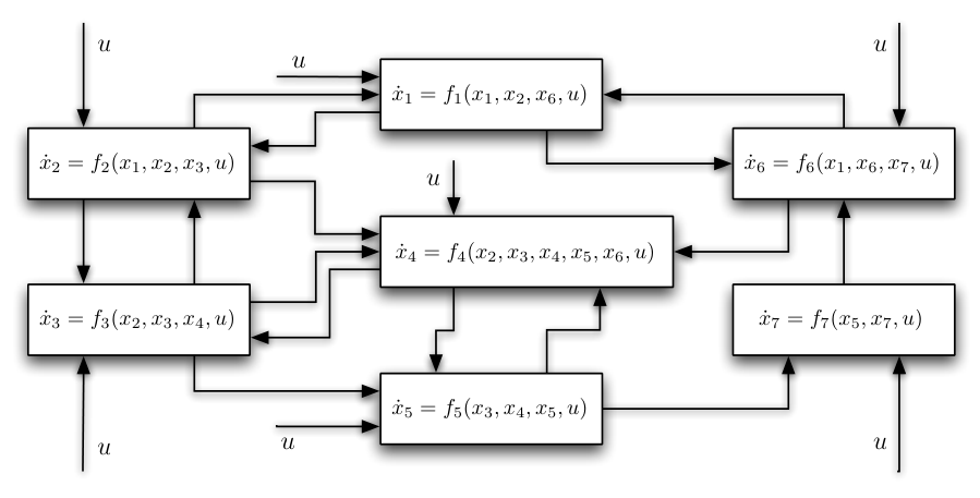
Associated to such a network is a directed graph, with vertices representing the subsystems and where the directed edges correspond to inputs going from system to system , see Figure 3. We will call the network strongly connected if its interconnection graph has the same property.
For networks of the type that has been just described we wish to construct Lyapunov functions as they are introduced now.
2.3 Stability
An appropriate stability notion to study nonlinear systems with inputs is input-to-state stability, introduced in [28]. The standard definition is as follows.
A forward complete system with is called input-to-state stable if there are , such that for all initial conditions and all we have
| (5) |
It is known to be an equivalent requirement to ask for the existence of an ISS Lyapunov function, [30]. These functions can be chosen to be smooth. For our purposes, however, it will be more convenient to have a broader class of functions available for the construction of a Lyapunov function. Thus we will call a function a Lyapunov function candidate, if the following assumption is met.
Assumption 1.
The function is continuous, proper and positive definite and locally Lipschitz continuous on .
Note that by Rademacher’s Theorem (e.g., [12, Theorem 5.8.6, p.281]) locally Lipschitz continuous functions on are differentiable almost everywhere in .
Definition 2.
We will call a function satisfying Assumption 1 an ISS Lyapunov function for , if there exist , and a positive definite function such that in all points of differentiability of we have
| (6) |
ISS and ISS Lyapunov functions are related in the expected manner:
Theorem 3.
A system is ISS if and only if it admits an ISS Lyapunov function in the sense of Definition 2.
This has been proved for smooth ISS Lyapunov functions in the literature [30]. So the hard converse statement is clear, as it is even possible to find smooth ISS Lyapunov functions, which satisfy Definition 2. The sufficiency proof for the Lipschitz continuous case goes along the lines presented in [30, 31] using the necessary tools from nonsmooth analysis, cf. [4, Theorem. 6.3].
Merely continuous ISS Lyapunov functions have been studied in [14, Ch. 3], arising as viscosity supersolutions to certain partial differential inequalities. Here we work with the Clarke generalized gradient of at . For functions satisfying Assumption 1 Clarke’s generalized gradient satisfies for that
| (7) |
An equivalent formulation to (6) is given by
| (8) |
Note that (8) is also applicable in points where is not differentiable.
2.4 Monotone aggregation
In this paper we concentrate on the construction of ISS Lyapunov functions for the interconnected system . For a single subsystem (3), in a similar manner to (6), we wish to quantify the combined effect of the inputs , , and on the evolution of the state . As we will see in the examples given in Section 3 it depends on the system under consideration how this combined effect can be expressed, through the sum of individual effects, using the maximum of individual effects or by other means. In order to be able to give a general treatment of this we introduce the notion of monotone aggregation functions (MAFs).
Definition 4.
A continuous function is called a monotone aggregation function if the following three properties hold
- (M1)
positivity: for all and if ;
- (M2)
strict increase11 1 Cf. Assumption (12), where for the purposes of this paper (M2) is further restricted.: if , then ;
- (M3)
unboundedness: if then .
The space of monotone aggregation functions is denoted by and denotes a vector , i.e., , for .
A direct consequence of (M2) and continuity is the weaker monotonicity property
- (M2’)
monotonicity: .
In [24, 25] MAFs have additionally been required to satisfy another property,
- (M4)
subadditivity: ,
which we do not need for the constructions provided in this paper, since we take a different approach, see Section 6.
Standard examples of monotone aggregation functions satisfying (M1)—(M4) are
On the other hand, the following function is not a MAF, since (M1) and (M3) are not satisfied; .
Using this definition we can define a notion of ISS Lyapunov function for systems with multiple inputs. In this case in (3) will have several gains corresponding to the inputs . For notational simplicity, we will include the gain throughout this paper. The following definition requires only Lipschitz continuity of the Lyapunov function.
Definition 5.
Consider the interconnected system (4) and assume that for each subsystem there is a given function satisfying Assumption 1.
For the function is called an ISS Lyapunov function for , if there exist , and a positive definite function such that at all points of differentiability of
| (9) |
The functions and are called ISS Lyapunov gains.
Several examples of ISS Lyapunov functions are given in the next section.
Let us call , , the internal inputs to and the external input. Note that the role of functions and is essentially to indicate whether there is any influence of different inputs on the corresponding state. In case does not depend on there is no influence of on the state of . In this case we define , in particular always . This allows us to collect the internal gains into a matrix
| (10) |
If we add the external gains as the last column into this matrix then we denote it by . The function describes how the internal and external gains interactively enter in a common influence on . The above definition motivates the introduction of the following nonlinear map
| (11) |
Similarly we define . The matrices and are from now on referred to as gain matrices, and as gain operators.
Remark 6 (general assumption).
Given and , we will from now on assume that and are compatible in the following sense: For each , let denote the set of indices corresponding to the nonzero entries in the th row of . Then it is understood that also the restriction of to the indices satisfies (M2), i.e.,
| (12) |
In particular we assume that the function
for satisfies (M2). Note that (M1) and (M3) are automatically satisfied.
The examples in the next section show explicitly how the introduced functions, matrices and operators may look like for some particular cases. Clearly, the gain operators will have to satisfy certain conditions if we want to be able to deduce that (4) is ISS with respect to external inputs, see Section 5.
3 Examples for monotone aggregation
In this section we show how different MAFs may appear in different applications, for further examples see [10]. We begin with a purely academic example and discuss linear systems and neural networks later in this section. Consider the system
| (13) |
where . Take as a Lyapunov function candidate. It is easy to see that if and then
if . The conditions and translate into and in terms of this becomes
This is a Lyapunov ISS estimate where the gains are aggregated using a maximum, i.e., in this case we can take and and .
Note that there is a certain arbitrariness in the choice of and . In the example one could as well take and , giving exactly the same condition, but different gains and a different monotone aggregation function. At the end of the day the small gain condition comes down to mapping properties of . Different choices of and may lead to the same operator . However, as we will see at a later stage, certain choices of can be computationally more convenient than others. In particular, if we can choose , the task of checking the small gain condition reduces to checking a cycle condition, cf. Section 8.4.
3.1 Linear systems
Consider linear interconnected systems
| (14) |
with and matrices of appropriate dimensions. Each system is ISS from to if and only if is Hurwitz. It is known that is Hurwitz if and only if for any given symmetric positive definite there is a unique symmetric positive definite solution of , see, e.g., [15, Cor. 3.3.47 and Rem. 3.3.48, p.284f]. Thus we choose the Lyapunov function , where is the solution corresponding to a symmetric positive definite . In this case, along trajectories of the autonomous system
we have
for , the smallest eigenvalue of . For system (14) we obtain
| (15) |
where the last inequality (15) is satisfied for a given if
| (16) |
with . To write this implication in the form (9) we note that . Let us denote , , then the inequality (16) is satisfied if
This way we see that the function is an ISS Lyapunov function for with gains given by
for , , and
for , and . Further we have
for and . This satisfies (M1), (M2), and (M3), but not (M4). By defining for we can write
and have
| (17) |
Interestingly, the choice of quadratic Lyapunov functions for the subsystems naturally leads to a nonlinear mapping with a useful homogeneity property, see Proposition 20.
3.2 Neural networks
As the next example consider a Cohen-Grossberg neural network as in [35]. The dynamics of each neuron is given by
| (18) |
, where denotes the state of the -th neuron and is a strictly positive amplification function. As in [35] we assume that the fixed point is shifted to the origin. Then the function typically satisfies the sign condition and satisfies furthermore for some . The activation function is typically assumed to be sigmoid. The matrix describes the interconnection of neurons in the network and is a given constant input from outside. However for our consideration we allow to be an arbitrary measurable function in .
In applications the matrix is usually the result of training using some learning algorithm and appropriate training data. The specifics depend on the type of network architecture and learning algorithm chosen and on the particular application. Such considerations are beyond the scope of the current paper. We simply assume that is given and concern ourselves solely with stability considerations.
Note that for any sigmoid function there exists a such that . Following [35] we assume , .
Recall the triangle inequality for -functions: For any and any it holds
We claim that is an ISS Lyapunov function for in (18). Fix an arbitrary function and some satisfying . Then by the triangle inequality we have
In this case we have
additive with respect to the external input and
The MAF satisfies (M1), (M2), and (M3). It satisfies (M4) if and only if is subadditive.
4 Monotone Operators and generalized small gain conditions
In Section 2.4 we saw that in the ISS context the mutual influence between subsystems (3) and the influence from external inputs to the subsystems can be quantified by the gain matrices and and gain operators and . The interconnection structure of the subsystems naturally leads to a weighted, directed graph, where the weights are the nonlinear gain functions, and the vertices are the subsystems. There is an edge from the vertex to the vertex if and only if there is an influence of the state on the state , i.e., there is a nonzero gain .
Connectedness properties of the interconnection graph together with mapping properties of the gain operators will yield a generalized small gain condition. In essence we need a nonlinear version of a Perron vector for the construction of a Lyapunov function for the interconnected system. This will be made rigorous in the sequel. But first we introduce some further notation.
The adjacency matrix of a matrix is defined by if and otherwise. Then is also the adjacency matrix of the graph representing an interconnection.
We say that a matrix is primitive, irreducible or reducible if and only if is primitive, irreducible or reducible, respectively. Recall (and see [2] for more on this subject) that a nonnegative matrix is
- •
primitive if there exists a such that is positive;
- •
irreducible if for every pair there exists a such that the th entry of is positive; obviously, primitivity implies irreducibility;
- •
reducible if it is not irreducible.
A network or a graph is strongly connected if and only if the associated adjacency matrix is irreducible, see also [2].
For functions we define a diagonal operator by
| (19) |
For an operator , the condition means that for all , . In words, at least one component of has to be strictly less than the corresponding component of .
Definition 7 (Small gain conditions).
It is not difficult to see that (sSGC) can equivalently be stated as
| (sSGC’) |
Also for (sSGC) or (sSGC’) to hold it is sufficient to assume that the function are all identical. This can be seen by defining . We abbreviate this in writing for some .
For maps we define the following sets:
If no confusion arises we will omit the reference to . Topological properties of the introduced sets are related to the small gain conditions (SGC), cf. also [5, 6, 25]. They will be used in the next section for the construction of an ISS Lyapunov function for the interconnection.
5 Lyapunov functions
In this section we present the two main results of the paper. The first is a topological result on the existence of a jointly unbounded path in the set , provided that satisfies the small gain condition. This path will be crucial in the construction of a Lyapunov function, which is the second main result of this section.
Definition 8.
A continuous path will be called an -path with respect to if
- (i)
for each , the function is locally Lipschitz continuous on ;
- (ii)
for every compact set there are constants such that for all and all points of differentiability of we have
(20) - (iii)
for all , i.e.
(21)
Now we can state the first of our two main results, which regards the existence of -paths.
Theorem 9.
Let be a gain matrix and . Assume that one of the following assumptions is satisfied
- (i)
is linear and the spectral radius of is less than one;
- (ii)
is irreducible and ;
- (iii)
and ;
- (iv)
alternatively assume that is bounded, i.e., , and satisfies .
Then there exists an -path with respect to .
We will postpone the proof of this rather topological result to Section 8 and reap the fruits of Theorem 9 first. Note, however, that for (iii) there exists a “”-type equivalent formulation, cf. Theorem 38 and see [21, 33, 6, 20].
In addition to the above result, the existence of -paths can also be asserted for reducible and with mixed, bounded and unbounded, class entries, see Theorem 36 and Proposition 37, respectively.
Theorem 10.
Consider the interconnected system given by (3), (4) where each of the subsystems has an ISS Lyapunov function , the corresponding gain matrix is given by (10), and is given by (9). Assume there are an -path with respect to and a function such that
| (22) |
is satisfied, then an ISS Lyapunov function for the overall system is given by
| (23) |
In particular, for all points of differentiability of we have the implication
| (24) |
where is a suitable positive definite function.
Note that by construction the Lyapunov function is not smooth, even if the functions for the subsystems are. This is why it is appropriate in this framework to consider Lipschitz continuous Lyapunov functions, which are differentiable almost everywhere.
Proof.
We will show the assertion in the Clarke gradient sense. For there is nothing to show. So let . Denote by the set of indices for which
| (25) |
Then , for . Also as is obtained through maximization we have because of [4, p.83] that
| (26) |
Fix and assume without loss of generality . Then if we assume it follows in particular that . Using the abbreviation , denoting the first component of by and using assumption (22) we have
where we have used (25) and (M2’) in the last inequality. Thus the ISS condition (9) is applicable and we have for all that
| (27) |
By the chain rule for Lipschitz continuous functions [4, Theorem 2.5] we have
Note that in the previous equation the number is bounded away from zero because of (20). We set for
where is the constant corresponding to the set given by (20) in the definition of an -path. With the convention we now define for
Here we have used that for a given and the norm of such that is bounded away from .
In the absence of external inputs, ISS is the same as 0-GAS (cf. [29, 30, 31]). We note the following consequence in the case that only global asymptotic stability is of interest.
Corollary 11 (0-GAS for strongly interconnected networks).
In the setting of Theorem 10, assume that the external inputs satisfy and that the network of interconnected systems is strongly connected. If then the network is 0-GAS.
Proof.
Remark 12.
At first sight it might seem that the previous corollary is stronger than [18, Cor. 2.1], as no robustness term is needed in the assumptions. However, the result here is formulated for Lyapunov functions whereas the result in [18] is based on the trajectory formulation of ISS in summation form. The proof in the trajectory version essentially requires bounds on , which relies heavily on unless , [18, 6, 24]. In contrast, for -GAS the is not needed in the Lyapunov setting, because for irreducible it is possible to construct the path without by Theorem 9 (ii).
We now specialize the Theorem 10 to particular cases of interest. Namely, when the gain with respect to the external input enters the ISS condition (i) additively, (ii) via maximization and (iii) as a factor.
Corollary 13 (Additive gain of external input ).
Consider the interconnected system given by (3), (4) where each of the subsystems has an ISS Lyapunov function and the corresponding gain matrix is given by (11). Assume that the ISS condition is additive in the gain of , that is,
| (29) |
where . If is irreducible and if there exists an such that for the gain operator satisfies the strong small gain condition
then the interconnected system is ISS and an ISS Lyapunov function is given by (23), where is an arbitrary -path with respect to .
Proof.
By Theorem 9 an -path exists. Observe that by irreducibility, (M1), and (M3) it follows that is unbounded in all components. Let be such that for all
Note that this is possible, because on the left we take the minimum of a finite number of functions. Then we have for all , that
Thus and the assertion follows from Theorem 10. ∎
Corollary 14 (Maximization w.r.t. external gain).
Consider the interconnected system given by (3), (4) where each of the subsystems has an ISS Lyapunov function and the corresponding gain matrix is given by (11). Assume that enters the ISS condition via maximization, that is,
| (30) |
where . Then, if is irreducible and satisfies the small gain condition
the interconnected system is ISS and an ISS Lyapunov function is given by (23), where is an arbitrary -path with respect to and is a function with the property
| (31) |
where denotes the -th row of .
Proof.
In the next result observe that (M3) is not always necessary for the -component of .
Corollary 15 (Separation in gains).
Consider the interconnected system given by (3), (4) where each of the subsystems has an ISS Lyapunov function and the corresponding gain matrix is given by (11). Assume that is irreducible and that the gains in the ISS condition are separated, that is, there exist , , and such that
| (32) |
If there exists an such that for the gain operator satisfies the strong small gain condition
then the interconnected system is ISS and an ISS Lyapunov function is given by (23), where is an arbitrary -path with respect to .
6 The reducible case and scaling
The results that have been obtained so far concern mostly strongly connected networks, that is, networks with an irreducible gain operator. Already in [27] it has been shown that cascades of ISS systems are ISS. Cascades are a special case of networks where the gain matrix is reducible. In this section we briefly explain how a Lyapunov function for a network that is not strongly connected may be constructed based on the construction for the strongly connected components of the network. Another approach would be to construct the -path for reducible operators as has been done in [25] using assumption (M4).
It is well known, that if the network is not strongly connected, or equivalently if the gain matrix is reducible, then may be brought in upper block triangular form via a permutation of the vertices of the network as in the nonnegative matrix case [2, 6]. After this transformation is of the form
| (33) |
where each of the blocks on the diagonal , , is either irreducible or . Let , with the convention that . We denote the states corresponding to the strongly connected components by
We will show that in order to obtain an overall ISS Lyapunov function it is sufficient to construct ISS Lyapunov functions for each of the irreducible blocks (where the respective states with higher indices are treated as inputs). The desired result is an iterative application of the following observation.
Lemma 16.
Let a gain matrix be given by
| (34) |
and let be defined by . Then there exist an -path and such that (22) holds.
Proof.
By construction the maps and are in . Choose a -function , such that satisfies the conditions (i) and (ii) in Definition 8. Define and . Then it is a straightforward calculation to check that the assertion holds. ∎
The result is now as follows.
Proposition 17.
Consider a simply connected interconnected system given by (3), (4) where each of the subsystems has an ISS Lyapunov function , the corresponding gain matrix is given by (10), and is given by (9). Assume that the gain matrix is in the reduced form (33). If for each there exists an ISS Lyapunov function for the state with respect to the inputs then there exists an ISS Lyapunov function for the state with respect to the input .
Proof.
By assumption for each there exist gain functions and and MAFs such that
We now argue by induction. If , there is nothing to show. If the result is shown for blocks, consider a gain matrix as in (33). By assumption there exists an ISS Lyapunov function such that
As the remaining part has only external inputs, we see that is of the form (34) and so Lemma 16 is applicable. This shows that the assumptions of Theorem 10 are met and so a Lyapunov function for the overall system is given by (23). ∎
It is easy to see that the assumption (or ) is equivalent to the requirement that the blocks on the diagonal satisfy the (strong) small gain condition (SGC)/(sSGC). Thus we immediately obtain the following statements.
Corollary 18 (Summation of gains).
Consider the interconnected system given by (3), (4) where each of the subsystems has an ISS Lyapunov function and the corresponding gain matrix is given by (11). Assume that the ISS condition is additive in the gains, that is,
| (35) |
If there exists an such that for the gain operator satisfies the strong small gain condition
then the interconnected system is ISS.
Proof.
Corollary 19 (Maximization of gains).
Consider the interconnected system given by (3), (4) where each of the subsystems has an ISS Lyapunov function and the corresponding gain matrix is given by (11). Assume that the gains enter the ISS condition via maximization, that is,
| (36) |
If the gain operator satisfies the small gain condition
then the interconnected system is ISS.
7 Applications of the general small gain theorem
In Section 3 we have presented several examples of functions , and gain operators , . Here we will show how our main results apply to these examples. Before we proceed, let us consider the special case of homogeneous (of degree 1) [13]. Here is homogeneous of degree one if for any and any we have .
Proposition 20 (Explicit paths and Lyapunov functions for homogeneous gain operators).
Let in (2) be a strongly connected network of subsystems (1) and , be the corresponding gain operators. Let be homogeneous and let satisfy one of the conditions (35), (36), or (32). If satisfies the strong small gain condition (sSGC) ((SGC) in case of (36)) then the interconnection is ISS, moreover there exists a (nonlinear) eigenvector of such that with and an ISS Lyapunov function for the network is given by
| (37) |
Proof.
First note that one of the Corollaries 18, 19, or 15 can be applied and the ISS property follows immediately. By the assumptions of the proposition we have an irreducible monotone homogeneous operator on the positive orthant . By the generalized Perron-Frobenius Theorem [13] there exists a positive eigenvector . Its eigenvalue is less than one, otherwise we have a contradiction to the small gain condition. The ray defined by this vector is a corresponding -path and by Theorem 10 we obtain (37). ∎
One type of homogeneous operators arises from linear operators through multiplicative coordinate transforms. In this case we can further specialize the assumptions of the previous result.
Lemma 21.
Let satisfy22 2 In other words, for some . for all . Let , , and be given by
Then is homogeneous. Moreover, if and only if the spectral radius of is less than one.
Proof.
If the spectral radius of is less than one, then there exists a positive vector satisfying : Just add a small to every entry of , so that the spectral radius of is still less than one, due to continuity of the spectrum. Then there exists a Perron vector such that . Define and observe that . Then we have
| (38) | ||||
for all . So an -path for is given by for . Existence of an -path implies the small gain condition: The origin in is globally attractive with respect to the system , as can be seen by a monotonicity argument. By [6, Theorem 23] or [25, Prop. 4.1] we have .
Assuming that the spectral radius of is greater or equal to one there exists , , such that . Defining we have . Hence if and only if the spectral radius of is less than one.
Homogeneity of is obtained as in (38). ∎
7.1 Application to linear interconnected systems
Proposition 22.
Let each in (14) be ISS with a quadratic ISS Lyapunov function , so that the corresponding operator can be taken to be as in (17). If the spectral radius of the associated matrix
| (39) |
is less than 1, then the interconnection
is ISS and its (nonsmooth) ISS Lyapunov function can be taken as
for some positive vector .
Proof.
We have , where for . Now satisfies the assumptions of Lemma 21, which yields that satisfies the small gain condition if and only if . If or equivalently is irreducible then there exists by Proposition 20 an such that . By (17) we see, that there exists an such that . Then defining we obtain for all that
Thus the conditions of Theorem 10 are satisfied and an ISS Lyapunov function can be taken as .
If is reducible the previous construction has to be performed for every irreducible blocks and then the scaling techniques of Section 6 need to be applied. ∎
7.2 Application to neural networks
Consider the neural network (18) discussed in Section 3.2. This is a system of coupled nonlinear equations, and we have seen that each subsystem is ISS. Note that so far we have not imposed any restrictions on the coefficients . Moreover the assumptions imposed on are essentially milder then in [35]. However to obtain the ISS property of the network we need to require more. The small gain condition can be used for this purpose. It will impose restrictions on the coupling terms . From Corollary 13 it follows:
Theorem 23.
Remark 24.
In [35] the authors have proved that there exists a unique equilibrium point for the network and given constant external inputs. They have also proved the exponential stability of this equilibrium. We have considered arbitrary external inputs to the network and proved the ISS property for the interconnection.
8 Path construction
This section explains the relation between the small gain condition for and its mapping properties. Then we construct a strictly increasing -path and prove Theorem 9 and some extensions. Let us first consider some simple particular cases to explain the main ideas, as depicted in Figure 4. In the following subsections we then proceed to the main path construction results.
A map is monotone if implies . Clearly any matrix together with an aggregation induces a monotone map .
Lemma 25.
Let and , such that satisfies (SGC). If , then .
Proof.
If , then and by monotonicity . By induction is a monotonically decreasing sequence bounded from below by . Thus exists and by continuity we have . By the small gain condition it follows . ∎
Lemma 26.
Assume that has no zero rows and let . If , then
- (i)
- (ii)
for all the convex combination .
Proof.
(i) By assumption and so by the monotonicity assumption (M2) we have . Furthermore, as and the matrix has no zeros rows, we have that by assumption (M1).
Lemma 27.
Assume that has no zero rows and let be such that satisfies the small gain condition (SGC). Let . Then there exists a path in connecting the origin and .
Proof.
The following result applies to whose entries are bounded, i.e., in .
Proposition 28.
Assume that has no zero rows and let be such that satisfies the small gain condition (SGC). Assume furthermore that is bounded, then there exists an -path with respect to .
Proof.
By assumption the set is bounded, so pick . Then clearly, and so . By the same argument for all . Thus a path in through the point exists, if we find a path from to contained in . The remainder of the result is given by Lemma 27. ∎
The difficulty now arises if happens to be unbounded, i.e., contains entries of class . In the unbounded case the simple construction above is not possible. In the following we will first consider the case that all nonzero entries of are of class . Beforehand we introduce a few technical lemmas.
8.1 Technical lemmas
Throughout this subsection denotes a continuous, monotone map, i.e., satisfies whenever . We start with a few observations.
Lemma 29.
Let . Then there exists a such that .
Proof.
Just define . Then , which proves the lemma. ∎
Lemma 30.
- (i)
Let for some such that . Then for any there exist satisfying , such that for , ,
Moreover, , , can be chosen such that for all we have
- (ii)
Let for some . Then there exist , such that for , ,
For maps define the decay set
where we again omit the reference to if this is clear from the context.
Lemma 31.
Let be monotone and for some . Then
- (i)
for all ;
- (ii)
, if satisfies whenever ; the same is true for replaced by ;
The proofs of the lemmas are simple and thus omitted for reasons of space. Nevertheless they can be found in [24, p.10, p.29].
We will need the following connectedness property in the sequel.
Proposition 32.
Let and be such that satisfies the small gain condition (SGC). Then is nonempty and pathwise connected. Moreover, if satisfies whenever , then for any there exists a strictly increasing -path connecting and .
Proof.
Note that always , hence cannot be empty. Along the lines the proof of Lemma 27 it follows that each point in is pathwise connected to the origin. ∎
Another crucial step, which is of topological nature, regards preimages of points in the decay set . In general it is not guaranteed, that for with , we also have . The set of points in for which preimages of arbitrary order are also in is the set
Of course, this set might be empty or bounded. We will use it to construct -paths for operators satisfying the small gain condition.
Proposition 33 ([25, Prop. 5.4]).
Let be monotone and continuous and satisfy for all . Assume that satisfies the property
| (40) |
as for any sequence .
Then , for all , and is unbounded.

A result based on the topological fixed point theorem due to Knaster, Kuratowski, and Mazurkiewicz allows to relate and the small gain condition. It is essential for the proof of Proposition 33.
Proposition 34.
Let be monotone and continuous. If for all then the set is nonempty for all .
8.2 Paths for gain matrices
In this subsection we consider matrices , i.e., all nonzero entries of are assumed to be unbounded functions.
In this setting we assume and utilize that the graph associated to is strongly connected, i.e., is irreducible. So that if we consider powers , for each components and there exists a such that is an unbounded function.
Theorem 35.
Let be irreducible, , and assume . Then there exists a strictly increasing path satisfying
The main technical difficulty in the proof is to construct the path in the unbounded direction, the other case has already been dealt with in Proposition 32.
The proof comprises the following steps: First due to [25, Prop. 5.8] we may choose a function so that for we have . Then we construct a monotone (but not necessarily strictly monotone) sequence in , satisfying , so that each component sequence is unbounded. At this point a linear interpolation of the sequence points may not yield a strictly increasing path. So finally we use the “extra space” provided by in the set to obtain a strictly increasing sequence in which we can linearly interpolate to obtain the desired -path.
Proof.
Since is irreducible, it has no zero rows and hence satisfies whenever . By [25, Prop. 5.8] there exists a so that for we have . Now we construct a nondecreasing sequence in :
Let . Then and by induction also all powers , , satisfy (40).
By Proposition 33 the set is unbounded, so we may pick an . We can actually choose , since the sequence we are going to construct will be unbounded in every component, at which point we may replace by some for large enough.
Due to irreducibility of (and Remark 6) the following property holds: For any pair there exists an such that
| (41) |
is an unbounded and increasing function, where is the -th unit vector. By monotonicity the same holds when is considered instead of . Now define a sequence by choosing
for . This is possible, since by definition is backward invariant under .
This sequence satisfies by definition. We claim that it is unbounded, and also unbounded in every component: To this end assume first that it is bounded. Then by monotonicity there exists a limit . By continuity of and since we have
contradicting for all . Hence the sequence must be unbounded.
Let be an index such that is unbounded, let be arbitrary and choose such that the function in (41) is unbounded for . Choose real numbers such that for all . Then we have
As the term on the left goes to for , so does . Hence is unbounded in every component.
Now by Lemma 31(ii) the sequence is contained in , but it may not be strictly increasing, as we only know for all . We define a strictly increasing sequence as follows: By Lemma 30 for any we may factorize so that and for all and all . Using this factorization we define
for all . By the definition of , this sequence is clearly strictly increasing and inherits from the unboundedness in all components.
We claim that : This follows from
Now we prove that for we have . Clearly
and application of the strictly increasing operator yields
Hence .
Now we may define as a parametrization of the linear interpolation of the points in the unbounded direction and utilize the construction from Lemma 27 for the other direction. Clearly this function is an -path as it has component functions of class and is piecewise linear on every compact interval contained in . ∎
It is possible to consider the reducible case in a similar fashion. The argument is essentially an induction over the number of irreducible and zero blocks on the diagonal of the reducible operator. We cite the following result from [25, Theorem 5.10]. However, for the construction of an ISS Lyapunov function in the case of reducible , we take a different route as described in Section 6, thus avoiding the use of assumption (M4).
Theorem 36.
Let be reducible, satisfying (M4), for some , and assume . Then there exists a monotone and continuous operator and a strictly increasing path whose component functions are all unbounded, such that .
8.3 General
In the preceding subsections we have seen that it is possible to construct -paths for matrices whose nonzero entries are either all bounded, or all unbounded. It remains to consider the case that the nonzero entries of are partly of class and partly of class . We can state the following result.
Proposition 37.
Let and let satisfy (M4). Assume satisfies (sSGC). Then there exists an -path for .
Proof. Write
with , . Clearly we have and and hence both maps satisfy
where serves as a placeholder for the subscripts and .
The map is bounded. Hence is a finite vector.
By Theorem 36. for there exists a function and a -path so that for the diagonal operator we have
Similarly, by Proposition 28, there exists a -path such that for all . In fact, and this is the key to this proof, it is possible to choose in the region where to grow arbitrarily slowly: For any we can find a , such that
e.g., by choosing satisfying . This is always possible. Denote , (so that ) and choose , such that . Then after reparametrization we may assume that
for all . Using Lemma 27, we let be a finite-length path satisfying
Now define by
It remains to check that satisfies for . Indeed, for we have
where the last inequality is due to (M4). This completes the proof.
8.4 Special case: Maximization
The case when the aggregation is the maximum, i.e., , is indeed a special case, since not only the small gain condition can be formulated in simpler manner, but also the path construction can be achieved without the need of the diagonal operator as before.
A cycle in a matrix is finite sequence of nonzero entries of of the form
A cycle is called subordinated if , and it is called a contraction, if
It is an easy exercise to show that when all subordinated cycles are contractions then already all cycles are contractions.
Theorem 38.
Let and . If all subordinated cycles of are contractions, then there exists an -path with respect to .
The proof is composed of the following steps. The first step is to show that the cycle condition (all cycles being contractions) is equivalent to . Note that automatically satisfies (M4), but (M4) is actually not needed for the proof. Then the path-construction can essentially be done as before, replacing sums by maximization, and one can even avoid the use of . Cf. also[25].
8.5 Proof of Theorem 9
We now come to the easiest part of this section, which is to combine all the preceding results to one general theorem for matrices with entries of class , namely Theorem 9.
Proof of Theorem 9.
9 Remarks for the case of three subsystems
Recall that a construction of an -path for the case of two subsystem was given in [17]. We have seen that in a general case of subsystems the construction involves more theory and topological properties of that follow from the small gain condition. However in case of three subsystems can be found by rather simple considerations. Here we provide this illustrative construction. Let us consider the special case , , , and for simplicity assume that for all , so that
| (42) |
Fix , then it follows that there is exactly one satisfying
| (43) |
since, for a fixed the left side of (43) is a strictly decreasing function of while the right side of (43) is strictly increasing one. The small gain condition (42) in particular assures that for any . Let be the solution of and be the solution of then
Hence the root of the left side of (43) is greater than the root of the right side of (43). This proves that for any there is always exactly one satisfying (43), see Figure 6.
By the continuity and monotonicity of it follows that depends continuously on and is strictly increasing with . We can define for and to be the unique solving (43) for .
Denote and , and define Let us show that for all . If this is not true then there exists such that holds. Consider the point Then , , and . In other words,
contradicting (3). Hence is not empty for all .
Consider the functions and . The question is how to choose such that . Note that . Let , so that for all . Since is unbounded, for all the set is compact and for all points the relation holds. We have for all where is a (not necessarily strictly) increasing function. Now take and observe that and for all . Hence satisfies for all .
The case where one of is not a function but zero can be treated similarly.
10 Conclusions
In this paper we have provided a method for the construction of ISS Lyapunov functions for interconnections of nonlinear ISS systems. The method applies for an interconnection of an arbitrary finite number of subsystems interconnected in an arbitrary way and satisfying a small gain condition. The small gain condition is imposed on the nonlinear gain operator that we have introduced here. This operator contains the information of the topological structure of the network and the interactions between its subsystems. An ISS Lyapunov function for such a network is given in terms of ISS Lyapunov functions of subsystems and some auxiliary functions. We have shown how this construction is related to the small gain condition and mapping properties of the gain operator and its invariant sets. Namely the small gain condition guarantees the existence of an unbounded vector function with path in an invariant set of the operator . This auxiliary function can be used to rescale the ISS Lyapunov functions of the individual subsystems and aggregate them into an ISS Lyapunov function for the entire network. The construction technique for this vector function has been detailed as well as the construction of the composite Lyapunov function. The constructed Lyapunov function is only locally Lipschitz continuous, so that methods from nonsmooth analysis had to be used. The proposed method has been exemplified for linear systems and neural networks.
References
- [1] V. Andrieu, L. Praly, and A. Astolfi, Asymptotic tracking of a state trajectory by output-feedback for a class of non linear systems, in Proc. of 46th IEEE Conference on Decision and Control, CDC 2007, New Orleans, LA, December 2007, pp. 5228–5233.
- [2] A. Berman and R. J. Plemmons, Nonnegative matrices in the mathematical sciences, Academic Press, New York, 1979.
- [3] Anna L. Chen, Gui-Qiang Chen, and R. A. Freeman, Stability of nonlinear feedback systems: a new small-gain theorem, SIAM J. Control Optim., 46 (2007), pp. 1995–2012.
- [4] F. H. Clarke, Yu. S. Ledyaev, R. J. Stern, and P. R. Wolenski, Nonsmooth analysis and control theory, Springer, 1998.
- [5] S. Dashkovskiy, B. Rüffer, and F. Wirth, A small-gain type stability criterion for large scale networks of ISS systems, in 44th IEEE Conference on Decision and Control and European Control Conference CDC/ECC 2005, Seville, Spain, December 2005, pp. 5633–5638.
- [6] , An ISS small-gain theorem for general networks, Mathematics of Control, Signals, and Systems, 19 (2007), pp. 93–122.
- [7] , A Lyapunov ISS small gain theorem for strongly connected networks, in Proc. 7th IFAC Symposium on Nonlinear Control Systems, NOLCOS2007, Pretoria, South Africa, August 2007, pp. 283–288.
- [8] S. Dashkovskiy, Björn S. Rüffer, and Fabian R. Wirth, An ISS Lyapunov function for networks of ISS systems, in Proceedings of the 17th International Symposium on Mathematical Theory of Networks and Systems (MTNS), Kyoto, Japan, July 24–28 2006, pp. 77–82.
- [9] S. N. Dashkovskiy, B. S. Rüffer, and F. R. Wirth, Numerical verification of local input-to-state stability for large networks, in Proc. of 46th IEEE Conference on Decision and Control, CDC 2007, New Orleans, LA, December 2007, pp. 4471–4476.
- [10] , Applications of the general Lyapunov ISS small-gain theorem for networks, in Proceedings of the 47th IEEE Conference on Decision and Control CDC 2008, Cancun, Mexico, Dec. 9–11 2008, pp. 25–30.
- [11] B. C. Eaves, Homotopies for computation of fixed points, Math. Programming, 3 (1972), pp. 1–22.
- [12] L. C. Evans, Partial differential equations, vol. 19 of Graduate Studies in Mathematics, American Mathematical Society, Providence, RI, 1998.
- [13] S. Gaubert and J. Gunawardena, The Perron-Frobenius theorem for homogeneous, monotone functions, Trans. Amer. Math. Soc., 356 (2004), pp. 4931–4950 (electronic).
- [14] L. Grüne, Input-to-state dynamical stability and its Lyapunov function characterization, IEEE Trans. Automat. Control, 47 (2002), pp. 1499–1504.
- [15] D. Hinrichsen and A. J. Pritchard, Mathematical Systems Theory I — Modelling, State Space Analysis, Stability and Robustness, Springer, 2005.
- [16] , Composite systems with uncertain couplings of fixed structure: scaled Riccati equations and the problem of quadratic stability, SIAM J. Control Optim., 47 (2008), pp. 3037–3075.
- [17] Zhong-Ping Jiang, I. M. Y. Mareels, and Yuan Wang, A Lyapunov formulation of the nonlinear small-gain theorem for interconnected ISS systems, Automatica J. IFAC, 32 (1996), pp. 1211–1215.
- [18] Z.-P. Jiang, A. R. Teel, and L. Praly, Small-gain theorem for ISS systems and applications, Math. Control Signals Systems, 7 (1994), pp. 95–120.
- [19] Zhong-Ping Jiang and Yuan Wang, A generalization of the nonlinear small-gain theorem for large-scale complex systems, in Proc. 7th World Congress on Intelligent Control and Automation, June 2008, pp. 1188–1193.
- [20] I. Karafyllis and Zhong-Ping Jiang, A vector small-gain theorem for general nonlinear control systems, Submitted to IEEE Trans. Automat. Control, (5 April 2009). arXiv:0904.0755v1.
- [21] H. G. Potrykus, F. Allgöwer, and S. Joe Qin, The character of an idempotent-analytic nonlinear small gain theorem, in Positive systems (Rome, 2003), vol. 294 of Lecture Notes in Control and Inform. Sci., Springer, Berlin, 2003, pp. 361–368.
- [22] D.M. Raimondo, L. Magni, and R. Scattolini, Decentralized MPC of nonlinear systems: An input-to-state stability approach, International Journal of Robust and Nonlinear Control, 17 (2007), pp. 1651–1667.
- [23] N. Rouche, P. Habets, and M. Laloy, Stability theory by Liapunov’s direct method, Springer, New York, 1977.
- [24] B. S. Rüffer, Monotone dynamical systems, graphs, and stability of large-scale interconnected systems, PhD thesis, Fachbereich 3, Mathematik und Informatik, Universität Bremen, Germany, 2007. Available online at http://nbn-resolving.de/urn:nbn:de:gbv:46-diss000109058.
- [25] , Monotone inequalities, dynamical systems, and paths in the positive orthant of Euclidean -space, Positivity, (2009). To appear, DOI 10.1007/s11117-009-0016-5.
- [26] D. D. Šiljak, Decentralized control of complex systems, vol. 184 of Mathematics in Science and Engineering, Academic Press Inc., Boston, MA, 1991.
- [27] E. Sontag and A. Teel, Changing supply functions in input/state stable systems, IEEE Trans. Automat. Control, 40 (1995), pp. 1476–1478.
- [28] E. D. Sontag, Smooth stabilization implies coprime factorization, IEEE Trans. Automat. Control, 34 (1989), pp. 435–443.
- [29] E. D. Sontag and Yuan Wang, On characterizations of input-to-state stability with respect to compact sets, in Proceedings of IFAC Non-Linear Control Systems Design Symposium, (NOLCOS ’95), Tahoe City, CA, June 1995, 1995, pp. 226–231.
- [30] , On characterizations of the input-to-state stability property, Systems Control Lett., 24 (1995), pp. 351–359.
- [31] , New characterizations of input-to-state stability, IEEE Trans. Automat. Control, 41 (1996), pp. 1283–1294.
- [32] A. R. Teel, A nonlinear small gain theorem for the analysis of control systems with saturation, IEEE Trans. Automat. Control, 41 (1996), pp. 1256–1270.
- [33] , Input-to-state stability and the nonlinear small gain theorem. Private communication, 2005.
- [34] M. Vidyasagar, Input-output analysis of large-scale interconnected systems, vol. 29 of Lecture Notes in Control and Information Sciences, Springer, Berlin, 1981.
- [35] Lin Wang and Xingfu Zou, Exponential stability of Cohen-Grossberg neural networks, Neural networks, 15 (2002), pp. 415–422.
- [36] G. Zames, On input-output stability of time-varying nonlinear feedback systems I. Conditions derived using concepts of loop gain conicity and positivity, IEEE Transactions on Automatic Control, 11 (1966), pp. 228–238.