跳到论文正文
W Papers独立论文阅读器 arXiv:0901.1705 论文正文 计算阅读时间 · 0%
引用这篇论文根据当前论文元数据生成,正式投稿前建议核对。


License: arXiv.org perpetual non-exclusive license
arXiv:0901.1705v2 [cs.IT] 18 Apr 2010

Rate Distortion with Side-Information at Many Decoders

Roy Timo    Terence Chan    Alex Grant ††thanks: This work was funded by the Australian Research Council Grant DP0880223.††thanks: R. Timo, T. Chan and A. Grant are with the Institute for Telecommunications Research, University of South Australia. Email: {roy.timo, terence.chan, alex.grant}@unisa.edu.au.
Abstract

We present a new inner bound for the rate region of the tt-stage successive-refinement problem with side-information. We also present a new upper bound for the rate-distortion function for lossy-source coding with multiple decoders and side-information. Characterising this rate-distortion function is a long-standing open problem, and it is widely believed that the tightest upper bound is provided by Theorem 2 of Heegard and Berger’s paper “Rate Distortion when Side Information may be Absent,” IEEE Trans. Inform. Theory, 1985. We give a counterexample to Heegard and Berger’s result.

Index Terms: 
Rate distortion, side-information, successive refinement.

I Introduction

One of the most important and celebrated results in multi-terminal information theory is Wyner and Ziv’s solution to the problem of lossy source coding with side-information at the decoder [1] – the Wyner-Ziv problem (fig. 1). The main objective of this problem is to find a computable characterisation [2, Pg. 259] of the rate-distortion function R⁡(d)R(d). This function describes the smallest rate at which the encoder can compress an iid random sequence 𝐗\mathbf{X} so that the decoder, which has side-information 𝐘\mathbf{Y}, can produce a replica 𝐗^\hat{\mathbf{X}} of 𝐗\mathbf{X} that satisfies the average distortion constraint

𝔼⁡[1n​∑i=1nδ⁡(Xi,X^i)]≤d,\mathbb{E}\left[\frac{1}{n}\sum_{i=1}^{n}\delta\big(X_{i},\hat{X}_{i}\big)\right]\leq d\ , (1)

where δ\delta is a real-valued distortion measure [3] and 𝔼⁡[⋅]\mathbb{E}[\cdot] is the expectation operation. In [1, Thm. 1], Wyner and Ziv famously showed that

R⁡(d)\displaystyle R(d) =minU⁡{I⁡(X,U)−I⁡(U,Y)},\displaystyle=\min_{U}\big\{I(X;U)-I(U;Y)\big\}\ , (2)

where the minimization is taken over all choices of an auxiliary random variable UU that is jointly distributed with (X,Y)(X,Y) and which satisfies the following two properties: (1) UU is conditionally independent of YY given XX; and (2) there exists a function X^​(U,Y)\hat{X}(U,Y) with 𝔼​δ​(X,X^​(U,Y))≤d\mathbb{E}\delta(X,\hat{X}(U,Y))\leq d.

In this paper, we study the following two extensions of the Wyner-Ziv problem: (1) the Wyner-Ziv problem with multiple decoders (fig. 3); and (2) the successive-refinement problem with side-information (fig. 4). A brief history of the literature on these problems is as follows.

Refer to caption
Fig. 1: The Wyner-Ziv Problem: (𝐗CLOSE,(\mathbf{X}, OPEN𝐘)\mathbf{Y}) == (X1CLOSE,(X_{1}, OPENY1)Y_{1}), (X2CLOSE,(X_{2}, OPENY2)Y_{2}), …\ldots, (XnCLOSE,(X_{n}, OPENYn)Y_{n}) is an iid random sequence emitted by a source q⁡(x,y)=Pr​[X=x,Y=y]q(x,y)=\text{Pr}[X=x,Y=y]. The encoder maps 𝐗\mathbf{X} to an index MM, which belongs to a finite set ℳ\mathscr{M}, at a rate rr. Using MM and 𝐘\mathbf{Y}, the decoder is required to generate a replica 𝐗^=X^1,X^2,…,X^n\hat{\mathbf{X}}=\hat{X}_{1},\hat{X}_{2},\ldots,\hat{X}_{n} of 𝐗\mathbf{X} to within an average distortion dd, according to (1). The rate-distortion function R⁡(d)R(d) is defined as the smallest rate for which such a reconstruction is possible. A single-letter expression for this function was first given in [1, Thm. 1].

I-A The Wyner-Ziv Problem with tt-Decoders

Suppose that the side-information 𝐘\mathbf{Y} in Figure 1 is unreliable in the sense that it may or may not be available to the decoder. If the encoder does not know a priori when 𝐘\mathbf{Y} is available, then Wyner and Ziv’s coding argument for (2) fails, and a more sophisticated argument is required to exploit 𝐘\mathbf{Y}. This observation inspired Kaspi [4] in 1980 (published by Wyner on behalf of Kaspi in 1994) as well as Heegard and Berger [5] in 1985 to independently study the problem shown in fig. 2 – the Kaspi/Heegard-Berger problem. As with the Wyner-Ziv problem, the objective of this problem is to characterise the corresponding rate-distortion function R⁡(d1,d2)R(d_{1},d_{2}). That is, to find the smallest rate such that decoders 1 and 2 can produce replicas 𝐗^1\hat{\mathbf{X}}_{1} and 𝐗^2\hat{\mathbf{X}}_{2} of 𝐗\mathbf{X} to within average distortions d1d_{1} and d2d_{2}, respectively. To this end, Heegard and Berger [5, Thm. 1] showed that11 1 Kaspi’s result, [4, Thm. 2], gives an alternative characterisation of R⁡(d1,d2)R(d_{1},d_{2}) that uses one auxiliary random variable.

R(d1,d2)=minU,W{I(X;W)+I(X;U∣Y,W)},R(d_{1},d_{2})=\min_{U,W}\big\{I\left(X;W\right)+I\left(X;U\mid Y,W\right)\big\}\ ,

where the minimization is taken over all choices of two auxiliary random variables, UU and WW, that are jointly distributed with (X,Y)(X,Y) and which satisfy the following two properties: (1) (U,W)(U,W) is conditionally independent of YY given XX; and (2) there exist functions X^1​(W)\hat{X}_{1}(W) and X^2​(Y,U,W)\hat{X}_{2}(Y,U,W) with 𝔼​δ​(X,X^1​(W))≤d1\mathbb{E}\delta(X,\hat{X}_{1}(W))\leq d_{1} and 𝔼​δ​(X,X^2​(Y,U,W))≤d2\mathbb{E}\delta(X,\hat{X}_{2}(Y,U,W))\leq d_{2}, respectively.

Refer to caption
Fig. 2: The Kaspi/Heegard-Berger Problem: The encoder compresses 𝐗\mathbf{X} in a manner suitable for two decoders – one of which has side-information 𝐘\mathbf{Y}. The rate-distortion function R⁡(d)R(d) defines the smallest rate at which decoders 1 and 2 can generate replicas 𝐗^1=X^1,1,X^1,2,…,X^1,n\hat{\mathbf{X}}_{1}=\hat{X}_{1,1},\hat{X}_{1,2},\ldots,\hat{X}_{1,n} and 𝐗^2=X^2,1,X^2,2,…,X^2,n\hat{\mathbf{X}}_{2}=\hat{X}_{2,1},\hat{X}_{2,2},\ldots,\hat{X}_{2,n} of 𝐗\mathbf{X} to within average distortions d1d_{1} and d2d_{2}, respectively. A single-letter expression for this function was independently given in [4] and [5].

The Kaspi/Heegard-Berger problem in Figure 2 was further generalised by Heegard and Berger in [5, Sec. VII] to the problem shown in Figure 3. There are tt-decoders, each with different side-information, and the objective is to characterise the corresponding rate-distortion function R⁡(𝐝)R(\mathbf{d}). Unfortunately, this function has eluded characterisation for all but a few special cases. For example, Heegard and Berger [5, Thm. 3] have characterised R⁡(𝐝)R(\mathbf{d}) for stochastically degraded side-information22 2 The joint probability distribution of (XCLOSE,(X, Y1,Y_{1}, Y2,Y_{2}, …,\ldots, OPENYt)Y_{t}) can be manipulated to form the Markov chain X⦵Yt⦵Yt−1⦵⋯⦵Y1X\minuso Y_{t}\minuso Y_{t-1}\minuso\cdots\minuso Y_{1} without altering R⁡(𝐝)R(\mathbf{d}). We discuss this problem in detail in Section II-C.; Tian and Diggavi [6, 7] have characterised R⁡(𝐝)R(\mathbf{d}) for a quadratic Gaussian source with jointly Gaussian side-information; and Sgarro’s result [8, Thm. 1] subsumes the corresponding lossless problem. Notwithstanding this difficulty, however, this problem has helped stimulate a number of important results [4, 9, 10, 7, 6].

Refer to caption
Fig. 3: The Wyner-Ziv problem with tt-decoders. The encoder compresses 𝐗\mathbf{X} in a manner suitable for tt-decoders – each of which has different side-information. The rate-distortion function R⁡(𝐝)R(\mathbf{d}), where 𝐝=(d1,d2,…,dt)\mathbf{d}=(d_{1},d_{2},\dots,d_{t}), defines the smallest rate at which decoder ll, for all l=1,2,…,tl=1,2,\ldots,t, can generate a replica 𝐗^l\hat{\mathbf{X}}_{l} of 𝐗\mathbf{X} to within an average distortion dld_{l}. This problem is open for t≥2t\geq 2. We present an upper bound for R⁡(𝐝)R(\mathbf{d}) in Theorem 2.

In [5, Thm. 2], Heegard and Berger claimed that a certain functional, R0​(𝐝)R_{0}(\mathbf{d}), is an upper bound for R⁡(𝐝)R(\mathbf{d}). (The expression for R0​(𝐝)R_{0}(\mathbf{d}) is given in equation (4) of Section II; however, this expression requires notation from Section II.) For twenty-five years, R0​(𝐝)R_{0}(\mathbf{d}) has been universally considered to be the tightest upper bound for R⁡(𝐝)R(\mathbf{d}) in the literature. In Example 3 of Section II, we present a counterexample to [5, Thm. 2] that shows R0​(𝐝)R_{0}(\mathbf{d}) is not an upper bound for R⁡(𝐝)R(\mathbf{d}). The invalidity of [5, Thm. 2] is by no means obvious as it involves a difficult minimization over (2t−1)(2^{t}-1)-auxiliary random variables. Indeed, we note that this theorem has been cited with modest frequency in the literature, and all the while this error appears to have gone unnoticed. We present a new upper bound for R⁡(𝐝)R(\mathbf{d}) in Theorem 2 of Section IV.

I-B The Successive-Refinement Problem with Side-Information

The aforementioned counterexample led us to study the tt-stage (or, tt-decoder) successive-refinement problem shown in Figure 4. The encoder maps 𝐗\mathbf{X} to tt indices: M1,M2,…,MtM_{1},M_{2},\dots,M_{t}. It is required that decoder ll uses indices M1M_{1} through MlM_{l} together with its side-information 𝐘l\mathbf{Y}_{l} to produce a replica 𝐗^l=Xl,1,Xl,2,…,Xl,n\hat{\mathbf{X}}_{l}=X_{l,1},X_{l,2},\ldots,X_{l,n} of 𝐗\mathbf{X} to within an average distortion dld_{l}. The objective of this problem is to characterise the resulting admissible-rate region ℛ⁡(𝐝)\mathscr{R}(\mathbf{d}). That is, to determine the set of all rate tuples 𝐫=(r1,r2,…,rt)\mathbf{r}=(r_{1},r_{2},\ldots,r_{t}) for which each decoder can reconstruct 𝐗\mathbf{X} to within its desired distortion level.

Refer to caption

Fig. 4: The successive-refinement problem with tt stages. The encoder compresses 𝐗\mathbf{X} in tt-stages. At stage ll, decoder ll generates a replica 𝐗^l\hat{\mathbf{X}}_{l} of 𝐗\mathbf{X}. This problem is open for t≥2t\geq 2. We present an inner bound for the admissible-rate region in Section III (Theorem 1).

Assuming the side-information is stochastically degraded, Steinberg and Merhav [9] characterised ℛ⁡(d1,d2)\mathscr{R}(d_{1},d_{2}) for t=2t=2 decoders. Shortly thereafter, Tian and Diggavi [6] extended this problem to tt-decoders and proved the following result.

Proposition 1

If the side-information is stochastically degraded, then ℛ⁡(𝐝)\mathscr{R}(\mathbf{d}) is equal to the set of all rate tuples 𝐫\mathbf{r} for which there exists tt auxiliary random variables U1U_{1}, U2U_{2}, …\ldots, UtU_{t} such that

∑k=1lrk≥∑k=1lI(X;Uk|U1,U2,…,Uk−1,Yk),\sum_{k=1}^{l}r_{k}\geq\sum_{k=1}^{l}I\big(X;U_{k}\big|U_{1},U_{2},\ldots,U_{k-1},Y_{k}\big)\ ,

for all l=1,2,…,tl=1,2,\ldots,t, where

  1. 1.

    (U1,U2,…,Ut)(U_{1},U_{2},\ldots,U_{t}) is conditionally independent of (Y1CLOSE,(Y_{1}, Y2,Y_{2}, …,\ldots, OPENYt)Y_{t}) given XX; and

  2. 2.

    there exist tt functions X^l​(Ul,Yl)\hat{X}_{l}(U_{l},Y_{l}), l=1,2,…,tl=1,2,\ldots,t, with 𝔼​δl​(X,X^​(Ul,Yl))≤dl\mathbb{E}\delta_{l}(X,\hat{X}(U_{l},Y_{l}))\leq d_{l}.

More recently, Tian and Diggavi [7] gave the following non-trivial inner bound for ℛ⁡(d1,d2)\mathscr{R}(d_{1},d_{2}) under the assumption that XX and Y2Y_{2} are conditionally independent given Y1Y_{1} – the scalable side-information source coding problem. Note, this conditional independence is the reverse of the stochastic degradedness used in Proposition 1.

Proposition 2

If XX and Y2Y_{2} are conditionally independent given Y1Y_{1}, then a rate pair (r1,r2)(r_{1},r_{2}) is (d1,d2)(d_{1},d_{2})-admissible if there exists three auxiliary random variables, U12U_{12}, U1U_{1} and U2U_{2}, such that

r1\displaystyle r_{1} ≥I⁡(X;U1,U12|Y1)\displaystyle\geq I\big(X;U_{1},U_{12}\big|Y_{1}\big)
r1+r2\displaystyle r_{1}+r_{2} ≥I(X;U2,U12|Y2)+I(X;U1|Y1,U12),\displaystyle\geq I\big(X;U_{2},U_{12}\big|Y_{2})+I\big(X;U_{1}\big|Y_{1},U_{12}\big)\ ,

where

  1. 1.

    (U12,U1,U2)(U_{12},U_{1},U_{2}) is conditionally independent of (Y1,Y2)(Y_{1},Y_{2}) given XX;

  2. 2.

    there exist functions X^1​(U1,Y1)\hat{X}_{1}(U_{1},Y_{1}) and X^2​(U2,Y2)\hat{X}_{2}(U_{2},Y_{2}) such that 𝔼​δ1​(X,X^1​(U1,Y1))≤d1\mathbb{E}\delta_{1}(X,\hat{X}_{1}(U_{1},Y_{1}))\leq d_{1} and 𝔼​δ2​(XCLOSE,\mathbb{E}\delta_{2}(X, OPENX^2​(U2,Y2))\hat{X}_{2}(U_{2},Y_{2})) ≤\leq d2d_{2}.

We present a new inner bound for ℛ⁡(𝐝)\mathscr{R}(\mathbf{d}) for the general tt-decoder problem with arbitrarily correlated side-information in Theorem 1 of Section III.

I-C Paper Outline &\& Notation

In Section II, we formally define ℛ⁡(𝐝)\mathscr{R}(\mathbf{d}) and R⁡(𝐝)R(\mathbf{d}) and give the counterexample to [5, Thm. 2]. In Sections III and IV, we respectively present new achievability results for ℛ⁡(𝐝)\mathscr{R}(\mathbf{d}) and R⁡(𝐝)R(\mathbf{d}). We describe a new lossless source coding problem in Section V, and the paper is concluded in Section VI.

The non-negative real numbers and the natural numbers are written as ℝ+\mathbb{R}_{+} and ℕ\mathbb{N}, respectively. For s,t∈ℕs,t\in\mathbb{N} with s≤ts\leq t, we let [s,t]≜{s,s+1,s+2,…,t}[s,t]\triangleq\{s,s+1,s+2,\dots,t\}. When s=1s=1, we drop ss, i.e. [t]≜{1,2,…,t}[t]\triangleq\{1,2,\ldots,t\}. Proper subsets and subsets are identified by ⊂\subset and ⊆\subseteq, respectively. Random variables and random sequences are identified by upper case and bolded uppercase letters, respectively. For example, 𝐗=X1,X2,…,Xn\mathbf{X}=X_{1},X_{2},\ldots,X_{n} denotes the random sequence to be replicated at the decoders, and 𝐘l=Yl,1,Yl,2,…,Yl,n\mathbf{Y}_{l}=Y_{l,1},Y_{l,2},\ldots,Y_{l,n} denotes the side-information at decoder ll. The letter UU is always used to represent auxiliary random variables. The alphabets of random variables are identified by matching calligraphic typeface, e.g. 𝒳\mathscr{X} and 𝒰\mathscr{U} are the respective alphabets of XX and UU. A generic element of an alphabet is identified by a matching lowercase letter, e.g. x∈𝒳x\in\mathscr{X} and u∈𝒰u\in\mathscr{U}. The Cartesian product operation is denoted by ×\times, e.g. 𝒳×𝒴\mathscr{X}\times\mathscr{Y}. The tt-fold Cartesian product of a single alphabet/set is identified with a superscript, e.g. 𝒳t\mathscr{X}^{t} and ℝ+t\mathbb{R}_{+}^{t}. Tuples from product spaces are identified by boldfaced lowercase letters, e.g. 𝐱=(x1,x2,…,xn)∈𝒳n\mathbf{x}=(x_{1},x_{2},\ldots,x_{n})\in\mathscr{X}^{n}.

For notational convenience, the same letter is used to represent a joint pmf and its marginals, e.g. if (X,Y)(X,Y) on 𝒳×𝒴\mathscr{X}\times\mathscr{Y} is defined by p⁡(x,y)≜Pr​[X=x,Y=y]p(x,y)\triangleq\text{Pr}[X=x,Y=y], then p⁡(x)≜∑x∈𝒳p⁡(x,y)p(x)\triangleq\sum_{x\in\mathscr{X}}p(x,y). The symbol ⦵\minuso is used to denote Markov Chains, e.g. if (X,Y,Z)(X,Y,Z) on 𝒳×𝒴×𝒵\mathscr{X}\times\mathscr{Y}\times\mathscr{Z} is defined by p⁡(x,y,z)≜Pr​[X=x,Y=y,Z=z]p(x,y,z)\triangleq\text{Pr}[X=x,Y=y,Z=z] where

p⁡(x,y,z)={p⁡(x,y)​p​(y,z)/p⁡(y), if ​p​(y)>00, otherwise,p(x,y,z)=\left\{\begin{array}[]{ll}p(x,y)p(y,z)/p(y),&\hbox{ if }p(y)>0\\ 0,&\hbox{ otherwise,}\end{array}\right.

then we write X⦵Y⦵Z⁡[p]X\minuso Y\minuso Z\ [p]. Mutual information and entropy are written in the standard fashion [3] using II and HH, respectively. We sometimes use subscripts for II and HH to emphasize that random variables under consideration are defined by a particular pmf, e.g. if (X,Y)(X,Y) is defined by p⁡(x,y)=Pr​[X=x,Y=y]p(x,y)=\text{Pr}[X=x,Y=y], then we write Ip​(X,Y)I_{p}(X;Y).

II Definitions &\& Counterexample

II-A Successive Refinement with Side-Information

Consider Figure 4. Let 𝒳\mathscr{X}, 𝒴1\mathscr{Y}_{1}, 𝒴2\mathscr{Y}_{2}, …\ldots, 𝒴t\mathscr{Y}_{t} be finite alphabets and set 𝒴∗≜𝒴1×𝒴2×⋯×𝒴t\mathscr{Y}^{*}\triangleq\mathscr{Y}_{1}\times\mathscr{Y}_{2}\times\cdots\times\mathscr{Y}_{t}. Let

(𝐗,𝐘1,𝐘2,…,𝐘t)≜{(Xi,Y1,i,Y2,i,…,Yt,i)}i=1n\big(\mathbf{X},\mathbf{Y}_{1},\mathbf{Y}_{2},\dots,\mathbf{Y}_{t}\big)\triangleq\Big\{\big(X_{i},Y_{1,i},Y_{2,i},\dots,Y_{t,i})\Big\}_{i=1}^{n}

denote nn (t+1)(t+1)-tuples of random variables that are drawn in an iid manner from 𝒳×𝒴∗\mathscr{X}\times\mathscr{Y}^{*} according to a generic pmf qq, where

q⁡(x,y1,…,yt)≜Pr⁡[X1=x1,Y1=y1,…,Yt=yt].q\left(x,y_{1},\dots,y_{t}\right)\triangleq\Pr\big[X_{1}=x_{1},Y_{1}=y_{1},\ldots,Y_{t}=y_{t}\big].

We assume that 𝐗=X1,X2,…,Xn\mathbf{X}=X_{1},X_{2},\ldots,X_{n} is known to encoder and 𝐘l=Yl,1,Yl,2,…,Yl,n\mathbf{Y}_{l}=Y_{l,1},Y_{l,2},\ldots,Y_{l,n} is known to decoder ll. The encoder compresses 𝐗\mathbf{X} with

f(n):𝒳n→ℳ1×ℳ2×⋯×ℳt,f^{(n)}:\mathscr{X}^{n}\rightarrow\mathscr{M}_{1}\times\mathscr{M}_{2}\times\cdots\times\mathscr{M}_{t}\ ,

where ℳ1\mathscr{M}_{1}, ℳ2\mathscr{M}_{2}, …\ldots, ℳt\mathscr{M}_{t} are finite sets. The resulting tt indices

(M1,M2,…,Mt)=f(n)​(𝐗)(M_{1},M_{2},\ldots,M_{t})=f^{(n)}\left(\mathbf{X}\right)

are sent over channels 11 through tt, respectively. The rate of the encoder on channel ll (in bits per source symbol) is given by

κl(n)≜1n​log2​|ℳl|,\kappa_{l}^{(n)}\triangleq\frac{1}{n}\log_{2}|\mathscr{M}_{l}|\ ,

where |ℳl||\mathscr{M}_{l}| is the cardinality of ℳl\mathscr{M}_{l}.

Consider decoder ll. Let 𝒳^l\hat{\mathscr{X}}_{l} be a finite reconstruction alphabet, and let

δl:𝒳×𝒳^l→ℝ+\delta_{l}:\mathscr{X}\times\hat{\mathscr{X}}_{l}\rightarrow\mathbb{R}_{+}

be a per-letter distortion measure. Observe that 𝒳^l\hat{\mathscr{X}}_{l} and δl\delta_{l} can be different to those used at the other decoders. We assume that δl\delta_{l} is normal33 3 It is possible to remove this assumption and extend the results of this paper to general reconstruction alphabets and per-letter distortion measures using the procedure given in [11, Sec. 9.1]. in sense that δl​(x,x^∗​(x))=0\delta_{l}(x,\hat{x}^{*}(x))=0 for all x∈𝒳x\in\mathscr{X}, where

x^∗​(x)≜argminx^∈𝒳^​δl​(x,x^).\hat{x}^{*}(x)\triangleq\underset{\hat{x}\in\hat{\mathscr{X}}}{\operatorname{argmin}}\ \delta_{l}(x,\hat{x})\ .

This decoder is required to generate a replica 𝐗^l≜X^l,1,X^l,2,…,X^l,n\hat{\mathbf{X}}_{l}\triangleq\hat{X}_{l,1},\hat{X}_{l,2},\ldots,\hat{X}_{l,n} of 𝐗\mathbf{X} using

gl(n):ℳ1×ℳ2×⋯×ℳl×𝒴ln→𝒳^ln;g^{(n)}_{l}:\mathscr{M}_{1}\times\mathscr{M}_{2}\cdots\times\mathscr{M}_{l}\times\mathscr{Y}^{n}_{l}\rightarrow\hat{\mathscr{X}}_{l}^{n}\ ;

that is,

𝐗^l=gl(n)​(M1,M2,…,Ml,𝐘l).\hat{\mathbf{X}}_{l}=g_{l}^{(n)}(M_{1},M_{2},\ldots,M_{l},\mathbf{Y}_{l})\ .

Finally, the quality of this replica is measured by the average distortion

Δl(n)≜𝔼⁡[1n​∑i=1nδl​(Xi,X^l,i)].\Delta_{l}^{(n)}\triangleq\expect\left[\frac{1}{n}\sum_{i=1}^{n}\delta_{l}(X_{i},\hat{X}_{l,i})\right]\ .
Definition 1 (𝐝\mathbf{d}-Admissible Rates)

Suppose 𝐝\mathbf{d} == (d1𝐶𝐿𝑂𝑆𝐸,(d_{1}, d2,d_{2}, …,\ldots, 𝑂𝑃𝐸𝑁dt)d_{t}) ∈\in ℝ+t\mathbb{R}_{+}^{t}. A rate tuple 𝐫\mathbf{r} == (r1𝐶𝐿𝑂𝑆𝐸(r_{1}, r2r_{2}, …\ldots, 𝑂𝑃𝐸𝑁rt)r_{t}) ∈\in ℝ+t\mathbb{R}_{+}^{t} is said to be 𝐝\mathbf{d}-admissible if, for arbitrary ϵ>0\epsilon>0, there exists an nϵ∈ℕn_{\epsilon}\in\mathbb{N}, an encoder f(nϵ)f^{(n_{\epsilon})} and tt-decoders g1(nϵ)g^{(n_{\epsilon})}_{1}, g2(nϵ)g^{(n_{\epsilon})}_{2}, …\ldots, gt(nϵ)g^{(n_{\epsilon})}_{t} such that

dl+ϵ\displaystyle d_{l}+\epsilon ≥Δl(nϵ),∀l∈[t], and\displaystyle\geq\Delta_{l}^{(n_{\epsilon})},\quad\forall l\in[t],\text{ and}
rl+ϵ\displaystyle r_{l}+\epsilon ≥κl(nϵ),∀l∈[t].\displaystyle\geq\kappa_{l}^{(n_{\epsilon})},\quad\forall l\in[t].

We let ℛ⁡(𝐝)\mathscr{R}(\mathbf{d}) denote the set of all 𝐝\mathbf{d}-admissible rate tuples.

We note that Definition 1 matches Tian and Diggavi [6] in that the lthl^{\text{th}} channel (or, refinement) rate κl(n)\kappa_{l}^{(n)} is characterised in an individual (or, incremental) manner. In contrast, Steinberg and Merhav [9] define the lthl^{\text{th}} refinement rate in a cumulative manner, e.g. (1/n)​log⁡(|ℳ1|​|ℳ2​|⋯|​ℳl|)(1/n)\log(|\mathscr{M}_{1}||\mathscr{M}_{2}|\cdots|\mathscr{M}_{l}|). We also note that ℛ⁡(𝐝)\mathscr{R}(\mathbf{d}) is dependent on the successive-refinement decoding order [7]. That is, if we interchange decoders (keeping the same side-information and distortion constraints at each decoder), then ℛ⁡(𝐝)\mathscr{R}(\mathbf{d}) will change.

We conclude this section with a summary of some fundamental properties of ℛ⁡(𝐝)\mathscr{R}(\mathbf{d}). These properties can all be deduced directly from Definition 1. See  [12, 13, 9, 6, 14] for similar discussions.

Proposition 3

The region ℛ⁡(𝐝)\mathscr{R}(\mathbf{d}) is completely defined by the pair-wise marginal distributions of XX with each side-information. Let q′q^{\prime} and q′′q^{\prime\prime} be pmfs on 𝒳×𝒴∗\mathscr{X}\times\mathscr{Y}^{*}, and let ℛ​(𝐝)​[q′]\mathscr{R}(\mathbf{d})[q^{\prime}] and ℛ​(𝐝)​[q′′]\mathscr{R}(\mathbf{d})[q^{\prime\prime}] denote their respective 𝐝\mathbf{d}-admissible rate regions (assuming the same distortion measures). If q′​(x,yl)=q′′​(x,yl)q^{\prime}(x,y_{l})=q^{\prime\prime}(x,y_{l}) for all (x,yl)∈𝒳×𝒴l(x,y_{l})\in\mathscr{X}\times\mathscr{Y}_{l} and l∈[t]l\in[t], then ℛ⁡(𝐝)​[q′]=ℛ⁡(𝐝)​[q′′]\mathscr{R}(\mathbf{d})[q^{\prime}]=\mathscr{R}(\mathbf{d})[q^{\prime\prime}].

Proposition 4

The region ℛ⁡(𝐝)\mathscr{R}(\mathbf{d}), for every 𝐝∈ℝ+t\mathbf{d}\in\mathbb{R}_{+}^{t}, is a closed convex subset of ℝ+t\mathbb{R}_{+}^{t} that is uniquely determined by its lower boundary

{𝐫∈ℛ(𝐝):∀𝐫~∈ℛ(𝐝),r~l≤rl,∀l∈[t]⇒r~l=rl∀l∈[t]}.\Big\{\mathbf{r}\in\mathscr{R}(\mathbf{d})\ :\ \forall\tilde{\mathbf{r}}\in\mathscr{R}(\mathbf{d}),\ \tilde{r}_{l}\leq r_{l}\ ,\forall l\in[t]\ \Rightarrow\tilde{r}_{l}=r_{l}\ \forall l\in[t]\Big\}\ .
Proposition 5

The region ℛ⁡(𝐝)\mathscr{R}(\mathbf{d}) is sum incremental in the sense that rate can always be transferred from higher-index channels to lower-index channels. If 𝐫∈ℛ⁡(𝐝)\mathbf{r}\in\mathscr{R}(\mathbf{d}), then

ℛ(𝐝)⊇ℒ(𝐫)≜{𝐫~∈ℝ+t:∑k=1lr~k≥∑k=1lrk∀l∈[t]}.\mathscr{R}(\mathbf{d})\supseteq\mathscr{L}(\mathbf{r})\triangleq\left\{\tilde{\mathbf{r}}\in\mathbb{R}_{+}^{t}\ :\ \sum_{k=1}^{l}\tilde{r}_{k}\geq\sum_{k=1}^{l}r_{k}\ \quad\forall l\in[t]\right\}\ . (3)

We note in passing that Proposition 5 also holds in a more universal setting. Suppose 𝐫∈ℝ+t\mathbf{r}\in\mathbb{R}_{+}^{t}. Consider all combinations of the source distribution, distortion measures and distortion tuple (e.g., 𝒳~\tilde{\mathscr{X}}, 𝒴~∗\tilde{\mathscr{Y}}^{*}, q~\tilde{q}, {δ~l}l=1t\{\tilde{\delta}_{l}\}_{l=1}^{t} and 𝐝~∈ℝ+t\tilde{\mathbf{d}}\in\mathbb{R}_{+}^{t}) such that the resulting 𝐝~\tilde{\mathbf{d}}-admissible rate region ℛ​(𝐝~)​[q~]\mathscr{R}(\tilde{\mathbf{d}})[\tilde{q}] contains 𝐫\mathbf{r}. The proposition shows that ℒ⁡(𝐫)\mathscr{L}(\mathbf{r}) is an inner bound for every such region. In addition, it can be shown that ℒ⁡(𝐫)\mathscr{L}(\mathbf{r}) is maximal in the sense that ℒ​(𝐫)=ℛ​(𝐝~)​[q~]\mathscr{L}(\mathbf{r})=\mathscr{R}(\tilde{\mathbf{d}})[\tilde{q}] for some choice of 𝒳~\tilde{\mathscr{X}}, 𝒴~∗\tilde{\mathscr{Y}}^{*}, q~\tilde{q}, {δl~}\{\tilde{\delta_{l}}\} and 𝐝~\tilde{\mathbf{d}}. Therefore, the 𝐝\mathbf{d}-admissibility of 𝐫~∉ℒ⁡(𝐫)\tilde{\mathbf{r}}\notin\mathscr{L}(\mathbf{r}) cannot be inferred from the 𝐝\mathbf{d}-admissibility of 𝐫\mathbf{r} without specific consideration of the source distribution, distortion measures and distortion tuple. For this reason, ℒ⁡(𝐫)\mathscr{L}(\mathbf{r}) can be called the latent admissible rate region implied by 𝐫\mathbf{r}. See, for example, [14].

We give an inner bound for ℛ⁡(𝐝)\mathscr{R}(\mathbf{d}) in Theorem 1 of Section III. However, before giving this bound, it is useful to formally define the rate-distortion function R⁡(𝐝)R(\mathbf{d}) (fig. 3) and then review Heegard and Berger’s functional R0​(𝐝)R_{0}(\mathbf{d}).

II-B Rate Distortion with Side-Information at tt-decoders

The rate-distortion function R⁡(𝐝)R(\mathbf{d}) for the problem shown in Figure 3 can be efficiently recovered from ℛ⁡(𝐝)\mathscr{R}(\mathbf{d}) by restricting the code rate on channels 22 through tt to be zero.

Definition 2

The rate-distortion function for lossy source coding with side-information at tt-decoders (fig. 3) is defined by

R⁡(𝐝)≜min⁡{r∈ℝ+:(r,0,0,⋯,0)∈ℛ⁡(𝐝)},R(\mathbf{d})\triangleq\min\big\{r\in\mathbb{R}_{+}:(r,0,0,\cdots,0)\in\mathscr{R}(\mathbf{d})\big\}\ ,

where the indicated minimum exists because ℛ⁡(𝐝)\mathscr{R}(\mathbf{d}) is closed and bounded from below.

It should be noted that Definition 2 technically permits the use of codes with asymptotically-vanishing rates on channels 22 through tt. That is, the 𝐝\mathbf{d}-admissibility of rates approaching R⁡(𝐝)R(\mathbf{d}) from above can be proved using a sequence of codes where ϵi→0\epsilon_{i}\rightarrow 0 and κl(nϵi)→0\kappa^{(n_{\epsilon_{i}})}_{l}\rightarrow 0 for all l∈[2,t]l\in[2,t]. Such codes, however, are not permitted in the single-channel rate-distortion problem (fig. 3); we can only use codes with κl(n)=0\kappa^{(n)}_{l}=0 for all l∈[2,t]l\in[2,t]. Despite this subtle difference, Definition 2 is equivalent to the definition used in [5] because any message transmitted on channels 22 through tt can be transferred44 4 In general, it is difficult to prove the equivalence of asymptotically-vanishing rates and zero-capacity channels (i.e. “deleting the channel”) without such a rate-transfer argument. See, for example,  [15]. to channel 11 (see Proposition 5).

As mentioned in Section II-A, ℛ⁡(𝐝)\mathscr{R}(\mathbf{d}) depends on the successive-refinement decoding order. This dependence, of course, is not shared by R⁡(𝐝)R(\mathbf{d}). Indeed, the aforementioned rate-transfer argument can be used show that the decoding order (used to define ℛ⁡(𝐝)\mathscr{R}(\mathbf{d}) in Definition 2) can be interchanged with any other decoding order without altering R⁡(𝐝)R(\mathbf{d}).

Using the time-sharing principle, it can be shown that R⁡(𝐝)R(\mathbf{d}) is convex on ℝ+t\mathbb{R}_{+}^{t}. This convexity ensures that R⁡(𝐝)R(\mathbf{d}) is continuous on the interior of ℝ+t\mathbb{R}_{+}^{t} [16, Thm. 10.1]. Moreover, it can also be verified that R⁡(𝐝)R(\mathbf{d}) is continuous whenever dl=0d_{l}=0 for some l∈[t]l\in[t]; see, for example,  [1, Pg. 2].

Proposition 6

The rate-distortion function R⁡(𝐝)R(\mathbf{d}) is continuous, non-increasing (i.e., R⁡(𝐝)≤R⁡(𝐝~)R(\mathbf{d})\leq R(\tilde{\bf{d}}) when dl≥d~ld_{l}\geq\tilde{d}_{l} for all l∈[t]l\in[t]) and convex on ℝ+t\mathbb{R}_{+}^{t}.

The following proposition for lossless reconstructions can be obtained as an extension to the Slepian-Wolf Theorem [17, Thm. 2], a variant of a more general result by Sgarro [8, Thm. 2], or a special case of Bakshi and Effros [18, Thm. 1].

Proposition 7

If, for every l∈[t]l\in[t], 𝒳^l=𝒳\hat{\mathscr{X}}_{l}=\mathscr{X} and δl\delta_{l} satisfies

δl​(x,x)=0​ and\delta_{l}(x,x)=0\text{ and}
δl​(x,x^)>0,x≠x^,\delta_{l}(x,\hat{x})>0,\quad x\neq\hat{x}\ ,

then

R⁡(0,0,…,0)=maxl∈[t]⁡H⁡(X|Yl).R(0,0,\ldots,0)=\max_{l\in[t]}H(X|Y_{l})\ .

To review Heegard and Berger’s work on R⁡(𝐝)R(\mathbf{d}) for generic distortion tuples, we first need to define (2t−1)(2^{t}-1)-auxiliary random variables – one for every non-empty subset of decoders. For this purpose, arrange the non-empty subsets of [t][t] into a list 𝒮1,𝒮2,…,𝒮2t−1\mathscr{S}_{1},\mathscr{S}_{2},\ldots,\mathscr{S}_{2^{t}-1} (the ordering is not important). For each j∈[2t−1]j\in[2^{t}-1], let 𝒰𝒮j\mathscr{U}_{\mathscr{S}_{j}} be a finite alphabet. Define 𝒰∗≜𝒰𝒮1×𝒰𝒮2×⋯×𝒰𝒮2t−1\mathscr{U}^{*}\triangleq\mathscr{U}_{\mathscr{S}_{1}}\times\mathscr{U}_{\mathscr{S}_{2}}\times\cdots\times\mathscr{U}_{\mathscr{S}_{2^{t}-1}}. Let 𝒫\mathscr{P} denote all those pmfs pp on 𝒰∗×𝒳×𝒴∗\mathscr{U}^{*}\times\mathscr{X}\times\mathscr{Y}^{*} whose (𝒳×𝒴∗)(\mathscr{X}\times\mathscr{Y}^{*})-marginal is equal to the source distribution qq:

p⁡(x,y1,…,yt)\displaystyle p(x,y_{1},\ldots,y_{t}) ≜∑(u1,u2​…,u2t−1)∈𝒰∗p⁡(u1,u2​…,u2t−1,x,y1,…,yt)\displaystyle\triangleq\sum_{(u_{1},u_{2}\ldots,u_{2^{t}-1})\in\mathscr{U}^{*}}p(u_{1},u_{2}\ldots,u_{2^{t}-1},x,y_{1},\ldots,y_{t})
=q⁡(x,y1,y2,…,yt).\displaystyle=q(x,y_{1},y_{2},\ldots,y_{t})\ .

Each p∈𝒫p\in\mathscr{P} specifies a joint pmf for (2t−1)(2^{t}-1)-auxiliary random variables. We denote these variables by U𝒮1U_{\mathscr{S}_{1}}, U𝒮2U_{\mathscr{S}_{2}}, …\ldots, U𝒮2t−1U_{\mathscr{S}_{2^{t}-1}}, where U𝒮jU_{\mathscr{S}_{j}} takes values from 𝒰𝒮j\mathscr{U}_{\mathscr{S}_{j}}. Let 𝒜\mathscr{A} ≜\triangleq {U𝒮1\{U_{\mathscr{S}_{1}}, U𝒮2U_{\mathscr{S}_{2}}, …\ldots, U𝒮2t−1}U_{\mathscr{S}_{2^{t}-1}}\}, and let

𝒜𝒮j⊃\displaystyle\mathscr{A}^{\supset}_{\mathscr{S}_{j}} ≜{U𝒮k∈𝒜:𝒮k⊃𝒮j}\displaystyle\triangleq\Big\{U_{\mathscr{S}_{k}}\in\mathscr{A}:\ \mathscr{S}_{k}\supset\mathscr{S}_{j}\Big\}

denote those auxiliary random variables associated with supersets of 𝒮j\mathscr{S}_{j}.

Let 𝒫⁡(𝐝)\mathscr{P}(\mathbf{d}) denote the set of all p∈𝒫p\in\mathscr{P} for which the following two properties are satisfied:

  1. (P1)

    pp factors to form the Markov chain:

    (U𝒮1,U𝒮2,…,U𝒮2t−1)⦵X⦵(Y1,Y2,…,Yt)​[p]; and\big(U_{\mathscr{S}_{1}},U_{\mathscr{S}_{2}},\ldots,U_{\mathscr{S}_{2^{t}-1}}\big)\minuso X\minuso\big(Y_{1},Y_{2},\ldots,Y_{t}\big)\ [p]\ ;\text{ and}
  2. (P2)

    for every decoder l∈[t]l\in[t] there exists a function X^l​(Yl,U{l},𝒜{l}⊃)\hat{X}_{l}(Y_{l},U_{\{l\}},\mathscr{A}^{\supset}_{\{l\}}) with

    𝔼p​δl​(X,X^l​(Yl,U{l},𝒜{l}⊃))≤dl.\mathbb{E}_{p}\delta_{l}\Big(X,\hat{X}_{l}\big(Y_{l},U_{\{l\}},\mathscr{A}^{\supset}_{\{l\}}\big)\Big)\leq d_{l}\ .

Heegard and Berger claimed [5, Thm. 2] that the functional

R0(𝐝)=minp∈𝒫⁡(𝐝)∑j=12t−1maxl∈𝒮jIp(X;U𝒮j|𝒜𝒮j⊃,Yl)R_{0}(\mathbf{d})=\min_{p\in\mathscr{P}(\mathbf{d})}\sum_{j=1}^{2^{t}-1}\max_{l\in\mathscr{S}_{j}}I_{p}\big(X;U_{\mathscr{S}_{j}}\big|\mathscr{A}^{\supset}_{\mathscr{S}_{j}},Y_{l}\big) (4)

is an upper bound for R⁡(𝐝)R(\mathbf{d}) for all finite alphabets 𝒰𝒮1\mathscr{U}_{\mathscr{S}_{1}}, 𝒰𝒮2\mathscr{U}_{\mathscr{S}_{2}}, …\ldots, 𝒰𝒮2t−1\mathscr{U}_{\mathscr{S}_{2^{t}-1}} such that 𝒫⁡(𝐝)\mathscr{P}(\mathbf{d}) is non-empty. In the next two examples, we confirm that R0​(𝐝)R_{0}(\mathbf{d}) is an upper bound for R⁡(𝐝)R(\mathbf{d}) when there is one or two decoders (t=1​ or ​2)(t=1\text{ or }2); however, in the third example we show that R0​(𝐝)R_{0}(\mathbf{d}) is not an upper bound for R⁡(𝐝)R(\mathbf{d}) when there is three or more decoders (t≥3t\geq 3).

For brevity, we drop set notation for each auxiliary random in the following three examples. For example, we write U1U_{1}, U12U_{12} and U123U_{123} in place of U{1}U_{\{1\}}, U{1,2}U_{\{1,2\}} and U{1,2,3}U_{\{1,2,3\}}, respectively.

Example 1

If t=1t=1, then (4) reduces to

R0​(d1)\displaystyle R_{0}(d_{1}) =minp∈𝒫⁡(d1)⁡Ip​(X;U1|Y1)\displaystyle=\min_{p\in\mathscr{P}(d_{1})}I_{p}\big(X;U_{1}\big|Y_{1}\big)
=minp∈𝒫⁡(d1)⁡{Ip​(X,U1)−Ip​(U1,Y1)},\displaystyle=\min_{p\in\mathscr{P}(d_{1})}\Big\{I_{p}\big(X;U_{1}\big)-I_{p}\big(U_{1};Y_{1}\big)\Big\}\ , (5)

where the equality in (5) follows from the chain rule for mutual information and the Markov chain U1⦵X⦵Y1​[q]U_{1}\minuso X\minuso Y_{1}\ [q]. If the cardinality of 𝒰𝒮1\mathscr{U}_{\mathscr{S}_{1}} is limited to |𝒰𝒮1|≤|𝒳|+1|\mathscr{U}_{\mathscr{S}_{1}}|\leq|\mathscr{X}|+1, then the right hand side of (5) reduces to the Wyner-Ziv formula (2). □\square

Example 2

If t=2t=2, then (4) reduces to

R0​(d1,d2)\displaystyle R_{0}(d_{1},d_{2}) =minp∈𝒫⁡(d1,d2){maxl∈{1,2}Ip(X;U12|Yl)+Ip(X;U1|Y1,U12)+Ip(X;U2|Y2,U12)}.\displaystyle=\min_{p\in\mathscr{P}(d_{1},d_{2})}\Big\{\max_{l\in\{1,2\}}I_{p}\big(X;U_{12}\big|Y_{l}\big)+I_{p}\big(X;U_{1}\big|Y_{1},U_{12}\big)+I_{p}\big(X;U_{2}\big|Y_{2},U_{12}\big)\Big\}\ . (6)

One may invoke the Support Lemma [2, Pg. 310] to show that imposing the cardinality constraints |𝒰{1,2}|≤|𝒳|+5|\mathscr{U}_{\{1,2\}}|\leq|\mathscr{X}|+5, |𝒰{1}|≤|𝒳|​|𝒰{1,2}|+1|\mathscr{U}_{\{1\}}|\leq|\mathscr{X}|\ |\mathscr{U}_{{\{1,2\}}}|+1, and |𝒰{2}|≤|𝒳|​|𝒰{1,2}|+1|\mathscr{U}_{\{2\}}|\leq|\mathscr{X}|\ |\mathscr{U}_{{\{1,2\}}}|+1, does not alter the minimization in (6). It can be shown, see Theorem 2, that R0​(d1,d2)≥R⁡(d1,d2)R_{0}(d_{1},d_{2})\geq R(d_{1},d_{2}). □\square

Example 3

If t=3t=3 and |𝒴1||\mathscr{Y}_{1}| == |𝒴2||\mathscr{Y}_{2}| == |𝒴3||\mathscr{Y}_{3}| == 11, then (4) reduces to

R0(d1,d2,d3)=minp∈𝒫⁡(d1,d2,d3){\displaystyle R_{0}(d_{1},d_{2},d_{3})=\min_{p\in\mathscr{P}(d_{1},d_{2},d_{3})}\Big\{ Ip​(X,U123)+Ip​(X;U12|U123)+Ip​(X;U13|U123)\displaystyle I_{p}\big(X;U_{123}\big)+I_{p}\big(X;U_{12}\big|U_{123}\big)+I_{p}\big(X;U_{13}\big|U_{123}\big)
+Ip(X;U23|U123)+Ip(X;U1|U12,U13,U123)\displaystyle\quad+I_{p}\big(X;U_{23}\big|U_{123}\big)+I_{p}\big(X;U_{1}\big|U_{12},U_{13},U_{123}\big)
+Ip(X;U2|U12,U23,U123)+Ip(X;U3|U13,U23,U123)}.\displaystyle\quad+I_{p}\big(X;U_{2}\big|U_{12},U_{23},U_{123}\big)+I_{p}\big(X;U_{3}\big|U_{13},U_{23},U_{123}\big)\Big\}\ . (7)

Suppose that 𝒳\mathscr{X} == 𝒳^1\hat{\mathscr{X}}_{1} == 𝒳^2\hat{\mathscr{X}}_{2} == 𝒳^3\hat{\mathscr{X}}_{3} == {0,1,2}\{0,1,2\}, and let XX be uniform on 𝒳\mathscr{X}. Finally, set

δl​(x,x^)={0,if ​x=x^1,otherwise,\delta_{l}(x,\hat{x})=\left\{\begin{array}[]{ll}0,&\hbox{if }x=\hat{x}\\ 1,&\hbox{otherwise,}\end{array}\right. (8)

for l=1,2,3l=1,2,3 and require that d1=d2=d3=0d_{1}=d_{2}=d_{3}=0.

We now choose the following auxiliary random variables. Set

𝒰{1,2}=𝒰{1,3}=𝒰{2,3}={0,1,2},and\mathscr{U}_{\{1,2\}}=\mathscr{U}_{\{1,3\}}=\mathscr{U}_{\{2,3\}}=\{0,1,2\}\ ,\ \text{and} (9a)
|𝒰{1}|=|𝒰{2}|=|𝒰{3}|=|𝒰{1,2,3}|=1.\big|\mathscr{U}_{\{1\}}\big|=\big|\mathscr{U}_{\{2\}}\big|=\big|\mathscr{U}_{\{3\}}\big|=\big|\mathscr{U}_{\{1,2,3\}}\big|=1\ . (9b)
Let CC be independent of XX and uniform on {0,1,2}\{0,1,2\}. Using modulo-3 arithmetic, choose
U12=C,U13=X+C, andU23=X+2C.U_{12}=C,\quad U_{13}=X+C,\ \text{ and}\quad U_{23}=X+2C\ . (9c)

Note, XX can be written as a function of any pair of U12U_{12}, U13U_{13} and U23U_{23}, and the Markov chain (U1𝐶𝐿𝑂𝑆𝐸(U_{1}, U2U_{2}, U3U_{3}, U12U_{12}, U13U_{13}, U23U_{23}, 𝑂𝑃𝐸𝑁U123)U_{123}) ⦵\minuso XX ⦵\minuso (Y1𝐶𝐿𝑂𝑆𝐸(Y_{1}, Y2Y_{2}, 𝑂𝑃𝐸𝑁Y3)Y_{3}) is trivially satisfied. It follows that these auxiliary random variables are defined by some p′∈𝒫⁡(0,0,0)p^{\prime}\in\mathscr{P}(0,0,0).

From (9b), it follows that (7) is bound from above by

R0​(0,0,0)≤Ip′​(X,U12)+Ip′​(X,U13)+Ip′​(X,U23).R_{0}(0,0,0)\leq I_{p^{\prime}}\left(X;U_{12}\right)+I_{p^{\prime}}\left(X;U_{13}\right)+I_{p^{\prime}}\left(X;U_{23}\right)\ . (10)

Furthermore, every mutual information term on the right hand side of (10) is zero from (9c). Since R0​(0,0,0)R_{0}(0,0,0) is non-negative, it follows that R0​(0,0,0)=0R_{0}(0,0,0)=0; however, from Proposition 7 we have that R⁡(0,0,0)=H⁡(X)>0R(0,0,0)=H(X)>0. This counterexample demonstrates that R0​(𝐝)R_{0}(\mathbf{d}) is not an upper bound for R⁡(𝐝)R(\mathbf{d}). □\square

It appears that this counterexample does not invalidate any results in the rate-distortion literature. In particular, those papers that cite [5, Thm. 3] are either concerned with the special case of 22 decoders or stochastically degraded side-information. See, for example,  [4, 9, 10, 7, 6]. The case of stochastically degraded side-information is discussed in the next section.

When t=3t=3, we can force (4) to become an upper bound for R⁡(d1,d2,d3)R(d_{1},d_{2},d_{3}) by modifying the set 𝒫⁡(d1,d2,d3)\mathscr{P}(d_{1},d_{2},d_{3}) on which the minimization takes place. Namely, if we define

𝒫∗​(d1,d2,d3)≜{p∈𝒫⁡(d1,d2,d3):U13⦵(X,U123)⦵U12​[p]U23⦵(X,U123)⦵(U12,U13)​[p]},\mathscr{P}^{*}(d_{1},d_{2},d_{3})\triangleq\Bigg\{p\in\mathscr{P}(d_{1},d_{2},d_{3}):\begin{array}[]{l}U_{13}\minuso(X,U_{123})\minuso U_{12}\ [p]\\ U_{23}\minuso(X,U_{123})\minuso(U_{12},U_{13})\ [p]\end{array}\Bigg\}\ , (11)

then it can be shown that

R0∗(d1,d2,d3)≜minp∈𝒫∗​(d1,d2,d3)∑j=17maxl∈𝒮jIp(X;U𝒮j|𝒜𝒮j⊃,Yl)R^{*}_{0}(d_{1},d_{2},d_{3})\triangleq\min_{p\in\mathscr{P}^{*}(d_{1},d_{2},d_{3})}\sum_{j=1}^{7}\max_{l\in\mathscr{S}_{j}}I_{p}\big(X;U_{\mathscr{S}_{j}}\big|\mathscr{A}^{\supset}_{\mathscr{S}_{j}},Y_{l}\big)

is an upper bound for R⁡(d1,d2,d3)R(d_{1},d_{2},d_{3}). The additional Markov chains in (11) are sufficient to verify, via classical random coding techniques, the admissibility of rates approaching R0∗​(d1,d2,d3)R_{0}^{*}(d_{1},d_{2},d_{3}) from above. In general, this approach can be extended to t≥3t\geq 3 decoders by carefully choosing appropriate Markov chains for each of the (2t−1)(2^{t}-1)-auxiliary random variables55 5 In Section IV, we will take a slightly more general approach wherein the mutual information terms in (4) – rather than the minimization set 𝒫⁡(𝐝)\mathscr{P}(\mathbf{d}) – are modified to produce an upper bound for R⁡(𝐝)R(\mathbf{d}). We would like to thank Dr. Chao Tian as well as an anonymous reviewer for suggesting this more general approach.. For example, if U𝒮jU_{\mathscr{S}_{j}} is chosen to be degenerate (constant) whenever 𝒮j\mathscr{S}_{j} is not of the form [l,t][l,t] for some l∈[t]l\in[t], then one obtains appropriate Markov chains and a valid upper bound for R⁡(𝐝)R(\mathbf{d}). In fact, this particular choice of auxiliary random variables is optimal when the side-information is stochastically degraded.

II-C Rate-Distortion with Degraded Side-Information

The side-information, as defined by qq, is said to be degraded if X⦵Yt⦵Yt−1⦵⋯⦵Y1​[q]X\minuso Y_{t}\minuso Y_{t-1}\minuso\cdots\minuso Y_{1}\ [q] forms a Markov chain. The side-information qq is said to be stochastically degraded if there exists a pmf q′q^{\prime} on 𝒳×𝒴∗\mathscr{X}\times\mathscr{Y}^{*} where X⦵Yt⦵Yt−1⦵⋯⦵Y1​[q′]X\minuso Y_{t}\minuso Y_{t-1}\minuso\cdots\minuso Y_{1}\ [q^{\prime}] forms a Markov chain and q⁡(x,yl)=q′​(x,yl)q(x,y_{l})=q^{\prime}(x,y_{l}) for every (x,yl)∈𝒳×𝒴l(x,y_{l})\in\mathscr{X}\times\mathscr{Y}_{l} and l∈[t]l\in[t]. If ℛ​(𝐝)​[q]\mathscr{R}(\mathbf{d})[q] and ℛ​(𝐝)​[q′]\mathscr{R}(\mathbf{d})[q^{\prime}] are the respective 𝐝\mathbf{d}-admissible rate regions for qq and q′q^{\prime}, then this condition and Proposition 3 ensures that ℛ⁡(𝐝)​[q]=ℛ⁡(𝐝)​[q′]\mathscr{R}(\mathbf{d})[q]=\mathscr{R}(\mathbf{d})[q^{\prime}]. Thus, it is sufficient to consider degraded side-information.

When the side-information is degraded, R⁡(𝐝)R(\mathbf{d}) can be characterised using tt auxiliary random variables. These variables are U[1,t]U_{[1,t]}, U[2,t]U_{[2,t]}, …\ldots, U{t}U_{\{t\}}, and the corresponding subsets of decoders are [1,t][1,t], [2,t][2,t], …\ldots, {t}\{t\}. To formally define these variables using the notation of Section II-B, choose |𝒰𝒮j|=1|\mathscr{U}_{\mathscr{S}_{j}}|=1 whenever 𝒮j≠[l,t]\mathscr{S}_{j}\neq[l,t] for some l∈[t]l\in[t], and let 𝒫d​e​g​(𝐝)\mathscr{P}_{deg}(\mathbf{d}) denote the resultant set of p∈𝒫p\in\mathscr{P} that satisfy properties (P1) and (P2).

Proposition 8

If X⦵Yt⦵Yt−1⦵⋯⦵Y1​[q]X\minuso Y_{t}\minuso Y_{t-1}\minuso\cdots\minuso Y_{1}\ [q] forms a Markov chain, then

R(𝐝)=minp∈𝒫d​e​g​(𝐝)∑l=1tIp(X;U[l,t]|Yl,U[1,t],U[2,t],…,U[l−1,t]),R(\mathbf{d})=\min_{p\in\mathscr{P}_{deg}(\mathbf{d})}\sum_{l=1}^{t}I_{p}\big(X;U_{[l,t]}\big|Y_{l},U_{[1,t]},U_{[2,t]},\ldots,U_{[l-1,t]}\big)\ , (12)

where the cardinality of each set 𝒰[l,t]\mathscr{U}_{[l,t]} is bound by

|𝒰[l,t]|≤|𝒳|​∏l′=1l−1|𝒰[l′,t]|−1+t−l+(t−l+1)​(t−l+2)2.\big|\mathscr{U}_{[l,t]}\big|\leq\big|\mathscr{X}\big|\prod_{l^{\prime}=1}^{l-1}\big|\mathscr{U}_{[l^{\prime},t]}\big|-1+t-l+\frac{(t-l+1)(t-l+2)}{2}\ .

The converse theorem for this result can be found on [5, Pgs. 733-734]. Note, however, that the use of R0​(𝐝)R_{0}(\mathbf{d}) in [5, Thm. 3] is incorrect. For example, the side-information used in Example  is trivially degraded.

Finally, we note that the Markov chain X⦵Yt⦵Yt−1⦵⋯⦵Y1​[q]X\minuso Y_{t}\minuso Y_{t-1}\minuso\cdots\minuso Y_{1}\ [q] appears to be essential for the converse theorem [5, Pgs. 733-734]. In contrast, the coding theorem that proves the admissibility of rates approaching (12) is less dependent on this assumption. Indeed, this Markov chain can be disregarded provided there is an appropriate increase in rate. For example, the functional

minp∈𝒫d​e​g​(𝐝)∑l=1tmaxl′∈[l,t]Ip(X;U[l,t]|Yl′,U[1,t],…,U[l−1,t])\min_{p\in\mathscr{P}_{deg}(\mathbf{d})}\sum_{l=1}^{t}\max_{l^{\prime}\in[l,t]}I_{p}\big(X;U_{[l,t]}\big|Y_{l^{\prime}},U_{[1,t]},\ldots,U_{[l-1,t]}\big)

is an upper bound for R⁡(𝐝)R(\mathbf{d}). We will extend this idea in the next section to give an inner bound for ℛ⁡(𝐝)\mathscr{R}(\mathbf{d}).

III Main Results for ℛ⁡(𝐝)\mathscr{R}(\mathbf{d})

III-A An Inner Bound for ℛ⁡(𝐝)\mathscr{R}(\mathbf{d})

We now present a new inner bound for ℛ⁡(𝐝)\mathscr{R}(\mathbf{d}). This bound will require an auxiliary random variable for each non-empty subset of decoders. For this purpose, arrange the non-empty subsets of [t][t] into an ordered list v=𝒮1,𝒮2,…,𝒮2t−1v=\mathscr{S}_{1},\mathscr{S}_{2},\ldots,\mathscr{S}_{2^{t}-1} with decreasing cardinality. That is, |𝒮j|≥|𝒮k||\mathscr{S}_{j}|\geq|\mathscr{S}_{k}| whenever j≤kj\leq k. Let 𝒱\mathscr{V} denote the set of all such lists.

Fix v∈𝒱v\in\mathscr{V}. Let 𝒰𝒮1\mathscr{U}_{\mathscr{S}_{1}}, 𝒰𝒮2\mathscr{U}_{\mathscr{S}_{2}}, …\ldots, 𝒰𝒮2t−1\mathscr{U}_{\mathscr{S}_{2^{t}-1}} be finite alphabets and define 𝒰v∗≜𝒰𝒮1\mathscr{U}_{v}^{*}\triangleq\mathscr{U}_{\mathscr{S}_{1}} ×\times 𝒰𝒮2\mathscr{U}_{\mathscr{S}_{2}} ×\times ⋯\cdots ×\times 𝒰𝒮2t−1\mathscr{U}_{\mathscr{S}_{2^{t}-1}}. Let 𝒫v\mathscr{P}_{v} denote the set of all distributions on 𝒰v∗×𝒳×𝒴∗\mathscr{U}^{*}_{v}\times\mathscr{X}\times\mathscr{Y}^{*} whose (𝒳×𝒴∗)(\mathscr{X}\times\mathscr{Y}^{*})-marginal is equal to qq; that is, p⁡(x,y1,…,yy)=q⁡(x,y1,…,yy)p\big(x,y_{1},\ldots,y_{y}\big)=q\big(x,y_{1},\ldots,y_{y}\big).

As before, each p∈𝒫vp\in\mathscr{P}_{v} specifies a joint distribution for (2t−1)(2^{t}-1)-auxiliary random variables. We denote these variables by U𝒮jU_{\mathscr{S}_{j}}, j=1,2,…,2t−1j=1,2,\ldots,2^{t}-1, where U𝒮jU_{\mathscr{S}_{j}} takes values from 𝒰𝒮j\mathscr{U}_{\mathscr{S}_{j}}. Let 𝒜≜{U𝒮1,U𝒮2,…,U𝒮2t−1}\mathscr{A}\triangleq\{U_{\mathscr{S}_{1}},\ U_{\mathscr{S}_{2}},\ \ldots,U_{\mathscr{S}_{2^{t}-1}}\}, and define

𝒜𝒮j−\displaystyle\mathscr{A}^{-}_{\mathscr{S}_{j}} ≜{U𝒮i∈𝒜:i<j,𝒮i⊉𝒮j} and\displaystyle\triangleq\Big\{U_{\mathscr{S}_{i}}\in\mathscr{A}\ :\ i<j,\ \mathscr{S}_{i}\nsupseteq\mathscr{S}_{j}\Big\}\text{ and}
𝒜𝒮j⊃\displaystyle\mathscr{A}^{\supset}_{\mathscr{S}_{j}} ≜{U𝒮i∈𝒜:𝒮i⊃𝒮j}.\displaystyle\triangleq\Big\{U_{\mathscr{S}_{i}}\in\mathscr{A}\ :\ \mathscr{S}_{i}\supset\mathscr{S}_{j}\Big\}\ .

We note that the union of 𝒜𝒮j−\mathscr{A}^{-}_{\mathscr{S}_{j}} and 𝒜𝒮j⊃\mathscr{A}^{\supset}_{\mathscr{S}_{j}} is the set of all those auxiliary random variables associated with subsets that appear before 𝒮j\mathscr{S}_{j} in vv. Let us further define

𝒜𝒮j+\displaystyle\mathscr{A}^{+}_{\mathscr{S}_{j}} ≜{U𝒮k∈𝒜:k>j,𝒮k∩𝒮j≠∅},\displaystyle\triangleq\Big\{U_{\mathscr{S}_{k}}\in\mathscr{A}\ :\ k>j,\ \mathscr{S}_{k}\cap\mathscr{S}_{j}\neq\emptyset\Big\}\ ,
𝒜𝒮j†\displaystyle\mathscr{A}^{{\dagger}}_{\mathscr{S}_{j}} ≜{U𝒮i∈𝒜𝒮j−:∃U𝒮k∈𝒜𝒮j+,𝒮i∩𝒮k≠∅}​ and\displaystyle\triangleq\left\{U_{\mathscr{S}_{i}}\in\mathscr{A}^{-}_{\mathscr{S}_{j}}:\begin{array}[]{ll}\exists U_{\mathscr{S}_{k}}\in\mathscr{A}^{+}_{\mathscr{S}_{j}},\\ \mathscr{S}_{i}\cap\mathscr{S}_{k}\neq\emptyset\end{array}\right\}\ \text{ and}
𝒜𝒮j,l‡\displaystyle\mathscr{A}^{\ddagger}_{\mathscr{S}_{j},l} ≜{U𝒮i∈𝒜𝒮j†:𝒮i∋l}​ when ​l∈𝒮j.\displaystyle\triangleq\Big\{U_{\mathscr{S}_{i}}\in\mathscr{A}^{\dagger}_{\mathscr{S}_{j}}\ :\ \mathscr{S}_{i}\ni l\Big\}\ \text{ when }l\in\mathscr{S}_{j}\ .

Finally, let 𝒫v​(𝐝)\mathscr{P}_{v}(\mathbf{d}) denote the set of all p∈𝒫vp\in\mathscr{P}_{v} satisfying properties (P1)(\textbf{P1}) and (P2)(\textbf{P2}) from Section (II-B).

Our inner bound for ℛ⁡(𝐝)\mathscr{R}(\mathbf{d}) will be built using the following functional. For each subset 𝒮j⊆[t]\mathscr{S}_{j}\subseteq[t] and l∈[t]l\in[t] such that 𝒮j∩[l]≠∅\mathscr{S}_{j}\cap[l]\neq\emptyset, let

Φp​(𝒮j,l)≜Ip​(X,𝒜𝒮j†;U𝒮j|𝒜𝒮j⊃)−minl′∈𝒮j∩[l]⁡Ip​(U𝒮j;𝒜𝒮j,l′‡,Yl′|𝒜𝒮j⊃).\Phi_{p}\big(\mathscr{S}_{j},l\big)\triangleq I_{p}\big(X,\mathscr{A}^{\dagger}_{\mathscr{S}_{j}};U_{\mathscr{S}_{j}}\big|\mathscr{A}^{\supset}_{\mathscr{S}_{j}}\big)-\min_{l^{\prime}\in\mathscr{S}_{j}\cap[l]}I_{p}\big(U_{\mathscr{S}_{j}};\mathscr{A}^{\ddagger}_{\mathscr{S}_{j},l^{\prime}},Y_{l^{\prime}}\big|\mathscr{A}^{\supset}_{\mathscr{S}_{j}}\big)\ . (13)

Finally, for each p∈𝒫v​(𝐝)p\in\mathscr{P}_{v}(\mathbf{d}), define66 6 One can invoke the Support Lemma [2, Pg.310] to upper bound the cardinality of each set 𝒰𝒮j\mathscr{U}_{\mathscr{S}_{j}}. Note, these bounds will depend on the particular choice of list vv.

ℛp,v(𝐝)≜{𝐫∈ℝ+t:∑i=1lri≥∑𝒮j⊆[t],𝒮j∩[l]≠∅Φp(𝒮j,l),∀l∈[t]},\mathscr{R}_{p,v}(\mathbf{d})\triangleq\left\{\mathbf{r}\in\mathbb{R}_{+}^{t}\ :\sum_{i=1}^{l}r_{i}\geq\sum_{\tiny\begin{array}[]{c}\mathscr{S}_{j}\subseteq[t],\\ \mathscr{S}_{j}\cap[l]\neq\emptyset\end{array}}\Phi_{p}\big(\mathscr{S}_{j},l\big),\ \forall l\in[t]\right\}\ ,

and let

ℛi​n​(𝐝)≜co​(⋃v∈𝒱⋃p∈𝒫v​(𝐝)ℛp,v​(𝐝)),\mathscr{R}_{in}(\mathbf{d})\triangleq\text{co}\left(\bigcup_{v\in\mathscr{V}}\bigcup_{p\in\mathscr{P}_{v}(\mathbf{d})}\mathscr{R}_{p,v}(\mathbf{d})\right)\ ,

where co​(⋅)\text{co}(\cdot) denotes the closure of the convex hull.

Theorem 1

If 𝐝∈ℝ+t\mathbf{d}\in\mathbb{R}_{+}^{t}, then every rate tuple within ℛi​n​(𝐝)\mathscr{R}_{in}(\mathbf{d}) is 𝐝\mathbf{d}-admissible; that is,

ℛi​n​(𝐝)⊆ℛ⁡(𝐝).\mathscr{R}_{in}(\mathbf{d})\subseteq\mathscr{R}(\mathbf{d})\ .

Our proof of this result is given in Appendix A.

III-B Stochastically Degraded Side-Information

Assuming that the side-information is stochastically degraded, Tian and Diggavi gave a single-letter characterisation of ℛ⁡(𝐝)\mathscr{R}(\mathbf{d}) in [6, Thm. 1] (see Proposition 1). We now show that the forward (coding) part of this result can be obtained as a special case of Theorem 1.

We can assume that XX ⦵\minuso YtY_{t} ⦵\minuso Yt−1Y_{t-1} ⦵\minuso ⋯\cdots ⦵\minuso Y1Y_{1} [q][q] forms a Markov chain. Recall 𝒫d​e​g​(𝐝)\mathscr{P}_{deg}(\mathbf{d}) from Section II-C. Each p∈𝒫d​e​gp\in\mathscr{P}_{deg} specifies a joint distribution for tt non-degenerate auxiliary random variables. These variables are U[1,t]U_{[1,t]}, U[2,t]U_{[2,t]}, …\ldots, U{t}U_{\{t\}} and the associated subsets are [1,t][1,t], [2,t][2,t], …\ldots, {t}\{t\}, respectively. We can ignore the degenerate random variables in 𝒜\mathscr{A}, so that for all l∈[1,t]l\in[1,t] we have

𝒜[l,t]⊃={U[1,t],U[2,t],…,U[l−1,t]},\mathscr{A}^{\supset}_{[l,t]}=\Big\{U_{[1,t]},U_{[2,t]},\ldots,U_{[l-1,t]}\Big\}\ , (14a)
𝒜[l,t]†=∅ and\mathscr{A}^{\dagger}_{[l,t]}=\emptyset\quad\text{ and} (14b)
𝒜[l,t],l′‡=∅∀l′∈[l,t].\mathscr{A}^{\ddagger}_{[l,t],l^{\prime}}=\emptyset\quad\forall l^{\prime}\in[l,t]. (14c)

On combining the Markov chain (U[1,t]CLOSE(U_{[1,t]}, U[2,t],U_{[2,t]}, …,\ldots, OPENU{t})U_{\{t\}}) ⦵\minuso XX ⦵\minuso (Y1CLOSE,(Y_{1}, Y2,Y_{2}, …,\ldots, OPENYt)Y_{t}) [p][p] with the Markov chain X⦵Yt⦵Yt−1⦵⋯⦵Y1X\minuso Y_{t}\minuso Y_{t-1}\minuso\cdots\minuso Y_{1} [p][p], we obtain the following Markov chains:

U[l,t]⦵(𝒜[l,t]⊃,Yl′)⦵Yl​[p],∀l′∈[l,t].U_{[l,t]}\minuso\Big(\mathscr{A}^{\supset}_{[l,t]},Y_{l^{\prime}}\Big)\minuso Y_{l}\ [p],\quad\forall\ l^{\prime}\in[l,t]\ . (15)

On substituting (14a), (14b) and (14c) into (13), we obtain

Φp​([l,t],j)=Ip​(X;U[l,t]|𝒜[l,t]⊃)−minl′∈[l,j]⁡Ip​(U[l,t];Yl′|𝒜[l,t]⊃).\Phi_{p}([l,t],j)=I_{p}\Big(X;U_{[l,t]}\Big|\mathscr{A}^{\supset}_{[l,t]}\Big)-\min_{l^{\prime}\in[l,j]}I_{p}\Big(U_{[l,t]};Y_{l^{\prime}}\Big|\mathscr{A}^{\supset}_{[l,t]}\Big)\ . (16)

The second term on the right hand side of (16) can be rewritten as

minl′∈[l,j]⁡Ip​(U[l,t];Yl′|𝒜[l,t]⊃)\displaystyle\min_{l^{\prime}\in[l,j]}I_{p}\Big(U_{[l,t]};Y_{l^{\prime}}\Big|\mathscr{A}^{\supset}_{[l,t]}\Big) =Hp​(U[l,t]|𝒜[l,t]⊃)−maxl′∈[l,j]⁡Hp​(U[l,t]|𝒜[l,t]⊃,Yl′)\displaystyle=H_{p}\Big(U_{[l,t]}\Big|\mathscr{A}^{\supset}_{[l,t]}\Big)-\max_{l^{\prime}\in[l,j]}H_{p}\Big(U_{[l,t]}\Big|\mathscr{A}^{\supset}_{[l,t]},Y_{l^{\prime}}\Big)
=Hp​(U[l,t]|𝒜[l,t]⊃)−maxl′∈[l,j]⁡Hp​(U[l,t]|𝒜[l,t]⊃,Yl′,Yl)\displaystyle=H_{p}\Big(U_{[l,t]}\Big|\mathscr{A}^{\supset}_{[l,t]}\Big)-\max_{l^{\prime}\in[l,j]}H_{p}\Big(U_{[l,t]}\Big|\mathscr{A}^{\supset}_{[l,t]},Y_{l^{\prime}},Y_{l}\Big) (17)
=Hp​(U[l,t]|𝒜[l,t]⊃)−H⁡(U[l,t]|𝒜[l,t]⊃,Yl)\displaystyle=H_{p}\Big(U_{[l,t]}\Big|\mathscr{A}^{\supset}_{[l,t]}\Big)-H\Big(U_{[l,t]}\Big|\mathscr{A}^{\supset}_{[l,t]},Y_{l}\Big) (18)
=Ip​(U[l,t];Yl|𝒜[l,t]⊃),\displaystyle=I_{p}\Big(U_{[l,t]};Y_{l}\Big|\mathscr{A}^{\supset}_{[l,t]}\Big)\ , (19)

where (17) follows from the Markov chain (15), and (18) follows since

Hp​(U[l,t]|𝒜[l,t]⊃,Yl)≥Hp​(U[l,t]|𝒜[l,t]⊃,Yl′,Yl),∀l′∈[l,j].H_{p}\Big(U_{[l,t]}\Big|\mathscr{A}^{\supset}_{[l,t]},Y_{l}\Big)\geq H_{p}\Big(U_{[l,t]}\Big|\mathscr{A}^{\supset}_{[l,t]},Y_{l^{\prime}},Y_{l}\Big)\ ,\quad\forall l^{\prime}\in[l,j]\ .

On combining (16) and (19), we get

Φp​([l,t],j)\displaystyle\Phi_{p}([l,t],j) =Ip​(X;U[l,t]|𝒜[l,t]⊃)−Ip​(U[l,t];Yl|𝒜[l,t]⊃)\displaystyle=I_{p}\Big(X;U_{[l,t]}\Big|\mathscr{A}^{\supset}_{[l,t]}\Big)-I_{p}\Big(U_{[l,t]};Y_{l}\Big|\mathscr{A}^{\supset}_{[l,t]}\Big)
=Ip​(X,𝒜[l,t]⊃,U[l,t])−Ip​(U[l,t],Yl,𝒜[l,t]⊃).\displaystyle=I_{p}\Big(X,\mathscr{A}^{\supset}_{[l,t]};U_{[l,t]}\Big)-I_{p}\Big(U_{[l,t]};Y_{l},\mathscr{A}^{\supset}_{[l,t]}\Big). (20)

From (14a) and since U[l,t]⦵(X,𝒜[l,t]⊃)⦵Yl​[p]U_{[l,t]}\minuso(X,\mathscr{A}^{\supset}_{[l,t]})\minuso Y_{l}\ [p] forms a Markov chain, (20) further simplifies to

Φp([l,t],j)=Ip(X;U[l,t]|U[1,t],U[2,t],…,U[l−1,t],Yl).\Phi_{p}([l,t],j)=I_{p}\Big(X;U_{[l,t]}\Big|U_{[1,t]},U_{[2,t]},\ldots,U_{[l-1,t]},Y_{l}\Big)\ . (21)

Finally, substituting (21) into the definition of ℛp,v​(𝐝)\mathscr{R}_{p,v}(\mathbf{d}) proves the 𝐝\mathbf{d}-admissibility of every rate tuple 𝐫∈ℝ+t\mathbf{r}\in\mathbb{R}_{+}^{t} for which there exists some p∈𝒫d​e​g​(𝐝)p\in\mathscr{P}_{deg}(\mathbf{d}) with

∑i=1jri≥∑l=1jIp(X;U[l,t]|U[1,t],U[2,t],…,U[l−1,t],Yl),\sum_{i=1}^{j}r_{i}\geq\sum_{l=1}^{j}I_{p}\Big(X;U_{[l,t]}\Big|U_{[1,t]},U_{[2,t]},\ldots,U_{[l-1,t]},Y_{l}\Big)\ ,

for j=1,2,…,tj=1,2,\ldots,t.

III-C Side-Information Scalable Source Coding

If t=2t=2 and the side-information is degraded (X⦵Y2⦵Y1​[q]X\minuso Y_{2}\minuso Y_{1}[q]), then an optimal compression strategy should satisfy the distortion constrains of decoder 22 after the distortion constraints of decoder 11 have been satisfied. See, for example, Section II-C. However, this ordering may not be optimal when the side-information is not degraded. This observation led Tian and Diggavi in [7, Thm. 1] (see Proposition 2) to propose and study the side-information scalable source coding problem. In the context of this paper, this problem is a special case of the successive-refinement problem where X⦵Y1⦵Y2X\minuso Y_{1}\minuso Y_{2} [q][q] is assumed to form a Markov chain. We now show that this result can be obtained as a special case of Theorem 1.

Choose the list vv as follows: 𝒮1={1,2}\mathscr{S}_{1}=\{1,2\}, 𝒮2={1}\mathscr{S}_{2}=\{1\} and 𝒮3={2}\mathscr{S}_{3}=\{2\}. For each p∈𝒫v​(d1,d2)p\in\mathscr{P}_{v}(d_{1},d_{2}), we have the chains X⦵Y1⦵Y2X\minuso Y_{1}\minuso Y_{2} [p][p] and (U12,U1,U2)⦵X⦵(Y1,Y2)(U_{12},U_{1},U_{2})\minuso X\minuso(Y_{1},Y_{2}), therefore (13) simplifies to

Φp​({1,2},1)\displaystyle\Phi_{p}(\{1,2\},1) =Ip​(X,U12)−Ip​(U12,Y1)\displaystyle=I_{p}(X;U_{12})-I_{p}(U_{12};Y_{1})
=Ip​(X;U12|Y1)\displaystyle=I_{p}(X;U_{12}|Y_{1})
Φp​({1,2},2)\displaystyle\Phi_{p}(\{1,2\},2) =Ip​(X,U12)−minl′∈{1,2}⁡Ip​(U12,Yl′)\displaystyle=I_{p}(X;U_{12})-\min_{l^{\prime}\in\{1,2\}}I_{p}(U_{12};Y_{l^{\prime}})
=Ip​(X,U12)−Ip​(U12,Y2)\displaystyle=I_{p}(X;U_{12})-I_{p}(U_{12};Y_{2})
=Ip​(X;U12|Y2)\displaystyle=I_{p}(X;U_{12}|Y_{2})
Φp​({1},1)\displaystyle\Phi_{p}(\{1\},1) =Ip​(X;U1|U12)−Ip​(U1;Y1|U12)\displaystyle=I_{p}(X;U_{1}|U_{12})-I_{p}(U_{1};Y_{1}|U_{12})
=Ip(X;U1|U12,Y1)\displaystyle=I_{p}(X;U_{1}|U_{12},Y_{1})
Φp​({1},2)\displaystyle\Phi_{p}(\{1\},2) =Ip(X;U1|U12,Y1)\displaystyle=I_{p}(X;U_{1}|U_{12},Y_{1})
Φp​({2},2)\displaystyle\Phi_{p}(\{2\},2) =Ip​(X;U2|U12)−Ip​(U2;Y2|U12)\displaystyle=I_{p}(X;U_{2}|U_{12})-I_{p}(U_{2};Y_{2}|U_{12})
=Ip(X;U2|U12,Y2).\displaystyle=I_{p}(X;U_{2}|U_{12},Y_{2})\ .

On substituting these equalities into the definition of ℛv,p​(d1,d2)\mathscr{R}_{v,p}(d_{1},d_{2}), it can been seen from Theorem 1 that any rate pair (r1,r2)(r_{1},r_{2}) satisfying

r1\displaystyle r_{1} ≥Φp​({1,2},1)+Φp​({1},1)\displaystyle\geq\Phi_{p}(\{1,2\},1)+\Phi_{p}(\{1\},1)
=Ip(X;U12|Y1)+Ip(X;U1|U12,Y1)\displaystyle=I_{p}(X;U_{12}|Y_{1})+I_{p}(X;U_{1}|U_{12},Y_{1})
=Ip​(X;U1,U12|Y1),\displaystyle=I_{p}(X;U_{1},U_{12}|Y_{1})\ ,

and

r1+r2\displaystyle r_{1}+r_{2} ≥Φp​({1,2},2)+Φp​({1},2)+Φp​({2},2)\displaystyle\geq\Phi_{p}(\{1,2\},2)+\Phi_{p}(\{1\},2)+\Phi_{p}(\{2\},2)
=Ip(X;U12|Y2)+Ip(X;U1|U12,Y1)+Ip(X;U2|U12,Y2)\displaystyle=I_{p}(X;U_{12}|Y_{2})+I_{p}(X;U_{1}|U_{12},Y_{1})+I_{p}(X;U_{2}|U_{12},Y_{2})
=Ip(X;U2,U12|Y2)+Ip(X;U1|U12,Y1)\displaystyle=I_{p}(X;U_{2},U_{12}|Y_{2})+I_{p}(X;U_{1}|U_{12},Y_{1})

for some p∈𝒫v​(d1,d2)p\in\mathscr{P}_{v}(d_{1},d_{2}) is 𝐝\mathbf{d}-admissible. This condition matches the desired inner bound [7, Thm. 1] (Proposition 2).

IV Main Results for the Wyner-Ziv Problem with tt-Decoders

IV-A An Upper Bound for R⁡(𝐝)R(\mathbf{d})

Recall Figure 3 and the rate-distortion function R⁡(𝐝)R(\mathbf{d}).

Theorem 2
R⁡(𝐝)≤min⁡∑j=12t−1v∈𝒱,p∈𝒫v​(𝐝)⁡[Ip​(X,𝒜𝒮j†;U𝒮j|𝒜𝒮j⊃)−minl′∈𝒮j⁡Ip​(U𝒮j;𝒜𝒮j,l′‡,Yl′|𝒜𝒮j⊃)].R(\mathbf{d})\leq\min_{\tiny\begin{array}[]{c}v\in\mathscr{V},\\ p\in\mathscr{P}_{v}(\mathbf{d})\end{array}}\sum_{j=1}^{2^{t}-1}\left[I_{p}\big(X,\mathscr{A}^{\dagger}_{\mathscr{S}_{j}};U_{\mathscr{S}_{j}}\big|\mathscr{A}^{\supset}_{\mathscr{S}_{j}}\big)-\min_{l^{\prime}\in\mathscr{S}_{j}}I_{p}\big(U_{\mathscr{S}_{j}};\mathscr{A}^{\ddagger}_{\mathscr{S}_{j},l^{\prime}},Y_{l^{\prime}}|\mathscr{A}^{\supset}_{\mathscr{S}_{j}}\big)\right]\ . (22)

We note the following special cases where this upper bound known to be tight. For one decoder, the right hand side of (22) gives the Wyner-Ziv formula (2). For tt-decoders and degraded side-information, the right hand side of (22) is equal to the right hand side of (12). (Set |𝒰𝒮j|=1|\mathscr{U}_{\mathscr{S}_{j}}|=1 whenever 𝒮j≠[l,t]\mathscr{S}_{j}\neq[l,t] for some l∈[t]l\in[t], and following the reasoning given in Section III-B.) In fact, this upper bound is tight whenever XX ⦵\minuso Yα1Y_{\alpha_{1}} ⦵\minuso Yα2Y_{\alpha_{2}} ⦵\minuso ⋯\cdots ⦵\minuso YαtY_{\alpha_{t}}, where αl\alpha_{l}, l=1,2,…,tl=1,2,\ldots,t each take unique values from [t][t] (see Remark 2). Most importantly, however, this bound avoids those problems suffered by R0​(𝐝)R_{0}(\mathbf{d}) in Example 3.

IV-B Proof of Theorem 2

The following lemma will be useful for the proof of Theorem 2.

Lemma 1

Suppose p∈𝒫v​(𝐝)p\in\mathscr{P}_{v}(\mathbf{d}), and recall the functional Φp​(𝒮j,l)\Phi_{p}(\mathscr{S}_{j},l) defined in (13). For every 𝒮j⊆[t]\mathscr{S}_{j}\subseteq[t] and l,l′∈[t]l,l^{\prime}\in[t] such that 𝒮j∩[l]≠∅\mathscr{S}_{j}\cap[l]\neq\emptyset and 𝒮j∩[l′]≠∅\mathscr{S}_{j}\cap[l^{\prime}]\neq\emptyset, we have:

  1. (i)

    Φp​(𝒮j,l)≤Φp​(𝒮j,l′)\Phi_{p}(\mathscr{S}_{j},l)\leq\Phi_{p}(\mathscr{S}_{j},l^{\prime}) when l′>ll^{\prime}>l, and

  2. (ii)

    Φp​(𝒮j,l)≥0\Phi_{p}(\mathscr{S}_{j},l)\geq 0.

Proof:

The fact that Φp​(𝒮j,l)≤Φp​(𝒮j,l′)\Phi_{p}(\mathscr{S}_{j},l)\leq\Phi_{p}(\mathscr{S}_{j},l^{\prime}) follows because 𝒮j∩[l]⊆𝒮j∩[l′]\mathscr{S}_{j}\cap[l]\subseteq\mathscr{S}_{j}\cap[l^{\prime}]. To see that Φp​(𝒮j,l)≥0\Phi_{p}(\mathscr{S}_{j},l)\geq 0, consider the following. Let

l~≜argmini∈𝒮j∩[l]​Ip​(U𝒮j;𝒜𝒮j,i‡,Yi|𝒜𝒮j⊃),\tilde{l}\triangleq\underset{i\in\mathscr{S}_{j}\cap[l]}{\operatorname{argmin}}\ I_{p}\big(U_{\mathscr{S}_{j}};\mathscr{A}^{\ddagger}_{\mathscr{S}_{j},i},Y_{i}\big|\mathscr{A}^{\supset}_{\mathscr{S}_{j}}\big)\ ,

then

Φp​(𝒮j,l)\displaystyle\Phi_{p}\big(\mathscr{S}_{j},l\big) ≡Ip​(X,𝒜𝒮j†;U𝒮j|𝒜𝒮j⊃)−Ip​(U𝒮j;𝒜𝒮j,l~‡,Yl~|𝒜𝒮j⊃)\displaystyle\equiv I_{p}\big(X,\mathscr{A}^{\dagger}_{\mathscr{S}_{j}};U_{\mathscr{S}_{j}}\big|\mathscr{A}^{\supset}_{\mathscr{S}_{j}}\big)-I_{p}\big(U_{\mathscr{S}_{j}};\mathscr{A}^{\ddagger}_{\mathscr{S}_{j},\tilde{l}},Y_{\tilde{l}}\big|\mathscr{A}^{\supset}_{\mathscr{S}_{j}}\big)
=Ip​(X,𝒜𝒮j†,Yl~;U𝒮j|𝒜𝒮j⊃)−Ip​(U𝒮j;𝒜𝒮j,l~‡,Yl~|𝒜𝒮j⊃)\displaystyle=I_{p}\big(X,\mathscr{A}^{\dagger}_{\mathscr{S}_{j}},Y_{\tilde{l}};U_{\mathscr{S}_{j}}\big|\mathscr{A}^{\supset}_{\mathscr{S}_{j}}\big)-I_{p}\big(U_{\mathscr{S}_{j}};\mathscr{A}^{\ddagger}_{\mathscr{S}_{j},\tilde{l}},Y_{\tilde{l}}\big|\mathscr{A}^{\supset}_{\mathscr{S}_{j}}\big) (23)
=Ip​(X,𝒜𝒮j⊃,𝒜𝒮j†,Yl~,U𝒮j)−Ip​(U𝒮j,𝒜𝒮j⊃,𝒜𝒮j,l~‡,Yl~)\displaystyle=I_{p}\big(X,\mathscr{A}^{\supset}_{\mathscr{S}_{j}},\mathscr{A}^{\dagger}_{\mathscr{S}_{j}},Y_{\tilde{l}};U_{\mathscr{S}_{j}}\big)-I_{p}\big(U_{\mathscr{S}_{j}};\mathscr{A}^{\supset}_{\mathscr{S}_{j}},\mathscr{A}^{\ddagger}_{\mathscr{S}_{j},\tilde{l}},Y_{\tilde{l}}\big) (24)
≥0,\displaystyle\geq 0\ , (25)

where (23) follows because Yl~⦵(X,𝒜𝒮j⊃,𝒜𝒮j†)⦵U𝒮jY_{\tilde{l}}\minuso(X,\mathscr{A}^{\supset}_{\mathscr{S}_{j}},\mathscr{A}^{{\dagger}}_{\mathscr{S}_{j}})\minuso U_{\mathscr{S}_{j}} [p][p] forms a Markov chain, (24) follows from the chain rule for mutual information, and (25) follows from 𝒜𝒮j†⊇𝒜𝒮j,l~‡\mathscr{A}^{\dagger}_{\mathscr{S}_{j}}\supseteq\mathscr{A}^{\ddagger}_{\mathscr{S}_{j},\tilde{l}}. ∎

We now prove Theorem 2. First, note that the minimum on the right hand side of (22) exists. Suppose that vv and pp achieve this minimum, and choose any r∈ℝ+r\in\mathbb{R}_{+} such that

r≥∑j=12t−1[Ip​(X,𝒜𝒮j†;U𝒮j|𝒜𝒮j⊃)−minl′∈𝒮j⁡Ip​(U𝒮j;𝒜𝒮j,l′‡,Yl′|𝒜𝒮j⊃)].r\geq\sum_{j=1}^{2^{t}-1}\left[I_{p}\big(X,\mathscr{A}^{\dagger}_{\mathscr{S}_{j}};U_{\mathscr{S}_{j}}\big|\mathscr{A}^{\supset}_{\mathscr{S}_{j}}\big)-\min_{l^{\prime}\in\mathscr{S}_{j}}I_{p}\big(U_{\mathscr{S}_{j}};\mathscr{A}^{\ddagger}_{\mathscr{S}_{j},l^{\prime}},Y_{l^{\prime}}|\mathscr{A}^{\supset}_{\mathscr{S}_{j}}\big)\right]\ . (26)

In the following, we prove the 𝐝\mathbf{d}-admissibility of rr using Theorem 1.

Consider the successive refinement problem shown in Figure 4, the corresponding 𝐝\mathbf{d}-admissible rate region ℛ⁡(𝐝)\mathscr{R}(\mathbf{d}) (defined in Section II-A), and the inner bound ℛi​n​(𝐝)\mathscr{R}_{in}(\mathbf{d}) given in Theorem 1. In particular, consider the region ℛp,v​(𝐝)\mathscr{R}_{p,v}(\mathbf{d}), where vv and pp achieve the aforementioned minimum. Define the tt-tuple 𝐫~≜(r,0,0,…,0)\tilde{\mathbf{r}}\triangleq(r,0,0,\ldots,0). It is clear that r≥R⁡(𝐝)r\geq R(\mathbf{d}) iff 𝐫~∈ℛ⁡(𝐝)\tilde{\mathbf{r}}\in\mathscr{R}(\mathbf{d}), therefore the result will follow if it can be shown that 𝐫~∈ℛp,v​(𝐝)\tilde{\mathbf{r}}\in\mathscr{R}_{p,v}(\mathbf{d}).

For every l∈[t]l\in[t], we have

∑i=1lr~i\displaystyle\sum_{i=1}^{l}\tilde{r}_{i} ≥∑j=12t−1[Ip​(X,𝒜𝒮j†;U𝒮j|𝒜𝒮j⊃)−minl′∈𝒮j⁡Ip​(U𝒮j;𝒜𝒮j,l′‡,Yl′|𝒜𝒮j⊃)]\displaystyle\geq\sum_{j=1}^{2^{t}-1}\left[I_{p}\big(X,\mathscr{A}^{\dagger}_{\mathscr{S}_{j}};U_{\mathscr{S}_{j}}\big|\mathscr{A}^{\supset}_{\mathscr{S}_{j}}\big)-\min_{l^{\prime}\in\mathscr{S}_{j}}I_{p}\big(U_{\mathscr{S}_{j}};\mathscr{A}^{\ddagger}_{\mathscr{S}_{j},l^{\prime}},Y_{l^{\prime}}|\mathscr{A}^{\supset}_{\mathscr{S}_{j}}\big)\right]
=∑𝒮j⊆[t]Φp​(𝒮j,t)\displaystyle=\sum_{\mathscr{S}_{j}\subseteq[t]}\Phi_{p}\big(\mathscr{S}_{j},t\big) (27)
≥∑𝒮j⊆[t],𝒮j∩[l]≠∅Φp​(𝒮j,t)\displaystyle\geq\sum_{\tiny\begin{array}[]{c}\mathscr{S}_{j}\subseteq[t],\\ \mathscr{S}_{j}\cap[l]\neq\emptyset\end{array}}\Phi_{p}\big(\mathscr{S}_{j},t\big)
≥∑𝒮j⊆[t],𝒮j∩[l]≠∅Φp​(𝒮j,l),\displaystyle\geq\sum_{\tiny\begin{array}[]{c}\mathscr{S}_{j}\subseteq[t],\\ \mathscr{S}_{j}\cap[l]\neq\emptyset\end{array}}\Phi_{p}\big(\mathscr{S}_{j},l\big)\ ,

where (27) follows from (13), and Lemma 1 gives (IV-B) and (IV-B). From Theorem 1 we have that 𝐫~∈ℛv,p​(𝐝)\tilde{\mathbf{r}}\in\mathscr{R}_{v,p}(\mathbf{d}) and 𝐫~∈ℛ⁡(𝐝)\tilde{\mathbf{r}}\in\mathscr{R}(\mathbf{d}), therefore r≥R⁡(𝐝)r\geq R(\mathbf{d}). □\square

Remark 1

Theorem 2 is a consequence of the inner bound ℛi​n​(𝐝)\mathscr{R}_{in}(\mathbf{d}) given in Theorem 1. Like ℛ⁡(𝐝)\mathscr{R}(\mathbf{d}), ℛi​n​(𝐝)\mathscr{R}_{in}(\mathbf{d}) depends on the successive-refinement decoding order: if we interchange the decoders (keeping the same side-information and distortion constraints at each decoder), then the resulting inner bound ℛi​n​(𝐝)\mathscr{R}_{in}(\mathbf{d}) will change. One might, therefore, be inspired to pursue a stronger version of Theorem 2 wherein the choice of successive-refinement order is optimized. Note, however, that the proof of Theorem 2 requires only the bound for r1+r2+⋯+rtr_{1}+r_{2}+\cdots+r_{t} in ℛp,v​(𝐝)\mathscr{R}_{p,v}(\mathbf{d}), and this bound is independent of the successive-refinement decoding order.

V Lossless Source Coding with Private Messages

In Proposition 7, we reviewed a broadcast problem wherein 𝐗\mathbf{X} is reconstructed losslessly at every decoder. This lossless problem can be easily solved as a variant of existing work by Slepian and Wolf [17, Thm. 2]; Sgarro [8, Thm. 2]; or Bakshi and Effros [18, Thm. 1]. In this section, we consider a more complex scenario wherein each decoder is required to decode one part of 𝐗\mathbf{X} losslessly.

Refer to caption
Fig. 5: Lossless Source Coding with Private Messages. The encoder compresses (𝐖1,𝐖2,…,𝐖t)(\mathbf{W}_{1},\mathbf{W}_{2},\ldots,\mathbf{W}_{t}) to (M1,M2,…,Mt)(M_{1},M_{2},\ldots,M_{t}). It is required that decoder ll uses M1M_{1} through MlM_{l} together with 𝐘l\mathbf{Y}_{l} to produce a lossless replica 𝐖l^\hat{\mathbf{W}_{l}} of 𝐖l\mathbf{W}_{l}. In Theorem 3, we give an explicit characterisation of the ℛ⁡(0,0,…,0)\mathscr{R}(0,0,\ldots,0) for degraded side-information (W1CLOSE,(W_{1}, W2,W_{2}, …,\ldots, OPENWt)W_{t}) ⦵\minuso YtY_{t} ⦵\minuso Yt−1Y_{t-1} ⦵\minuso ⋯\cdots ⦵\minuso Y1Y_{1}.

Let 𝒲1\mathscr{W}_{1}, 𝒲2\mathscr{W}_{2}, …\ldots, 𝒲t\mathscr{W}_{t} be finite alphabets, and consider the problem shown Figure 5. In the nomenclature of previous sections, set 𝒳\mathscr{X} ≜\triangleq 𝒲1\mathscr{W}_{1} ×\times 𝒲2\mathscr{W}_{2} ×\times ⋯\cdots ×\times 𝒲t\mathscr{W}_{t}, X≜(W1CLOSE,X\triangleq(W_{1}, W2,W_{2}, …,\ldots, OPENWt)W_{t}), and let (𝐖1CLOSE(\mathbf{W}_{1}, 𝐖2\mathbf{W}_{2}, …\ldots, 𝐖t\mathbf{W}_{t}, 𝐘1\mathbf{Y}_{1}, 𝐖2\mathbf{W}_{2}, …\ldots, OPEN𝐖t)\mathbf{W}_{t}) be drawn iid according to q⁡(w1,w2,…,wt,y1,y2,…,yt)q(w_{1},w_{2},\ldots,w_{t},y_{1},y_{2},\ldots,y_{t}). It is required that decoder ll reconstructs 𝐖l\mathbf{W}_{l} with vanishing probability of symbol error. To this end, set 𝒳^l≜𝒲l\hat{\mathscr{X}}_{l}\triangleq\mathscr{W}_{l} and define the average symbol error probability at decoder ll to be

Pel\displaystyle P^{l}_{e} ≜1n​∑i=1nPe,il\displaystyle\triangleq\frac{1}{n}\sum_{i=1}^{n}P^{l}_{e,i}

where Pe,il≜𝔼⁡[δl​(W1,i,W2,i,…,Wt,i,W^l,i)]P^{l}_{e,i}\triangleq\mathbb{E}[\delta_{l}(W_{1,i},W_{2,i},\ldots,W_{t,i},\hat{W}_{l,i})],

δl​(w1,w2,…,wt,w^l)≜{0, if ​wl=w^l1, otherwise,\delta_{l}\big(w_{1},w_{2},\ldots,w_{t},\hat{w}_{l}\big)\triangleq\left\{\begin{array}[]{ll}0,&\hbox{ if }w_{l}=\hat{w}_{l}\\ 1,&\hbox{ otherwise,}\end{array}\right. (32)

defines the probability of error for the ithi^{\text{th}}-symbol.

A computable characterisation of ℛ⁡(0,0,…,0)\mathscr{R}(0,0,\ldots,0) has yet to be found. A direct application of Theorem 1 yields an inner bound for ℛ⁡(0,0,…,0)\mathscr{R}(0,0,\ldots,0); however, it is not clear if this bound is tight. The next theorem shows that this bound is tight when the side-information is degraded. Although this result is a special case of Proposition 1, we state it here in an explicit form – without auxiliary random variables – to highlight the generality of this problem.

Theorem 3

If (W1𝐶𝐿𝑂𝑆𝐸,(W_{1}, W2,W_{2}, …,\ldots, 𝑂𝑃𝐸𝑁Wt)W_{t}) ⦵\minuso YtY_{t} ⦵\minuso Yt−1Y_{t-1} ⦵\minuso ⋯\cdots ⦵\minuso Y1Y_{1} [q][q] and δl\delta_{l} is given by (32), then

ℛ⁡(0,0,…,0)={𝐫∈ℝ+t:∑k=1lrk≥∑k=1lH⁡(Wk|W1,W2,…,Wk−1,Yk)}\mathscr{R}(0,0,\ldots,0)=\Bigg\{\mathbf{r}\in\mathbb{R}_{+}^{t}:\sum_{k=1}^{l}r_{k}\geq\sum_{k=1}^{l}H\big(W_{k}\big|W_{1},W_{2},\ldots,W_{k-1},Y_{k}\big)\Bigg\}

The lossless one-channel version of Theorem 3 follows immediately.

Corollary 3.1

If (W1𝐶𝐿𝑂𝑆𝐸,(W_{1}, W2,W_{2}, …,\ldots, 𝑂𝑃𝐸𝑁Wt)W_{t}) ⦵\minuso YtY_{t} ⦵\minuso Yt−1Y_{t-1} ⦵\minuso ⋯\cdots ⦵\minuso Y1Y_{1} [q][q] and δl\delta_{l} is given by (32), then

R⁡(0,0,…,0)=∑l=1tH⁡(Wl|W1,W2,…,Wl−1,Yl).R(0,0,\ldots,0)=\sum_{l=1}^{t}H\big(W_{l}\big|W_{1},W_{2},\ldots,W_{l-1},Y_{l}\big)\ .
Remark 2

The lossless problems considered in this section are equivalent to the concept of deterministic distortion measures [19, 7], wherein certain functions {ϕi​(X)}\{\phi_{i}(X)\} of the source XX are to be reconstructed with vanishing symbol error probability at the receivers. If t=2t=2, Z1=ϕ1​(X)Z_{1}=\phi_{1}(X) is to be reconstructed at receiver 11, Z2=ϕ2​(X)Z_{2}=\phi_{2}(X) is to be reconstructed at receiver 22, and the side-information is reversibly degraded (i.e. X⦵Y1⦵Y2X\minuso Y_{1}\minuso Y_{2} [q][q] forms a Markov chain), then Tian and Diggavi have shown that [7, Cor. 4]

R⁡(0,0)=H⁡(Z2|Y2)+H⁡(Z1|Y1,Z2).R(0,0)=H(Z_{2}|Y_{2})+H(Z_{1}|Y_{1},Z_{2})\ .

This result is consistent with Corollary 3.1 in the following sense. The achievability of Corollary 3.1 follows from Theorem 2 by setting U𝒮j=WlU_{\mathscr{S}_{j}}=W_{l} whenever 𝒮j=[l,t]\mathscr{S}_{j}=[l,t] for some l∈[t]l\in[t] and U𝒮j=constantU_{\mathscr{S}_{j}}=\text{constant} otherwise. The bound in Theorem 2 is equal to the rate-distortion function R⁡(𝐝)R(\mathbf{d}) for every order of degraded side-information. For example, suppose that XX ⦵\minuso YαtY_{\alpha_{t}} ⦵\minuso Yαt−1Y_{\alpha_{t-1}} ⦵\minuso ⋯\cdots ⦵\minuso Yα1Y_{\alpha_{1}} [q][q] forms a Markov chain, where αl\alpha_{l}, l=1,2,…,tl=1,2,\ldots,t each take unique values from [t][t]. This markov condition is simply a relabelling of the degradedness considered in Section II-C, so it is appropriate to choose the tt non-trivial auxiliary random variables to be U[α1,αt]U_{[\alpha_{1},\alpha_{t}]}, U[α2,αt]U_{[\alpha_{2},\alpha_{t}]}, …\ldots, U{αt}U_{\{\alpha_{t}\}}, where [αi,αt]={αi,αi+1,…,αt}[\alpha_{i},\alpha_{t}]=\{\alpha_{i},\alpha_{i+1},\ldots,\alpha_{t}\}. Thus, we can set U[αi,αt]=WαiU_{[\alpha_{i},\alpha_{t}]}=W_{\alpha_{i}} to restate Corollary 3.1 for an arbitrary order of degraded side-information.

Tian and Diggavi also characterise the successive-refinement region ℛ⁡(0,0)\mathscr{R}(0,0) in [7, Thm. 4] for t=2t=2 and reversibly degraded side-information. This result is not captured by Theorem 3, and it would be interesting to see if a similar result can be obtained for tt-receivers and arbitrary ordering of degraded side-information.

Proof:

The forward (coding) part follows from by setting Ul=WlU_{l}=W_{l} in Proposition 1. The converse theorem requires some work and is given below. For brevity, we use the following notation: M≤l≜{M1,M2,…,Ml}M_{\leq l}\triangleq\{M_{1},M_{2},\ldots,M_{l}\}, 𝐖≤l≜{𝐖1,𝐖2,…,𝐖l}\mathbf{W}_{\leq l}\triangleq\{\mathbf{W}_{1},\mathbf{W}_{2},\ldots,\mathbf{W}_{l}\} and 𝐘≤l≜{𝐘1,𝐘2,…,𝐘l}\mathbf{Y}_{\leq l}\triangleq\{\mathbf{Y}_{1},\mathbf{Y}_{2},\ldots,\mathbf{Y}_{l}\}. By definition, we have

∑k=1l(rk+ϵ)\displaystyle\sum_{k=1}^{l}\big(r_{k}+\epsilon\big) ≥1n​∑k=1llog2⁡|ℳl|\displaystyle\geq\frac{1}{n}\sum_{k=1}^{l}\log_{2}|\mathscr{M}_{l}| (33)
≥1n​H​(M≤l)\displaystyle\geq\frac{1}{n}H\big(M_{\leq l}\big) (34)
≥1n​I​(𝐖≤l,𝐘≤l,M≤l)\displaystyle\geq\frac{1}{n}I\big(\mathbf{W}_{\leq l},\mathbf{Y}_{\leq l};M_{\leq l}\big) (35)
=1n∑k=1lI(𝐖k,𝐘k;M≤l|𝐖≤k−1,𝐘≤k−1)\displaystyle=\frac{1}{n}\sum_{k=1}^{l}I\big(\mathbf{W}_{k},\mathbf{Y}_{k};M_{\leq l}\big|\mathbf{W}_{\leq k-1},\mathbf{Y}_{\leq k-1}\big) (36)
≥1n∑k=1lI(𝐖k;M≤l|𝐖≤k−1,𝐘≤k)\displaystyle\geq\frac{1}{n}\sum_{k=1}^{l}I\big(\mathbf{W}_{k};M_{\leq l}\big|\mathbf{W}_{\leq k-1},\mathbf{Y}_{\leq k}\big) (37)
=1n​∑k=1l[H⁡(𝐖k|𝐖≤k−1,𝐘≤k)−H⁡(𝐖k|M≤l,𝐖≤k−1,𝐘≤k)]\displaystyle=\frac{1}{n}\sum_{k=1}^{l}\Big[H\big(\mathbf{W}_{k}\big|\mathbf{W}_{\leq k-1},\mathbf{Y}_{\leq k}\big)-H\big(\mathbf{W}_{k}\big|M_{\leq l},\mathbf{W}_{\leq k-1},\mathbf{Y}_{\leq k}\big)\Big] (38)
=1n∑k=1l∑i=1n[H(Wk,i|𝐖≤k−1,𝐘≤k,Wk,1,Wk,2,…,Wk,i−1)\displaystyle=\frac{1}{n}\sum_{k=1}^{l}\sum_{i=1}^{n}\Big[H\big(W_{k,i}\big|\mathbf{W}_{\leq k-1},\mathbf{Y}_{\leq k},W_{k,1},W_{k,2},\ldots,W_{k,i-1}\big)
−H(Wk,i|M≤l,𝐖≤k−1,𝐘≤k,Wk,1,Wk,2,…,Wk,i−1)]\displaystyle\qquad\qquad\qquad\qquad-H\big(W_{k,i}\big|M_{\leq l},\mathbf{W}_{\leq k-1},\mathbf{Y}_{\leq k},W_{k,1},W_{k,2},\ldots,W_{k,i-1}\big)\Big] (39)
≥∑k=1lH⁡(Wk|W1,W2,…,Wk−1,Yk)−1n​∑k=1l∑i=1nH⁡(Wk,i|W^k,i)\displaystyle\geq\sum_{k=1}^{l}H\big(W_{k}\big|W_{1},W_{2},\ldots,W_{k-1},Y_{k}\big)-\frac{1}{n}\sum_{k=1}^{l}\sum_{i=1}^{n}H\big(W_{k,i}\big|\hat{W}_{k,i}\big) (40)
≥∑k=1lH⁡(Wk|W1,W2,…,Wk−1,Yk)−1n​∑k=1l∑i=1n[h⁡(Pe,ik)+Pe,ik​log2​|𝒲k|]\displaystyle\geq\sum_{k=1}^{l}H\big(W_{k}\big|W_{1},W_{2},\ldots,W_{k-1},Y_{k}\big)-\frac{1}{n}\sum_{k=1}^{l}\sum_{i=1}^{n}\Big[h\big(P^{k}_{e,i}\big)+P^{k}_{e,i}\log_{2}|\mathscr{W}_{k}|\Big] (41)
≥∑k=1lH⁡(Wk|W1,W2,…,Wk−1,Yk)−∑k=1l[h⁡(Pek)+Pek​log2​|𝒲k|]\displaystyle\geq\sum_{k=1}^{l}H\big(W_{k}\big|W_{1},W_{2},\ldots,W_{k-1},Y_{k}\big)-\sum_{k=1}^{l}\Big[h\big(P^{k}_{e}\big)+P^{k}_{e}\log_{2}|\mathscr{W}_{k}|\Big] (42)
≥∑l=1tH⁡(Wl|W1,W2,…,Wl−1,Yl)−[l​h​(ϵ)+ϵ​log2​|𝒲1|​|𝒲2​|⋯|​𝒲l|],\displaystyle\geq\sum_{l=1}^{t}H\big(W_{l}\big|W_{1},W_{2},\ldots,W_{l-1},Y_{l}\big)-\Big[l\ h(\epsilon)+\epsilon\log_{2}|\mathscr{W}_{1}|\ |\mathscr{W}_{2}|\ \cdots|\mathscr{W}_{l}|\Big]\ , (43)

where (33) through (39) follow from standard Shannon inequalities; (40) follows because (𝐖1CLOSE(\mathbf{W}_{1}, …\ldots, 𝐖t\mathbf{W}_{t}, 𝐘1\mathbf{Y}_{1}, …\ldots, OPEN𝐘t)\mathbf{Y}_{t}) is iid, WkW_{k} ⦵\minuso (W1CLOSE(W_{1}, W2W_{2}, …\ldots, Wk−1W_{k-1}, OPENYk)Y_{k}) ⦵\minuso (Y1CLOSE(Y_{1}, Y2Y_{2}, …\ldots, OPENYk−1)Y_{k-1}) forms a Markov chain; conditioning reduces entropy and W^k,i\hat{W}_{k,i} is a function of M1,M2,…,MkM_{1},M_{2},\ldots,M_{k} and 𝐘k\mathbf{Y}_{k}; (41) follows from Fano’s Inequality where h⁡(⋅)h(\cdot) is the binary entropy function [3]; (42) follows from the concavity of h⁡(⋅)h(\cdot) and Jensen’s inequality; (43) follows by assuming ϵ\epsilon is small (i.e. 0<Pek<ϵ<1/20<P^{k}_{e}<\epsilon<1/2). Finally, l​h​(ϵ)l\ h(\epsilon) ++ ϵ​log2​|𝒲1||𝒲2​|⋯|​𝒲l|→0\epsilon\log_{2}|\mathscr{W}_{1}|\ |\mathscr{W}_{2}|\ \cdots|\mathscr{W}_{l}|\rightarrow 0 as ϵ→0\epsilon\rightarrow 0. ∎

VI Conclusion

We studied the rate-distortion function R⁡(𝐝)R(\mathbf{d}) and the rate region ℛ⁡(𝐝)\mathscr{R}(\mathbf{d}) for the problems shown in Figures 3 and 4, respectively. In [5, Thm. 2], Heegard and Berger claimed that a certain functional, R0​(𝐝)R_{0}(\mathbf{d}), is an upper bound for R⁡(𝐝)R(\mathbf{d}). By way of a counterexample, we demonstrated that R0​(𝐝)R_{0}(\mathbf{d}) is not an upper bound for R⁡(𝐝)R(\mathbf{d}). In Theorem 2, we gave a new upper bound for R⁡(𝐝)R(\mathbf{d}). This bound followed from a new inner bound for ℛ⁡(𝐝)\mathscr{R}(\mathbf{d}) that we presented in Theorem 1. Finally, we gave an explicit characterisation of the rates needed to losslessly reconstruct private messages at each decoder (assuming degraded side-information) in Theorem 3.

Acknowledgements

The authors would like to thank Dr. Chao Tian and an anonymous reviewer whose comments helped generalise Theorem 1 from a more restricted statement into its current form.

Appendix A Proof of Theorem 1

Fix v∈𝒱v\in\mathscr{V} and p∈𝒫v​(𝐝)p\in\mathscr{P}_{v}(\mathbf{d}) arbitrarily. It is sufficient to prove the 𝐝\mathbf{d}-admissibility of rate tuples within ℛp,v​(𝐝)\mathscr{R}_{p,v}(\mathbf{d}). (The 𝐝\mathbf{d}-admissibility of tuples within ℛi​n​(𝐝)\mathscr{R}_{in}(\mathbf{d}) follows by standard time-sharing arguments.) Our proof uses a random-coding argument that is based on the concept of ϵ\epsilon-letter typical sequences77 7 We have reviewed the relevant ϵ\epsilon-letter typical results in Appendix B for convenience; a more detailed treatment can be found in [20].. This argument employs (2t−1)(2^{t}-1)-randomly generate codebooks; one codebook for every non-empty subset of receivers. The encoder selects a codeword from each codebook and sends some information (the bin indices of each codeword) to the decoders. Each decoder tries to recover those codewords where it is a member of the corresponding subset. To help elucidate the main ideas of the proof, we present the special case of four decoders as a series of examples in parallel to the main proof.

For notational convenience, we impose the natural ordering on the elements of each subset 𝒮j\mathscr{S}_{j}, and we let 𝒮j​[i]\mathscr{S}_{j}[i] denote the ithi^{\text{th}}-smallest element of 𝒮j\mathscr{S}_{j}. For example, if 𝒮j={1,3,5}\mathscr{S}_{j}=\{1,3,5\}, then 𝒮j​[1]=1\mathscr{S}_{j}[1]=1, 𝒮j​[2]=3\mathscr{S}_{j}[2]=3 and 𝒮j​[3]=5\mathscr{S}_{j}[3]=5.

A-A Code Construction

For each subset 𝒮j\mathscr{S}_{j}, construct an |𝒮j||\mathscr{S}_{j}|-layer nested codebook in the following manner. For each vector-valued index 𝐤𝒮j≜(k𝒮j,1,k𝒮j,2,…,k𝒮j,|𝒮j|,k𝒮j′)\mathbf{k}_{\mathscr{S}_{j}}\triangleq(k_{\mathscr{S}_{j},1},k_{\mathscr{S}_{j},2},\ldots,k_{\mathscr{S}_{j},|\mathscr{S}_{j}|},k^{\prime}_{\mathscr{S}_{j}}), where

k𝒮j,i=1,2,…,2n​R𝒮j,i,i=1,2,…,|𝒮j|,k_{\mathscr{S}_{j},i}=1,2,\ldots,2^{nR_{\mathscr{S}_{j},i}}\ ,\quad i=1,2,\ldots,|\mathscr{S}_{j}|\ ,
k𝒮j′=1,2,…,2n​R𝒮j′,k^{\prime}_{\mathscr{S}_{j}}=1,2,\ldots,2^{nR^{\prime}_{\mathscr{S}_{j}}}\ ,

generate a length nn codeword 𝐮𝒮j​(𝐤𝒮j)∈𝒰𝒮jn\mathbf{u}_{\mathscr{S}_{j}}(\mathbf{k}_{\mathscr{S}_{j}})\in\mathscr{U}^{n}_{\mathscr{S}_{j}} by selecting nn symbols from 𝒰𝒮j\mathscr{U}_{\mathscr{S}_{j}} in an iid manner using p⁡(u𝒮j)p(u_{\mathscr{S}_{j}}) – the U𝒮jU_{\mathscr{S}_{j}}-marginal of pp. The values of R𝒮j,iR_{\mathscr{S}_{j},i} and R𝒮j′R_{\mathscr{S}_{j}}^{\prime} will be defined shortly.

Example 4 (44-Decoders Code Construction)

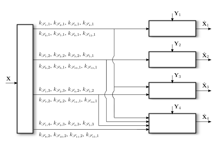
Choose the list vv as follows: 𝒮1={1,2,3,4}\mathscr{S}_{1}=\{1,2,3,4\}, 𝒮2={1,2,3}\mathscr{S}_{2}=\{1,2,3\}, 𝒮3={1,2,4}\mathscr{S}_{3}=\{1,2,4\}, 𝒮4={1,3,4}\mathscr{S}_{4}=\{1,3,4\}, 𝒮5={2,3,4}\mathscr{S}_{5}=\{2,3,4\}, 𝒮6={1,2}\mathscr{S}_{6}=\{1,2\}, 𝒮7={1,3}\mathscr{S}_{7}=\{1,3\}, 𝒮8={1,4}\mathscr{S}_{8}=\{1,4\}, 𝒮9={2,3}\mathscr{S}_{9}=\{2,3\}, 𝒮10={2,4}\mathscr{S}_{10}=\{2,4\}, 𝒮11={3,4}\mathscr{S}_{11}=\{3,4\}, 𝒮12={1}\mathscr{S}_{12}=\{1\}, 𝒮13={2}\mathscr{S}_{13}=\{2\}, 𝒮14={3}\mathscr{S}_{14}=\{3\} and 𝒮15={4}\mathscr{S}_{15}=\{4\}. Figure 6 shows the 33-layer nested codebook associated with the subset {1,2,3}\{1,2,3\}. In the first layer, there are 2n​R123,12^{nR_{123,1}} bins (labelled with the index k123,1k_{123,1}) each of which contain 2n⁡(R123′+R123,2+R123,3)2^{n(R^{\prime}_{123}+R_{123,2}+R_{123,3})} codewords. The set of codewords inside a particular layer one bin define the second layer of the codebook. Specifically, each layer one index k123,1∈[2n​R123,1]k_{123,1}\in[2^{nR_{123,1}}] identifies 2n​R123,22^{nR_{123,2}} layer two bins. These bins are labelled with the index k123,2k_{123,2}, and each bin contains 2n⁡(R123′+R123,3)2^{n(R^{\prime}_{123}+R_{123,3})} codewords. Similarly, each pair k123,1∈[2n​R123,1]k_{123,1}\in[2^{nR_{123,1}}] and k123,2∈[2n​R123,2]k_{123,2}\in[2^{nR_{123,2}}] identifies 2n​R123,32^{nR_{123,3}} layer three bins. There are 2n⁡(R123′)2^{n(R^{\prime}_{123})} codewords in each one of the layer three bins.


Fig. 6: 44-Decoders Example: Figure shows the nested bin structure for the codebook 𝒮2={1,2,3}\mathscr{S}_{2}=\{1,2,3\}.

A-B Encoding

Encoding proceeds sequentially over (2t−1)(2^{t}-1)-stages using ϵ\epsilon-letter typical-set encoding rules. For this purpose, choose 0<ϵ0<ϵ1<⋯<ϵ2t0<\epsilon_{0}<\epsilon_{1}<\cdots<\epsilon_{2^{t}} to be arbitrarily small real numbers. The encoder is given 𝐱∈𝒳n\mathbf{x}\in\mathscr{X}^{n}. At encoding stage jj it selects the codebook with label 𝒮j\mathscr{S}_{j} and looks for an index vector 𝐤𝒮j\mathbf{k}_{\mathscr{S}_{j}} where the corresponding codeword 𝐮𝒮j​(𝐤𝒮j)\mathbf{u}_{\mathscr{S}_{j}}(\mathbf{k}_{\mathscr{S}_{j}}) is ϵj\epsilon_{j}-letter typical with 𝐱\mathbf{x} and

𝐮𝒮j⊃\displaystyle\mathbf{u}_{\mathscr{S}_{j}}^{\supset} ≜{𝐮𝒮i(𝐤𝒮i):i<j,𝒮i⊃𝒮j}, and\displaystyle\triangleq\big\{\mathbf{u}_{\mathscr{S}_{i}}(\mathbf{k}_{\mathscr{S}_{i}}):i<j,\ \mathscr{S}_{i}\supset\mathscr{S}_{j}\big\},\text{ and}\ (44a)
𝐮𝒮j†\displaystyle\mathbf{u}^{\dagger}_{\mathscr{S}_{j}} ≜{𝐮𝒮i(𝐤𝒮i):i<j,𝒮i⊉𝒮j,∃𝒮i′,i′>j,𝒮i′∩𝒮j≠∅,𝒮i∩𝒮i′≠∅}.\displaystyle\triangleq\big\{\mathbf{u}_{\mathscr{S}_{i}}(\mathbf{k}_{\mathscr{S}_{i}}):i<j,\ \mathscr{S}_{i}\nsupseteq\mathscr{S}_{j},\ \exists\mathscr{S}_{i^{\prime}},\ i^{\prime}>j,\ \mathscr{S}_{i^{\prime}}\cap\mathscr{S}_{j}\neq\emptyset,\ \mathscr{S}_{i}\cap\mathscr{S}_{i^{\prime}}\neq\emptyset\big\}\ . (44b)

If successful88 8 If there are two-or-more such codewords, we assume that the encoder selects one codeword arbitrarily and sends the corresponding indices., the encoder sends the bin index k𝒮j,ik_{\mathscr{S}_{j},i} over channel 𝒮j​[i]\mathscr{S}_{j}[i] for every i=1,2,…,|𝒮j|i=1,2,\dots,|\mathscr{S}_{j}|. If unsuccessful, the encoder sends k𝒮j,i=1k_{\mathscr{S}_{j},i}=1 over each of these channels.

Note the correspondence between the sets 𝐮𝒮j⊃\mathbf{u}_{\mathscr{S}_{j}}^{\supset} and 𝐮𝒮j†\mathbf{u}^{\dagger}_{\mathscr{S}_{j}} and the sets of auxiliary random variables 𝒰𝒮j⊃\mathscr{U}_{\mathscr{S}_{j}}^{\supset} and 𝒰𝒮j†\mathscr{U}_{\mathscr{S}_{j}}^{{\dagger}}, respectively. Finally, note that when |𝒮j|≥3|\mathscr{S}_{j}|\geq 3, then 𝐮𝒮j⊃∪𝐮𝒮j†={𝐮𝒮i​(𝐤𝒮i):i<j}\mathbf{u}_{\mathscr{S}_{j}}^{\supset}\cup\mathbf{u}^{\dagger}_{\mathscr{S}_{j}}=\{\mathbf{u}_{\mathscr{S}_{i}}(\mathbf{k}_{\mathscr{S}_{i}}):i<j\}; that is, the encoder chooses 𝐮𝒮j​(𝐤𝒮j)\mathbf{u}_{\mathscr{S}_{j}}(\mathbf{k}_{\mathscr{S}_{j}}) to be jointly typical with every codeword it has previously selected. The situation is more complex when |𝒮j|≤2|\mathscr{S}_{j}|\leq 2.

Subset ​𝒮j𝐮𝒮j⊃,𝐮^𝒮j⊃𝐮𝒮j†𝐮^𝒮j,l‡𝒮1={1,2,3,4}∅∅∅𝒮2={1,2,3}{𝐮𝒮1}∅∅𝒮3={1,2,4}{𝐮𝒮1}{𝐮𝒮2}𝐮^𝒮3,1‡={𝐮𝒮2}𝐮^𝒮3,2‡={𝐮𝒮2}𝐮^𝒮3,4‡=∅𝒮4={1,3,4}{𝐮𝒮1}{𝐮𝒮2,𝐮𝒮3}𝐮^𝒮4,1‡={𝐮𝒮2,𝐮𝒮3}𝐮^𝒮4,3‡={𝐮𝒮2}𝐮^𝒮4,4‡={𝐮𝒮3}𝒮5={2,3,4}{𝐮𝒮1}{𝐮𝒮2,𝐮𝒮3,𝐮𝒮4}𝐮^𝒮5,2‡={𝐮𝒮2,𝐮𝒮3}𝐮^𝒮5,3‡={𝐮𝒮2,𝐮𝒮4}𝐮^𝒮5,4‡={𝐮𝒮3,𝐮𝒮4}𝒮6={1,2}{𝐮𝒮1,𝐮𝒮2,𝐮𝒮3}{𝐮𝒮4,𝐮𝒮5}𝐮^𝒮6,1‡={𝐮𝒮4}𝐮^𝒮6,2‡={𝐮𝒮5}𝒮7={1,3}{𝐮𝒮1,𝐮𝒮2,𝐮𝒮4}{𝐮𝒮3,𝐮𝒮5,𝐮𝒮6}𝐮^𝒮7,1‡={𝐮𝒮3,𝐮𝒮6}𝐮^𝒮7,3‡={𝐮𝒮5}𝒮8={1,4}{𝐮𝒮1,𝐮𝒮3,𝐮𝒮4}{𝐮𝒮2,𝐮𝒮5,𝐮𝒮6,𝐮𝒮7}𝐮^𝒮8,1‡={𝐮𝒮2,𝐮𝒮6,𝐮𝒮7}𝐮^𝒮8,4‡={𝐮𝒮5}𝒮9={2,3}{𝐮𝒮1,𝐮𝒮2,𝐮𝒮5}{𝐮𝒮3,𝐮𝒮4,𝐮𝒮6,𝐮𝒮7,𝐮𝒮8}𝐮^𝒮9,2‡={𝐮𝒮3,𝐮𝒮6}𝐮^𝒮9,3‡={𝐮𝒮4,𝐮𝒮7}𝒮10={2,4}{𝐮𝒮1,𝐮𝒮3,𝐮𝒮5}{𝐮𝒮2,𝐮𝒮4,𝐮𝒮6,𝐮𝒮7,𝐮𝒮8,𝐮𝒮9}𝐮^𝒮10,2‡={𝐮𝒮2,𝐮𝒮6,𝐮𝒮9}𝐮^𝒮10,4‡={𝐮𝒮4,𝐮𝒮8}𝒮11={3,4}{𝐮𝒮1,𝐮𝒮4,𝐮𝒮5}{𝐮‡𝒮2,𝐮𝒮3,𝐮𝒮7,𝐮𝒮8,𝐮‡𝒮9,𝐮𝒮10}𝐮^𝒮11,3‡={𝐮𝒮2,𝐮𝒮7,𝐮𝒮9}𝐮^𝒮11,4‡={𝐮𝒮3,𝐮𝒮8,𝐮𝒮10}𝒮12={1}{𝐮𝒮1,𝐮𝒮2,𝐮𝒮3,𝐮𝒮4,𝐮𝒮6,𝐮𝒮7,𝐮𝒮8}∅∅𝒮13={2}{𝐮𝒮1,𝐮𝒮2,𝐮𝒮3,𝐮𝒮5,𝐮𝒮6,𝐮𝒮9,𝐮𝒮10}∅∅𝒮14={3}{𝐮𝒮1,𝐮𝒮2,𝐮𝒮4,𝐮𝒮5,𝐮𝒮7,𝐮𝒮9,𝐮𝒮11}∅∅𝒮15={4}{𝐮𝒮1,𝐮𝒮3,𝐮𝒮4,𝐮𝒮5,𝐮𝒮8,𝐮𝒮10,𝐮𝒮11}∅∅\begin{array}[]{|c|c|c|c|}\hline\cr\text{Subset }\mathscr{S}_{j}&\mathbf{u}^{\supset}_{\mathscr{S}_{j}},\hat{\mathbf{u}}^{\supset}_{\mathscr{S}_{j}}&\mathbf{u}^{{\dagger}}_{\mathscr{S}_{j}}&\hat{\mathbf{u}}^{{\ddagger}}_{\mathscr{S}_{j},l}\\ \hline\cr\mathscr{S}_{1}=\{1,2,3,4\}&\emptyset&\emptyset&\emptyset\\ \hline\cr\mathscr{S}_{2}=\{1,2,3\}&\{\mathbf{u}_{\mathscr{S}_{1}}\}&\emptyset&\emptyset\\ \hline\cr\mathscr{S}_{3}=\{1,2,4\}&\{\mathbf{u}_{\mathscr{S}_{1}}\}&\{\mathbf{u}_{\mathscr{S}_{2}}\}&\begin{array}[]{c}\hat{\mathbf{u}}^{\ddagger}_{\mathscr{S}_{3},1}=\{\mathbf{u}_{\mathscr{S}_{2}}\}\\ \hat{\mathbf{u}}^{\ddagger}_{\mathscr{S}_{3},2}=\{\mathbf{u}_{\mathscr{S}_{2}}\}\\ \hat{\mathbf{u}}^{\ddagger}_{\mathscr{S}_{3},4}=\emptyset\end{array}\\ \hline\cr\mathscr{S}_{4}=\{1,3,4\}&\{\mathbf{u}_{\mathscr{S}_{1}}\}&\{\mathbf{u}_{\mathscr{S}_{2}},\mathbf{u}_{\mathscr{S}_{3}}\}&\begin{array}[]{c}\hat{\mathbf{u}}^{\ddagger}_{\mathscr{S}_{4},1}=\{\mathbf{u}_{\mathscr{S}_{2}},\mathbf{u}_{\mathscr{S}_{3}}\}\\ \hat{\mathbf{u}}^{\ddagger}_{\mathscr{S}_{4},3}=\{\mathbf{u}_{\mathscr{S}_{2}}\}\\ \hat{\mathbf{u}}^{\ddagger}_{\mathscr{S}_{4},4}=\{\mathbf{u}_{\mathscr{S}_{3}}\}\end{array}\\ \hline\cr\mathscr{S}_{5}=\{2,3,4\}&\{\mathbf{u}_{\mathscr{S}_{1}}\}&\{\mathbf{u}_{\mathscr{S}_{2}},\mathbf{u}_{\mathscr{S}_{3}},\mathbf{u}_{\mathscr{S}_{4}}\}&\begin{array}[]{c}\hat{\mathbf{u}}^{\ddagger}_{\mathscr{S}_{5},2}=\{\mathbf{u}_{\mathscr{S}_{2}},\mathbf{u}_{\mathscr{S}_{3}}\}\\ \hat{\mathbf{u}}^{\ddagger}_{\mathscr{S}_{5},3}=\{\mathbf{u}_{\mathscr{S}_{2}},\mathbf{u}_{\mathscr{S}_{4}}\}\\ \hat{\mathbf{u}}^{\ddagger}_{\mathscr{S}_{5},4}=\{\mathbf{u}_{\mathscr{S}_{3}},\mathbf{u}_{\mathscr{S}_{4}}\}\end{array}\\ \hline\cr\mathscr{S}_{6}=\{1,2\}&\{\mathbf{u}_{\mathscr{S}_{1}},\mathbf{u}_{\mathscr{S}_{2}},\mathbf{u}_{\mathscr{S}_{3}}\}&\{\mathbf{u}_{\mathscr{S}_{4}},\mathbf{u}_{\mathscr{S}_{5}}\}&\begin{array}[]{c}\hat{\mathbf{u}}^{\ddagger}_{\mathscr{S}_{6},1}=\{\mathbf{u}_{\mathscr{S}_{4}}\}\\ \hat{\mathbf{u}}^{\ddagger}_{\mathscr{S}_{6},2}=\{\mathbf{u}_{\mathscr{S}_{5}}\}\end{array}\\ \hline\cr\mathscr{S}_{7}=\{1,3\}&\{\mathbf{u}_{\mathscr{S}_{1}},\mathbf{u}_{\mathscr{S}_{2}},\mathbf{u}_{\mathscr{S}_{4}}\}&\{\mathbf{u}_{\mathscr{S}_{3}},\mathbf{u}_{\mathscr{S}_{5}},\mathbf{u}_{\mathscr{S}_{6}}\}&\begin{array}[]{c}\hat{\mathbf{u}}^{\ddagger}_{\mathscr{S}_{7},1}=\{\mathbf{u}_{\mathscr{S}_{3}},\mathbf{u}_{\mathscr{S}_{6}}\}\\ \hat{\mathbf{u}}^{\ddagger}_{\mathscr{S}_{7},3}=\{\mathbf{u}_{\mathscr{S}_{5}}\}\end{array}\\ \hline\cr\mathscr{S}_{8}=\{1,4\}&\{\mathbf{u}_{\mathscr{S}_{1}},\mathbf{u}_{\mathscr{S}_{3}},\mathbf{u}_{\mathscr{S}_{4}}\}&\{\mathbf{u}_{\mathscr{S}_{2}},\mathbf{u}_{\mathscr{S}_{5}},\mathbf{u}_{\mathscr{S}_{6}},\mathbf{u}_{\mathscr{S}_{7}}\}&\begin{array}[]{c}\hat{\mathbf{u}}^{\ddagger}_{\mathscr{S}_{8},1}=\{\mathbf{u}_{\mathscr{S}_{2}},\mathbf{u}_{\mathscr{S}_{6}},\mathbf{u}_{\mathscr{S}_{7}}\}\\ \hat{\mathbf{u}}^{\ddagger}_{\mathscr{S}_{8},4}=\{\mathbf{u}_{\mathscr{S}_{5}}\}\end{array}\\ \hline\cr\mathscr{S}_{9}=\{2,3\}&\{\mathbf{u}_{\mathscr{S}_{1}},\mathbf{u}_{\mathscr{S}_{2}},\mathbf{u}_{\mathscr{S}_{5}}\}&\begin{array}[]{c}\{\mathbf{u}_{\mathscr{S}_{3}},\mathbf{u}_{\mathscr{S}_{4}},\mathbf{u}_{\mathscr{S}_{6}},\mathbf{u}_{\mathscr{S}_{7}},\\ \mathbf{u}_{\mathscr{S}_{8}}\}\end{array}&\begin{array}[]{c}\hat{\mathbf{u}}^{\ddagger}_{\mathscr{S}_{9},2}=\{\mathbf{u}_{\mathscr{S}_{3}},\mathbf{u}_{\mathscr{S}_{6}}\}\\ \hat{\mathbf{u}}^{\ddagger}_{\mathscr{S}_{9},3}=\{\mathbf{u}_{\mathscr{S}_{4}},\mathbf{u}_{\mathscr{S}_{7}}\}\end{array}\\ \hline\cr\mathscr{S}_{10}=\{2,4\}&\{\mathbf{u}_{\mathscr{S}_{1}},\mathbf{u}_{\mathscr{S}_{3}},\mathbf{u}_{\mathscr{S}_{5}}\}&\begin{array}[]{c}\{\mathbf{u}_{\mathscr{S}_{2}},\mathbf{u}_{\mathscr{S}_{4}},\mathbf{u}_{\mathscr{S}_{6}},\mathbf{u}_{\mathscr{S}_{7}},\\ \mathbf{u}_{\mathscr{S}_{8}},\mathbf{u}_{\mathscr{S}_{9}}\}\end{array}&\begin{array}[]{c}\hat{\mathbf{u}}^{\ddagger}_{\mathscr{S}_{10},2}=\{\mathbf{u}_{\mathscr{S}_{2}},\mathbf{u}_{\mathscr{S}_{6}},\mathbf{u}_{\mathscr{S}_{9}}\}\\ \hat{\mathbf{u}}^{\ddagger}_{\mathscr{S}_{10},4}=\{\mathbf{u}_{\mathscr{S}_{4}},\mathbf{u}_{\mathscr{S}_{8}}\}\end{array}\\ \hline\cr\mathscr{S}_{11}=\{3,4\}&\{\mathbf{u}_{\mathscr{S}_{1}},\mathbf{u}_{\mathscr{S}_{4}},\mathbf{u}_{\mathscr{S}_{5}}\}&\begin{array}[]{c}\{\mathbf{u}^{\ddagger}_{\mathscr{S}_{2}},\mathbf{u}_{\mathscr{S}_{3}},\mathbf{u}_{\mathscr{S}_{7}},\mathbf{u}_{\mathscr{S}_{8}},\\ \mathbf{u}^{\ddagger}_{\mathscr{S}_{9}},\mathbf{u}_{\mathscr{S}_{10}}\}\end{array}&\begin{array}[]{c}\hat{\mathbf{u}}^{\ddagger}_{\mathscr{S}_{11},3}=\{\mathbf{u}_{\mathscr{S}_{2}},\mathbf{u}_{\mathscr{S}_{7}},\mathbf{u}_{\mathscr{S}_{9}}\}\\ \hat{\mathbf{u}}^{\ddagger}_{\mathscr{S}_{11},4}=\{\mathbf{u}_{\mathscr{S}_{3}},\mathbf{u}_{\mathscr{S}_{8}},\mathbf{u}_{\mathscr{S}_{10}}\}\end{array}\\ \hline\cr\mathscr{S}_{12}=\{1\}&\begin{array}[]{c}\{\mathbf{u}_{\mathscr{S}_{1}},\mathbf{u}_{\mathscr{S}_{2}},\mathbf{u}_{\mathscr{S}_{3}},\mathbf{u}_{\mathscr{S}_{4}},\\ \mathbf{u}_{\mathscr{S}_{6}},\mathbf{u}_{\mathscr{S}_{7}},\mathbf{u}_{\mathscr{S}_{8}}\}\end{array}&\emptyset&\emptyset\\ \hline\cr\mathscr{S}_{13}=\{2\}&\begin{array}[]{c}\{\mathbf{u}_{\mathscr{S}_{1}},\mathbf{u}_{\mathscr{S}_{2}},\mathbf{u}_{\mathscr{S}_{3}},\mathbf{u}_{\mathscr{S}_{5}},\\ \mathbf{u}_{\mathscr{S}_{6}},\mathbf{u}_{\mathscr{S}_{9}},\mathbf{u}_{\mathscr{S}_{10}}\}\end{array}&\emptyset&\emptyset\\ \hline\cr\mathscr{S}_{14}=\{3\}&\begin{array}[]{c}\{\mathbf{u}_{\mathscr{S}_{1}},\mathbf{u}_{\mathscr{S}_{2}},\mathbf{u}_{\mathscr{S}_{4}},\mathbf{u}_{\mathscr{S}_{5}},\\ \mathbf{u}_{\mathscr{S}_{7}},\mathbf{u}_{\mathscr{S}_{9}},\mathbf{u}_{\mathscr{S}_{11}}\}\end{array}&\emptyset&\emptyset\\ \hline\cr\mathscr{S}_{15}=\{4\}&\begin{array}[]{c}\{\mathbf{u}_{\mathscr{S}_{1}},\mathbf{u}_{\mathscr{S}_{3}},\mathbf{u}_{\mathscr{S}_{4}},\mathbf{u}_{\mathscr{S}_{5}},\\ \mathbf{u}_{\mathscr{S}_{8}},\mathbf{u}_{\mathscr{S}_{10}},\mathbf{u}_{\mathscr{S}_{11}}\}\end{array}&\emptyset&\emptyset\\ \hline\cr\end{array}
TABLE I: The table lists the fifteen encoding sets 𝐮𝒮j⊃\mathbf{u}^{\supset}_{\mathscr{S}_{j}} and 𝐮𝒮j†\mathbf{u}^{{\dagger}}_{\mathscr{S}_{j}} as well as the decoding sets 𝐮^𝒮j⊃\hat{\mathbf{u}}^{\supset}_{\mathscr{S}_{j}} and 𝐮^𝒮j‡\hat{\mathbf{u}}^{{\ddagger}}_{\mathscr{S}_{j}} for the four decoder example.
Example 5 (44-Decoders Encoding)

Table I lists the fifteen encoding sets 𝐮𝒮j⊃\mathbf{u}^{\supset}_{\mathscr{S}_{j}} and 𝐮𝒮j†\mathbf{u}^{{\dagger}}_{\mathscr{S}_{j}} and Figure 7 depicts the index to channel assignments for the four decoder example. In stage 11, the encoder considers subset 𝒮1\mathscr{S}_{1} and looks for an index vector 𝐤𝒮1\mathbf{k}_{\mathscr{S}_{1}} such that the corresponding codeword 𝐮𝒮1​(𝐤𝒮1)\mathbf{u}_{\mathscr{S}_{1}}(\mathbf{k}_{\mathscr{S}_{1}}) is jointly typical with 𝐱\mathbf{x}. (The sets 𝐮𝒮1⊃\mathbf{u}^{\supset}_{\mathscr{S}_{1}} and 𝐮𝒮1†\mathbf{u}^{{\dagger}}_{\mathscr{S}_{1}} are empty – see Table I.) The resulting indices k𝒮1,1k_{\mathscr{S}_{1},1}, k𝒮1,2k_{\mathscr{S}_{1},2}, k𝒮1,3k_{\mathscr{S}_{1},3} and k𝒮1,4k_{\mathscr{S}_{1},4} are sent over channels 11, 22, 33 and 44, respectively. In the eleventh encoding stage, takes the codebook for 𝒮11={3,4}\mathscr{S}_{11}=\{3,4\} and looks for a index vector 𝐤𝒮11=(k𝒮11,1,k𝒮11,2,k𝒮11′)\mathbf{k}_{\mathscr{S}_{11}}=(k_{\mathscr{S}_{11},1},k_{\mathscr{S}_{11},2},k^{\prime}_{\mathscr{S}_{11}}) such that the corresponding codeword 𝐮𝒮11​(𝐤𝒮11)\mathbf{u}_{\mathscr{S}_{11}}(\mathbf{k}_{\mathscr{S}_{11}}) is jointly typical with 𝐱\mathbf{x}, 𝐮𝒮1​(𝐤𝒮1)\mathbf{u}_{\mathscr{S}_{1}}(\mathbf{k}_{\mathscr{S}_{1}}) through to 𝐮𝒮5​(𝐤𝒮5)\mathbf{u}_{\mathscr{S}_{5}}(\mathbf{k}_{\mathscr{S}_{5}}) and 𝐮𝒮7​(𝐤𝒮7)\mathbf{u}_{\mathscr{S}_{7}}(\mathbf{k}_{\mathscr{S}_{7}}) through to 𝐮𝒮10​(𝐤𝒮10)\mathbf{u}_{\mathscr{S}_{10}}(\mathbf{k}_{\mathscr{S}_{10}}). (Note, that this codeword need not be jointly typical with 𝐮𝒮6​(𝐤𝒮6)\mathbf{u}_{\mathscr{S}_{6}}(\mathbf{k}_{\mathscr{S}_{6}}).) The resulting indices k𝒮11,1k_{\mathscr{S}_{11},1}, k𝒮11,2k_{\mathscr{S}_{11},2} are sent over channels 33 and 44, respectively.

Refer to caption

Fig. 7: 44-Decoders Example: Assignment of bin indices to channels. Subsets are 𝒮1={1,2,3,4}\mathscr{S}_{1}=\{1,2,3,4\}, 𝒮2={1,2,3}\mathscr{S}_{2}=\{1,2,3\}, 𝒮3={1,2,4}\mathscr{S}_{3}=\{1,2,4\}, 𝒮4={1,3,4}\mathscr{S}_{4}=\{1,3,4\}, 𝒮5={2,3,4}\mathscr{S}_{5}=\{2,3,4\}, 𝒮6={1,2}\mathscr{S}_{6}=\{1,2\}, 𝒮7={1,3}\mathscr{S}_{7}=\{1,3\}, 𝒮8={1,4}\mathscr{S}_{8}=\{1,4\}, 𝒮9={2,3}\mathscr{S}_{9}=\{2,3\}, 𝒮10={2,4}\mathscr{S}_{10}=\{2,4\}, 𝒮11={3,4}\mathscr{S}_{11}=\{3,4\}, 𝒮12={1}\mathscr{S}_{12}=\{1\}, 𝒮13={2}\mathscr{S}_{13}=\{2\}, 𝒮14={3}\mathscr{S}_{14}=\{3\} and 𝒮15={4}\mathscr{S}_{15}=\{4\}. Bin index k𝒮j,ik_{\mathscr{S}_{j},i} is sent over channel 𝒮j​[i]\mathscr{S}_{j}[i].

A-C Decoding

Consider decoder ll. Like the encoding procedure, decoder ll forms its reconstruction 𝐗^l\hat{\mathbf{X}}_{l} of 𝐗\mathbf{X} using (2t−1)(2^{t}-1)-decoding stages. Recall, this decoder recovers every bin index transmitted on channels 11 through ll; it does not have access to any index transmitted on channels l+1l+1 through tt.

In stage jj decoder ll considers subset 𝒮j\mathscr{S}_{j}. If l∉𝒮jl\notin\mathscr{S}_{j}, then it does nothing and moves to decoding stage j+1j+1. If l∈𝒮jl\in\mathscr{S}_{j}, then the decoder forms a reconstruction 𝐮𝒮j​(𝐤^𝒮j)\mathbf{u}_{\mathscr{S}_{j}}(\hat{\mathbf{k}}_{\mathscr{S}_{j}}) of the codeword 𝐮𝒮j​(𝐤𝒮j)\mathbf{u}_{\mathscr{S}_{j}}(\mathbf{k}_{\mathscr{S}_{j}}), which was selected by the encoder, using the following procedure. Note, decoder ll will have reconstructed the following codewords in decoding stages 11 through j−1j-1:

𝐮^𝒮j⊃≜{𝐮𝒮i(𝐤^𝒮i):i<j,𝒮i⊃𝒮j}, and\hat{\mathbf{u}}_{\mathscr{S}_{j}}^{\supset}\triangleq\big\{\mathbf{u}_{\mathscr{S}_{i}}(\hat{\mathbf{k}}_{\mathscr{S}_{i}}):i<j,\ \mathscr{S}_{i}\supset\mathscr{S}_{j}\big\},\text{ and} (45a)
𝐮^𝒮j,l‡≜{𝐮𝒮i(𝐤^𝒮i):i<j,𝒮i∋l,𝒮i⊉𝒮j}.\hat{\mathbf{u}}^{\ddagger}_{\mathscr{S}_{j},l}\triangleq\big\{\mathbf{u}_{\mathscr{S}_{i}}(\hat{\mathbf{k}}_{\mathscr{S}_{i}}):i<j,\ \mathscr{S}_{i}\ni l,\ \mathscr{S}_{i}\nsupseteq\mathscr{S}_{j}\big\}\ . (45b)

Note the correspondence between the decoding sets in (45) and the sets of auxiliary random variables 𝒜𝒮j⊃\mathscr{A}^{\supset}_{\mathscr{S}_{j}} and 𝒜𝒮j,l‡\mathscr{A}^{\ddagger}_{\mathscr{S}_{j},l}.

To form its reconstruction 𝐮𝒮j​(𝐤^𝒮j)\mathbf{u}_{\mathscr{S}_{j}}(\hat{\mathbf{k}}_{\mathscr{S}_{j}}), decoder ll takes the bin indices

{k𝒮j,i;i=1,2,…,|[l]∩𝒮j|}\left\{k_{\mathscr{S}_{j},i};\ i=1,2,\ldots,|[l]\cap\mathscr{S}_{j}|\right\}

from channels 11 through ll. It then looks for an index vector 𝐤~𝒮j\tilde{\mathbf{k}}_{\mathscr{S}_{j}}, with k~𝒮j,i=k𝒮j,i\tilde{k}_{\mathscr{S}_{j},i}=k_{\mathscr{S}_{j},i} for all i=1,2,…,|[l]∩𝒮j|i=1,2,\ldots,|[l]\cap\mathscr{S}_{j}|, such that the corresponding codeword 𝐮⁡(𝐤~𝒮j)\mathbf{u}(\tilde{\mathbf{k}}_{\mathscr{S}_{j}}) is ϵj+1\epsilon_{j+1}-letter typical with 𝐲l\mathbf{y}_{l} as well as the codewords in (45) that were decoded in the first (j−1)(j-1)-stages:

(𝐮^𝒮j⊃,𝐮^𝒮j,l‡,𝐮𝒮j​(𝐤~𝒮j),𝐲l)∈Tϵj+1(n)​(p).\left(\hat{\mathbf{u}}_{\mathscr{S}_{j}}^{\supset},\ \hat{\mathbf{u}}^{\ddagger}_{\mathscr{S}_{j},l},\ \mathbf{u}_{\mathscr{S}_{j}}(\tilde{\mathbf{k}}_{\mathscr{S}_{j}}),\mathbf{y}_{l}\right)\in T_{\epsilon_{j+1}}^{(n)}(p). (46)

Note that there are

exp2⁡[n⁡(R𝒮j′+∑i=|[l]∩𝒮j|+1|𝒮j|R𝒮j,i)]\exp_{2}\left[{n\left(R^{\prime}_{\mathscr{S}_{j}}+\sum_{i=|[l]\cap\mathscr{S}_{j}|+1}^{|\mathscr{S}_{j}|}R_{\mathscr{S}_{j},i}\right)}\right]

codewords in the bin specified by the indices {k𝒮j,i:i=1,2,…,|[l]∩𝒮j|}\{k_{\mathscr{S}_{j},i}:i=1,2,\ldots,|[l]\cap\mathscr{S}_{j}|\}. If one or more of these codewords satisfy this typicality condition, then decoder ll selects one arbitrarily and sets 𝐤^𝒮j=𝐤~𝒮j\hat{\mathbf{k}}_{\mathscr{S}_{j}}=\tilde{\mathbf{k}}_{\mathscr{S}_{j}}. If there is no such codeword, it sets each of the unknown indices equal to 11.

Example 6 (44-Decoders Decoding)

Consider the second decoder (l=2)(l=2). In stage one, take k𝒮1,1k_{\mathscr{S}_{1},1} (from channel 11) and k𝒮1,2k_{\mathscr{S}_{1},2} (from channel 22) and look for a vector 𝐤~𝒮1\tilde{\mathbf{k}}_{\mathscr{S}_{1}} == (k𝒮1,1𝐶𝐿𝑂𝑆𝐸(k_{\mathscr{S}_{1},1}, k𝒮1,2k_{\mathscr{S}_{1},2}, 𝑂𝑃𝐸𝑁k~𝒮1,3,k~𝒮1′)\tilde{k}_{\mathscr{S}_{1},3},\tilde{k}^{\prime}_{\mathscr{S}_{1}}) such that the corresponding codeword 𝐮𝒮1​(𝐤~𝒮1)\mathbf{u}_{\mathscr{S}_{1}}(\tilde{\mathbf{k}}_{\mathscr{S}_{1}}) is typical with 𝐲2\mathbf{y}_{2}. Similarly, in stage nine take k𝒮9,1k_{\mathscr{S}_{9},1} (from channel 22) and look for 𝐤~𝒮9=(k𝒮9,1,k~𝒮9,2,k~𝒮9′)\tilde{\mathbf{k}}_{\mathscr{S}_{9}}=(k_{\mathscr{S}_{9},1},\tilde{k}_{\mathscr{S}_{9},2},\tilde{k}^{\prime}_{\mathscr{S}_{9}}) such that the corresponding codeword 𝐮𝒮9​(𝐤~𝒮9)\mathbf{u}_{\mathscr{S}_{9}}(\tilde{\mathbf{k}}_{\mathscr{S}_{9}}) is jointly typical with 𝐲2\mathbf{y}_{2} and 𝐮𝒮1​(𝐤^𝒮1)\mathbf{u}_{\mathscr{S}_{1}}(\hat{\mathbf{k}}_{\mathscr{S}_{1}}), 𝐮𝒮2​(𝐤^𝒮2)\mathbf{u}_{\mathscr{S}_{2}}(\hat{\mathbf{k}}_{\mathscr{S}_{2}}), 𝐮𝒮3​(𝐤^𝒮3)\mathbf{u}_{\mathscr{S}_{3}}(\hat{\mathbf{k}}_{\mathscr{S}_{3}}), 𝐮𝒮5​(𝐤^𝒮5)\mathbf{u}_{\mathscr{S}_{5}}(\hat{\mathbf{k}}_{\mathscr{S}_{5}}) and 𝐮𝒮6​(𝐤^𝒮6)\mathbf{u}_{\mathscr{S}_{6}}(\hat{\mathbf{k}}_{\mathscr{S}_{6}}), which were decoded during stages one through six. Finally, in stage thirteen take k𝒮13,1k_{\mathscr{S}_{13},1} (from channel 22) and look for 𝐤~𝒮13=(k𝒮12,1,k~𝒮13′)\tilde{\mathbf{k}}_{\mathscr{S}_{13}}=(k_{\mathscr{S}_{12},1},\tilde{k}^{\prime}_{\mathscr{S}_{13}}) such that the corresponding codeword 𝐮𝒮13​(𝐤~𝒮6)\mathbf{u}_{\mathscr{S}_{13}}(\tilde{\mathbf{k}}_{\mathscr{S}_{6}}) is jointly typical with 𝐲2\mathbf{y}_{2} and 𝐮𝒮1​(𝐤^𝒮1)\mathbf{u}_{\mathscr{S}_{1}}(\hat{\mathbf{k}}_{\mathscr{S}_{1}}), 𝐮𝒮2​(𝐤^𝒮2)\mathbf{u}_{\mathscr{S}_{2}}(\hat{\mathbf{k}}_{\mathscr{S}_{2}}), 𝐮𝒮3​(𝐤^𝒮3)\mathbf{u}_{\mathscr{S}_{3}}(\hat{\mathbf{k}}_{\mathscr{S}_{3}}), 𝐮𝒮5​(𝐤^𝒮5)\mathbf{u}_{\mathscr{S}_{5}}(\hat{\mathbf{k}}_{\mathscr{S}_{5}}), 𝐮𝒮6​(𝐤^𝒮6)\mathbf{u}_{\mathscr{S}_{6}}(\hat{\mathbf{k}}_{\mathscr{S}_{6}}), 𝐮𝒮9​(𝐤^𝒮9)\mathbf{u}_{\mathscr{S}_{9}}(\hat{\mathbf{k}}_{\mathscr{S}_{9}}) and 𝐮𝒮10​(𝐤^𝒮10)\mathbf{u}_{\mathscr{S}_{10}}(\hat{\mathbf{k}}_{\mathscr{S}_{10}}), which were decoded during stages one through ten.

A-D Error Analysis: Encoding

The coding scheme is based on ϵ\epsilon-letter typical set encoding and decoding techniques. As such, the distortion criteria at each decoder will not be satisfied when (𝐱,𝐲1,𝐲2,…,𝐲t)∉Tϵ0(n)​(p)\left(\mathbf{x},\mathbf{y}_{1},\mathbf{y}_{2},\dots,\mathbf{y}_{t}\right)\notin T^{(n)}_{\epsilon_{0}}(p). We denote this event by E1E_{1}. From Lemma 2, the probability of this event may be bound by

Pr⁡[E1]≤δ1​(n,ϵ0,μ⁡(p)),\Pr\left[E_{1}\right]\leq\delta_{1}\left(n,\epsilon_{0},\mu(p)\right)\ ,

where δ1​(n,ϵ0,μ⁡(p))→0\delta_{1}\left(n,\epsilon_{0},\mu(p)\right){\rightarrow}0 as n→∞n\rightarrow\infty.

Assume E1E_{1} does not occur. Let E2,𝒮jE_{2,\mathscr{S}_{j}} denote the event that the encoder fails to find an ϵj\epsilon_{j}-letter typical codeword during stage jj of encoding procedure given that it found an ϵi\epsilon_{i}-letter typical codeword for every stage i∈[j−1]i\in[j-1]. From Lemma 3 and the inequality (1−x)t≤e−t​x(1-x)^{t}\leq e^{-tx} we have

Pr⁡[E2,𝒮j]\displaystyle\Pr\left[E_{2,\mathscr{S}_{j}}\right] =[1−Pr[(𝐮𝒮j⊃,𝐮𝒮j†,𝐔𝒮j(𝐤𝒮j),𝐱)∈Tϵj+1(n)(p)]]2n⁡(R𝒮j′+∑i=1|Sj|R𝒮j,i)\displaystyle=\Bigg[1-\text{Pr}\Big[\big(\mathbf{u}^{\supset}_{\mathscr{S}_{j}},\mathbf{u}^{{\dagger}}_{\mathscr{S}_{j}},\mathbf{U}_{\mathscr{S}_{j}}(\mathbf{k}_{\mathscr{S}_{j}}),\mathbf{x}\big)\in T^{(n)}_{\epsilon_{j+1}}(p)\Big]\Bigg]^{2^{n\left(R^{\prime}_{\mathscr{S}_{j}}+\sum_{i=1}^{|S_{j}|}R_{\mathscr{S}_{j},i}\right)}}
≤exp(−(1−δ2)2n⁡(R𝒮j′+∑i=1|Sj|R𝒮j,i)⋅2−n⁡(I⁡(𝒜𝒮j⊃,𝒜𝒮j†,X,U𝒮j)+2​ϵj​H​(U𝒮j)))\displaystyle\leq\exp\Bigg(-\big(1-\delta_{2}\big)2^{n\left(R^{\prime}_{\mathscr{S}_{j}}+\sum_{i=1}^{|S_{j}|}R_{\mathscr{S}_{j},i}\right)}\cdot 2^{-n\Big(I\left(\mathscr{A}^{\supset}_{\mathscr{S}_{j}},\mathscr{A}^{\dagger}_{\mathscr{S}_{j}},X;U_{\mathscr{S}_{j}}\right)+2\epsilon_{j}H\left(U_{\mathscr{S}_{j}}\right)\Big)}\Bigg) (47)

where we have written the function δ2​(n,ϵj−1,ϵj,μ⁡(p))\delta_{2}\left(n,\epsilon_{j-1},\epsilon_{j},\mu(p)\right) as δ2\delta_{2} for compact representation.

Let E2E_{2} denote the event where a typical codeword cannot be found at any one of the encoding stages. By the union bound we get the following upper bound for Pr​[E2]\text{Pr}[E_{2}]:

Pr[E2]≤∑j=12t−1exp[\displaystyle\Pr\left[E_{2}\right]\leq\sum_{j=1}^{2^{t}-1}\exp\Bigg[ −(1−δ2)2n⁡(R𝒮j′+∑i=1|Sj|R𝒮j,i)⋅2−n⁡[I⁡(𝒜𝒮j⊃,𝒜𝒮j†,X,U𝒮j)+2​ϵj​H​(U𝒮j)]].\displaystyle-\big(1-\delta_{2}\big)2^{n\left(R^{\prime}_{\mathscr{S}_{j}}+\sum_{i=1}^{|S_{j}|}R_{\mathscr{S}_{j},i}\right)}\cdot 2^{-n\Big[I\left(\mathscr{A}^{\supset}_{\mathscr{S}_{j}},\mathscr{A}^{\dagger}_{\mathscr{S}_{j}},X;U_{\mathscr{S}_{j}}\right)+2\epsilon_{j}H\left(U_{\mathscr{S}_{j}}\right)\Big]}\Bigg]\ .

Finally, note that if

R𝒮j′+∑i=1|𝒮j|R𝒮j,i>I⁡(𝒜𝒮j⊃,𝒜𝒮j†,X,U𝒮j)+2​ϵj​H​(U𝒮j)R^{\prime}_{\mathscr{S}_{j}}+\sum_{i=1}^{|\mathscr{S}_{j}|}R_{\mathscr{S}_{j},i}>I\left(\mathscr{A}^{\supset}_{\mathscr{S}_{j}},\mathscr{A}^{\dagger}_{\mathscr{S}_{j}},X;U_{\mathscr{S}_{j}}\right)+2\epsilon_{j}H\left(U_{\mathscr{S}_{j}}\right) (48)

for every j=1,2,…,2t−1j=1,2,\ldots,2^{t}-1, then Pr⁡[E2]→0\Pr[E_{2}]\rightarrow 0 as n→∞n\rightarrow\infty.

A-E Error Analysis: Decoding

Assume E1E_{1} and E2E_{2} do not occur. Consider decoder ll and a non-trivial decoding stage jj where 𝒮j∋l\mathscr{S}_{j}\ni l. Let Dl,𝒮jD_{l,\mathscr{S}_{j}} be the event that it cannot find a unique codeword that satisfies the typicality condition (46) given that at every stage i<ji<j (where 𝒮i∋l\mathscr{S}_{i}\ni l) it found a unique codeword 𝐮⁡(𝐤^𝒮i)\mathbf{u}(\hat{\mathbf{k}}_{\mathscr{S}_{i}}) satisfying this typicality condition.

By the Markov lemma (Lemma 4), the probability that the codewords 𝐮^𝒮j​(𝐤𝒮j)\hat{\mathbf{u}}_{\mathscr{S}_{j}}(\mathbf{k}_{\mathscr{S}_{j}}), 𝐮^𝒮j⊃\hat{\mathbf{u}}^{\supset}_{\mathscr{S}_{j}}, 𝐮𝒮j,l‡\mathbf{u}^{{\ddagger}}_{\mathscr{S}_{j},l} are not jointly typical with 𝐲l\mathbf{y}_{l} is small for large nn:

Pr[𝐘l∉Tϵj+1(n)(p∣𝐮^𝒮j⊃,𝐮^𝒮j,l‡𝐮𝒮j(𝐤𝒮j),𝐱)]≤δ2(n,ϵj,ϵj+1,μ(p)).\Pr\left[\mathbf{Y}_{l}\notin T^{(n)}_{\epsilon_{j+1}}\left(p\mid\hat{\mathbf{u}}^{\supset}_{\mathscr{S}_{j}},\hat{\mathbf{u}}^{{\ddagger}}_{\mathscr{S}_{j},l}\mathbf{u}_{\mathscr{S}_{j}}(\mathbf{k}_{\mathscr{S}_{j}}),\mathbf{x}\right)\right]\leq\delta_{2}\left(n,\epsilon_{j},\epsilon_{j+1},\mu(p)\right)\ .

An upper bound for the probability that there exists one or more codewords 𝐮𝒮j​(𝐤~𝒮j)≠𝐮𝒮j​(𝐤𝒮j)\mathbf{u}_{\mathscr{S}_{j}}(\tilde{\mathbf{k}}_{\mathscr{S}_{j}})\neq\mathbf{u}_{\mathscr{S}_{j}}(\mathbf{k}_{\mathscr{S}_{j}}), which satisfy (46), is

Pr[⋃𝒦j{𝐮^𝒮j⊃,𝐮^𝒮j,l‡,𝐲l,𝐮𝒮j(𝐤~𝒮j)}∈T(n)ϵj+1(p)]<exp2⁡[n⁡(R𝒮j′+∑i=|[l]∩𝒮j|+1|𝒮j|R𝒮j,i−I⁡(U𝒮j,𝒜𝒮j⊃,𝒜𝒮j,l‡,Yl)+2​ϵj+1​H​(U𝒮j))],\Pr\left[\bigcup_{\mathscr{K}_{j}}\left\{\hat{\mathbf{u}}_{\mathscr{S}_{j}}^{\supset},\hat{\mathbf{u}}_{\mathscr{S}_{j},l}^{{\ddagger}},\mathbf{y}_{l},\mathbf{u}_{\mathscr{S}_{j}}(\tilde{\mathbf{k}}_{\mathscr{S}_{j}})\right\}\in T^{(n)}_{\epsilon_{j+1}}(p)\right]\\ <\exp_{2}\Bigg[n\Big(R^{\prime}_{\mathscr{S}_{j}}+\sum_{i=|[l]\cap\mathscr{S}_{j}|+1}^{|\mathscr{S}_{j}|}R_{\mathscr{S}_{j},i}-I\big(U_{\mathscr{S}_{j}};\mathscr{A}^{\supset}_{\mathscr{S}_{j}},\mathscr{A}^{\ddagger}_{\mathscr{S}_{j},l},Y_{l}\big)+2\epsilon_{j+1}H\big(U_{\mathscr{S}_{j}}\big)\Big)\Bigg]\ , (49)

where we have taken the union over

𝒦j={𝐤~𝒮j≠𝐤𝒮j,{k~𝒮j,i=k𝒮j,i}i=1|{1,2,…,l}∩𝒮j|}.\mathscr{K}_{j}=\left\{\tilde{\mathbf{k}}_{\mathscr{S}_{j}}\neq\mathbf{k}_{\mathscr{S}_{j}},\ \{\tilde{k}_{\mathscr{S}_{j},i}=k_{\mathscr{S}_{j},i}\}_{i=1}^{|\{1,2,\ldots,l\}\cap\mathscr{S}_{j}|}\right\}\ .

Applying the union bound we get

Pr⁡[Dl,𝒮j]\displaystyle\Pr\left[D_{l,\mathscr{S}_{j}}\right] <δ2+exp2⁡[n⁡(R𝒮j′+∑i=|[l]∩𝒮j|𝒮jR𝒮j,i)−n⁡(I⁡(U𝒮j,𝒜𝒮j⊃,𝒜𝒮j,l‡,Yl)−2​ϵj+1​H​(U𝒮j))].\displaystyle<\delta_{2}+\exp_{2}\Bigg[n\Bigg(R_{\mathscr{S}_{j}}^{\prime}+\sum_{i=|[l]\cap\mathscr{S}_{j}|}^{\mathscr{S}_{j}}R_{\mathscr{S}_{j},i}\Bigg)-n\Bigg(I\Big(U_{\mathscr{S}_{j}};\mathscr{A}^{\supset}_{{\mathscr{S}_{j}}},\mathscr{A}^{\ddagger}_{{\mathscr{S}_{j},l}},Y_{l}\Big)-2\epsilon_{j+1}H(U_{\mathscr{S}_{j}})\Bigg)\Bigg]\ .

Thus, if

OPENR𝒮j′+∑i=|[l]∩𝒮j|+1|𝒮j|R𝒮j,i<I⁡(U𝒮j,𝒜𝒮j⊃,𝒜𝒮j,l‡,Yl)−2​ϵj+1​H​(U𝒮j))R^{\prime}_{\mathscr{S}_{j}}+\sum_{i=|[l]\cap\mathscr{S}_{j}|+1}^{|\mathscr{S}_{j}|}R_{\mathscr{S}_{j},i}<I\left(U_{\mathscr{S}_{j}};\mathscr{A}^{\supset}_{\mathscr{S}_{j}},\mathscr{A}^{\ddagger}_{\mathscr{S}_{j},l},Y_{l})-2\epsilon_{j+1}H\left(U_{\mathscr{S}_{j}}\right)\right) (50)

then Pr⁡[Dl,𝒮j]→0\Pr[D_{l,\mathscr{S}_{j}}]\rightarrow 0 as n→∞n\rightarrow\infty.

A-F Rate Constraints

Consider decoder ll and any subset 𝒮j\mathscr{S}_{j} where l∈𝒮jl\in\mathscr{S}_{j}. On combining the rate constraints (48) and (50) we get

∑i=1|𝒮∩[l]|R𝒮,i\displaystyle\sum_{i=1}^{|\mathscr{S}\cap[l]|}R_{\mathscr{S},i} >I⁡(X,𝒜𝒮j⊃,𝒜𝒮j†,U𝒮)−I⁡(U𝒮j,𝒜𝒮j⊃,𝒜𝒮j,l‡,Yl)\displaystyle>I\big(X,\mathscr{A}^{\supset}_{\mathscr{S}_{j}},\mathscr{A}^{\dagger}_{\mathscr{S}_{j}};U_{\mathscr{S}}\big)-I\big(U_{\mathscr{S}_{j}};\mathscr{A}^{\supset}_{\mathscr{S}_{j}},\mathscr{A}^{\ddagger}_{\mathscr{S}_{j},l},Y_{l}\big)
=I⁡(X,𝒜𝒮j†;U𝒮|𝒜𝒮j⊃)−I⁡(U𝒮j;𝒜𝒮j,l‡,Yl|𝒜𝒮j⊃).\displaystyle=I\big(X,\mathscr{A}^{\dagger}_{\mathscr{S}_{j}};U_{\mathscr{S}}\big|\mathscr{A}^{\supset}_{\mathscr{S}_{j}}\big)-I\big(U_{\mathscr{S}_{j}};\mathscr{A}^{\ddagger}_{\mathscr{S}_{j},l},Y_{l}\big|\mathscr{A}^{\supset}_{\mathscr{S}_{j}}\big)\ . (51)

Since ϵj\epsilon_{j} and ϵj+1\epsilon_{j+1} may be selected arbitrarily small, we can ignore the 2​(ϵj+ϵj+1)​H​(𝒮j)2(\epsilon_{j}+\epsilon_{j+1})H(\mathscr{S}_{j}) term.

Consider the other decoders in [l]∩𝒮j[l]\cap\mathscr{S}_{j}. Since R𝒮j,i≥0R_{\mathscr{S}_{j},i}\geq 0 for all ii, it must be true that

∑i=1|[l]∩𝒮|R𝒮j,i\displaystyle\sum_{i=1}^{|[l]\cap\mathscr{S}|}R_{\mathscr{S}_{j},i} >maxl~∈[l]∩𝒮j⁡[I⁡(X,𝒜𝒮j†;U𝒮j|𝒜𝒮j⊃)−I⁡(U𝒮j;𝒜𝒮j,l~‡,Yl~|𝒜𝒮j⊃)]\displaystyle>\max_{\tilde{l}\in[l]\cap\mathscr{S}_{j}}\Big[I\big(X,\mathscr{A}^{\dagger}_{\mathscr{S}_{j}};U_{\mathscr{S}_{j}}\big|\mathscr{A}^{\supset}_{\mathscr{S}_{j}}\big)-I\big(U_{\mathscr{S}_{j}};\mathscr{A}^{\ddagger}_{\mathscr{S}_{j},\tilde{l}},Y_{\tilde{l}}\big|\mathscr{A}^{\supset}_{\mathscr{S}_{j}}\big)\Big]
=I⁡(X,𝒜𝒮j†;U𝒮j|𝒜𝒮j⊃)−minl~∈[l]∩𝒮j⁡I⁡(U𝒮j;𝒜𝒮j,l~‡,Yl~|𝒜𝒮j⊃);\displaystyle=I\big(X,\mathscr{A}^{\dagger}_{\mathscr{S}_{j}};U_{\mathscr{S}_{j}}\big|\mathscr{A}^{\supset}_{\mathscr{S}_{j}}\big)-\min_{\tilde{l}\in[l]\cap\mathscr{S}_{j}}I\big(U_{\mathscr{S}_{j}};\mathscr{A}^{\ddagger}_{\mathscr{S}_{j},\tilde{l}},Y_{\tilde{l}}\big|\mathscr{A}^{\supset}_{\mathscr{S}_{j}}\big)\ ; (52)

that is, the rate constraint for decoder ll must be at least as large as the rate constraint for decoder l~\tilde{l} (for every l~∈[l]∩𝒮j\tilde{l}\in[l]\cap\mathscr{S}_{j}).

The rate constraint (52) is valid for any set 𝒮j\mathscr{S}_{j} where l∈𝒮jl\in\mathscr{S}_{j}. For such subsets, define l∗≜maxi∈[l]∩𝒮j⁡il^{*}\triangleq\max_{i\in[l]\cap\mathscr{S}_{j}}i. Since l∗∈𝒮jl^{*}\in\mathscr{S}_{j} and [l∗]∩𝒮j=[l]∩𝒮j[l^{*}]\cap\mathscr{S}_{j}=[l]\cap\mathscr{S}_{j}, it follows that (52) is also valid for any set 𝒮j\mathscr{S}_{j} where [l]∩𝒮j≠∅[l]\cap\mathscr{S}_{j}\neq\emptyset.

Finally, consider the sum rate ∑i=1lRi\sum_{i=1}^{l}R_{i} for the first ll channels. By construction, we have that

∑i=1lRi=∑𝒮j⊆[t]𝒮j∩[l]≠∅∑i=1|[l]∩𝒮j|R𝒮j,i.\sum_{i=1}^{l}R_{i}=\sum_{\mathscr{S}_{j}\subseteq[t]\atop{\mathscr{S}_{j}\cap[l]\neq\emptyset}}\sum_{i=1}^{|[l]\cap\mathscr{S}_{j}|}R_{\mathscr{S}_{j},i}\ . (53)

Substituting the rate constraint (52) into (53) yields the desired result.

Appendix B ϵ\epsilon-Letter Typicality

For ϵ≥0\epsilon\geq 0, a sequence xn∈𝒳nx^{n}\in\mathscr{X}^{n} is said to be ϵ\epsilon-letter typical with respect to a discrete memoryless source (𝒳,pX)(\mathscr{X},p_{X}) if

|1n​N​(a|xn)−pX​(a)|≤ϵ⋅pX​(a)∀a∈𝒳,\left|\frac{1}{n}N(a|x^{n})-p_{X}(a)\right|\leq\epsilon\cdot p_{X}(a)\quad\forall a\in\mathscr{X}\ ,

where N⁡(a|xn)N(a|x^{n}) is the number of times the letter aa occurs in the sequence xnx^{n}. The collection of all ϵ\epsilon-letter typical sequences is denoted by Tϵ(n)​(pX)T^{(n)}_{\epsilon}(p_{X}).

In a similar fashion, a pair of sequences xnx^{n} and yny^{n} are said to jointly ϵ\epsilon-letter typical with respect to a discrete memoryless two source (𝒳×𝒴,pX​Y)(\mathscr{X}\times\mathscr{Y},p_{XY}) if

|1nN(a,b|xn,yn)−pX​Y(a,b)|≤ϵ⋅pX​Y(a,b)∀(a,b)∈𝒳×𝒴,\left|\frac{1}{n}N(a,b|x^{n},y^{n})-p_{XY}(a,b)\right|\leq\epsilon\cdot p_{XY}(a,b)\quad\forall(a,b)\in\mathscr{X}\times\mathscr{Y}\ ,

where N(a,b|xn,yn)N(a,b|x^{n},y^{n}) is the number of times the pair of letters (a,b)(a,b) occurs in the pair (xn,yn)(x^{n},y^{n}). The collection of all joint ϵ\epsilon-typical sequence pairs is denoted by Tϵ(n)​(pX​Y)T_{\epsilon}^{(n)}(p_{XY}).

Given (𝒳×𝒴,pX​Y)(\mathscr{X}\times\mathscr{Y},p_{XY}) and xn∈𝒳nx^{n}\in\mathscr{X}^{n}, the set

Tϵ(n)​(pX​Y∣xn)={yn:(xn,yn)∈Tϵ(n)​(pX​Y)}T_{\epsilon}^{(n)}\left(p_{XY}\mid x^{n}\right)=\big\{y^{n}\ :\ (x^{n},y^{n})\in T_{\epsilon}^{(n)}(p_{XY})\big\}

is called the set of conditionally ϵ\epsilon-letter typical sequences.

Let μ⁡(𝒳,pX)=min⁡{pX​(x):x∈support​(pX)}\mu(\mathscr{X},p_{X})=\min\{p_{X}(x):\ x\in\text{support}(p_{X})\} and define

δ1​(n,ϵ,μ⁡(pX))=2​|𝒳|⋅e−n​ϵ2​μ​(pX).\delta_{1}\left(n,\epsilon,\mu(p_{X})\right)=2|\mathscr{X}|\cdot e^{-n\epsilon^{2}\mu(p_{X})}.

Note, δ⁡(n,ϵ,μ⁡(pX))→0\delta\big(n,\epsilon,\mu(p_{X})\big)\rightarrow 0 as n→∞n\rightarrow\infty.

Lemma 2 (Theorem 1.1, [20])

Suppose XnX^{n} is emitted by a discrete memoryless source (𝒳,pX)(\mathscr{X},p_{X}). If 0<ϵ≤μ⁡(pX)0<\epsilon\leq\mu(p_{X}), then

1−δ1(n,ϵ,μ(pX))≤Pr[Xn∈Tϵ(n)(pX)]≤1.1-\delta_{1}\left(n,\epsilon,\mu(p_{X})\right)\leq\Pr\left[X^{n}\in T^{(n)}_{\epsilon}(p_{X})\right]\leq 1\ .

Now consider a discrete memoryless two-source (𝒳×𝒴,pX​Y)(\mathscr{X}\times\mathscr{Y},p_{XY}), let

δ2​(n,ϵ1,ϵ2,μ⁡(pX​Y))=2​|𝒳|​|𝒴|⋅e−n​(ϵ2−ϵ1)21+ϵ1​μ​(pX​Y),\delta_{2}\big(n,\epsilon_{1},\epsilon_{2},\mu(p_{XY})\big)=2|\mathscr{X}||\mathscr{Y}|\cdot e^{-n\frac{(\epsilon_{2}-\epsilon_{1})^{2}}{1+\epsilon_{1}}\mu(p_{XY})},

and note that δ2​(n,ϵ1,ϵ2,μ⁡(pX))→0\delta_{2}\big(n,\epsilon_{1},\epsilon_{2},\mu(p_{X})\big)\rightarrow 0 as n→∞n\rightarrow\infty.

Lemma 3 (Theorem 1.3, [20])

Suppose YnY^{n} is emitted by (𝒴,pY)(\mathscr{Y},p_{Y}) where pYp_{Y} is equal to the YY-marginal of pX​Yp_{XY}. If 0<ϵ1<ϵ2≤μ⁡(pX​Y)0<\epsilon_{1}<\epsilon_{2}\leq\mu(p_{XY}) and xn∈Tϵ1(n)​(pX)x^{n}\in T^{(n)}_{\epsilon_{1}}(p_{X}), then

(1−δ2​(n,ϵ1,ϵ2,μ⁡(pX​Y)))​2−n⁡(I⁡(X,Y)+2​ϵ2​H​(Y))≤Pr[Yn∈T(n)ϵ2(pX​Y∣xn)]≤2−n⁡(I⁡(X,Y)−2​ϵ2​H​(Y)).\left(1-\delta_{2}\left(n,\epsilon_{1},\epsilon_{2},\mu(p_{XY})\right)\right)2^{-n\left(I(X;Y)+2\epsilon_{2}H(Y)\right)}\\ \leq\Pr\left[Y^{n}\in T^{(n)}_{\epsilon_{2}}\left(p_{XY}\mid x^{n}\right)\right]\leq 2^{-n\left(I(X;Y)-2\epsilon_{2}H(Y)\right)}.

Finally, a direct consequence of Lemma 3 for Markov sources is the following result.

Lemma 4 (Markov Lemma [20])

Suppose (Xn,Yn,Zn)(X^{n},Y^{n},Z^{n}) is emitted by a discrete memoryless three-source (𝒳×𝒴×𝒵,pX​Y​Z)(\mathscr{X}\times\mathscr{Y}\times\mathscr{Z},p_{XYZ}) where X⦵Y⦵ZX\minuso Y\minuso Z. If 0<ϵ1<ϵ2≤μ⁡(pX​Y​Z)0<\epsilon_{1}<\epsilon_{2}\leq\mu(p_{XYZ}) and (xn,yn)∈Tϵ1(n)​(pX​Y)(x^{n},y^{n})\in T^{(n)}_{\epsilon_{1}}(p_{XY}), then

Pr\displaystyle\Pr [Zn∈Tϵ2(n)​(pX​Y​Z∣xn,yn)∣Yn=yn]\displaystyle\left[Z^{n}\in T_{\epsilon_{2}}^{(n)}\left(p_{XYZ}\mid x^{n},y^{n}\right)\mid Y^{n}=y^{n}\right]
=Pr[Zn∈Tϵ2(n)(pX​Y​Z∣xn,yn)∣Xn=xn,Yn=yn]\displaystyle=\Pr\left[Z^{n}\in T_{\epsilon_{2}}^{(n)}\left(p_{XYZ}\mid x^{n},y^{n}\right)\mid X^{n}=x^{n},Y^{n}=y^{n}\right]
≥1−δ2​(n,ϵ1,ϵ2,μ⁡(pX​Y​Z)).\displaystyle\geq 1-\delta_{2}\left(n,\epsilon_{1},\epsilon_{2},\mu(p_{XYZ})\right).

References

  • [1] A. Wyner and J. Ziv, “The Rate-Distortion Function for Source Coding with Side Information at the Decoder,” IEEE Transactions on Information Theory, vol. 22, no. 1, pp. 1–10, 1976.
  • [2] I. Csisza´\acute{\text{a}}r and J. Ko¨\ddot{\text{o}}rner, Information Theory: Coding Theorems for Discrete Memoryless Systems. Academic Press, 1981.
  • [3] T. Cover and J. Thomas, Elements of Information Theory. New York: Wiley, 1991.
  • [4] A. H. Kaspi, “Rate-Distortion Function when Side-Information May Be Present at the Decoder,” IEEE Transactions on Information Theory, vol. 40, no. 6, pp. 2031–2034, 1994.
  • [5] C. Heegard and T. Berger, “Rate Distortion when Side Information May Be Absent,” IEEE Transactions on Information Theory, vol. 31, no. 6, pp. 727–734, 1985.
  • [6] C. Tian and S. Diggavi, “On Multistage Successive Refinement for Wyner-Ziv Source Coding with Degraded Side Informations,” IEEE Transactions on Information Theory, vol. 53, no. 8, pp. 2946–2960, 2007.
  • [7] C. Tian and S. N. Diggavi, “Side-Information Scalable Source Coding,” IEEE Transactions on Information Theory, vol. 54, no. 12, pp. 5591–5608, 2008.
  • [8] A. Sgarro, “Source Coding with Side Information at Several Decoders,” IEEE Transactions on Information Theory, vol. 23, no. 2, pp. 179–182, 1977.
  • [9] Y. Steinberg and N. Merhav, “On Successive Refinement for the Wyner-Ziv Problem,” IEEE Transactions on Information Theory, vol. 50, no. 8, pp. 1636–1654, 2004.
  • [10] C. Tian and S. N. Diggavi, “A Calculation of the Heegard-Berger Rate-Distortion Function for a Binary Source,” in proceedings of the IEEE Information Theory Workshop, Chengdu, China, 2006, pp. 342–346.
  • [11] R. Yeung, A First Course in Information Theory. Kluwer Academic/Plenum Publishers, 2002.
  • [12] R. Gray and A. Wyner, “Source Coding for a Simple network,” Bell System Technical Journal, vol. 53, no. 9, pp. 1681–1721, 1974.
  • [13] M. Effros, “Distortion-Rate Bounds for Fixed-and Variable-Rate Multiresolution Source Codes,” IEEE Transactions on Information Theory, vol. 45, no. 6, pp. 1887–1910, 1999.
  • [14] C. Tian, “Latent Capacity Region: A Case Study on Symmetric Broadcast with Common Messages,” in proceedings of the IEEE International Symposium on Information Theory, Seoul, Korea, 2009, pp. 1834–1838.
  • [15] B. N. Vellambi and R. Timo, “Multi-Terminal Source Coding: Can Zero-Rate Encoders Enlarge the Rate Region?” in proceedings of the International Zurich Seminar on Communications, Zurich, Switzerland, 2010.
  • [16] R. T. Rockafellar, Convex Analysis. Princeton University Press, 1997.
  • [17] D. Slepian and J. Wolf, “Noiseless Coding of Correlated Information Sources,” IEEE Transactions on information Theory, vol. 19, no. 4, pp. 471–480, 1973.
  • [18] M. Bakshi and M. Effros, “On Achievable Rates for Multicast in the Presence of Side Information,” in proceeding of the IEEE International Symposium on Information Theory, Toronto, Canada, 2008, p. 1661–1665.
  • [19] F. Fang-Wei and R. W. Yeung, “On the Rate-Distortion Region for Multiple Descriptions,” IEEE Transactions on Information Theory, vol. 48, no. 7, pp. 2012–2021, 2002.
  • [20] G. Kramer, “Topics in Multi-User Information Theory,” Foundations and Trends in Communications and Information Theory, vol. 4, no. 4–5, pp. 265–444, 2008.