General properties of the gravitational wave spectrum from phase transitions
Abstract
In this paper we discuss some general aspects of the gravitational wave background arising from post-inflationary short-lasting cosmological events such as phase transitions. We concentrate on the physics which determines the shape and the peak frequency of the gravitational wave spectrum. We then apply our general findings to the case of bubble collisions during a first order phase transition and compare different results in the recent literature.
pacs
98.80.Cq,98.70.Vc,98.80.HwI Introduction
In cosmology there are several situations in which a stochastic gravitational wave (GW) background can be generated. For example, inflation leads to the quantum generation of gravitons which are relevant at very large wavelength. Here we are interested in gravitational waves produced after inflation, e.g. during preheating [1] or during the electroweak phase transition [2, 3, 4, 5, 6]. In these situations the gravitational waves are sourced by a transverse (tensor type) anisotropic stress in the cosmic fluid. As these stresses are generated causally after inflation, they have a finite correlation length which is limited by the Hubble scale. In the cases we want to discuss in this work, the anisotropic stress is non-vanishing for a finite duration which is assumed to be smaller than the Hubble time, . Here denotes the (conformal) time when the phase transition (or preheating) begins and it ends at . The time scale and the correlation length are related by some velocity , . In the literature, the peak of the energy spectrum of the GWs has been found both at wavenumber [3, 4, 5] or [6, 7], and the question of the correct peak frequency of the GW spectrum from cosmological sources is still under debate [8]. While it is not contested that causality implies that the GW spectrum scales as for small frequencies, , it is still unclear what precisely determines the position of the peak and how the GW power spectrum decays for large frequencies.
In this paper we want to address these questions. We shall clearly identify the properties of the anisotropic stress which determine the peak position and the decay law at large frequencies and we shall clarify several specific examples.
In the next section we relate the gravity wave energy spectrum to the diagonal of the anisotropic stress spectrum. In Section III we discuss several possibilities for the unequal time correlator of the stress tensor and determine the resulting peak frequency. In Section IV we study in detail the case of bubble collisions which has been discussed in two recent papers [6, 5] with conflicting results. We clarify the difference of the two treatments and argue that an unphysical assumption in [6] (discontinuity of the anisotropic stress at the end of the transition) leads to a peak position that is not at , as found in [5]. We also reveal the origin of the mild decay of the spectrum obtained in [5] and show that it is quite fragile to small modifications in the modeling. In Section V we conclude.
Notation: we work in conformal time called , so that the perturbed metric is given by
where is transverse traceless, i.e. a gravitational wave perturbation. We define the conformal Hubble parameter . The scale factor is normalized to unity today, so that conformal wavenumber becomes the physical wavenumber/frequency today.
II GW energy density spectrum from a stochastic short-lasting source
We consider a gravitational wave source, i.e., a tensor type (transverse) anisotropic stress coming from either colliding bubbles, or turbulence, or a stochastic scalar or vector (e.g. magnetic) field, etc., . This leads to the generation of gravitational waves via the linearized Einstein equation
| (1) |
where
| (2) |
is the d’Alembert operator (in a cosmological background), is the dimensionless anisotropic stress and the energy density of the source. We consider this source to be a statistically homogeneous and isotropic random variable with a power spectrum defined by
| (3) | |||
| (4) |
Here is a normalized polarization tensor (e.g. the helicity basis) and we assume parity invariance so that both helicities have the same spectrum and are mutually uncorrelated.
We want to consider short-lived sources. In the cosmological context, a source is called short-lived if it is non-zero from some initial time until some final time with . In the short-lasting case, we can neglect the Hubble damping during the time when the source is active and we can write the wave equation in the form (we suppress the index since the result is the same for both polarizations),
| (5) |
At times but still during the radiation era, the solution on sub-horizon scales, is
| (6) | |||||
At times the integral in the above expression only extends until and the pre-factor can be neglected. Here
is the time-Fourier transform of . Gravitational waves are only sensitive to the diagonal of the Fourier transform of the anisotropic stress, .
The spectrum of the tensor perturbations at , becomes
| (7) | |||||
| (8) |
where
| (9) |
The second term in (7), which is multiplied by , averages to zero over an oscillation period (see also [8]). Note that apart from the fact that the source is short lasting, we did not make any assumption about its time structure so far.
The gravitational wave energy density is defined as . Fourier transforming this expression and using we obtain
so that
| (10) |
Here we assume that the gravitational wave is generated during the radiation dominated era.
To determine the gravitational wave spectrum it suffices therefore to study , which is a dimensionless quantity (note that is dimensionless, hence has the dimension of time to the fifth power, we work in units with ).
Eq. (10) is physically equivalent to Eq. 10.4.16 and following in Weinberg’s book [9], if one normalizes the latter to the critical energy density in the universe, expresses it per logarithmic unit of frequency, integrates it over directions and considers a stochastic source which is statistically homogeneous and isotropic such that corresponds to .
The result (10) is very general for scales which enter the horizon during the radiation dominated era (i.e. frequencies larger than about Hz). We now analyze different physical situations and discuss the features of the expected gravitational wave spectrum.
III Some general examples
In this section we discuss four different forms for the unequal time power spectrum defined in Eq. (4). These forms are quite general, and have been proposed already in Ref. [6] in the context of bubble collisions. We analyze the GW spectrum that arises in each of these cases, and we are mainly concerned with the time structure of . To determine the gravitational wave spectrum we need the double time Fourier transform given in Eq. (9). We want to maintain statistical homogeneity and isotropy of the source in space, because it is always justified in the cosmological context. From these properties it follows that the -dependence of due to the spatial structure of the source is given simply by the space Fourier transform of the source itself: statistical homogeneity and isotropy imply
| (11) |
and therefore (with , )
| (12) | |||||
and
| (13) |
More specifically, for the illustrative purpose of this section, we assume that the anisotropic stress power spectrum at equal time is separable,
| (14) |
If the source generating the gravitational waves is causal, this correlation function has compact support in space given by the correlation scale , i.e. for . Then its Fourier transform is analytic at which generically means that it is white noise on large scales (note that the tensor structure of the correlator can impose a different behavior, e.g. for magnetic fields, which have a spectrum on large scales [10]). Furthermore, for the total energy in gravitational waves to remain finite, has to decay for . A simple Ansatz which satisfies these requirements and which has the correct dimensions is
| (15) |
where denotes the characteristic scale of the problem, typically the correlation scale. As we shall see in the example of colliding bubbles, it is more realistic to assume that is time dependent, and this time dependence can affect the spectrum. The assumption of separability has some immediate consequences, namely that the slope of the spectrum changes at the frequency . With the above choice the change in slope is .
We relate the characteristic length scale to the characteristic time scale by a velocity , . In the following, we analyze three forms for the function . The first one is discontinuous 11 1 This time dependence is unphysical as it implies that the energy momentum tensor is discontinuous, but it is possible to have situations where the energy momentum tensor changes very rapidly and which can therefore be approximated by a discontinuity.:
the second one is continuous but not differentiable at and , i.e. is in (but not in )
| (19) |
and the third one is in (but not in ) at and ,
| (20) |
We now go on to analyze four different possibilities for the unequal time correlation function which at equal times reproduce the form given in Eq. (14) with the functions and given above.
III.1 Totally incoherent sources
Let us first assume that the source at different times is not correlated, i.e. it is a sequence of very short events. We call such a source totally incoherent. In this case
| (21) |
We have introduced the time scale , the duration of the source, to take care of dimensions. For the anisotropic stress power spectrum we obtain
In this situation, the spectrum is not affected by the time Fourier transform of . The time integration only contributes a multiplicative constant and the gravitational wave spectrum is entirely determined by (the Fourier transform of the spatial structure of the source). From Eq. (10) we find in this case the generic expression,
| (22) | |||||
In Fig. 1 we show the second line of the above equation, namely , as a function of . This quantity determines the spectral shape of the GW spectrum. We plot it for the three different forms of Eqs. (III), (19), (20), with given by Eq. (15) and we choose two different velocities and . Clearly, the shape of the GW spectrum is entirely determined by . The peak frequency corresponds to , the low frequency slope is and the high frequency one is . The different choices for only slightly affect the amplitude but not the spectral shape which is entirely given by .

III.2 Totally coherent sources
Let us now consider the opposite extreme, when the source at different times is perfectly correlated, which we call totally coherent. We then have
| (23) |
so that
| (24) | |||||
| (25) |
In this case the spectrum is the product of the square of the space Fourier transform and the time Fourier transform of the source. Therefore, the -dependence of the gravitational wave spectrum, namely the position of the peak and the power of decay at high frequency depends on the properties of the Fourier transform of , denoted . Since the correlator has compact support in both, space and time, its Fourier transform is analytic in both and hence typically starts with a constant. This plateau is expected to extend to the inverse of the duration of the source, , in frequency and to the inverse of the correlation scale, in wavenumber.
Since , the diagonal always leaves the plateau at . Between (the part of the diagonal between the horizontal and the vertical dashed lines in Fig. 2), the function decays with a power law depending on the assumptions on the continuity of . For large , the Fourier transforms decay the faster the smoother the function is: we find the behavior and for the three functions and , respectively defined in (III), (19) and (20).
For , decays even faster due to the additional suppression coming from the contribution of the spatial Fourier transform. In Fig. 2 we show schematically the behavior of in Fourier space.

In Fig. 3, we plot the GW spectral shape , for the coherent case, as a function of , with from Eq. (15) and from Eqs. (III) to (20), and for two choices of . The plots confirm the qualitative expectations: for intermediate frequencies, , the slope of is linear in if is discontinuous, it behaves like if is continuous, but the first derivative has discontinuities, and like if is continuously differentiable once but the second derivative has discontinuities. It is interesting to note that only the behavior of the correlator close to the least differentiable points, i.e. the beginning and the end of the source is relevant for the behavior at large frequencies.
For high frequencies we have the same behavior discussed above, but multiplied by the decay of (which behaves as ). These features are clearly seen in the plot with , where the intermediate and high frequency regimes are well separated. It is important to notice that the property of differentiability of influences the peak position, changing it from to if the source is discontinuous in time.


III.3 Sources with a ‘top hat’ correlation function
This case represents an intermediate possibility with respect to the two situations considered above: for a given wavenumber , the source is correlated only if the time separation is sufficiently small. Given a parameter of order unity, the correlation is different from zero if . To realize this behavior we set
thus
| (26) | |||||
In this case again, the GW spectrum bears no direct relation to the time Fourier transform of , but it has a more involved behavior. In particular, if is large, the upper bound of the second integral is always given by and we find
| (27) |
The remaining time integral only contributes as a constant. This is indeed what is shown in Fig. 4, where is plotted as a function of , again with the same choices for , and as in the previous examples. The situation is similar to the incoherent case, in particular the peak position is always ; a change in the slope from to is observed when and approximation (27) becomes relevant.

III.4 Stationary sources
Although it seems contradictory to call a source “stationary” which by definition is active only in a finite period of time, , this assumption has been considered in the literature [11], and so it is interesting to study it also here. Furthermore, on timescales which are much shorter than the duration of the source, stationarity may be a viable approximation22 2 Note that here we only consider stationarity of the source, and not of the induced gravitational waves as done in [11].. A stationary source is one where the unequal time correlator only depends on the time difference,
| (28) |
and therefore
| (29) |
where the function now has a different meaning. In principle it is still a function with compact support, since the argument satisfies , but continuity at the boundaries is no longer an issue. A straightforward calculation gives for the spectrum (with )
| (30) |
However, this is not the expression used in the literature, where instead, exploiting the stationarity, the above double integral is simplified to:
| (31) |
This approximation holds if is negligibly small for and for all . Then the second integral can be extended to infinity and the first integral contributes just the duration of the source, . In the literature usually a Gaussian function is chosen, (possibly with an extra dependence, cf. [11]). In this case, the spectral function decays exponentially for while it behaves like for small .
To summarize this section, we found that the peak frequency is typically given by the correlation length of the source and therefore strongly depends on , except under the coherent approximation when it is given by the characteristic time scale of the source . Still, in this case, there is a kink at the frequency . As for the high frequency part of the spectrum, it typically decays as , although in the coherent case, it strongly depends on the time structure of the anisotropic stress, especially its differentiability properties.
IV GW spectrum from colliding bubbles
In this section we discuss the GW spectrum arising from bubble collisions. Especially, we want to compare the results of Refs. [5] and [6] and comment on the differences.
All the models in the last section have one feature in common: Due to the assumption of separability, Eq. (14), the slope of the spectrum changes when the frequency surpasses the length scale of the problem, . However, this feature is not seen in the GW spectra resulting from numerical simulations of bubble collisions [5]. Hence, one has to relax this assumption of separability to model the case of colliding bubbles correctly. This was done in the analytic approach of Ref. [6] where the length scale corresponds to the time-dependent bubble radius, . Nevertheless, this analytic approach leads to a distinct peak at , which is not seen in the numerical simulations.
Of course, the case of colliding bubbles is quite special, and our goal is to find an analytic description that reproduces most features found in the numerical simulations.
We consider a bubble from a first order phase transition which collides with a second bubble at time and equilibrates to a new, larger spherical bubble at time (or is absorbed by surrounding bubbles) and . Let us assume that the tensor type anisotropic stress of this collision process is given by some function , where is the center of one of the bubbles which collide. We consider the function to be of compact support in both, space and time, continuous in time but with a kink at . This feature has been found in [3] and it is confirmed in the recent simulations of Ref. [5]. The momentum density may be in the rapidly expanding bubble wall or it may also be in its interior. The tensor type (spin two) anisotropic stress is due to the fact that spherical symmetry is broken during the collision.
Let us now constrain from this information. For simplicity, we suppress the tensor indices which are irrelevant for our considerations. The anisotropic stress power spectrum is given by
| (32) | |||
This is the expression for the spatial Fourier transform of from collision processes. Here is the Fourier transform of the tensor anisotropic stress from the -th collision process which is centered at . We assume the center positions to be uncorrelated. Therefore
| (33) |
Here the volume is included to take care of the dimensions. This is a very reasonable assumption. First, the factor is required by spatial homogeneity. Besides, bubbles that are not in contact with each other should not lead to coherent effects and the correlation between overlapping bubbles is approximately taken into account by the factor . This assumption of non-correlation then also insures that the total observed radiation reaches a constant value in the limit of large volumes.
As we shall see now, only the density of bubbles, enters in the physical result. We can write
| (34) | |||||
The function in the last equation is the Fourier transform in space and time of a ‘typical’ bubble collision event. It is independent of the direction because of the statistical average. Therefore, once we have determined the Fourier transform of the anisotropic stress for a ‘typical’ collision process, we can just multiply it by , the density of collision events, to obtain and in turn the GW energy density spectrum.
Notice that, because different bubbles are uncorrelated (cf. Eq. 33), the time Fourier transform enters in the spectral function (34). This feature is reproduced only in the coherent case, Eq. (24). Therefore, among the different cases discussed in the previous section and in Ref. [6], only the coherent case can possibly reproduce the result obtained in Ref. [5].
Like in the models of the last section, the collision process has compact support in both, space and time, hence its Fourier transform is analytic in both and and therefore typically starts with a plateau. This plateau is expected to extend to the inverse of the collision time scale, , in frequency and to the inverse of the typical bubble size, in wavenumber, where denotes the speed of the bubble wall. It can be deduced from the simple two bubble case [3], that is continuous in time but its derivative is not: in particular, it has a kink at the initial time of action of the source. As a result, for frequencies , we expect the time Fourier transform to behave like in the coherent case of the last section Eq. (24), in combination with the time-dependence given in Eq. (19) (note that the term ‘coherent’ here refers only to the temporal behavior, while different bubbles are spatially uncorrelated). In particular, decays as for large frequencies. The k-dependence of is constant for and is expected to decay for . Hence the GW spectrum, which is proportional to , scales as for small frequencies, and beyond it scales as , at least up to . Beyond we would expect it to decay faster than ; this behavior depends on the spatial dependence of the anisotropic stress.
In the following we present a simple model that modifies the analytical model of Ref. [6], in order to reproduce most of the features found in simulations of bubble collisions in the envelope approximation carried out in [5]. These features are
- •
For small wall velocities, the amplitude of the GW spectrum scales as and has a peak at a frequency . The peak position does not (or only very weakly) depend on the wall velocity [3].
- •
For large frequencies, the spectrum scales as , independent of the wall velocity [5], even beyond .
- •
For large wall velocities, the amplitude and peak frequency are slightly reduced [5](meaning the amplitude grows slightly slower than ).
We model the time dependence of the collision process by the function given in Eq. (19) which has the differentiability property we are looking for. The spatial Fourier transform might now be approximated by the expression (15) with . To recover the modeling used in Ref. [6] we slightly modify the spatial Fourier transform to
| (35) |
This is the result of Ref. [6] for the spatial Fourier transform of the anisotropic stress, . Using the above expression for the bubble radius, it is easily seen that (35) leads to a kink roughly at , which is the size of the largest bubbles at the end of the transition. Because of the discontinuity of the anisotropic stress at the end of the transition, Ref. [6] actually found a peak at . However, the simulations only show a peak at but no peak nor a kink at . The discrepancy between the two approaches is due to two different time evolutions for the correlation length.
The simulations evaluate the time evolution of the portion of un-collided bubble wall. It is hereby assumed that the anisotropic stress is localized in a thin shell close to the bubble wall and that after the collision of neighboring bubbles the stress vanishes inside the bubbles. Hence completely collided bubbles (whose walls are completely within neighboring bubbles) do not contribute to the anisotropic stress. Close to the end of the phase transition the relevant length scale is then given by the dimensions of the still un-collided bubble wall regions. The correlation length of the analytic model should then be replaced with this characteristic size in order to approximate the simulation result. Indeed, once the transition comes close to completion, even though the bubble sizes do grow, the typical size of colliding regions is actually decreasing and tending to zero at the end of the phase transition (see Fig. 5). Therefore, we replace by the size of a typical colliding region, which vanishes not only at the beginning but also at the end of the phase transition. This reflects the fact that the source reaches a peak and eventually switches off. We model this by introducing a new characteristic length
| (36) |
which we insert into (35) in the place of and into the formula for the spectrum in the coherent approximation, Eq. (24). However, when doing so we multiply by a factor , and loose the property that should be but not at the endpoints of the transition (which would give us the correct slope).
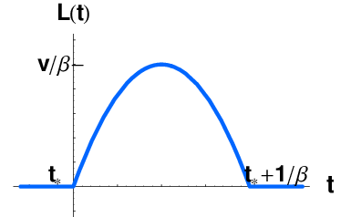
This problem can be fixed by arguing that the pre-factor , instead of being connected to the correlation length as in [6], actually just represents a volume factor connected to the un-collided bubble portion. Therefore, should rather be replaced by , where is a typical shell thickness. In this case the pre-factor becomes . Here is an arbitrary constant which is small in the thin wall approximation, the case considered in simulations. This (somewhat arbitrary) construction leads to
| (37) |
where is given in Eq. (36).
The form of the resulting GW spectrum is shown in Fig. 6.
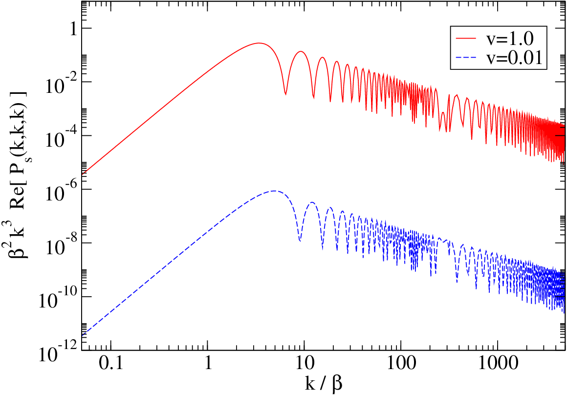
This simple model leads to a velocity independent peak frequency and nicely reproduces the decay for large frequencies in accordance with the results from simulations [5]. In particular, there is no additional suppression at very large frequencies, . The oscillatory behavior should vanish if averaged over several bubbles with slightly different nucleation times and sizes.
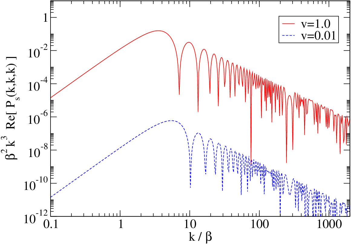
Even though this model reproduces all qualitative features found in the simulations of bubble collisions in the envelope approximation, this analysis should not be understood as a derivation, since some features of the spectrum result from the judicious choice made in Eq. (37), as we have argued above. For example, if we choose to replace in the pre-factor by , which seems more consistent, we obtain a behavior for large since the time-dependence is now , see Fig. 7.
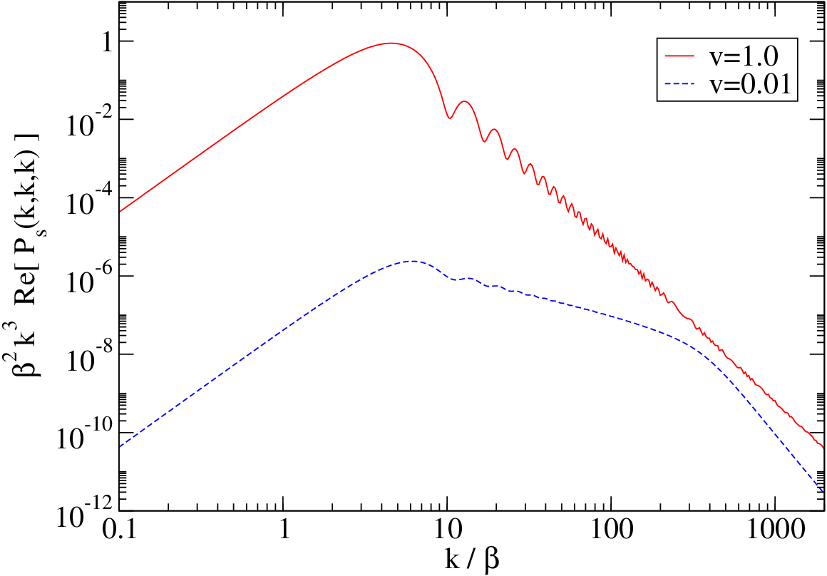
On the other hand, if we argue that the correlation scale should be the size of the largest bubbles as in [6], and we just fix the discontinuity problem by
| (38) |
the spectrum has a peak at , a behavior between and , and an additional kink at beyond which it decays more rapidly, see Fig. 8.
Let us compare these findings with the results of [6]. First, we want to stress that bubble collisions in the approach of Ref. [6] are modeled using Wick’s theorem. The anisotropic stress correlator comes from the product of four velocities,
| (39) | |||||
where and the velocity correlator is non-vanishing only if and are in the same bubble. Thus, the above products are non-zero if and are in the same bubble with center, say for the first factor and with center for the second factor. The probability that is vanishingly small. Hence and belong to two different bubbles which therefore must overlap. In this treatment, the scale associated with is the size of the overlapping region which is of the order of the size of a typical bubble, . The only difference between the approach followed in Ref. [6] and the Ansatz in Eq. (38) is the pre-factor . This pre-factor is nevertheless quite important since it renders the anisotropic stress continuous in time. In Ref. [6] the anisotropic stress is an increasing function up to the end of the phase transition and is then abruptly set to zero. For the coherent case, this modifies the spectrum especially between and , since the high frequency behavior of a discontinuous function goes like . For this reason, in the totally coherent approximation which is relevant here, the gravitational wave power spectrum found in Ref. [6] grows like in the interval and decays only for , leading to a peak at (cf. Fig. 3). This behavior is seen only if the stresses build up dominantly towards the end of the transition, something that is not seen in the simulations. Once this discontinuity is removed by e.g. multiplying with , the treatment proposed in Ref. [6] turns into the spectrum shown in Fig 8, for which the peak is at (cf. also Fig. 3), but which still has a kink at . This kink does not appear in the simulations.
The simulations discussed in [5] show two major differences with respect to the analytic modeling presented in Ref. [6]. First, in the simulations, the anisotropic stress correlator goes to zero at the end of the transition and does not decay abruptly as assumed in the analytical modeling. Furthermore, the typical scale which enters the spectrum is not the size of the bubbles as assumed in the analytical modeling, but it is the size of the not yet collided region of overlapping bubbles. This size starts small, reflecting the initial smallness of the bubbles, and goes to zero towards the end of the transition when most bubbles are nearly fully collided.
In order to account for these differences, and recover the same result for the GW spectrum, we can modify the analytical model in [6] as explained above, leading to Eq. (37). It is important to remark that the most obvious treatment of the volume factor as does not lead to the spectrum obtained in the simulations. To recover the results of the simulations, the shell thickness has to be introduced. This is not surprising, since the simulations are performed in the envelope approximation.
Note also that the behavior found in the simulations is very sensitive to the time differentiability of the spatial Fourier transform of an average collision event, the function . This function has to be in but not in . The derivative has to have a jump (but not a divergence) at either or , and the non-vanishing slope of the right-side derivative at (or left-side at ) may not depend on . This behavior can be modeled with Eq. (37) where it is important not only that goes to zero in a continuous but non differentiable way at both ends of the phase transition, but also that the -dependence of vanishes at these times.
Finally, let us estimate the constant of proportionality between the GW spectrum and the anisotropic stress . The total, dimensionless anisotropic stress density for a typical bubble collision event is of the order
| (40) |
where denotes the fraction of the latent heat that is transformed into kinetic bulk motion of the plasma and finally into anisotropic stress [2]. For infinitely thin bubbles in vacuum, where only the Higgs field plays a role, and . If the phase transition happens in a thermal bath, , where denotes the typical velocity of the thermal bath particles resulting from the interaction with the bubble wall. The volume of a typical bubble is given by
| (41) |
When calculating the space Fourier transform of (40) we obtain a volume factor of the order of the size of the bubble. Furthermore, the time integration gives roughly a factor so that we have
| (42) |
Inserting this in the anisotropic stress power spectrum Eq. (34) yields
| (43) |
For the gravitational wave energy density given in Eq. (10) this yields, together with the typical behavior in the wavenumber obtained from the numerical simulations and from the modeling leading to Fig 6,
For small wall velocities , the wavenumber of the peak is roughly constant , while a slight dependence on the velocity is observed in the simulation result for big velocities.
Note, however, that the velocity relating the characteristic scale and the characteristic time corresponds to the speed of the bubble wall only if the phase transition proceeds through detonations. In this case, is anyway larger than the relativistic speed of sound, . In the deflagration case, on the other hand, the speed of the bubble wall is subsonic, and the bubble is preceded by a shock wave in the symmetric phase (while the broken phase fluid is at rest). It is the collision of these shock waves that eventually leads to the generation of gravitational waves. Therefore, also in the deflagration case, the velocity relating the characteristic length and time scales of the problem is supersonic (since it corresponds to the front of a shock wave) [6]. In summary, values of smaller than the relativistic speed of sound are not realistic, and have been considered here just for illustrative purposes. This means that the difference in the peak position between the analytical and the simulation result, although conceptually relevant, is probably negligible from the point of view of observations. However, it is important to notice that since the simulations are carried out in the envelope approximation, they can only model the detonation case and are valid under the assumption of supersonic velocities of the bubble wall.
V Conclusions
In this paper we have discussed some general considerations which determine the spectrum of gravitational waves from a phase transition, or from some other short-lasting cosmological events which leads to the formation of anisotropic stresses. A first, relatively known result is that the gravitational wave energy spectrum, always grows like on large scale, i.e. scales much larger than all scales in the problem. Furthermore we have seen that, if the unequal time correlator of the anisotropic stress is totally incoherent or coherent only over less than one wavelength, the time structure of the event does not affect the spectral shape, which is then entirely given by the spatial structure of the correlator. This situation changes if the source is close to totally coherent. Then the spectrum changes at the characteristic time scale of the problem to turn from to
- 1.
, if the anisotropic stress correlator is discontinuous (in time) at the beginning (or the end) of the source.
- 2.
, if the anisotropic stress correlator is but the first derivative jumps at the beginning (or the end) of the source.
- 3.
, if the anisotropic stress correlator is but the second derivative jumps at the beginning (or the end) of the source.
These slope changes are realized if the jump height is independent of ; otherwise, the result is more complicated. In case 1, an additional change of slope is needed at the typical spatial scale of the problem, for the total energy density to remain finite. Whether there is an additional change of slope in the other cases depends on the details. If the spatial structure does not have any intrinsic time dependence, i.e. in the separable case (14), this is certainly expected. However if the typical spatial scale of the problem depends on time this may affect the decay for large .
Numerical simulations [5] indicate that for gravitational waves from colliding bubbles the second case above is realized, in such a way that there is no additional change of slope at higher frequencies. This is because the typical spatial scale of the source tends to zero also at the end of the phase transition. This result, which is at odds with the naive expectation that the typical scale would be the bubble size, (which tends to at the end of the transition) is quite important. It implies a mild decay of the gravitational wave signal at high frequency which is most relevant for the detectability of the corresponding gravitational waves, e.g. from the electroweak phase transition (see Ref. [5]).
In the simulations, the typical spatial scale of the problem is connected to the portions of un-collided bubble wall at a given time, and therefore goes to zero both at the beginning (when bubbles have not yet started to collide) and at the end of the phase transition. The statistical average is then performed by averaging the GW emitted by a given realization over several directions. On the other hand, in the analytical approach followed in [6], the characteristic randomness of the problem is assumed from the beginning. Therefore, what matters are correlation lengths, and the most obvious correlation length of the problem is given by the bubble size. This is so in the analytical approach of [6] which models the ‘overlap’ of bubbles, and not directly the ‘collisions’. In contrast, in the simulations, the bubble size does not appear as an important scale of the problem. Therefore, in order to recover the simulation results from the analytical model, one needs to identify the size of portions of un-collided bubble wall as the relevant characteristic scale. Consequently, the ‘volume’ factor coming from the spatial Fourier transform (cf. Eq. (35)) also has to be modified; however, this cannot be done simply by setting it to the un-collided bubble portion size cubed. To recover the simulation spectrum, the portions of uncollided bubble wall must only enter as a surface portion, while the thickness should be taken as an independent constant. This is to be understood in the context of the thin wall approximation used in the simulations. Taking into account a time dependent finite thickness of the shell of stress would tame the kinks in Fig. 5 and also introduce an additional length scale in the GW spectrum. Consequently, using a finite wall thickness in the simulations would most probably lead to a steeper slope in the GW spectrum compared to the result in the thin wall approximation for . Accounting for a finite wall thickness in the analytic approach [6] leads to the same result, but the steeper slope starts at (cf. Eq. 38 and Fig. 8).
It will be important to study the implications of these results for the production of gravitational waves from turbulence and from stochastic magnetic fields. In the first case, the typical spatial scale of the problem most probably does not tend to zero at the end of the turbulent phase, while magnetic fields are likely to be long-lived and therefore have to be treated differently.
Acknowledgment
This work is supported by the Swiss National Science Foundation. TK acknowledges support by the Marie Curie Research & Training Network ”UniverseNet”. CC and GS acknowledge support from the ANR funding DARKPHYS.
References
- [1]
S. Y. Khlebnikov and I. I. Tkachev, Phys. Rev. D 56 (1997) 653
[arXiv:hep-ph/9701423];
R. Easther and E. A. Lim, JCAP 0604 (2006) 010 [arXiv:astro-ph/0601617 ];
R. Easther, J. T. Giblin and E. A. Lim, Phys. Rev. Lett. 99, 221301 (2007) [arXiv:astro-ph/0612294];
Juan Garcia-Bellido, Daniel G. Figueroa, Phys. Rev. Lett. 98, 061302 (2007) [arXiv:astro-ph/0701014];
J. Garcia-Bellido, D. G. Figueroa and A. Sastre, Phys. Rev. D 77, 043517 (2008) [arXiv:0707.0839 ];
Jean Francois Dufaux et al., Phys. Rev. D 76, 123517 (2007) [arXiv:0707.0875]. - [2]
A. Kosowsky, M. S. Turner and R. Watkins, Phys. Rev. D 45, 4514 (1992);
A. Kosowsky and M. S. Turner, Phys. Rev. D 47, 4372 (1993) [arXiv:astro-ph/9211004 ];
M. Kamionkowski, A. Kosowsky and M. S. Turner, Phys. Rev. D 49, 2837 (1994) [arXiv:astro-ph/9310044 ];
A. Kosowsky, A. Mack and T. Kahniashvili, Phys. Rev. D 66, 024030 (2002) [arXiv:astro-ph/0111483 ];
C. Grojean and G. Servant, Phys. Rev. D 75, 043507 (2007) [arXiv:hep-ph/0607107];
C. Caprini and R. Durrer, Phys. Rev. D 74, 063521 (2006) [arXiv:astro-ph/0603476 ];
T. Kahniashvili, A. Kosowsky, G. Gogoberidze and Y. Maravin, Phys. Rev. D 78, 043003 (2008) [arXiv:0806.0293 [astro-ph]]. - [3] A. Kosowsky and M. S. Turner, Phys. Rev. D 47, 4372 (1993) [arXiv:astro-ph/9211004].
- [4] M. Kamionkowski, A. Kosowsky and M. S. Turner, Phys. Rev. D 49, 2837 (1994) [arXiv:astro-ph/9310044 ].
- [5] S. J. Huber and T. Konstandin, JCAP 0809, 022 (2008) [arXiv:0806.1828 [hep-ph]].
- [6] C. Caprini, R. Durrer and G. Servant, Phys. Rev. D 77, 124015 (2008) [arXiv:0711.2593 [astro-ph]].
- [7] C. Caprini and R. Durrer, Phys. Rev. D 74, 063521 (2006) [arXiv:astro-ph/0603476].
- [8] C. Caprini, R. Durrer and R. Sturani, Phys. Rev. D 74, 127501 (2006) [astro-ph/0607651].
- [9] S. Weinberg, “Gravitation and Cosmology,” Wiley, New York (1982).
- [10] R. Durrer and C. Caprini, JCAP 11, 10 (2003).
- [11]
G. Gogoberidze, T. Kahniashvili and A. Kosowsky,
Phys. Rev. D 76, 083002 (2007)
[arXiv:0705.1733 [astro-ph]];
T. Kahniashvili, L. Campanelli, G. Gogoberidze and B. Ratra, Phys. Rev. D 78, 123006 (2008) [arXiv:0809.1899 [astro-ph]].