Equations (8), (9) and (10) are written in the dark matter rest frame. However, a priori, the dark energy sound speed, $c_{s\,de}^{2}=\frac{\delta P_{de}}{\delta\rho_{de}}$, is only well known in the rest frame of dark energy [26]. It can be shown [26] that:

where $\hat{c}_{s\,de}^{2}$ is the propagation speed of pressure fluctuations in the rest frame of dark energy and $c_{a\,de}^{2}=\dot{P}_{de}/\dot{\rho}_{de}$ is the so called “adiabatic sound speed”, which for constant $w$ satisfies $c_{a\,de}^{2}=w$. In the presence of a dark coupling, from Eqs. (4) and (11) it follows that

where we define

where ${\bf d}$ stands for doom: we dub it so as it is precisely this extra factor, proportional to the dark coupling $Q$, which may induce non-adiabatic instabilities in the evolution of dark energy perturbations. Its sign will be determinant, as we are going to show.

Rewriting Eqs. (8), (9) and (10) in terms of $\hat{c}_{s\,de}^{2}$ and ${\bf d}$, we have:

where $\delta[\,{\bf d}\,]$ includes $\delta Q$ and $\delta_{de}$ contributions.

Below, in addition to $w<-1/3$, the speed of sound $\hat{c}_{s\,de}^{2}$ will be assumed positive, with $\hat{c}_{s\,de}^{2}=1$ in numerical computations.

In general, the evolution of the dark energy and the dark matter perturbations are directly coupled. Indeed, it is known that, even in the uncoupled case, once $w\neq-1$ the dark matter and dark energy perturbation evolution depend on each other [27] (see also Sec. 2.3).

When the dark fluid linear perturbation equations are combined into second order differential equations, they take the generic form ⁸⁸ 8 We surrender here to the extend habit of expressing first order temporal differential equations in terms of conformal time, $\dot{\,}=\partial/\partial\tau$, while in second order ones ${}^{\prime}\,=\partial/\partial\,a$ is used.:

where ${}^{\prime}=\,\partial/\partial a$ and the function $\mathcal{F}$ ($\mathcal{G}$) stores the dependence in all variables but $\delta_{dm}$ or $\delta_{dm}^{\prime}$ ($\delta_{de}$ or $\delta_{de}^{\prime}$).

The evolution of a perturbation will depend on the relative weight of the three terms in the corresponding equation and on their signs:

1. 1.

   For positive $A$, the $A$ and $B$ terms taken by themselves would induce a rapid growth of the perturbation, which may be damped or antidamped (reinforced) depending on whether $B$ is negative or positive, respectively ⁹⁹ 9 Obviously, for $|B|>>|A|$ a negative $B$ would prevent the onset of growth for any sign of $A$.. In particular, for $A$ and $B$ both positive, the solution may enter in an exponentially growing, unstable, regime.

2. 2.

   For negative $A$, in contrast, the $A$ and $B$ terms taken alone describe a harmonic oscillator, with oscillations damped (antidamped) if $B$ is negative (positive). In the $A,B<0$ regime, the third term may plays in fact the leading role.

It is worth reviewing the uncoupled scenario in detail before proceeding further: in it, dark matter perturbations behave as in case 9 above (with $A>0$ and $B<0$), while dark energy ones provide an example of behavior as in case 2.

Consider first the growth of dark matter and dark energy density perturbations, in the absence of dark coupling ($Q=0$), at large scales (${\mathcal{H}}/k^{2}\ll 1$) and early times, when $\Omega_{de}\delta_{de}$ can be neglected as $\Omega_{de}\ll\Omega_{i}$ for $i=$ all other species. In this regime,

with the functions $\mathcal{F}$ and $\mathcal{G}$ are given by:

Equation (19) for dark matter density perturbations has $A>0$ and $B<0$: the latter term damps the growth of dark matter perturbations propitiated by the $A$ term, with the overall well known polynomial rising, see Fig. 1 (left panel) .

Equation (20) for dark energy perturbations has instead both $A$ and $B$ coefficients negative, with the first two terms describing then a damped harmonic oscillator and in this case the contribution of radiation, dark matter and matter encoded in $\mathcal{G}$ drives the evolution, see Fig. 1 (right panel). Equations (20) and (22) also illustrate that, for constant $w\neq-1$, dark energy perturbations do develop even in absence of coupling, seeded by the $\mathcal{G}$ term, in contrast to the $w=-1$ (pure vacuum energy) case, in which no perturbation can develop in the dark energy background.

Consider now the opposite case in which the dark-coupling terms dominate over the usual one. For $\hat{c}_{s\,de}^{2}>0$ considered all through, the strong coupling regime can be characterized by

which guarantees that the interaction among the two dark sectors drives the non-adiabatic contribution to the dark energy pressure wave, see Eq. (12), and becomes the leading term in Eq. (15) for $\dot{\delta}_{de}$ and Eq. (16) for $\dot{\theta}_{de}$. At large scales, those equations reduce to:

The complete second order differential equation describing the growth of dark energy perturbations can be found in Appendix A; for values of $w$ near $-1$ and in the strong coupling regime, the $\delta_{de}$ and $\delta_{de}^{\prime}$ contribution to the second order differential equation reads

The sign of the coefficient $B_{e}$ of $\delta_{de}^{\prime}$ in this expression is crucial for the analysis of instabilities, as previously argued, see Eq. (18). Notice that the size and sign of the $B_{e}$ coefficient also determines the growth rate of $\theta_{e}$ in Eq. (25). Assuming $\hat{c}_{sde}^{2}>0$, it reduces to the sign of the doom factor ${\bf d}$ defined in Eq. (13).

Indeed, as previously argued, a positive ${\bf d}$ acts as an antidamping source in the growth Eq. (26). Whenever ${\bf d}>1$, it will trigger an exponential runaway growth of the dark energy perturbations when simultaneously the overall sign of the $A_{e}$ coefficient of $\delta_{de}$, resulting from the last two terms in Eq. (26), is also positive. Large scale instabilities arise then and the universe appears to be nonviable.

The dark matter and dark energy background densities evolve in this model as two fluids, coupled with a strength linearly dependent on the dark energy density present at any given time of the cosmic evolution,

which then correspond to two fluids with effective equations of state given by

Note that for constant $w$, $w_{de}^{eff}$ is also constant while $w_{dm}^{eff}$ is redshift dependent. The solutions to equations (3) and (4) are then:

The dark energy density is thus always positive, all along the cosmic evolution and since its initial moment. To ensure that the same happens with the dark matter density, all values of $w<0$ are acceptable for $\xi<0$, while for positive $\xi$ it is required that $\xi\lower 3.22916pt\hbox{$\sim$}\hbox to0.0pt{\hss\raise 1.1625pt\hbox{$<$}}-w$.

The resulting evolution of the relative energy densities is shown in Fig. 2, where the present matter and dark energy densities have been imposed to be $0.27$ and $0.73$ (a procedure to be repeated all through the paper). We see that negative (positive) couplings lead to more (less) dark matter in the past than in the uncoupled case, as expected. As a consequence, the matter radiation equality happens earlier (later) on. Fig. (2) illustrates as well that positive (negative) values of $Q$ soften (worsen) the coincidence problem, although the difference turns out to be quantitatively minor for the phenomenologically allowed values of $\xi$. It will be shown in Sect. 3.5 that models with $\xi<0$ and $1+w>0$ will give the best agreement with large scale structures observations.

Finally, Eqs. (32) and (34) show that the so-called phantom regime, in which the dark energy density would diverge in the future, can only happen in this model for $1+w^{eff}_{de}<0$, that is, for $w<-1-\xi/3$, instead of $w<-1$ in the uncoupled case.

From the previous analysis one can wonder what would be the dark energy equation of state reconstructed from observational data, if analyzed assuming no coupling. Indeed a dynamical, redshift-dependent, equation of state $\tilde{w}(z)$ (where $z$ denotes redshift), can be mimicked by the combination of constant $w$ plus the dark coupling $\xi$ .

A wealth of data are sensitive to the Hubble parameter $H(z)$ or functions of its integral. When such data are analyzed assuming no dark coupling, the following expression for the Friedmann equation is to be considered ¹⁰¹⁰ 10 We obviate here as well, for the sake of the argument, the contribution to $\Omega^{(0)}_{TOT}$ of any species other than dark matter and dark energy: baryons, neutrinos and curvature.:

where $\Omega^{(0)}_{i}=\rho^{(0)}_{i}/\rho^{(0)}_{c}$, being $\rho^{(0)}_{c}$ the critical energy density today. Relation (35) can be inverted to obtain $\tilde{w}(z)$ as a function of $R_{H}(z)$:

An analogous relation between the redshift dependent equation of state and the luminosity distance and its derivative was also obtained previously [32].

In contrast, in the presence of the dark coupling, from Eqs. (33) and (34) it results for the simple model analyzed in this section

Comparing Eqs. (35) and (37), it follows the relation between the hypothetically reconstructed expression of a dynamical equation of state $\tilde{w}(z)$ and the constant $w,\xi$ parameters of the darkly coupled universe:

an expression which at small redshifts tends to:

while $\tilde{w}(z)\rightarrow 0$ at very large redshifts.

A striking implication of Eq. (38) is that the reconstructed equation of state would show a peculiar divergent behavior for those models in which the denominator vanishes. In fact, for modified gravity models and coupled scalar-tensor models a similar behavior was previously pointed out [33, 34]: their reconstructed $\tilde{w}(z)$ could appear singular at some point in the past and cross the “phantom boundary” $w=-1$.

In the phenomenologically viable model discussed here no such divergent behavior can arise in the $\tilde{w}(z)$ reconstruction, for negative values of the dark coupling $\xi$ for any $w<0$. Whereas, for positive dark coupling values, a “phantom-like” behavior appears, with the divergence occurring at redshift $z\sim{\mathcal{O}}(1-10)$, depending on the specific values of the parameters.

All these different behaviors are illustrated in Fig. 3, for $w=-0.9$ and $\xi=\pm 0.8,\pm 0.2$. The model with $w=-0.9$ and $\xi=0.8$ is not viable, due to negative dark matter energy density, and it is shown only for illustration purposes.

Notice that an apparently diverging behavior of the equation of state could thus be a clean indicator of the sign of a putative dark coupling. Furthermore, the degeneracy between a dynamical equation of state and a constant $w$ plus dark coupling, discussed in this subsection, can be disentangled with other $z-$sensitive data, such as precision BAO or SuperNovae measurements and the growth of perturbations seeding large structure formation, as it will be seen in Sec. 3.5.

The propagation of dark energy pressure waves is driven by Eq. (12) as explained above, with the doom factor Eq. (13) given in this case by:

The evolution of the perturbations, in the synchronous comoving gauge, is described by Eqs. (14), (15) and (16) with, in the present scenario,

The dark matter density perturbation changes in size with respect to the uncoupled case. It is easy to confirm numerically that the major effect of the coupling on the dark matter distribution results from the background, though, for dark coupling values small enough so as to allow viable models. For negative couplings, there is more dark matter in the past. As a consequence, dark matter perturbations cluster more and the density perturbation is larger.

The strong coupling regime is defined by $|{\bf d}|>1$, as explained in Sec. 2.4. In this regime and for large scales, $\mathcal{H}/k\gg 1$, the dark energy perturbations are described by Eqs. (24) and (25), where in this case Eqs. (40), (41) and (42) above apply. It leads, for constant $w\neq-1$, to a $\delta_{de}$ and $\delta_{de}^{\prime}$ contribution to the early time growth at large scales, described by

which shows that the sign of ${\bf d}$ defines the (un)stable regimes ¹¹¹¹ 11 Recall that $\hat{c}_{s\,de}^{2}\geq 0$ is assumed all through.:

1. 1.

   For ${\bf d}<0$, that is, for $\xi<0$ and $1+w>0$ (or $\xi>0$ and $1+w<0$), no instabilities are expected;

2. 2.

   When $\xi$ and $1+w$ have the same sign, instabilities can develop at early times whenever ${\bf d}>1$ .

Sweeping over all possible values of $\xi$ and $w$, we have indeed confirmed numerically these predictions. We summarize our instability criteria for the present model in Tab. 1. An example of the onset of unstable behaviour is shown in Fig. 4, right panel, in which the particular choice of $w$ and $\xi$ makes the model unstable at early times, see Tab. 1. The left panel of Fig. 4 depicts instead the dark energy perturbation, $\delta_{de}$, versus the scale factor $a$ in a model free of instabilities and pathological behaviors in the linear perturbation evolution, notwithstanding the strong coupling regime.

In the next subsection, we will confront in detail the model with data, sweeping over values of the dark coupling strength $\xi<0$, although models with $\xi>0$ are also viable as long as $\xi>-w$, as previously shown.

We explore here the current constraints on the dark energy-dark matter coupling $\xi$, considered constant, allowing for a non zero spatial curvature. The framework used is a cosmological model described by ten free parameters,

where $\omega_{b}=\Omega_{b}h^{2}$ and $\omega_{dm}=\Omega_{dm}h^{2}$ are the physical baryon and dark matter densities respectively, $\theta_{CMB}$¹²¹² 12 The $\theta_{CMB}$ parameter can be replaced by the $H_{0}$ parameter. However, using $\theta_{CMB}$ is better due to its smaller correlation with the remaining parameters. is proportional to the ratio of the sound horizon to the angular diameter distance, $\tau$ is the reionisation optical depth, $\Omega_{k}$ is the spatial curvature, $f_{\nu}=\Omega_{\nu}/\Omega_{dm}$ refers to the neutrino fraction, $n_{s}$ is the scalar spectral index and $A_{s}$ the scalar amplitude. The priors adopted on those parameters are given in Tab. 2.

We use the publicly available package cosmomc [35], modifying it in order to include the coupling among the dark matter and dark energy components, for the model considered in this section.

A conservative compendium of cosmological datasets is considered. First, what we call run 0 includes the WMAP 5-year data [1, 2], a prior on the Hubble parameter of $72\pm 8$ km/s/Mpc from the Hubble key project (HST) [36], the constraints coming from the latest compilation of supernovae [3] and the $H(z)$ data¹³¹³ 13 We thank R. Jiménez and L. Verde for suggesting the $H(z)$ data addition to the analysis. at $0<z<1.8$ from galaxy ages obtained by [37]. We present a second data analysis, that we call run I, in which we add to run 0 the data on the matter power spectrum (large scale structure data or LSS data) from the spectroscopic survey of Luminous Red Galaxies (LRGs) from the Sloan Digital Sky Survey (SDSS) survey [4].

In summary,

• •

  run0=WMAP(5yr)+HST+SN +$H(z)$,

• •

  runI=run0+LSS.

Figure 5 (left panel) illustrates the $1$ and $2\sigma$ marginalized contours in the $\xi$–$\Omega_{dm}h^{2}$ plane. The results from the two runs described above are shown. We restrict ourselves here to negative couplings and $w>-1$, which guarantees that instability problems in the dark energy perturbation equations are avoided for all values of $\xi$. Notice that a huge degeneracy is present, being $\xi$ and $\Omega_{dm}h^{2}$ positively correlated. The shape of the contours can be easily understood. In a universe with a negative dark coupling $\xi$, the matter content in the past is higher than in the standard $\Lambda$CDM scenario due to an extra contribution proportional to the dark energy component, see Eq. (33). Therefore, the amount of intrinsic dark matter needed - that is, not including the contribution of dark energy through the coupling term - should decrease as the dark coupling becomes more and more negative and can be as small as 0.02, as indicated by run 0 results. The addition of LSS data to the analysis reduces considerably the allowed parameter space. This is due to the enormous growth of clustering for values of the coupling $\xi<-0.5$. For this range, the amplitude of the fluctuations increases, reaching values of $\sigma_{8}>2$ and therefore providing a bad fit to LSS data¹⁴¹⁴ 14 The authors of Ref. [2] have reported a best fit value $\sigma_{8}=0.812\pm 0.026$..

The right panel of Fig. 5 shows a positive correlation between the coupling $\xi$ and the spatial curvature $\Omega_{k}$. High precision CMB data indicates that currently the spatial curvature is a subdominant contribution to the energy budget of the universe¹⁵¹⁵ 15 The authors of Ref. [38] have found $\Omega^{(0)}_{k}=-0.002^{+0.041}_{-0.032}$ ($95\%$ CL limits) assuming a dynamical dark energy component., which implies $\Omega_{de}^{(0)}+\Omega_{dm}^{(0)}+\Omega_{b}^{(0)}\simeq 1$. A non zero spatial curvature component implies instead $\Omega_{de}^{(0)}+\Omega_{dm}^{(0)}+\Omega_{b}^{(0)}+\Omega^{(0)}_{k}=1$. A negative coupling $\xi$ will increase the dark matter contribution and therefore a small negative curvature (closed universe) is needed to compensate the effect and describe well CMB data. The degeneracy between $\xi$ and $\Omega_{k}$ gets alleviated if one adds LSS data to the analysis.

Figure 6 (left panel) depicts the constraints on the $\xi$–$w$ plane. We restrict ourselves here to $w>-1$ and $\xi<0$, a parameter region which ensures a negative doom factor, see Eq. (40), and thus spans an instability–free region of scenarios to explore (see Sec. 3.4). Current data is unable to set strong constraints on the equation of state parameter $w$.

The right panel of Fig. 6 shows next the correlation among the fraction of matter energy-density in the form of massive neutrinos $f_{\nu}$ and the dark coupling $\xi$. The relation between the neutrino fraction used here $f_{\nu}$ and the neutrino mass for $N_{\nu}$ degenerate neutrinos reads

Neutrinos can indeed play a relevant role in large scale structure formation and leave key signatures in several cosmological data sets, see Ref. [39] and references therein. More specifically, the amount of primordial relativistic neutrinos changes the epoch of the matter-radiation equality, leaving an imprint on both CMB anisotropies (through the so-called Integrated Sachs-Wolfe effect) and on structure formation, while non-relativistic neutrinos in the recent Universe suppress the growth of matter density fluctuations and galaxy clustering. This can be observed in Fig. 7, where the dotted curve depicts the matter power spectrum for three degenerate massive neutrinos ($N_{\nu}=3$) with $m_{\nu}=0.4$ eV. Notice that the matter power spectrum is reduced with respect to the $m_{\nu}=0$ case, especially after the matter–radiation equality era (imprinted in the power spectrum as a turnover).

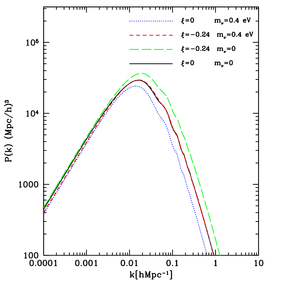There is a strong and very well known degeneracy in the $\sum m_{\nu}-w$ plane, as first noticed in Ref. [40]. Cosmological neutrino mass bounds become weaker if the dark energy equation of state is taken as a free parameter. If $w$ is allowed to vary, $\Omega_{dm}$ can take very high values, as required when $m_{\nu}$ is increased in order to have the same matter power spectrum. More recently, the authors of Ref. [41] have pointed out that a higher neutrino mass is possible if dark matter and dark energy are coupled. Figure 7 shows the matter power spectrum in several scenarios. The long dashed line refers to a universe with three massless neutrinos and a coupling in the dark sector $\xi=-0.24$. Notice that the matter power spectrum is enhanced with respect to the $\xi=0$ scenario, due to the higher matter energy density in models with a non-negligible coupling. However, the power enhancement effect induced by the presence of a coupling can be compensated by adding massive neutrinos in the game. Those neutrinos will reduce the power spectrum, see the short dashed curve in Fig. 7, which is indistinguishable from the matter power spectrum in a $\Lambda$CDM universe. This $m_{\nu}-\xi$ degeneracy is shown in Fig. 6 (right panel): a neutrino mass of $\sum m_{\nu}\sim 1.5$ eV is allowed for couplings $\xi>-0.6$ at the 2$\sigma$ level.

For this scenario, the reconstructed equation of state $\tilde{w}(z)$, if obtained from data mainly sensitive to the fluid background and analyzed assuming no dark coupling, will diverge for positive couplings and redshifts around $z\sim\mathcal{O}(1-10)$. It will show a phantom crossing behavior typical of scalar-tensor dark energy models, see Fig. 9. Indeed using Eq. (36), we get a somewhat more complicated expression than for the $Q\propto\rho_{de}$ scenario:

with $r=\Omega^{(0)}_{de}/\Omega^{(0)}_{dm}$. At small redshifts it reduces to:

while at large redshifts the reconstructed $\tilde{w}(z)$ in Eq. (52) obeys

assuming $|\xi|<1$.

The propagation of dark energy pressure waves is again driven by Eq. (12), with the doom factor Eq. (13) reading now:

This expression should be compared to the analogous one when $Q\propto\rho_{de}$, see Eq.(40): they differ in the $\rho_{dm}/\rho_{de}$ factor in the dark coupling term, which can be large at early times when $\rho_{de}$ may become negligible. At early times, the doom factor will always thus be large even for tiny values of $\xi$, as the ratio $\rho_{dm}/\rho_{de}$ is very large then. This ratio is the major difference between the scenarios with $Q\propto\rho_{dm}$ (or $Q\propto\rho_{dm}+\rho_{de}$ and alike) and those in which $Q\propto\rho_{de}$. As the true expansion factor is ${\bf d}$ instead of $\xi$, this fact also explains why in the present scenario the phenomenological analysis only allows for $\xi$ values much smaller in magnitude than those permitted for $Q\propto\rho_{de}$.

The evolution of the perturbations, in the synchronous comoving gauge, is described in this scenario by Eqs. (14), (15) and (16) with

References

- [1] J. Dunkley et al. Five-Year Wilkinson Microwave Anisotropy Probe (WMAP) Observations: Likelihoods and Parameters from the WMAP data. 2008, 0803.0586.
- [2] E. Komatsu et al. Five-Year Wilkinson Microwave Anisotropy Probe (WMAP) Observations:Cosmological Interpretation. 2008, 0803.0547.
- [3] M. Kowalski et al. Improved Cosmological Constraints from New, Old and Combined Supernova Datasets. 2008, 0804.4142.
- [4] Max Tegmark et al. Cosmological Constraints from the SDSS Luminous Red Galaxies. Phys. Rev., D74:123507, 2006, astro-ph/0608632.
- [5] Will J. Percival et al. The shape of the SDSS DR5 galaxy power spectrum. Astrophys. J., 657:645–663, 2007, astro-ph/0608636.
- [6] R. R. Caldwell, Rahul Dave, and P. J. Steinhardt. Quintessential cosmology: Novel models of cosmological structure formation. Astrophys. Space Sci., 261:303–310, 1998.
- [7] Ivaylo Zlatev, Li-Min Wang, and Paul J. Steinhardt. Quintessence, Cosmic Coincidence, and the Cosmological Constant. Phys. Rev. Lett., 82:896–899, 1999, astro-ph/9807002.
- [8] Li-Min Wang, R. R. Caldwell, J. P. Ostriker, and Paul J. Steinhardt. Cosmic Concordance and Quintessence. Astrophys. J., 530:17–35, 2000, astro-ph/9901388.
- [9] Christof Wetterich. The Cosmon model for an asymptotically vanishing time dependent cosmological ’constant’. Astron. Astrophys., 301:321–328, 1995, hep-th/9408025.
- [10] P. J. E. Peebles and Bharat Ratra. Cosmology with a Time Variable Cosmological Constant. Astrophys. J., 325:L17, 1988.
- [11] Bharat Ratra and P. J. E. Peebles. Cosmological Consequences of a Rolling Homogeneous Scalar Field. Phys. Rev., D37:3406, 1988.
- [12] Sean M. Carroll. Quintessence and the rest of the world. Phys. Rev. Lett., 81:3067–3070, 1998, astro-ph/9806099.
- [13] Luca Amendola. Scaling solutions in general non-minimal coupling theories. Phys. Rev., D60:043501, 1999, astro-ph/9904120.
- [14] Luca Amendola. Perturbations in a coupled scalar field cosmology. Mon. Not. Roy. Astron. Soc., 312:521, 2000, astro-ph/9906073.
- [15] Luca Amendola. Coupled quintessence. Phys. Rev., D62:043511, 2000, astro-ph/9908023.
- [16] D. Comelli, M. Pietroni, and A. Riotto. Dark energy and dark matter. Phys. Lett., B571:115–120, 2003, hep-ph/0302080.
- [17] Subinoy Das, Pier Stefano Corasaniti, and Justin Khoury. Super-acceleration as signature of dark sector interaction. Phys. Rev., D73:083509, 2006, astro-ph/0510628.
- [18] Jussi Valiviita, Elisabetta Majerotto, and Roy Maartens. Instability in interacting dark energy and dark matter fluids. 2008, 0804.0232.
- [19] M. B. Gavela et al. Work in progress.
- [20] Hideo Kodama and Misao Sasaki. Cosmological Perturbation Theory. Prog. Theor. Phys. Suppl., 78:1–166, 1984.
- [21] Rachel Bean, Eanna E. Flanagan, and Mark Trodden. Adiabatic instability in coupled dark energy-dark matter models. 2007, arXiv:0709.1128 [astro-ph].
- [22] E. Lifshitz. On the Gravitational stability of the expanding universe. J. Phys. (USSR), 10:116, 1946.
- [23] E. M. Lifshitz and I. M. Khalatnikov. Investigations in relativistic cosmology. Adv. Phys., 12:185–249, 1963.
- [24] Chung-Pei Ma and Edmund Bertschinger. Cosmological perturbation theory in the synchronous and conformal Newtonian gauges. Astrophys. J., 455:7–25, 1995, astro-ph/9506072.
- [25] Antony Lewis, Anthony Challinor, and Anthony Lasenby. Efficient computation of CMB anisotropies in closed FRW models. Astrophys. J., 538:473–476, 2000, astro-ph/9911177.
- [26] Rachel Bean and Olivier Dore. Probing dark energy perturbations: the dark energy equation of state and speed of sound as measured by WMAP. Phys. Rev., D69:083503, 2004, astro-ph/0307100.
- [27] Jochen Weller and A. M. Lewis. Large Scale Cosmic Microwave Background Anisotropies and Dark Energy. Mon. Not. Roy. Astron. Soc., 346:987–993, 2003, astro-ph/0307104.
- [28] Luca Amendola and Domenico Tocchini-Valentini. Stationary dark energy: the present universe as a global attractor. Phys. Rev., D64:043509, 2001, astro-ph/0011243.
- [29] German Olivares, F. Atrio-Barandela, and D. Pavon. Matter density perturbations in interacting quintessence models. Phys. Rev., D74:043521, 2006, astro-ph/0607604.
- [30] Gabriela Caldera-Cabral, Roy Maartens, and L. Arturo Urena-Lopez. Dynamics of interacting dark energy. 2008, 0812.1827.
- [31] Sergio del Campo, Ramon Herrera, and Diego Pavon. Interacting models may be key to solve the cosmic coincidence problem. 2008, 0812.2210.
- [32] Chris Clarkson, Marina Cortes, and Bruce A. Bassett. Dynamical dark energy or simply cosmic curvature? JCAP, 0708:011, 2007, astro-ph/0702670.
- [33] Luca Amendola and Shinji Tsujikawa. Phantom crossing, equation-of-state singularities, and local gravity constraints in models. Phys. Lett., B660:125–132, 2008, 0705.0396.
- [34] Shinji Tsujikawa, Kotub Uddin, Shuntaro Mizuno, Reza Tavakol, and Jun’ichi Yokoyama. Constraints on scalar-tensor models of dark energy from observational and local gravity tests. Phys. Rev., D77:103009, 2008, 0803.1106.
- [35] Antony Lewis and Sarah Bridle. Cosmological parameters from CMB and other data: a Monte- Carlo approach. Phys. Rev., D66:103511, 2002, astro-ph/0205436.
- [36] W. L. Freedman et al. Final Results from the Hubble Space Telescope Key Project to Measure the Hubble Constant. Astrophys. J., 553:47–72, 2001, astro-ph/0012376.
- [37] Joan Simon, Licia Verde, and Raul Jimenez. Constraints on the redshift dependence of the dark energy potential. Phys. Rev., D71:123001, 2005, astro-ph/0412269.
- [38] Yun Wang and Pia Mukherjee. Observational Constraints on Dark Energy and Cosmic Curvature. Phys. Rev., D76:103533, 2007, astro-ph/0703780.
- [39] Julien Lesgourgues and Sergio Pastor. Massive neutrinos and cosmology. Phys. Rept., 429:307–379, 2006, astro-ph/0603494.
- [40] Steen Hannestad. Neutrino masses and the dark energy equation of state: Relaxing the cosmological neutrino mass bound. Phys. Rev. Lett., 95:221301, 2005, astro-ph/0505551.
- [41] G. La Vacca, S. A. Bonometto, and L. P. L. Colombo. Higher neutrino mass allowed if DM and DE are coupled. 2008, 0810.0127.
- [42] Michel Chevallier and David Polarski. Accelerating universes with scaling dark matter. Int. J. Mod. Phys., D10:213–224, 2001, gr-qc/0009008.
- [43] Eric V. Linder. Exploring the expansion history of the universe. Phys. Rev. Lett., 90:091301, 2003, astro-ph/0208512.
- [44] Work in progress in collaboration with R. Jiménez and L. Verde.