Ambiversion of X(3872)
Ou Zhang,1 C. Meng,1 H. Q. Zheng2
1: Department of Physics, Peking University, Beijing 100871,
China
2: Department of Physics and State Key Laboratory of
Nuclear Physics and Technology, Peking University, Beijing 100871,
China
August 24, 2026
Key words: X(3872); Charmonium; Mesonic molecule
PACS: 13.20.He; 13.25.Gv; 14.40.Lb;
Abstract
An analysis including most recent Belle data on is performed, using coupled channel Flatté formula. A third sheet pole close to but below threshold is found, besides the bound state/virtual state pole discussed in previous literature. The co-existence of two poles near the threshold indicates that the may be of ordinary state origin, distorted by strong coupled channel effects. The latter manifests itself as a molecular bound state (or a virtual state).
1 Introduction
In year 2003 the Belle collaboration found a very narrow ( MeV) resonance structure named X(3872) in the invariant mass spectrum, in the process [1]. The branching ratio is updated to be both by BaBar [2] and by Belle [3]. Moreover, Belle also observed in the decay and found that the rate is comparable with that of the charged channel [3]. Most recently, the CDF Collaboration reported a new measurement on the mass parameter in the channel [4],
| (1) |
Replacing the old CDF measurement by the new one results in a world average of MeV, which is very close to the threshold [5].
The other decay modes of include [6], [7] and [7] with relative rates
| (2) | |||||
| (3) | |||||
| (4) |
The dipion mass spectrum in the mode shows that they come from the resonance [1] and the 3 in the mode come from the resonance [6]. Thus, the rario in (2) indicates that there should be large isospin violation in the decays of .
In year 2006 the Belle collaboration studied the decay process and found the enhancement of the signal just above the threshold [8], the resonance is peaked at
| (5) |
roughly 3.6 MeV higher than the value in (1). The corresponding branching ratio at the peak is [8],
| (6) |
The different peak locations of X(3872) in the () and channels are reconfirmed by latter BaBar experiments [9]. In 2008, a new analysis to the Belle data in the ( and ) channel is given [10], and the new determination of the peak is 2.6MeV lower than the previously reported by Belle [10],
| (7) |
The difference comes from the inclusion of new data (), more sophisticated fit (unbinned fit with mass dependent resolution), and improved Breit–Wigner formula (the Flatté formula). The central value as given by Eq. (7) is, however, still about 1MeV above than the value measured by CDF Collaboration [4]. Meanwhile in Ref. [10] a renewed determination of the following branching ratio is given,
| (8) |
The is naturally interpreted as a molecule of in -wave [11, 12] since its mass is very close to the threshold and the quantum number is favored by the experimental analysis [13]. It also predicted the mode with similar rate as [12]. However, the large production rates of in B-factories and at Tevatron favor a conventional charmonium assignment [14, 15] (say, ) rather than a loosely bound state of . Furthermore, the large decay rate of in (4) also strongly disfavors the molecular assignment since it is very difficult for the transition of a molecular to through the quark annihilation mechanism [12]. The large isospin violation indicated by (2) can also be explained quite well in the charmonium model [16]. Hence it seems that we are facing a dilemma in recognizing .
To further clarify the identity of , one needs to look deeper into the pole structures of the scattering amplitude involving . For a dynamical molecule of , there is only one pole near the threshold, and the requirement of two nearby poles to describe the will generally imply that it is a state near the threshold [17]. The line shapes of in the and modes and the corresponding pole structures have been studied by two groups [18, 19] independently. Both fits give an one-pole structure, although one fit [18] favors a virtual state and the other [19] favors the loosely bound state. Since more data are available after these two fits, it deserves a careful reanalysis to the data of . In this paper we devote to the study of this problem. In Sec. 2, we firstly describe the method we use for the analysis, we also describe how we make the fit from various experimental data. Sec. 3 is for the discussions and conclusions. The final result of this analysis presents a unified picture in understanding the dual faces of : A third sheet pole close to but below threshold is found, besides the bound state/virtual state pole discussed in previous literature. The co-existence of two poles near the threshold indicates that the may be of ordinary state origin, distorted by strong coupled channel effects. The latter manifests itself as a molecular bound state (or a virtual state).
2 Coupled channel description of the X(3872) resonance
Notice that associates with nearby different cuts, hence a coupled channel analysis is needed in order to take care of the complicated singularity structure. This has already been emphasized in Refs. [18, 19, 20, 21]. Hanhart et al. gave a very interesting explanation to the X(3872) peak as a virtual state [18]. Their conclusion relied on of course the experimental data available, and especially on the two peak structure in different channels. The latter plays a crucial role in getting such a conclusion. In the analysis of Hanhart et al., the effect of energy resolution is not considered. Since the two peaks are not too far from each other and the difference between them is comparable in magnitude to the energy resolution parameter, one worries about that the negligence of energy resolution effect may distort their conclusion. For reasons mentioned previously a new analysis on this subject is necessary. We proceed with data prsently available [2, 3, 9, 10] to reanalyze the state, with the energy resolution effect taken into account. On the theory side the method we use is essentially the same as that of Ref. [18].
For describing the chain decays with X(3872) involved as intermediate state, we parameterize the inverse of the propagator of X(3872) as
| (9) |
where ; , and , and are the reduced masses of and , respectively. Isospin symmetry requires . includes channels (through ), (through ) channels. Different from Ref. [18] here we add a constant width to simulate every other channels, including radiative decays and light hadron decays. From Eq. (4) we know that this term is certainly non-negligible as comparing with decay, not to mention the to be observed light hadronic decays.
For simplicity, we describe the and resonances in the final states by their Breit-Wigner distribution functions, then one has
| (10) |
where and are the couplings to and respectively, is the (off-shell) center of mass energy of the X particle and
| (11) |
Let , recalling that , [22] repeatedly using the chain decay formulae leads to,
| (12) |
In the fit to data [9], since all decay modes of are considered there, we drop the factor 0.62 in the first formula of the above equation.
One also has to consider the background contributions. In all the fit to the data, we assume there is no interference between data and background. This is in coincidence with experimental analyses. In channel we assume the background contribution is proportional to , hence
| (13) |
For the final state we assume background contribution is proportional to the phase space of , . In the case, we assume the background is a constant. Herewith we often use overlined branching ratios to represent the signal plus background contributions:
| (14) |
The ratio defined in Eq. (2) has to be put into the fitting program as a constraint. Throughout this paper the ratio is set to 1. The formula used to estimate is the same as that adopted by Hanhart et al. [18], but in here we constrain the value by using the penalty function method, which is simple and effective. That is we effectively add a term to the total : . The factor 10 is an arbitrarily chosen penalty factor which is enough to make the ratio being almost exactly unity. We notice that the ratio measured by experiments contains a large error bar as shown in Eq. (2). We will therefore also pay some attention in the numerical fit to different value of , in next section.
3 The data fitting program and the fit results
3.1 Data samples and the energy resolution parameters
As stated earlier we use 4 sets of data:
- 1:
- 2:
- 3:
Data of from BaBar [2]. We only use the charge mode () data, since the error bar of the neutral mode () data are much larger. There are 11 data points in the fit region GeV and
(16) - 4:
Data of from most recent Belle experiments [3]. We fit the data sample in the energy region from 3.84135GeV to 3.90173GeV, with totally 398 events.
With the unbinned data sets from Belle Collaboration on both from and decay, we make a combined fit of likelihood method and method in the following way:
| (17) |
where ; . The background contributions to the two data samples 2 and 4 are treated similarly as those discussed previously. The PDF used in the likelihood fit is written as,
| (18) |
Because the peaks in different channels are rather close to each other, one needs to take energy resolution effect into account,
| (19) |
In general, the energy resolution parameter is a function of , the original energy of incoming particles. For channel at Belle: For at Belle: [10] We assume that the BaBar detector maintains the same energy resolution parameters.
3.2 Pole locations determined from combined data fit
Experiments indicate to be about a few times . The value of is about in the charmonium model [14], while in the molecular model, it is in general not larger than [19, 23]. Therefore in the following analyses, we often fix at a few times , though it is noticed that the fit program prefers a larger value of with large error bars.
We have stressed in section 2 that we add a constant width term in the Flatté propagator, which corresponds to modes rather than the near threshold ones (). These modes include both the observed ones, such as [7], and the hidden ones. In the charmonium model, the most important hidden decay mode of as is the inclusive light hadronic decay, and the partial width is of MeV [16]. However, for the pure molecule, it is difficult to annihilate the charm quark pair into light hadrons. Therefore, the most important hidden modes of in the molecular model may be the hadronic transitions to , such as and , while the widths of them are expected to be smaller than that of [24]. Thus, the term can provide important information on the .
Poles on different sheets are searched for using results of fit parameters. The naming scheme of Riemann sheets is given in table 1.
| II | III | IV | |
|---|---|---|---|
In table 2 – 5 we list several fit results with different choices of . The error of is given while others are not listed. For comparison we also list the fit results by setting . Notice that in tables 2 – 5 the parameter relates to parameter in Eq. (9) as .
| (GeV) | (MeV) | (MeV) | |||
|---|---|---|---|---|---|
| (MeV) | (MeV) | ||||
|---|---|---|---|---|---|
| (GeV) | (MeV) | (MeV) | |||
|---|---|---|---|---|---|
| (MeV) | (MeV) | ||||
|---|---|---|---|---|---|
By examining the numerical results as given in tables 2–5 we have the following observations:
- 1.
A third sheet pole is always found. When gets large (), the pole locates far away below the threshold. In such a case it is understood that the whole data may well be fitted by a parametrization with a single pole. In this sense, the may be regarded as ‘dynamically generated’. However, for more reasonable choices of (i.e., smaller) , the third sheet pole is rather close to the threshold and is certainly physically relevant.
- 2.
When is small, the fit predicts a value of compatible with the quark model prediction on 2 state light hadronic decay width, i.e., MeV [16].
- 3.
The location of the pole near threshold is not stable in the sense that it may either locate on sheet II or sheet IV. The former corresponds to a molecule, the latter corresponds to a virtual state. The current analysis is not able to make a definite conculsion on the two scenario, though the former is more preferable.
Besides above observations, in the fit when is set to zero, we also confirm the approximate scaling law among different parameters [18]. However, when the constant width is added, the approximate scaling law no longer exists. Because of the approximate scaling law, the authors of Ref. [18] fix one of the parameters (). Their choice is similar to the situation of table 5, corresponding to a large . Hence it explains why in the analysis of Ref. [18] the discussions on the third sheet pole is missed, since the latter is quite distant away from the physical region under concern. However, a choice of seems to be too large to be realistic. A third sheet pole is of typical resonance behavior and can be identified as the missing 2 state. The puzzle remained here is why the third sheet pole locates below the threshold. A pole with such a behavior is sometimes called a “crazy resonance”. [25]
From tables 2–5 we notice that the location of the nearby pole is not very stable numerically, though it seems to prefer to locate on the second sheet (hence a molecule). The second sheet pole may however shift above the threshold, or even switch to sheet IV. Therefore we hesitate to make any definite conclusion on the location of this pole. The only solid statement that can be drawn from above numerical analysis is that the third sheet pole moves towards the threshold and hence becomes non-negligible when parameter is within a few times .


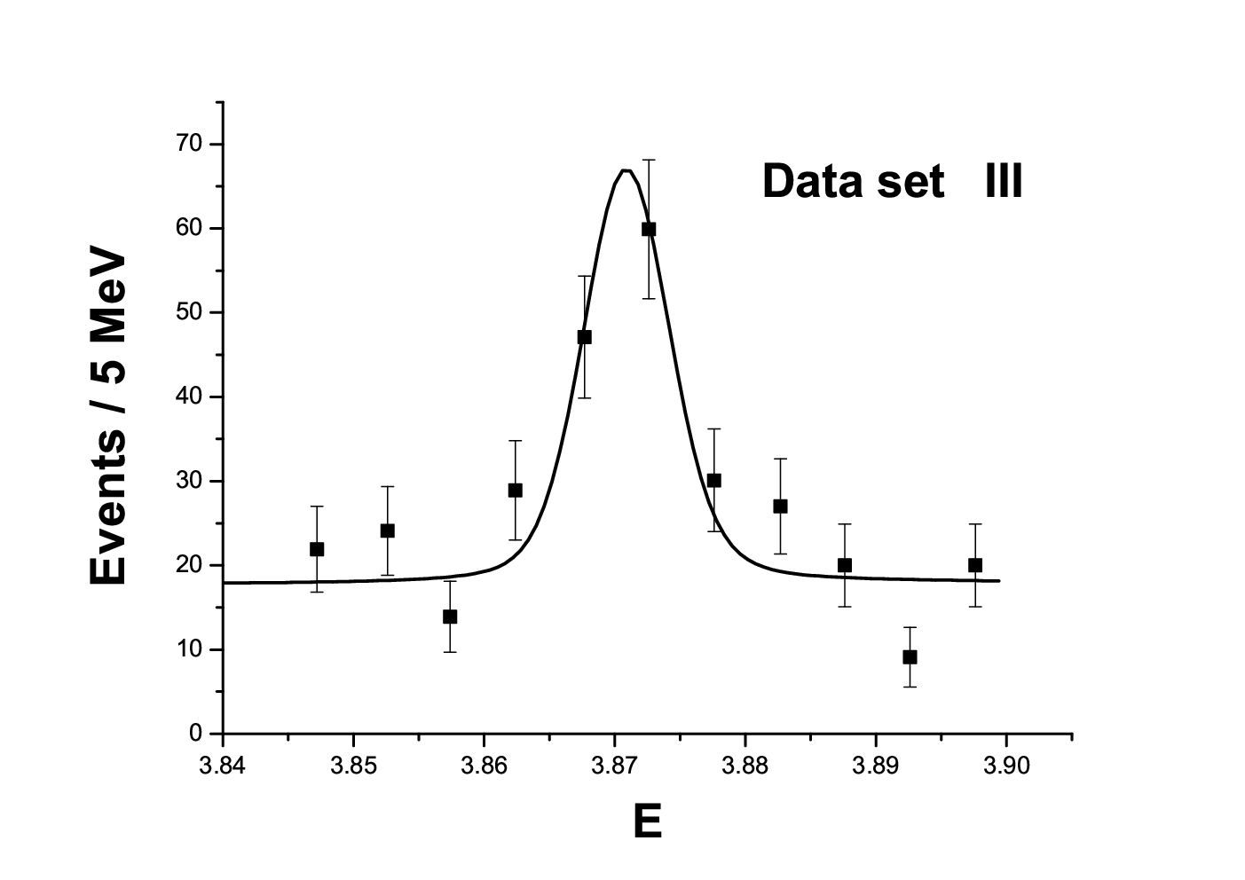

In above an effective minimization procedure with mixed function and likelyhood function is being used. To check weather the qualitative picture revealed depends on the particular choice of Eq. (17) or not, we also tested the binned data fit by taking 1 bin=3.5MeV and fit to the same energy region. It is found that the major conclusion of our qualitative result is unchanged – that a twin–pole structure is needed when is small. Taking for example, the pole locations are found to be: MeV, MeV (with ), to be compared with the results of table 3.
The influence of different choices of the value of defined by Eq. (2) is also tested. Setting and 1.5 for example, it is found that, in all two cases, a third sheet pole a few MeV below threshold is found, except the second sheet pole very close to the threshold. Therefore the variation of ratio does not distort the qualitative picture obtained in our numerical analysis.
4 Discussions and conclusions
It is actually not surprising that our analysis finds two poles – the occurrence of two poles is an intrinsic character of the coupled channel Flatté propagator. The importance of the current analysis is that, as it points out, for reasonably chosen value of , the third sheet pole locates quite close to the threshold and hence be physically relevant, except for the sheet II (or sheet IV) pole emphasized in previous literature. This picture is found to be unaltered when varying the fitting method and the value of . The conclusion certainly depends on the simultaneous fit to experimental data in two channels. The statistics of data set I and II are not as good as the data, hence future improvement on experimental data in and channels would certainly be helpful in clarifying the issue further.
The two pole structure of the state as revealed in this study is important, as we believe, in understanding correctly the nature of the resonance. In this aspect, it can be helpful to learn some lessons from previous studies on the resonance. Generally one pole structure was considered as crucial evidence in supporting the molecule identification of the state in the literature. On the other side, the existence of two poles close to the threshold was often interpreted as an evidence against the molecular state origin of the resonance [17]. Early studies of the tend to identify it as having only one pole near the threshold, and hence a molecular state. [26] It was found later that the scattering data are much better described by allowing two poles near the threshold.[27, 28] In this picture, the third sheet pole may contain a large component, that its position close to the threshold is due to the attractive interaction in the channel. The sheet II pole is mainly of molecule nature. The situation should be rather similar to the case, except that in here the pole locations are distorted more severely by coupled channel effects. What we would like to stress here is that the two pole structure of the state may reveal its dual faces: it is of origin due to the existence of the sheet III pole, but the coupled channel effect also manifests itself by presenting an additional pole, close to the threshold. The latter can also be explained as molecular bound state/virtual state.
It should be stressed that, a pure molecular assignment of encounter a difficulty: the favored value of lead to the width to be roughly of MeV. The pure molecular assignment of , however, would predict a much smaller value of as mentioned earlier. Thus, our analysis supports that is a mixing state of and components [14, 15]. A nearby below threshold is actually reported by quenched lattice QCD calculation. [29] The gap between the mass of in the quark model [30] and the experimental one in Eq. (1) can be reduced when coupled channel effect is taken into account. [31] Here it is worth emphasizing that the shift in the mass of a ‘pure’ is due to the attraction of the threshold, not because of its mixing with other state.
To conclude, the analysis given in this paper suggests the following scenario for : Firstly, there exists a sheet II (or sheet IV) pole very close to the threshold, this confirms previous results in the literature. Secondly, a fit to the data with a reasonable choice of parameter requires the existence of a third sheet pole, but below threshold – this observation is new. With the uncovering of the existence of two poles a clear understanding on the ambiversion of emerges – that it can be identified as a 2 state strongly distorted by coupled channel effects.
5 Acknowledgement
We are grateful to our experimental colleagues, Yuan-Ning Gao and Hai-Bo Li for their kind helps and patient discussions. Especially we are in debt to Steve Olsen, who kindly provides us the original Belle data, for helpful discussions and suggestions. It is also our pleasure to thank Prof. K. T. Chao for helpful discussions. This work is supported in part by National Nature Science Foundation of China under Contract nos. 10575002,10721063, and by China Postdoctoral Science Foundation under contract no. 20080430263.
References
- [1] S. K. Choi et al. (Belle Collaboration), Phys. Rev. Lett. 91(2003) 262001.
- [2] B. Aubert et al. [BaBar Collaboration], Phys. Rev. D 77, 111101 (2008).
- [3] I. Adachi et al. [Belle Collaboration], arXiv: 0809.1224 [hep-ex].
- [4] T. Kuhr, talk given at QWG2008, Nara, Japan, see also the website: http://www-cdf.fnal.gov/physics/new/bottom/080724.blessed-X-Mass.
- [5] C. Cawlfield et al. [CLEO Collaboration], Phys. Rev. Lett. 98(2007) 092002.
- [6] K. Abe et al. (Belle Collaboration), hep-ex/0505037.
- [7] B. Aubert et al. [BaBar Collaboration], arXiv: 0809.0042 [hep-ex].
- [8] G. Gokhroo et al. (Belle Collaboration), Phys. Rev. Lett. 97(2006)162002.
- [9] B. Aubert et al. (BaBar Collaboration), Phys. Rev. D77: 011102(2008).
- [10] I. Adachi et al. [Belle Collaboration], arXiv:0810.0358 [hep-ex]. We thank the Belle group for providing us with the data points used in our fits.
- [11] N.A. Tornqvist, Phys. Lett. B 590, 209 (2004); F. Close and P. Page, Phys. Lett. B 578, 119 (2004); C.Y. Wong, Phys. Rev. C 69, 055202 (2004);E. Braaten and M. Kusunoki Phys. Rev. D 69, 074005 (2004); M.B. Voloshin, Phys. Lett. B 579, 316 (2004).
- [12] E.S. Swanson, Phys. Lett. B 588, 189 (2004); 598, 197 ( 2004).
- [13] K. Abe et al. [Belle Collaboration], arXiv: hep-ex/0505038; A. Aulencia et al. [CDF Collaboration], Phy. Rev. Lett. 96, 102002 (2006); 98, 132002 (2007).
- [14] C. Meng, Y.J. Gao and K.T. Chao, arXiv: hep-ph/0506222.
- [15] M. Suzuki, Phys. Rev. D 72, 114013 (2005).
- [16] C. Meng and K.T. Chao, Phys. Rev. D 75, 114002 (2007).
- [17] D. Morgan, Nucl. Phys. A543, 632 (1992).
- [18] C. Hanhart, Yu. S. Kalashnikova, A. E. Kudryavtsev and A. V. Nefediev, Phys. Rev. D76, 034007 (2007).
- [19] E. Braaten, M. Lu, Phys. Rev. D77, 014029 (2008); Phys. Rev. D76, 094028 (2007).
- [20] D. Bugg, J. Phys. G35, 075005 (2008).
- [21] D. Gammermann, E. Oset, Eur. Phys. J. A36(2008)189; D. Gamermann E. Oset, Eur. Phys. J. A33(2007)119.
- [22] C. Amsler et al. [Particle Data Group Collaboration], Phys. Lett. B 667, 1 (2008).
- [23] E. Braaten, M. Kusunoki and S. Nussinov , Phys. Rev. Lett. 93, 162001 (2004); E. Braaten and M. Kusunoki Phys. Rev. D 71, 074005 (2005).
- [24] M.B. Voloshin, Phys. Lett. B 604, 69 (2004); S. Dubynski and M.B. Voloshin, Phys. Rev. D 77, 014013 (2008); S. Fleming and T. Mehen, Phys. Rev. D 78, 094019 (2008).
- [25] J. Taylor, Scattering Theory, John Wiley & Sons, Inc., New York, 1972.
- [26] J. Weinstein and N. Isgur, Phys. Rev. Lett. 48(1982)659; Phys. Rev. D27(1983)588.
- [27] K. L. Au, D. Morgan and M. R. Pennington, Phys. Rev. D35(1987)1633; D. Morgan and M. R. Pennington, Phys. Rev. D48(1993)1185.
- [28] M. P. Locher, V. E. Markushin, H. Q. Zheng, Euro. Phys. J. C4(1998)317.
- [29] Y. Chen et al. (CLQCD Collaboration), arXive: hep-lat/0701021.
- [30] T. Barnes, S. Godfrey and E.S. Swanson, Phys. Rev. D 72, 054026 (2005).
- [31] B.Q. Li, C. Meng and K.T. Chao, in preparation.