Braid presentation of spatial graphs
Abstract.
We define braid presentation of edge-oriented spatial graphs as a natural generalization of braid presentation of oriented links. We show that every spatial graph has a braid presentation. For an oriented link it is known that the braid index is equal to the minimal number of Seifert circles. We show that an analogy does not hold for spatial graphs.
Key words and phrases:
spatial graph, braid presentation2000 Mathematics Subject Classification
Primary 57M25; Secondary 57M151. Introduction
Throughout this paper we work in the piecewise linear category. Let be a finite edge-oriented graph. Namely consists of finite vertices and finite edges, and each edge has a fixed orientation. Edge-oriented graph is called digraph in graph theory. We consider a graph as a topological space in a usual way. Let be the unit 3-sphere in the -space centered at the origin of . An embedding of into is called a spatial embedding of . Then the image is also called a spatial embedding or a spatial graph. Let (resp. ) be the intersection of and the -plane (resp. -plane). Then the union is a Hopf link in . We call the axis and the core. Let be a natural projection defined by . We give a counter-clockwise orientation to on -plane and fix it. We say that a continuous map is locally orientation preserving if for any edge of and any point on there is a neighbourhood of in such that the restriction map of to is an orientation preserving embedding. Let be a spatial embedding. We say that or its image is a braid presentation if is disjoint from and the composition map is locally orientation preserving where is the map defined by for any in . Note that this generalizes the braid presentation defined for -curve in [5]. The following theorem shows that every edge-oriented spatial graph has a braid presentation up to ambient isotopy of . This generalizes Alexander’s theorem that every oriented link can be expressed by a closed braid [1] and that proved for -curve in [5].
Theorem 1-1.
Let be a finite edge-oriented graph and a spatial embedding. Then there is a braid presentation that is ambient isotopic to in .
In [6] it is shown that the minimal number of Seifert circles of an oriented link is equal to the braid index of the link. We consider an analogy to spatial graphs. Let be a braid presentation. Let for . Let be the maximum of where denotes the cardinality of the set and varies over all points in . Let a spatial embedding. Let be the minimum of where varies over all braid presentation that is ambient isotopic to . We call the braid index of or .
Let be the intersection of and the -space. Then any spatial embedding has a diagram on up to ambient isotopy of . Let be a diagram of on . Let be a plane graph in obtained from by smoothing every crossing of . Here smoothing respect the orientations of the edges. See Figure 1.1.

Let be the number of connected components of a space . Let be the minimum of where varies over all diagrams of up to ambient isotopy of . We call the smoothing index of or . Note that our is different from defined for -curve in [5]. We will show in Proposition 3-1 that for any natural number there is a spatial embedding of with unless contains no cycles as an unoriented graph. In contrast we will show in the next theorem that for any two spatial embeddings and of unless satisfies certain conditions. By (resp. ) we denote the number of the edges whose head (resp. tail) is the vertex of . Then is called the degree of in . We say that an edge-oriented graph is circulating if for any vertex of . Namely each component of a circulating graph is Eulerian. Let be the Euler characteristic of a space . Then we have the following theorem.
Theorem 1-2.
Let be a finite edge-oriented graph without isolated vertices.
(1) Suppose that is not circulating. Then for any spatial embedding , .
(2) Suppose that is circulating. Then for any natural number there is a spatial embedding such that .
Remark 1-3.
Another choice for the smoothing index as a generalization of the number of Seifert circles of an oriented link is the use of the first Betti number instead of the number of connected components. Let be the minimum of among all diagrams of . By the Euler-Poincaré formula we have . Since smoothing does not change the Euler characteristic we have . Then we have . Thus we have that is determined by after all.
2. Proof of Theorem 1-1
The following proof is a natural extension of a proof of Alexander’s theorem by Cromwell [3] using rectangular diagram of oriented links that appears in [2] [3] [4] etc. In this section we regard as a one-point compactification of the -plane. Thus we may suppose that all diagrams are on the -plane. In the following we sometimes do not distinguish an abstract vertex or edge from its image in or on .
Proof of Theorem 1-1. Let be a diagram of the spatial embedding . We will deform step by step so that it is still a diagram of up to ambient isotopy in as follows. First we move if necessary so that is left to the -axis. Namely is contained in the region of the -plane defined by . By a local deformation near each vertex we may suppose that all edges go down with respect to the -coordinate in each small neighbourhood of a vertex of . Then we further deform so that it satisfies the following conditions.
(1) is a union of finitely many line segments.
(2) Each vertex has a small disk neighbourhood such that the diagram on is a union of line segments each of which has as one of its end points, and each of which goes down with respect to the -coordinate.
(3) A line segment that is not contained in any is parallel to -axis or -axis. Then we have that each crossing of is a crossing between a horizontal line segment (parallel to -axis) and a vertical line segment (parallel to -axis). Then by a local deformation as illustrated in Figure 2.1 we may further assume that a horizontal line segment is over a vertical line segment at each crossing. Note that the disk neighbourhood can be taken to be arbitrarily small. Then by a slight deformation we have that a straight line that contains a vertical line segment going up with respect to the -coordinate contains no other vertical line segments and is disjoint from any . Let be the vertical line segments that go up with respect to the -coordinate. We may suppose without loss of generality that the -coordinate of is less than that of if . Let be sufficiently large upright rectangles with and for each . We replace each by that crosses under the horizontal line segments at every crossings. Finally we tilt the horizontal line segments other than slightly so that they go down with respect to the -coordinate. Then we finally have a diagram of that totally turns around the origin of the -plane. Then represents a braid presentation. See for example Figure 2.2. This completes the proof.


3. Proof of Theorem 1-2
A vertex of an edge-oriented graph is called a source (resp. sink) of if (resp. ).
Proposition 3-1.
Let be a finite edge-oriented graph. Suppose that contains a cycle as an unoriented graph. Then for any natural number there is a spatial embedding such that .
Proof. Let be a cycle of . Note that may not be an oriented cycle as an edge-oriented subgraph of . Let be the number of the sources of . Let be a spatial embedding of such that the bridge index of the knot is greater than or equal to . By the definition we have . We may suppose that is a braid presentation with . Then has at most critical points with respect to the -coordinate. Therefore we have . Therefore we have . Thus we have as desired.
Proposition 3-2.
Let be a finite edge-oriented graph and a spatial embedding.Then .
Proof. Let be a diagram of . It is sufficient to show that . Since smoothing does not change the Euler characteristic we have that . Let be the first Betti number of a space . By the Euler-Poincaré formula we have . Therefore we have . Thus we have .
Proof of Theorem 1-2 (1). First we show that . Let be a diagram of . By the definition we have . By Proposition 3-2 we have . Thus we have holds for any diagram of . This implies .
Next we show that has a diagram with . Let be the maximal subgraph of that has no vertices of degree less than 2. If is not an empty graph and is not circulating then we set . Suppose that is an empty graph or a circulating graph. Suppose that there is a component of that is not a component of . Let be the component of containing . Let be an edge of that is not an edge of but incident to a vertex of . Let be the minimal subgraph of that contains and . Suppose that every component of is also a component of . Let be an edge of that is not an edge of . Let be the minimal subgraph of that contains and . Note that in any case we have . Let be the restriction map of the spatial embedding to . We will construct a diagram of with . Namely we will construct such that is connected. We start from a diagram of and deform it step by step and finally have with connected. By Theorem 1-1 we may suppose that is a braid presentation. By deforming the braid presentation if necessary we have that has a diagram on the -plane with the following properties.
(1) There exists a rectangle in the -plane such that at every point on in the edge-orientation goes down with respect to the -coordinate.
(2) Outside of the diagram consists of some parallel arcs turning around the origin of the -plane.
See for example Figure 3.1 (a). In the following deformations we always keep the condition that everything goes down with respect to the -coordinate inside .
Suppose that has some sources and/or sinks. Then by pulling up the sources and moving them to the right as illustrated in Figure 3.2 and pulling down the sinks and moving them to the left we have that all sources are in and all sinks are in and all parallel arcs go left to the sources and go right to the sinks outside of . See for example Figure 3.1 (b).


Then we deform the diagram in such that the following conditions hold.
(1) If a vertex of satisfies then it is rightmost in .
(2) If a vertex of satisfies then it is leftmost in .
See for example Figure 3.3 (a). Now we perform smoothing for the crossings in and obtain on . See for example Figure 3.3 (b) and (c). We do not deform inside any more. We will deform only outside of . However to make the situation simple we further perform the following replacement of on . For each vertex with we replace a neighbourhood of it on by parallel arcs and a vertex with and . Similarly for each vertex with we replace a neighbourhood of it on by parallel arcs and a vertex with and . See Figure 3.4 and Figure 3.3 (d). Then we perform edge contractions if necessary so that there exist at most one vertex, say with and at most one vertex, say with . See for example Figure 3.3 (e). Note that these replacements never decrease the number of connected components. Therefore it is sufficient to show that is connected after these replacements.


Now suppose that there is just one sink of . Let be any point of . We start from along the flow of edge orientations of . If we come across the vertex then we choose the leftmost way. Namely we turn to the right at . Then we see that as we turn around the origin of we move to left and we finally reach to the sink. Thus we have that is arcwise connected. Similarly if there are no sinks of then starting from any point of we finally reach to the outermost circle turning around the origin. Thus is arcwise connected. Suppose that there are at most one source of . Then we see by going against the flow that is arcwise connected. Therefore it is sufficient to consider the case that there are at least two sinks and two sources of . Then by the definition of we have that has no vertices of degree one.
Let be a disk in containing all sinks in its interior. Let be the sinks and , , , ,, , the points of intersection of and such that they appear in this order on , is adjacent to and is adjacent to for each and . See for example Figure 3.1 and Figure 3.5.

We will deform only on . We divide the points , , , ,, , into some sets of points such that for each the points in are consecutive on and any two points in can be connected by an arc in outside . We may suppose without loss of generality that and for each there is a pair of consecutive points on such that one is contained in and the other is contained in where we consider . We will show that contains two or more points possibly except . To see this we start from and trace against the flow. Then we reach to or a source. Then we choose an edge that is next to the edge where we come and along the flow we trace . If we come across then we choose the leftmost way. Then we must reach to or where we consider , and .
Let be a sequence of disks such that their boundaries forms concentric circles in . Let be the annulus.
Suppose that the set is contained in but not contained in . First suppose that the set is a proper subset of . Then we leave in and rename the sinks and the points of intersection of and as illustrated in Figure 3.6. Then we redivide the points , , , ,, , into some sets of points, still denoted by , such that for each the points in are consecutive on and any two points in can be connected by an arc in outside . We may suppose without loss of generality that and for each there is a pair of consecutive points on such that one is contained in and the other is contained in where we consider . Then by the construction we have that contains two or more points possibly except , or except . If contains just one point then we reverse the cyclic order for the next step. Namely we rename again and rename , and rename the points along the new cyclic order on .
Next suppose that the set is equal to the set . Then we deform as illustrated in Figure 3.7 and consider . Note that new and new can be connected by an arc in outside . Therefore we have that each new contains at least two points. Next we deform inside and leave new in in a similar way. We continue this deformation and finally have the desired .
Now we return to the whole graph . Let be the maximal subgraph of that contains and . Let be the tree components of that are disjoint from . Then . Let be the restriction of the spatial embedding to . Let be a diagram of whose subdiagram for is and has no more crossings than . Then we have that and have the same homotopy type. In particular is connected. Let . Let be points on other than the vertices such that is still connected. We may suppose that these points are away from the neighbourhoods of the crossings of where the smoothings are performed. Let be a diagram of whose subdiagram for is such that the crossings of other than that of are exactly the points where the crossing is between an edge of and an edge of . Then we see that . See for example Figure 3.8. Note that we have the following equality.
Therefore if then we have and as desired. If then we have and as desired. This completes the proof.


Proof of Theorem 1-2 (2). Let be an oriented cycle of . Let be a spatial embedding of such that the braid index of the knot is greater than or equal to . Let be any diagram of . It is sufficient to show that . We replace each neighbourhood of a vertex of to oriented arcs as follows. For a vertex that is not on we replace it to mutually disjoint oriented arcs. See for example Figure 3.9. Let be a vertex of that is on . Let be a small neighbourhood of on . Suppose that there is a pair of edges not contained in , say and , such that the head of is , the tail of is and they are next to each other in . Then we take them away from and connect them. We do this for all such pairs. Then we have the situation that all edges in not on go from the right of to the left of or from the left of to the right of . Then we split off them and let goes over them. Let be the result of these replacements. See for example Figure 3.10. Then we have that is a diagram of some oriented link, say . Since contains a knot we have that the braid index of is greater than or equal to . By the result in [6] we have that . Therefore we have . Note that the homotopy type of is obtained from by adding edges where the summation is taken over all vertices of . Therefore we have that . By the handshaking lemma and by the assumption that is circulating we have that . Thus we have as desired.


The following example shows that even for the circulating graphs the difference depends on the spatial embedding .
Example 3-3.
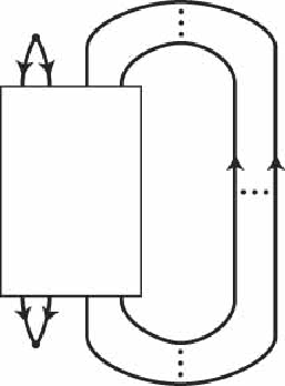
Let be a circulating graph on two vertices and eight edges joining them. Let be a trivial embedding of . Then we have that and . Let be a spatial embedding of illustrated in Figure 3.11. Note that contains a knot that is a connected sum of three figure eight knots. Then we have . Suppose that is a braid presentation as its edge orientations. Then we may suppose that is as illustrated in Figure 3.12 where the box represents some braid. Then we have that . Therefore we have that . Since has two more oriented cycles other than we have that . Since is a braid presentation with we have . However we have that as illustrated in Figure 3.11.

Acknowledgments
The authors are grateful to Professor Shin’ichi Suzuki for his constant guidance and encouragement. The authors are also grateful to Dr. Ryuzo Torii for his helpful comments.
References
- [1] J. Alexander, A lemma on systems of knotted curves, Proc. Natl. Acad. Sci. USA, 9 (1923), 93-95.
- [2] H. Brunn, Uber verknotete Kurven, Verhandlungen des Internationalen Math. Kongresses (Zurich 1897), Leipzig, (1898), 256-259.
- [3] P. Cromwell, Embedding knots and links in an open book I: Basic properties, Topology Appl., 64 (1995), 37-58.
- [4] H. Matsuda and W. Menasco, On rectangular diagrams, Legendrian knots and transverse knots, arXiv:math.GT/0708.2406, 2007.
- [5] T. Shinnoki and T. Takamuki, On the braid index of -curve in 3-space, Math. Nachr., 260 (2003), 84-92.
- [6] S. Yamada, The minimal number of Seifert circles equals the braid index of a link, Invent. Math., 89 (1987), 347-356.