A systematic fitting scheme for caustic-crossing microlensing events
Abstract
We outline a method for fitting binary-lens caustic-crossing microlensing events based on the alternative model parameterisation proposed and detailed in Cassan (2008). As an illustration of our methodology, we present an analysis of OGLE-2007-BLG-472, a double-peaked Galactic microlensing event with a source crossing the whole caustic structure in less than three days. In order to identify all possible models we conduct an extensive search of the parameter space, followed by a refinement of the parameters with a Markov Chain-Monte Carlo algorithm. We find a number of low- regions in the parameter space, which lead to several distinct competitive best models. We examine the parameters for each of them, and estimate their physical properties. We find that our fitting strategy locates several minima that are difficult to find with other modelling strategies and is therefore a more appropriate method to fit this type of events.
Keywords:
gravitational microlensing - data modelling - extrasolar planets - binary stars - robotic telescopes1 Introduction
Gravitational microlensing (Paczyński, 1986) occurs when the light from a source star is deflected by a massive compact object between the source and the observer, leading to an apparent brightening of the source, typically lasting a few days to a few weeks. When the deflecting body has multiple components, such as a planet orbiting its host star, there can be perturbations to the brightening pattern of observed sources. These perturbations can be large even when caused by low-mass objects, making them detectable using small ground-based telescopes. Modelling these lightcurve anomalies can lead to the detection of subtle effects, allowing for measurements of properties such as the source star limb-darkening coefficients (e.g. Cassan et al. 2004), the mass of stars with no visible companions (e.g. Ghosh et al. 2004), and the detection of extrasolar planets, as suggested by Mao & Paczyński (1991) and first achieved in 2003 (Bond et al., 2004).
Nevertheless, anomalous microlensing events usually require very detailed analysis for a full characterisation of their nature to be possible, making them challenging. This applies in particular to a class of microlensing events which display caustic crossing features in their lightcurves. These events are of primary interest, because they account for around ten percent of the overall number of detected microlenses, and they represent an important source of information on physical properties of binary stars (Jaroszynski et al., 2006). However there exist several degeneracies that affect the modelling of this type of events: without a robust modelling scheme and a full exploration of the parameter space, it is impossible to pin down the true nature of a given event. In addition to this, calculations of anomalous microlensing models for extended sources are very demanding computationally.
Given these issues, brute force is not an option when modelling caustic-crossing events, and one has to devise ways of speeding up calculations, for example by excluding regions of parameter space which cannot reproduce features that appear in data sets. A way to achieve this is to use a non-standard parameterisation of the binary-lens models that ties them directly to data features, as proposed by Cassan (2008), which we recall below.
In this paper, we present our method for exploring the parameter space, and describe our approach to find all possible models for a given event (Sec. 2). We then use OGLE-2007-BLG-472, a microlensing event observed in 2007 by the OGLE and PLANET collaborations, as an illustration of our methodology applied on a binary lens event which intrinsically harbors many ambiguities (Sec. 3). We finally discuss the implications of the individual competitive models that we find in order to discriminate between realistic microlensing scenarii.
2 Binary-lens events fitting scheme
2.1 Parameterisation of binary lens lightcurves
A static binary lens is usually described by the mass ratio of the two lens components and by their separation , expressed in units of the angular Einstein radius (Einstein, 1936),
| (1) |
where is the mass of the lens, and and are the distances to the lens and the source respectively. Such a lens produces caustics where the magnification of the source diverges to infinity for a perfect point source. The positions, sizes and shapes of the caustics depend on and . For the binary lens case, caustics can exist in three different topologies, usually referred as close, intermediate and wide; bifurcation values between these topologies are analytical expressions relating with (Erdl & Schneider, 1993). In the close regime, there are three caustics: a central caustic near the primary lens component, and two secondary caustics which lie off the axis passing through both lens components. In the intermediate case, there is only one large caustic on the axis. In the wide case, there is a central as well as a secondary caustic, both on the axis. The limits between these configurations are indicated as the dashed lines in e.g Fig. 2 (see also Fig. 1 of Cassan (2008)).
The description of the lightcurve itself requires four more geometrical parameters in addition to and . In the current standard parameterisation of binary lens lightcurves, these are the source trajectory’s angle with the axis of symmetry of the lens, the time of closest source-lens approach to the binary lens centre-of-mass , the Einstein radius crossing time and the source-lens separation at closest approach (in units of ). Finally for a uniformly bright finite size source star, we add a further parameter, the source size in units of . However, and as discussed in Cassan (2008), this parameterisation is not well adapted to conducting a full search of the parameter space, because the value of the parameters cannot be directly related to features present in the lightcurve, namely caustic crossings for the type of events we are discussing in this paper. Consequently, most of the probed models in a given fitting process do not exhibit the most obvious features in the lightcurve, leading to very inefficient modelling.
To avoid this drawback, Cassan (2008) introduced a new parameterisation in place of and which is closely related to the appearance of caustic crossing features in the lightcurve. The caustic entry is then defined by a date when the source center crosses the caustic11 1 Alternatively, any other point at a fixed position from the source center can be defined as a reference. and its corresponding (two-dimensional) coordinate on the source plane. However, since by definition this point is located on a caustic line, Cassan (2008) introduced a (one-dimensional) curvilinear abscissa which locates the crossing point directly on the caustic, so that . A given caustic structure is fully parameterised by . The caustic entry is then characterised by a pair of parameters , and in the same way the caustic exit by . These four parameters (in addition to and ) which describe the caustic crossings therefore also define an alternative parameterisation of the binary lens, far better fitted to describing the problem at hand.
2.2 Exploration of the parameter space
We start by exploring a wide region of the parameter space with a grid regularly sampled in logarithmic scale. This choice comes from the fact that the size of the caustic structures behave like power-laws of the lens separation and mass ratio, and so do the corresponding lightcurve anomalies. We fit for the remaining model parameters , , , and , being held fixed. From this, we then build a map that we use to locate the best-fit -regions. As mentioned previously, there exist binary lens configurations which involve central and secondary caustics. In these cases (i.e. in the wide and close binary cases) and following Cassan (2008), we study separately models where the source crosses the central or the secondary caustic by building two maps, corresponding to each configuration.
In order to sample efficiently and extensively and (which determine the source trajectory), we use a genetic algorithm (Charbonneau, 1995, e.g.) that always keeps the best model from one generation to the next one (elitism). In fact, since we consider only models displaying caustics at the right positions, there are a couple of local minima associated with different pairs which would usually be missed by other minimisation methods, while a genetic algorithm naturally solves this problem in an efficient way. However, since such an algorithm never converges exactly to the best model, we finally refine the model by performing a Markov-Chain Monte-Carlo (hereafter MCMC) fit: we start several chains and use the criterion by Geweke (1992) to assess convergence to a stationary posterior distribution of the parameter probability densities.
From the obtained maps, we then identify all the local minima regions and use the corresponding best models found on the grid as starting points to refine the parameters, including that we now allow to vary. Since the fit is performed within a minimum region, the fitting process is very stable and fast.
3 Application to OGLE-2007-BLG-472
3.1 Alert and photometric follow-up
On 19 August 2007, the OGLE Early Warning System (Udalski, 2003) flagged microlensing candidate event OGLE-2007-BLG-472 at right ascension 17:57:04.34, and declination -28:22:02.1 or , .

The OGLE lightcurve has an instrumental baseline magnitude I=16.00, which may differ from the calibrated magnitude by as much as 0.5 magnitudes. Lensing by the star in the point source-point lens (hereafter PSPL) approximation accounts for a broad rise and fall in the lightcurve, peaking around MHJD22 2 MHJD=HJD-2450000=4334.0 with an apparent half-width at half-peak of about 10 days (Fig. 1). Although the observed OGLE flux rises only by 0.06 mag in the non-anomalous part of the lightcurve, the shape of the curve hints that blending is important for this target, with only 12% of the baseline flux due to the un-magnified source.
On 19 August (MHJD=4331.5) an OGLE data point showed sudden brightening of the source, with subsequent PLANET (UTas Mt. Canopus 1.0m telescope in Tasmania and Danish 1.54m telescope at La Silla, Chile) and OGLE data indicating what appears to be a fold caustic crossing by the source, ending with a PLANET UTas data point on August 21 (MHJD=4334.1). The caustic entry is observed by a single OGLE point, while the caustic exit is well covered by our UTas data set (Fig. 1). Treating the lightcurve as the addition of an anomaly to a PSPL lightcurve, the underlying PSPL curve then apparently reaches peak magnification on August 22 (MHJD=4335.45). Particularly crucial in our data set is the UTas observation taken within a few hours of the caustic exit, which puts constraints on the position of the caustic exit on the lightcurve, and on the size of the source. Although some V-band observations were taken, the V lightcurve of this event is flat and does not allow us to place constraints on the V flux parameters.
| Telescope | Data | Error bar rescaling factor |
|---|---|---|
| UTas 1.0m | 34 | 1.79 |
| Danish 1.54m | 84 | 1.55 |
| OGLE | 857 | 1.21 |
3.2 Data reduction
We reduced the PLANET data for this event using the data reduction pipeline pysis3.0 (Albrow 2008). This pipeline uses a kernel as a discrete pixel array, as proposed by Bramich (2008), rather than a linear combination of basis functions.This has the advantage that it removes the need for the user to select basis functions manually, which can lead to problems if inappropriate functions are chosen. In addition to this, the pixel array kernel copes better with images that are not optimally aligned. The result of using this pipeline is a better reduction than was obtained with other methods. We kept all points with seeing 3.5 arcseconds. Although some dubious points remain with this simple cut, the size of their associated error bars reflects their lack of certainty and ensures their weight in modelling procedures is appropriately reduced. Our final data set consists of 34 UTas data points, 84 points from the Danish 1.54m telescope, and 857 points from OGLE (Table 1).
3.3 Modelling OGLE-2007-BLG-472


After a first exploration of the parameter space, we find a best model (close to model , see below) which we use as a basis to rescale our error bars. In fact, these can vary rather widely from one telescope to another and are often underestimated by photometry software. Ignoring this effect would misrepresent the relative importance of the data sets. From this step, we choose the rescaling factors shown in Table 1, obtained by setting for each data set. We then use the rescaled data to perform a new parameter space exploration.
We then apply the fitting scheme detailed in section 2 to our data sets. In particular, we choose a spacing between the grid points of 0.070 in and 0.275 in . For the genetic algorithm fit, we use a model population of 200 individuals evolving during 40 generations, which has proven to be enough to safely locate the regions of minimum . Finite source effects are computed using the adaptive contouring method of Dominik (2007).
The final maps that we obtain are plotted in Fig. 2 for the intermediate and central caustic configurations, and Fig. 3 for the intermediate and secondary caustic. The red crosses show the underlying grid, and the blue shaded contours indicate values of , , , , , where the reference model is , the global best-fitted model (as obtained in Section 3.5).
3.4 Excluding minima
Fig. 4 shows a zoom of this region (secondary caustic and close configuration ), with an overplot of isocontours (orange lines) roughly equally spaced on a logarithmic scale. With this fitting approach, we put no initial constraints on the Einstein time , though it will always remain physical (). Since we are not using any Bayesian prior for this parameter, we find that very good fits to the data are obtained with values of days, which correspond to the minimum region in the left lower part of Fig. 3. Such long Einstein times are not likely to happen commonly, and it may happen that some of the values found for correspond to a lightcurve that reaches its peak well in the future; these are very unlikely to be acceptable solutions. Hence, instead of using a prior for in the fitting process, we adopt the posterior distribution of Dominik (2006), from which we see that days, well in the tail of the distribution, can be used as a cut for a model to be physically plausible. Thus in the following, we will not consider solutions with values of greater than 400 days. This means that we will not include the low- () minima in the following discussion.
Although a very well-covered lightcurve generally enables a good characterisation of the deviation caused by the caustic approach or crossing, degeneracies make finding a unique best-fitting model difficult. In particular, Griest & Safizadeh (1998) and Dominik (1999) identified a two-fold degeneracy in the projected lens components separation parameter , under the change , when . Moreover, Kubas et al. (2005) showed that very similar lightcurves could arise for a source crossing the secondary caustic of a wide binary system and for the central caustic of a close binary system. These degeneracies cause widely separated minima in the parameter space, which must then be located by exploring the parameter space thoroughly. In addition to these degeneracies, imperfect sampling can increase the number of local minima; short event in particular are prone to under-sampling, leading to difficulties in modelling. OGLE-2007-BLG-472 is no exception, as shown in the next section.
3.5 Refining local minima
We see from Fig. 2 (intermediate and central caustic) that there are three broad local minima in the region around the white filled circles marked as , and (“I”, “C” and “W” for intermediate, close and wide models respectively, and subscript “c” for central caustic). In Fig. 3 (intermediate and secondary caustic), a best-fit region can easily be located around the region marked (subscript “s” for secondary caustic), besides region .
| Parameter | Model | Model | Model | Model | Units |
| (rescaled ) | |||||
| MHJD | |||||
| days | |||||
| rad | |||||
| Lens in the Disk | |||||
| Lens in the Bulge | |||||
Now allowing for the parameters and to vary as well, we use our MCMC algorithm to find the best solutions in each of these local minimum regions. These are identified with white filled circles on Fig. 2 and 3 and correspond to the models listed in Table 2, and shown in Fig. 5, 6, 7 and 8. The best model lightcurve is dominated by strong caustics, which all viable models must reproduce, with the low-magnification base PSPL curve barely noticeable. All models have the first anomalous OGLE points on the descending side of the caustic entry except for the worst model, model , which has this OGLE point on the ascending part of the caustic entry. Statistically, the former case is more likely to be observed since the ascending part of the caustic entry happens much more rapidly than the descending side.
Our best model, , has for 975 data points, with the other competitive models at (model ), (model ) and (model ).


3.6 Discussion
Fig. 4 shows that the models with a source crossing a secondary caustic have increasingly large values of as they go towards lower values of the mass ratio. This is expected since the time between and is fixed by the data. As the size of caustics scales with , and , the source must therefore cross the Einstein Ring over a longer timescale in order to conserve the right timing for and . In addition to this, blending decreases for decreasing values of , and therefore decreases with increasing , contrary to what might be expected. Indeed, one would expect the blending factor (where and are the blend and source flux respectively) to increase with increasing in order to mask long timescales and reproduce the observed timescale. However in this region of parameter space, the caustics are weak, which means that too much blending would not allow models to reproduce the observed rise in the source magnitude at the caustic entry and caustic exit. For a region of parameter space to contain satisfactory models, there must therefore be a fine balance between blending, timescale and mass ratio.
For models where the source crosses a central caustic, the impact parameter must decrease with decreasing mass ratio, since the size of central caustic decreases with decreasing mass ratio, and the range of allowed decreases if the source must cross the caustic. This means that for smaller mass ratios, blending will have to increase in order to mask the correspondingly higher PSPL magnification of the source that results from the smaller impact parameter.
3.7 Physical properties of the models
3.7.1 Source characteristics
A colour-magnitude diagram of the field (Fig. 9) was produced extracting 1497 stars from I and V images at (I) and (V) taken at the Danish 1.54m telescope. The combination of the source and the blend lies very slightly blueward of the red giant clump, at =2.43. All the models, however, are heavily blended (Table 2). The actual source magnitude and blending magnitude for each model can be found using the equations and .
Using this equation, we find source magnitudes ranging from 17.89 (model ) to 20.21 (model ) (see Table 2). Our V-band data set does not allow us to determine the source’s colour, but assuming that the source is a main sequence star we use the calculated I magnitude of the source for each model to estimate a colour, using the results of Holtzman et al. (1998). This then enables us to estimate the source’s angular radius which we use in Section 3.7.2 to compute probability densities of the lensing system’s properties.

We calibrate the baseline magnitude of our target (source and blend combined) using the location of the red clump as a reference. We find , which is in agreement with the OGLE value of . Comparing this to the location of the red clump, we can derive an estimate for the reddening coefficient . From Hipparcos results, Stanek & Garnavich (1998) find an absolute magnitude for the red clump at . Using a distance modulus to the galactic centre of (i.e. assuming kpc) (Eisenhauer et al., 2005), this translates to a dereddened magnitude for this target of . Hence using the relation , we get a value for the -band reddening parameter of . Alternatively, fitting 2MASS isochrones to our CMD, we obtain a value and . We use these values of reddening to determine dereddened magnitudes and colours for the source of each model. These, together with the surface brightness relations from Kervella & Fouqué (2008), allow us to calculate the apparent angular radius of the source for each of the models, given in Table 2.
3.7.2 Lens characteristics
Although the characteristics of any microlensing event depend on various properties of the lensing system, including the mass of the lenses, the only measurable quantity that can be directly related to physical properties of the lens is the timescale of the event . While the physical properties of the lensing system can be fully constrained when the photometry is affected by both finite source-size effects and parallax, when these are not measured, such as is the case with our analysis OGLE-2007-BLG-472, we can still use Bayesian inference to determine probability densities of physical properties of the lens, based on a chosen Galactic model. We have chosen not to include parallax in our analysis because its effect would be very small for such a low-magnification event; in addition to this, we are only seeking a first-order analysis of binary-lens events with our current method, although second-order effects such as parallax and lens rotation will be taken into account in future work.
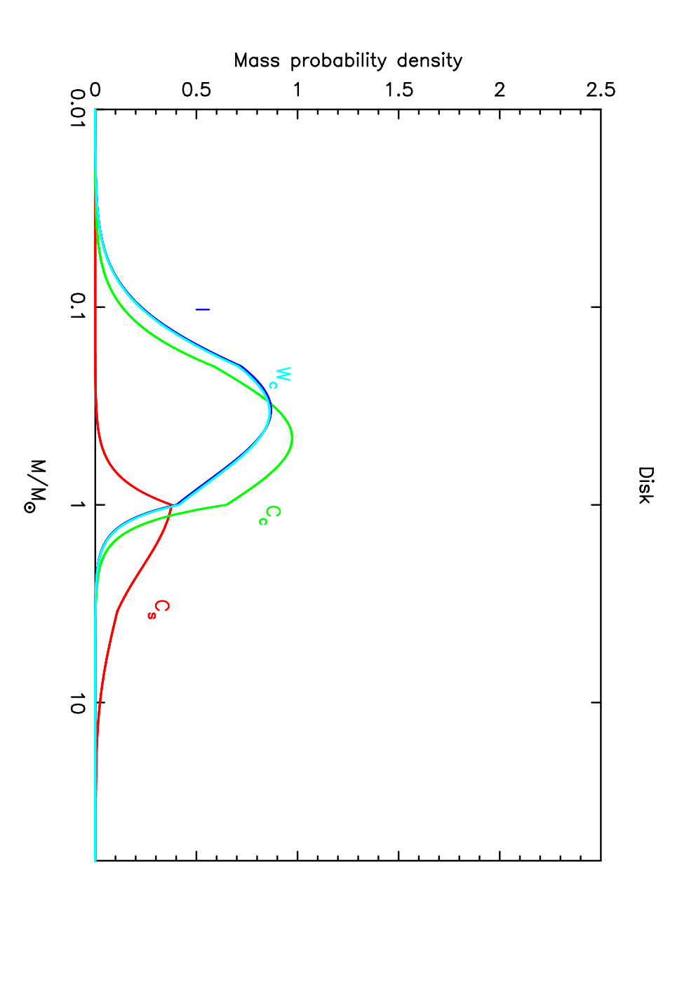

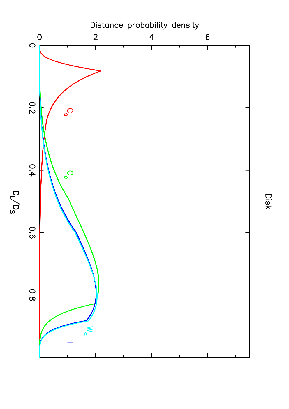

We use our fitted value of the source size parameter to place constraints on the mass of the lens, which can be expressed as a function of fractional distance and the source size as (e.g. Dominik 1998)
| (2) |
where is the mass of the lens, is the angular radius of the source, the value of which is given in Table 2, and other quantities are defined as before. The mass-distance curve showing constraints from this equation is plotted on Fig. 11.
However, since we cannot measure parallax for this event, we use a probabilistic approach following that of Dominik (2006) to derive probability densities for physical properties of lens components. The Galactic model used here is a piecewise mass spectrum (e.g. Chabrier 2003), two double exponentials for the disk mass density and a barred bulge tilted at an angle of with the direction to the Galactic centre (Dwek et al. 1995), and the distribution of effective transverse velocities used in Dominik (2006).
Using these galactic models, we infer properties for the lensing system, separating the cases where the lens is in the Galactic disk and in the Galactic bulge. For a lens in the disk, we find a primary mass and a secondary mass of , at a distance of kpc with a lens velocity of . For a lens in the bulge, we find a primary mass and a secondary mass of , at a distance of kpc with a lens velocity . These are the physical lens properties for the lowest- model (model ). The values of these physical parameters for the other models are given in Table 2. Probabilty densities of these properties for all models are plotted on Fig. 10.

3.7.3 Discussion
For our lowest- model, the parameters we find imply very unusual properties of the lensing system. As discussed in Sec. 3.4, the fact that we find these types of models is a consequence of the fitting approach we are taking. Traditional fitting methods would struggle to find these minima, since most of them require providing a starting point in parameter space. This is an issue when solely using an MCMC algorithm to fit microlensing events: although an MCMC run may be able to make its way through parameter space to find minima reasonably far away from its starting point, it is highly unlikely that a chain will be able to reach a minimum that has parameters different from the starting point by more than one order of magnitude. As we see from Fig. 4, there exist minima in many parts of parameter space, with values of that are different by almost two orders of magnitude. These parameters are non-intuitive, since they cannot be guessed only by looking at the lightcurve. As a result, it is improbable that this kind of parameters will be used as starting points for ”classic” fitting algorithms.
We solve this problem for the static binary-lens case by resorting to the method described in Sec. 2.2. Using this approach, we manage to systematically locate minima in parameter space. However, one then has to be careful with interpreting the significance of the obtained model parameters. The shape of probability densities shown in Fig. 10 for model indicates that our value of push the lens mass towards the end of the adopted mass spectrum in the Galactic model we have adopted. This results in the abrupt transients seen on Fig. 10. Similarly, the mass-distance curve for model on Fig. 11 shows that the mass of the lens increases very rapidly for lenses above kpc. These unusual curves are caused by a value of days. Models with days (corresponding to the low- minimum visible on Fig. 3 & 4) are obviously not acceptable, but how can we formally reject them? Finding these models from minima in the surface shows the limits of using as a strong criterion for favouring models. A solution to this would be to use prior distributions on as many of the parameters as we can. During the MCMC part of our fitting process, this would mean that we obtain posterior distributions that are different from the ones obtained without using prior distributions on the parameters, or, equivalently, assuming uniform priors for all parameters. Such priors can be obtained in various ways, such as looking at the distribution of timescales for past microlensing events or calculating these distributions from Galactic models (e.g. Dominik 2006), or by using luminosity functions of the Galactic bulge to find a prior for the blending factor (e.g. Holtzman et al. 1998). Such work requires careful consideration of which priors are most appropriate to use, and is beyond the scope of this paper. Using these priors in combination with our method to find minima will lead to more robust determination of minima by taking into account our knowledge of physical parameter distributions.
4 Summary and prospects
Our analysis of OGLE-2007-BLG-472 is a good illustration of the importance and power of using parameters that are related to actual observed features. Indeed, despite incomplete coverage of the caustic entry and high blending, a few crucial data points and an appropriate choice of non-standard parameters enable us to find several good binary-lens model fits to our data for this event by exploring the parameter space systematically. Some of the good fits that we identify have unphysical parameters, and we must then reject them. However using this parameterisation allows us to be certain that the parameter space has been thoroughly explored. We find four models with different parameters: two close binary models, one intermediate configuration, and a wide binary model. The lowest- model corresponds to a G dwarf star being lensed by a binary system with component masses (for the primary) and (for the secondary), which are compatible with our blending values. However it is obvious from physical parameter distributions that using as a sole criterion for determining the best model is insufficient, because it does not take into account our knowledge of the distributions of physical parameters.
Since the approach presented in this paper can form the basis for a systematic, wide ranging exploration of the parameter space to localise all possible models for a given data set, it is particularly relevant to current efforts to automatise real-time fitting of binary-lens events. This could prove useful to provide faster feedback on the events being observed and prioritise observing schedules, especially on robotic telescopes. Expanding robotic telescope networks controlled by automated intelligent algorithms are expected to play an increasingly important role in microlensing surveys in the coming years (e.g. Tsapras et al. 2008). Fitting methods such as the one described in this paper are essential for making sure any anomalies are interpreted correctly, and that minima are located in as large a part of parameter space as possible.
Acknowledgements
NK acknowledges STFC studentship PA/S/S/2006/04497 and an STFC travel grant covering his observing run at La Silla. We thank David Warren for financial support for the Mt Canopus Observatory. NK thanks Pascal Fouqué for organising a workshop in Toulouse in November 2007, and Joachim Wambsganss and Arnaud Cassan for their invitation to visit the Astronomisches Rechen-Institut in Heidelberg in April 2008. We would like to thank the anonymous referee for his helpful comments on the manuscript. We also thank the University of Tasmania for access to their TPAC supercomputer on which part of the calculations were carried out. PF expresses his gratitude to ESO for a two months invitation at Santiago headquarters, Chile in October and November 2008. The OGLE project is partially supported by the Polish MNiSW grant N20303032/4275.
References
- Bond et al. (2004) Bond I. A., et al., 2004, ApJ, 606, L155
- Bramich (2008) Bramich D. M., 2008, MNRAS, 386, L77
- Cassan (2008) Cassan A., 2008, A&A, 491, 587
- Cassan et al. (2004) Cassan A., et al., 2004, A&A, 419, L1
- Chabrier (2003) Chabrier G., 2003, PASP, 115, 763
- Charbonneau (1995) Charbonneau P., 1995, ApJS, 101, 309
- Dominik (1998) Dominik M., 1998, A&A, 330, 963
- Dominik (1999) —, 1999, A&A, 349, 108
- Dominik (2006) —, 2006, MNRAS, 367, 669
- Dominik (2007) —, 2007, MNRAS, 377, 1679
- Dwek et al. (1995) Dwek E., et al., 1995, ApJ, 445, 716
- Einstein (1936) Einstein A., 1936, Science, 84, 506
- Eisenhauer et al. (2005) Eisenhauer F., et al., 2005, ApJ, 628, 246
- Erdl & Schneider (1993) Erdl H., Schneider P., 1993, A&A, 268, 453
- Geweke (1992) Geweke J., 1992, Evaluating the Accuracy of Sampling-Based Approaches to the Calculation of Posterior Moments. Oxford University Press, pp. 169–193
- Ghosh et al. (2004) Ghosh H., et al., 2004, ApJ, 615, 450
- Griest & Safizadeh (1998) Griest K., Safizadeh N., 1998, ApJ, 500, 37
- Holtzman et al. (1998) Holtzman J. A., Watson A. M., Baum W. A., Grillmair C. J., Groth E. J., Light R. M., Lynds R., O’Neil Jr. E. J., 1998, AJ, 115, 1946
- Jaroszynski et al. (2006) Jaroszynski M., et al., 2006, Acta Astronomica, 56, 307
- Kervella & Fouqué (2008) Kervella P., Fouqué P., 2008, A&A, 491, 855
- Kubas et al. (2005) Kubas D., et al., 2005, A&A, 435, 941
- Mao & Paczyński (1991) Mao S., Paczyński B., 1991, ApJ, 374, L37
- Paczyński (1986) Paczyński B., 1986, ApJ, 304, 1
- Stanek & Garnavich (1998) Stanek K. Z., Garnavich P. M., 1998, ApJ, 503, L131+
- Tsapras et al. (2008) Tsapras Y., et al., 2008, ArXiv e-prints, 808
- Udalski (2003) Udalski A., 2003, Acta Astronomica, 53, 291