跳到论文正文
W Papers独立论文阅读器 arXiv:0901.1232 论文正文 计算阅读时间 · 0%
引用这篇论文根据当前论文元数据生成,正式投稿前建议核对。


License: arXiv.org perpetual non-exclusive license
arXiv:0901.1232v1 [hep-ph] 09 Jan 2009

Neutrino Models

and

Leptogenesis

Submitted in total fulfilment of the requirements of the degree of

Doctor of Philosophy

Sandy Sheung Che Law

School of Physics

The University of Melbourne

AUSTRALIA

December, 2008

Produced on archival quality paper

Abstract

Ne u t r i n o properties can play a crucial role in determining the matter-antimatter asymmetry of the universe if thermal leptogenesis is the correct solution to the baryogenesis problem. Owing to this, the study of neutrino models goes beyond the mere purpose of generating tiny neutrino masses, and it is natural to incorporate the puzzle of the cosmic baryon asymmetry. To this end, we have investigated several different extensions of the neutrino model based on the type I seesaw mechanism with particular emphasis on their leptogenesis implications.

In the first part of our work, we present a thorough analysis, in the leptogenesis context, of constrained neutrino models which have an abelian family symmetry and one extra Higgs singlet. The general result is that although these models contain less free parameters than the default type I seesaw setup, they do not hinder the possibility of successful leptogenesis in both the one-flavor approximation and when flavor effects are included. In fact, we have discovered that they do not modify or provide significant constraints on the typical leptogenesis scenario with hierarchical heavy right-handed neutrinos.

We then explore how the seesaw sector in neutrino mass models may be constrained through symmetries to be completely determined in terms of low-energy mass, mixing angle and C​PCP violating phase observables, with the subsequent aim to study their leptogenesis implications. The key ingredient in achieving this connection between the two distinct energy sectors is to simultaneously employ intra- and inter-flavor symmetries so that the neutrino Dirac mass matrix is only given in terms of the charged-lepton or quark mass matrices while all relevant diagonalization matrices can be fully predicted by the theory. We have built illustrative models to demonstrate this and shown that leptogenesis can succeed in small regions of parameter space for the case where the neutrino Dirac and up-quark mass matrix are identical. Also, it has been found that when the neutrino Dirac mass matrix is equal to its charged-lepton counterpart, TeV scale heavy neutrinos are possible although it is unlikely that they can be detected in colliders.

Finally, we present a new leptogenesis scenario, where the lepton asymmetry is generated by C​PCP violating decays of heavy right-handed neutrinos via electromagnetic dipole moment couplings to the ordinary light neutrinos. Akin to the usual scenario where the decays are mediated through Yukawa interactions, we have shown, by explicit calculations, that the desired asymmetry can be produced through the interference of the corresponding tree-level and one-loop decay amplitudes involving the effective dipole moment operators. Furthermore, we find that the relationship of the leptogenesis scale to the light neutrino masses is similar to that for the standard Yukawa-mediated mechanism.

Declaration

This is to certify that

  • (i)

    the thesis comprises only my original work towards the PhD except where indicated in the Preface,

  • (ii)

    due acknowledgement has been made in the text to all other material used,

  • (iii)

    the thesis is less than 100,000 words in length, exclusive of table, maps, bibliographies, appendices and footnotes.

.

Sandy S. C. Law

Date:     /     /     

Preface

The work presented here comprises of five main chapters (excluding auxiliary materials such as bibliography and appendices):
Chapter 1 is an original literature review on the various topics relating to neutrino properties, baryon asymmetry of the universe and thermal leptogenesis;
Chapter 2, 3 and 4 are based on the work presented in Publications 1, 3 and 2 (see page List of Publications) respectively. They were done in collaboration with N. F. Bell (Chapter 4), X. G. He (Chapter 3), B. J. Kayser (Chapter 4) and R. R. Volkas (Chapter 2 and 3). Most of the initial ideas for these investigations are due to N. F. Bell (Chapter 4) and R. R. Volkas (Chapter 2 and 3). But, all subsequent analyses and methods of presentation are my own work with the exceptions of Sec. 3.4.4 where X. G. He has made a significant contribution, and the proof in Sec. 4.3.1 which is due to B. J. Kayser;
Chapter 5 is the conclusion.

Acknowledgements

“I do physics not because it, as a subject, is simple, but because the spirit of physics, that turns the complicated and seemingly unrelated into something that can be described by a common set of rules, makes everything else looks simple.”

Of all the people I wish to thank, perhaps the most important on the list are my parents. Indeed, this journey did not begin four years ago when I entered graduate school; nor ten years ago when I became a freshman at the University of Melbourne; nor fifteen years ago when I touched down in Australia, but twenty-eight years ago when I was given a name which carries the meaning: “to ascertain knowledge and wisdom”. Although as this journey is coming to a close, it is unclear whether I have achieved what these words may entail, there is no doubt that my parents’ unyielding support has been present every bit of the way. So it is fitting that I thank them here first and foremost.

Needless to say, however, there are many others who have played a role (big or small) in helping me get over the line. Although I shall not be able to list them all here due to the limited space available, their contribution is very much appreciated and noted. But for those I shall acknowledge here, let me now mention them below.

It is very rare that a student can succeed without the guidance and endless source of ideas of his/her advisors. Thus, to get this far, I must thank my two advisors, Ray Volkas and Nicole Bell. Ray has been particularly influential not only because he is my primary thesis supervisor, but also because he taught us at the undergraduate level. The latter allowed me to find out what theoretical physics is all about, to know what a role model theorist is like, and above all, to make the easy decision to switch from mathematics to physics. The rest is history. Nicole entered the picture a bit later but the project she suggested formed a pivotal part of my candidature. It must be emphasized that because of them, I had the privilege to collaborate with outstanding scientists, Xiao-Gang He (NTU, Taiwan) and Boris Kayser (Fermilab, USA), to whom I thank very much also.

Next, I would like to thank some of my fellow graduate students in physics (past and present). First of all, Damien George for his numerous ‘‘lessons’’ in physics, mathematics and computing over the years (even before we embarked on this PhD path together under Ray), and for the countless discussions we had on miscellaneous topics that have made me a smarter/better person 11 1 It was during one such discussion when we accidentally discovered that there is a secret message contained in this thesis.. Secondly, Andrew Coulthurst, Catherine Low and Alison Demaria for being great officemates and mentors; and Kristian McDonald, Benedict Carson, Jason Doukas and Jared Cole (quantum computing) for being great mentors, as well as for all the interesting chats. Thirdly, special mentions are due to Paul Fraser (Nuclear/Condense matter theory), Thomas Jacques, Melissa Makin (and Melissa Wals, quantum computing), Swati Singh (astrophysics), Nadine Pesor, Jayne Thompson, Rhys Davies (now at Oxford) and David Curtin (now at Cornell).

Furthermore, it is a pleasure to thank Bruce H. J. McKellar (emeritus professor) for his expert help and advices; Norm Frankel and Girish Joshi for many interesting conversations; Geoffrey Taylor for being one of my supervisory panel member; Kamala Lekamge, the physics librarian, for countless assistances with the books and journals; Colin Entwisle (tutoring and lab admin) for making 1st year teaching manageable for graduate students like me; Geoff Shute (emeritus and 1st year lab guru) for the numerous conversations, innovative ideas and answering my dumb questions on undergraduate physics; and Wing Hin Lai, my uncle in Singapore, for his ongoing support.

Finally, I would like to thank some of my good friends who have played a part over the years in making who I am: Jeffrey K. C. Chan (grad student in computer science, Melb), Alex S. C. Leong (PhD in Elec. Eng., Melb), Siegfried S. F. Leung (grad student in chemistry and long time friend, Yale), Roy Whitby (teacher, mentor and friend who has been pivotal to many of my achievements), and last but not least Fido, the black Labrador, who reminded me during my 68 days “isolation” from the rest of the world in producing this that life is more than just a thesis.

Sandy S. C. Law
December 2008

List of Acronyms

BBN Big Bang Nucleosynthesis
BooNE Booster Neutrino Experiment
CKM Cabibbo-Kobayashi-Maskawa
CMB Cosmic Microwave Background
CUORE Cryogenic Underground Observatory for Rare Events
CUORICINO “small” CUORE (test bench for CUORE)
EMDM ElectroMagnetic Dipole Moment
GERDA GERmanium Detector Array
GNO Gallium Neutrino Observatory
GUTs Grand Unified Theories
IGEX International Germanium EXperiment
ILC International Linear Collider
IMB Irvine-Michigan-Brookhaven
K2K KEK to Super-K (Long Baseline Experiment)
Kamiokande Kamioka Nucleon Decay Experiment
KamLAND Kamioka Liquid scintillator AntiNeutrino Detector
KATRIN KArlsruhe TRItium Neutrino experiment
KEK Ko Enerugi Kasokuki Kenkyu Kiko
(High Energy Accelerator Research Organization, Tsukuba)
LH Left-Handed
LHC Large Hadron Collider
LHS Left Hand Side
LMA Large Mixing Angle (MSW solution)
LSND Liquid Scintillator Neutrino Detector
MiniBooNE (first phase of) BooNE
MINOS Main Injector Neutrino Oscillation Search
MSW Mikheyev-Smirnov-Wolfenstein
PMNS Pontecorvo-Maki-Nakagawa-Sakata
RH Right-Handed
RHS Right Hand Side
SAGE Soviet-American Gallium Experiment
SDSS Sloan Digital Sky Survey
SM Standard Model (of particle physics)
SNO Sudbury Neutrino Observatory
SUSY SUperSYmmetry
VEV Vacuum Expectation Value
WMAP Wilkinson Microwave Anisotropy Probe

Chapter 1 Introduction

Ou r quest to understand how the universe works at the most fundamental levels has been the impetus behind the constant experimental and theoretical efforts in various fields of physics. Over time, there have been many important breakthroughs, but just as many (if not more) puzzling questions remain. Amongst the most intriguing of these is the origin of matter— the substance which almost everything we see today is made of. Indeed, the standard hot Big Bang model does not discriminate between matter and antimatter as far as their primordial evolution is concerned. Therefore, in order to produce the abundance of matter we observe today, other mechanisms must have been at play in the early universe such that the expected catastrophic annihilation between matter and antimatter was avoided.

In the pursuit of a satisfactory answer for this phenomenon, it is immediately clear that high energy physics will play an essential role since the primordial environment created soon after the Big Bang was very hot and dense. But similar to its cosmological counterpart, the Standard Model of Particle Physics (denoted SM throughout) is incomplete despite the enormous success it has enjoyed over the past decades. The first evidence of physics beyond the SM is the observation of neutrino oscillations. Its utmost importance is certainly not restricted to within the realm of precision particle physics, and as we shall explain in the sections to come, far-reaching implications for the cosmological evolution of matter and antimatter can result in certain scenarios.

As a consequence of this potential connection, the studies of neutrino properties and interactions contain added significance. From the theoretical standpoint, this interplay will inevitably lead to constraints in neutrino model building. It is therefore the aim of this work to explore several classes of neutrino models and their possible implications for the origin of matter.

To elucidate all these ideas and build the background for the chapters to come, we begin by briefly reviewing the relevant topics on the theory of neutrinos and cosmic baryon asymmetry generation.

1.1  The phenomenon of neutrino oscillations

1.1.1 Experimental evidence

The first real indication of the neutrino oscillation phenomenon (i.e. neutrinos can change flavor as they propagate) emerged as early as 1967 when Davis and his collaborators conducted experiments to measure the electron neutrino flux produced from the Sun using a chlorine detector (νe+37\nu_{e}+{}^{37}Cl →\rightarrow e−+37e^{-}+{}^{37}Ar) in the Homestake mine (South Dakota) [1] and found that there was a noticeable deficit in the observed value compared to that predicted by the standard solar model [2]. But at that time the oscillation hypothesis was not taken seriously for it required a very large mixing angle to work, which seemed at odds with the tiny quark mixing. It was not until many years later (in the period 1989 to 1996) that Kamiokande (Kamioka Nucleon Decay Experiment, in Japan) provided new experimental data to strengthen the case for solar νe\nu_{e} disappearance. They employed water Cˇ\check{\rm C}erenkov techniques to investigate elastic scattering events (ν​e−→ν​e−)(\nu e^{-}\rightarrow\nu e^{-}) and discovered that the measured flux was only about 55% of the expected size [3, 4]. Later, in 2001, these findings were consolidated in the much larger 50,000 ton experiment of Super-Kamiokande (about 15 times bigger than Kamiokande) [5].

It should be noted that the Kamiokande experiments were only sensitive to the higher energy B8{}^{8}\text{B} solar neutrinos (above 5 MeV), in contrast to those targeted by Davis et al. which included lower energy Be7{}^{7}\text{Be} neutrinos. Hence, complementary experiments using radiochemical method with gallium (νe+71\nu_{e}+{}^{71}Ga →\rightarrow e−+71e^{-}+{}^{71}Ge) to target the lowest energy neutrinos from p+pp+p nuclear reaction (as well as Be7{}^{7}\text{Be} neutrinos) were conducted by the Gallex/GNO [6] and later the SAGE collaborations [7]. Both experiments detected a deficit in the solar neutrino flux, and importantly, their results were also consistent with the idea of matter enhanced neutrino oscillations [8].

Further improvement to the solar neutrino analysis was achieved when the SNO (Sudbury Neutrino Observatory, Canada) experiment managed to make reliable measurements of the total solar neutrino flux using a heavy water (D2​O\text{D}_{2}\text{O}) detector to look for both charged-current induced (νe+d→e−+p+p\nu_{e}+d\rightarrow e^{-}+p+p) and neutral-current induced (ν+d→ν+p+n\nu+d\rightarrow\nu+p+n) reactions [9], where dd denotes deuteron. This result provided conclusive evidence for solar neutrino oscillation and confirmed the hypothesis at a significant 3.3σ\sigma level. Other experiments such as KamLAND (in Japan), a long-baseline (source-detector distance ∼180\sim 180 km) reactor experiment [10] looking for disappearance of ν¯e\overline{\nu}_{e}, and Borexino (in Italy), a real time scintillator based Be7{}^{7}\text{Be} low energy neutrino experiment [11] also played an important role in authenticating the oscillation picture for solar neutrinos.

An independent set of (perhaps more) compelling experimental evidence for neutrino oscillations came from the studies of atmospheric neutrinos. When primary cosmic rays (usually high energy protons) collide with nuclei in the upper atmosphere, a shower of hadrons, mostly pions (and some kaons) are created. These pions then undergo a chain of reactions (e.g. π−→ν¯μ​μ−→ν¯μ​νμ​νe​e−\pi^{-}\rightarrow\overline{\nu}_{\mu}\,\mu^{-}\rightarrow\overline{\nu}_{\mu}\nu_{\mu}\nu_{e}\,e^{-}) producing muon and electron fluxes that can be measured. As early as the 1980s, two groups, the IMB (Irvine-Michigan-Brookhaven) collaboration [12] and Kamiokande [13] had found a significant deficit in the muon neutrino flux that was too big to be ascribed to statistical errors. This opened up the interpretation that νμ↔ντ\nu_{\mu}\leftrightarrow\nu_{\tau} oscillation might be at play. Motivated by their initial results, the Kamiokande group expanded their investigation, and in 1998, Super-Kamiokande reported a νμ\nu_{\mu}-νe\nu_{e} ratio and asymmetry in the zenith angle distribution of μ\mu-type events that were very much consistent with the atmospheric neutrino oscillation picture [14]. More recently, experiments with accelerator νμ\nu_{\mu}’s such as K2K in Japan [15] and MINOS in USA [16] have further confirmed this interpretation.

1.1.2 Theoretical formulation

The experimental observation that neutrinos can oscillate from one flavor to another as they propagate is the strongest indication (barring some by now strongly disfavored exotic possibilities) for nonzero neutrino masses and mixing. To see this, consider the case of three neutrino species. We define the neutrino weak eigenstate να\nu_{\alpha} with flavor α\alpha (where α=e,μ, or ​τ\alpha=e,\mu,\text{ or }\tau) such that it is produced in association with the charged antilepton ℓ¯α\overline{\ell}_{\alpha} in a tree-level interaction with the WW boson. These weak eigenstates are in general different from the neutrino mass eigenstates νi\nu_{i} (with i=1,2, and ​3i=1,2,\text{ and }3), each having a (rest) mass given by mim_{i}. One can relate the weak and mass eigenstates via a unitary transformation11 1 Unitarity will guarantee that charged-current interactions of να\nu_{\alpha} always produce a charged lepton with the same flavor α\alpha., and write να\nu_{\alpha} as a coherent superposition of the νi\nu_{i} fields:

|να⟩=∑iUα​i∗​|νi⟩,|\nu_{\alpha}\rangle=\sum_{i}\,U_{\alpha i}^{*}\,|\nu_{i}\rangle\;, (1.1)

where the nine quantities Uα​iU_{\alpha i} make up the unitary matrix of basis transformation. The meaning of leptonic mixing can therefore be understood as the fact that in a charged-current interaction, the neutrino mass eigenstate which accompanies the production of (or otherwise involves) ℓ¯α\overline{\ell}_{\alpha} may not always be the same νi\nu_{i}.

When we are working in the charged lepton mass eigenbasis, this unitary matrix is the leptonic mixing matrix, also known as the Pontecorvo-Maki-Nakagawa-Sakata (PMNS) matrix [17], which is often parametrized as

UPMNS=(c12​c13s12​c13s13​e−i​δ−s12​c23−c12​s23​s13​ei​δc12​c23−s12​s23​s13​ei​δs23​c13−s12​s23+c12​c23​s13​ei​δc12​s23+s12​c23​s13​ei​δ−c23​c13)​(ei​α1/2000ei​α2/20001),U_{\text{PMNS}}=\begin{pmatrix}c_{12}c_{13}&s_{12}c_{13}&s_{13}\,e^{-i\delta}\\ -s_{12}c_{23}-c_{12}s_{23}s_{13}\,e^{i\delta}&c_{12}c_{23}-s_{12}s_{23}s_{13}\,e^{i\delta}&s_{23}c_{13}\\ -s_{12}s_{23}+c_{12}c_{23}s_{13}\,e^{i\delta}&c_{12}s_{23}+s_{12}c_{23}s_{13}\,e^{i\delta}&-c_{23}c_{13}\end{pmatrix}\hskip-5.0pt\begin{pmatrix}e^{i\alpha_{1}/2}&0&0\\ 0&e^{i\alpha_{2}/2}&0\\ 0&0&1\end{pmatrix}, (1.2)

where sm​n=sin⁡θm​n,cm​n=cos⁡θm​ns_{mn}=\sin\theta_{mn},c_{mn}=\cos\theta_{mn}, δ\delta is the C​PCP violating Dirac phase, while α1\alpha_{1} and α2\alpha_{2} denote the two Majorana phases 22 2 Neutrinos can be Majorana particles..

To quantify the phenomenon of a neutrino changing from flavor-α\alpha to flavor-β\beta as it propagates in vacuum 33 3 In this discussion, we will ignore neutrino oscillations in matter (the MSW effect) [8]., we are interested in the probability with which this happens, i.e. Pr​(να→νβ)\text{Pr}\left(\nu_{\alpha}\rightarrow\nu_{\beta}\right), a quantity that depends on how the |να⟩|\nu_{\alpha}\rangle state in (1.1) evolves with time. Because να\nu_{\alpha} is a superposition of the mass eigenfields νi\nu_{i} whose quantum mechanical evolution may be different, we must solve each |νi​(t)⟩|\nu_{i}(t)\rangle state individually and then coherently sum them up. Working in the rest frame of νi\nu_{i}, the state vector at the proper time τi\tau_{i} will satisfy the Schrödinger equation:

i​∂∂τi​|νi​(τi)⟩=mi​|νi​(τi)⟩.i\,\frac{\partial}{\partial\tau_{i}}\;|\nu_{i}(\tau_{i})\rangle=m_{i}\,|\nu_{i}(\tau_{i})\rangle\;. (1.3)

The solution to Eq. (1.3) is simply given by:

|νi​(τi)⟩=e−i​mi​τi​|νi​(0)⟩,|\nu_{i}(\tau_{i})\rangle=e^{-i\,m_{i}\tau_{i}}|\nu_{i}(0)\rangle\;, (1.4)

where |νi​(0)⟩|\nu_{i}(0)\rangle is the original state before propagation. By Lorentz invariance, we can express mi​τim_{i}\tau_{i} in terms of laboratory variables:

mi​τi=Ei​t−|pi|​L,m_{i}\,\tau_{i}=E_{i}\,t-|p_{i}|\,L\;, (1.5)

where EiE_{i} and |pi||p_{i}| are respectively, the energy and momentum of the νi\nu_{i} component of the neutrino, while LL and tt are the source-detector distance and the time it takes to traverse LL, as measured in the lab-frame 44 4 In practice, tt is not measured.. For neutrino beams used in experiments, it can be shown that only components of the beam with the same energy will contribute coherently to the oscillation signal [18]. Therefore, we can replace EiE_{i} with EE, and momentum |pi||p_{i}| is now given by

|pi|=E2−mi2≃E−mi22​E,|p_{i}|=\sqrt{E^{2}-m_{i}^{2}}\;\simeq\;E-\frac{m_{i}^{2}}{2E}\;, (1.6)

where in the last step, we have assumed mi≪Em_{i}\ll E. With this approximation for |pi||p_{i}| and applying relation (1.5), solution (1.4) becomes

|νi​(t)⟩\displaystyle|\nu_{i}(t)\rangle ≃e−i⁡[E⁡(t−L)+mi2​L/2​E]​|νi​(0)⟩,\displaystyle\simeq e^{-i\,\left[E(t-L)+m_{i}^{2}L/2E\right]}\;|\nu_{i}(0)\rangle\;,
=e−i​E​(t−L)e−imi2L/2E|νi(0)⟩.\displaystyle=e^{-i\,E(t-L)}\,e^{-i\,m_{i}^{2}L/2E}\;|\nu_{i}(0)\rangle\;. (1.7)

Since the phase factor e−i​E​(t−L)e^{-i\,E(t-L)} is the same for all ii, it may be neglected in (1.7). Thus, the amplitude for a neutrino να\nu_{\alpha} of energy EE changing to νβ\nu_{\beta} after propagating a distance LL through vacuum is

⟨νβ|να⟩≃∑iUα​i∗e−imi2L/2EUβ​i.\langle\nu_{\beta}|\nu_{\alpha}\rangle\simeq\sum_{i}\,U_{\alpha i}^{*}\,e^{-i\,m_{i}^{2}L/2E}\,U_{\beta i}\;. (1.8)

Squaring (1.8) and after some algebra, we deduce the corresponding probability as:

Pr​(να→νβ)≡|⟨νβ|να⟩|2\displaystyle\text{Pr}(\nu_{\alpha}\rightarrow\nu_{\beta})\equiv|\langle\nu_{\beta}|\nu_{\alpha}\rangle|^{2} =δα​β−4​∑i>jRe​(Uα​i∗​Uβ​i​Uα​j​Uβ​j∗)​sin2⁡[Δ​mi​j2​L4​E]\displaystyle=\delta_{\alpha\beta}-4\,\sum_{i>j}\,\text{Re}\left(U_{\alpha i}^{*}U_{\beta i}U_{\alpha j}U_{\beta j}^{*}\right)\,\sin^{2}\left[\frac{\Delta m^{2}_{ij}\,L}{4E}\right]
+2∑i>jIm(Uα​i∗Uβ​iUα​jUβ​j∗)sin[Δ​mi​j2​L2​E],\displaystyle\qquad+2\,\sum_{i>j}\,\text{Im}\left(U_{\alpha i}^{*}U_{\beta i}U_{\alpha j}U_{\beta j}^{*}\right)\,\sin\left[\frac{\Delta m^{2}_{ij}\,L}{2E}\right]\;, (1.9)

where Δ​mi​j2≡mi2−mj2\Delta m^{2}_{ij}\equiv m_{i}^{2}-m_{j}^{2}.

From this result, it is quite clear that when all neutrino masses mim_{i}’s are zero (or nonzero but degenerate) and hence, the second and third term in Eq. (1.9) disappear, neutrino oscillation is not possible. By the same token, the observation that νe\nu_{e} and νμ\nu_{\mu} do change flavor during propagation implies that (at least two of) νi\nu_{i}’s must be massive.

1.1.3 Oscillation parameters

One can combine the plethora of neutrino oscillation data gathered to date from the various solar, atmospheric, reactor and accelerator experiments (see Sec. 1.1.1) 55 5 Here, we shall ignore the LSND anomaly [19] because an oscillation explanation has been ruled out by MiniBooNE [20]. and place constraints on the relevant parameters shown on the right-hand side (RHS) of Eq. (1.9). For the three-flavor neutrino oscillation picture and invoking the parametrisation of (1.2), one can see that variables that are potentially relevant in controlling the effects of oscillation are the three mixing angles (θ12,θ23\theta_{12},\theta_{23} and θ13\theta_{13}), the C​PCP violating Dirac phase (δ\delta), the two Majorana phases (α1\alpha_{1} and α2\alpha_{2}), and two squared-mass differences (e.g. Δ​m212\Delta m_{21}^{2} and Δ​m312\Delta m_{31}^{2}).

It turns out that oscillation probabilities are insensitive to the Majorana phases while the null result from the short-baseline (L∼1L\sim 1km) reactor experiment CHOOZ (in France) [21] 66 6 This experiment looked for the disappearance of ν¯e\overline{\nu}_{e} at E∼E\sim 3 GeV, which is sensitive to the large squared-mass gap Δ​m312\Delta m_{31}^{2}, thus allowing the properties of ν3\nu_{3} to be probed. suggests that θ13\theta_{13} must be quite small, consequently making the observation of the Dirac phase rather difficult. The reason for this latter point is that in (1.2), the Dirac phase always appears as the combination: sin⁡θ13​e−i​δ\sin\theta_{13}\,e^{-i\,\delta}, which means a sufficiently small θ13\theta_{13} can always mask any C​PCP violating effects 77 7 It must be emphasized that the choice of associating θ13\theta_{13} with δ\delta in the parametrization of (1.2) is not vital to our conclusion here. As long as there is at least one mixing angle which is very small, one can always re-phase the mixing matrix so that δ\delta is associated with the term containing the small angle. Our choice of parametrization is naturally motivated by the CHOOZ result which indicates a tiny θ13\theta_{13}..

Overall, neutrino experiments have so far determined that there are two large (θ12,θ23\theta_{12},\theta_{23}) and one small (θ13\theta_{13}) mixing angles 88 8 This is in stark contrast to the quark sector where the CKM matrix [22] has three small mixing angles., as well as, a “small” (Δ​msol2\Delta m_{\textrm{sol}}^{2}) and a “large” (Δ​matm2\Delta m_{\textrm{atm}}^{2}) squared-mass differences which drive the solar and atmospheric neutrino oscillations respectively. Because the sign of Δ​matm2\Delta m_{\textrm{atm}}^{2} is not known, two arrangements for the neutrino mass spectrum are possible: with normal hierarchy, we identify Δ​matm2≡Δ​m312>0\Delta m_{\textrm{atm}}^{2}\equiv\Delta m_{31}^{2}>0, which gives m1<m2<m3m_{1}<m_{2}<m_{3} with

m2=m12+Δ​msol2,m3=m12+Δ​matm2,m_{2}=\sqrt{m_{1}^{2}+\Delta m_{\textrm{sol}}^{2}}\;,\qquad m_{3}=\sqrt{m_{1}^{2}+\Delta m_{\textrm{atm}}^{2}}\;, (1.10)

and for inverted hierarchy, we take Δ​matm2≡Δ​m322<0\Delta m_{\textrm{atm}}^{2}\equiv\Delta m_{32}^{2}<0 instead, implying m3<m1<m2m_{3}<m_{1}<m_{2} with

m1=m32+Δ​matm2−Δ​msol2,m2=m12+Δ​msol2.m_{1}=\sqrt{m_{3}^{2}+\Delta m_{\textrm{atm}}^{2}-\Delta m_{\textrm{sol}}^{2}}\;,\qquad m_{2}=\sqrt{m_{1}^{2}+\Delta m_{\textrm{sol}}^{2}}\;. (1.11)

Note that in both cases, we have used Δ​msol2≡Δ​m212>0\Delta m_{\textrm{sol}}^{2}\equiv\Delta m_{21}^{2}>0 (as implied by the matter-affected solar neutrino oscillations). The best-fit values at 1​σ1\sigma error level for these neutrino oscillation parameters in the three-flavor framework are summarised as follows [23]:

sin2⁡θ12=0.304−0.016+0.022,sin2⁡θ23=0.50−0.06+0.07,sin2⁡θ13≤0.01−0.011+0.016,\displaystyle\sin^{2}\theta_{12}=0.304^{+0.022}_{-0.016}\;,\quad\sin^{2}\theta_{23}=0.50^{+0.07}_{-0.06}\;,\quad\sin^{2}\theta_{13}\leq 0.01^{+0.016}_{-0.011}\;, (1.12)
Δ​msol2=7.65−0.20+0.23×10⁻⁵​ eV2,|Δ​matm2|=2.40−0.11+0.12×10⁻³​ eV2.\displaystyle\Delta m_{\textrm{sol}}^{2}=7.65^{+0.23}_{-0.20}\times 10^{-5}\text{ eV}^{2}\;,\quad|\Delta m_{\textrm{atm}}^{2}|=2.40^{+0.12}_{-0.11}\times 10^{-3}\text{ eV}^{2}\;. (1.13)

In this work, we shall take these values as standard inputs for many of our analyses.

1.1.4 Tribimaximal mixing

An interesting observation from the best-fit parameter values shown in (1.12) is that θ23\theta_{23} and θ13\theta_{13} correspond to almost maximal and no mixing respectively. This prompts the question as to whether Nature selects these extreme values at random or there is a more profound reason. If one assumes that the maximal and no mixing is exact (i.e. θ23=π/4\theta_{23}=\pi/4 and θ13=0\theta_{13}=0), then up to the Majorana phases, the mixing matrix (1.2) becomes

UBL=(cos⁡θ12sin⁡θ120−sin⁡θ122cos⁡θ12212−sin⁡θ122cos⁡θ122−12),U_{\text{BL}}=\begin{pmatrix}\cos\theta_{12}&\sin\theta_{12}&0\\ -\frac{\sin\theta_{12}}{\sqrt{2}}&\frac{\cos\theta_{12}}{\sqrt{2}}&\frac{1}{\sqrt{2}}\\ -\frac{\sin\theta_{12}}{\sqrt{2}}&\frac{\cos\theta_{12}}{\sqrt{2}}&-\frac{1}{\sqrt{2}}\end{pmatrix}\;, (1.14)

which is often referred to as “bi-large” mixing. A particularly beautiful aspect of UBLU_{\text{BL}} is that any neutrino mass matrix in the flavor (i.e. weak interaction) basis which has a μ\mu-τ\tau symmetry 99 9 In other words, exchanging the μ\mu and τ\tau columns followed by the μ\mu and τ\tau rows will leave the mass matrix unchanged. can be diagonalised by it if one chooses θ12\theta_{12} carefully. Moreover, it can be shown that the specific value needed for θ12\theta_{12} to diagonalise these types of mass matrices is independent of the mass eigenvalues. This suggests that for certain neutrino mass matrix structures, mixing angles and masses are not necessarily interconnected even though both of them are related to the same source. In fact, this feature is quite common for mass matrices in models with an underlying flavor symmetry (or family symmetry 1010 10 We shall use both terms interchangeably through out this work.). The class of mass matrices which has a diagonalisation matrix that is independent of any of the parameters in the original matrix or its eigenvalues has been dubbed “form-diagonalisable” [24]. We shall make use of this idea quite often in our neutrino model building in the chapters to come.

Another important mixing structure which is related to UBLU_{\text{BL}} is the so-called “tribimaximal” mixing scheme [25]. Noting that the best-fit value for θ12\theta_{12} is very well approximated by the relation: sin2⁡θ12=1/3\sin^{2}\theta_{12}=1/3, we substitute it into UBLU_{\text{BL}} and the result is the tribimaximal mixing matrix 1111 11 Tri-maximal and bi-maximal mixing in the 2nd and 3rd columns respectively.:

UTB=(23130−161312−1613−12).U_{\text{TB}}=\begin{pmatrix}\sqrt{\frac{2}{3}}&\frac{1}{\sqrt{3}}&0\\ -\frac{1}{\sqrt{6}}&\frac{1}{\sqrt{3}}&\frac{1}{\sqrt{2}}\\ -\frac{1}{\sqrt{6}}&\frac{1}{\sqrt{3}}&-\frac{1}{\sqrt{2}}\end{pmatrix}\;. (1.15)

This neutrino mixing structure has attracted ample attention over the years with many model builders attempting to reconstruct it via symmetries and auxiliary fields. Most notable examples are models with discrete (e.g. A4,Δ27A_{4},\Delta_{27}) and continuous (e.g. S​O​(3),S​U​(3)SO(3),SU(3)) family symmetries. Some recent examples can be found in [26, 27]. It should be noted though that many of these are often quite intricate and require additional constraints or a non-trivial Higgs sector for them to be viable, further highlighting the difficulties in explaining the peculiar mixing pattern of neutrinos.

Nevertheless, the tribimaximal structure itself presents a relatively simple manifestation of the neutrino mixing matrix that is more or less consistent with current experimental bounds. In the light of this, it is theoretically appealing to take UTBU_{\text{TB}} (with or without the Majorana phases) as the starting point in any model building or analyses involving the neutrino mass matrix. Our work here in the future chapters will be no exception.

1.2  The case of massive neutrinos

1.2.1 Absolute scale for neutrino masses

Because oscillation experiments have strongly indicated that at least some neutrinos must be massive, it is natural to ask the scale at which these masses are situated. In the discussion of oscillation parameters in Sec. 1.1.3, we have learnt that those experiments can help us determine the splitting between the neutrino mass eigenstates, leading to Eqs. (1.10) and (1.11). However, it is clear that those relations do not tell us the overall scale of masses, and therefore other methods must be used to probe for a better understanding of the neutrino mass spectrum.

One way to obtain meaningful bounds on the absolute scale for the neutrinos is to look for kinematic effects due to their nonzero masses in tritium β\beta-decay (3H →He3+ν¯e+e−\rightarrow{}^{3}\text{He}+\overline{\nu}_{e}+e^{-}). By studying the resultant electron energy spectrum, one can probe the quantity:

mβ≡∑i=13|Ue​i|2​mi2.m_{\beta}\equiv\sqrt{\sum_{i=1}^{3}|U_{ei}|^{2}\,m_{i}^{2}}\;. (1.16)

The value of this then gives an upper limit on the absolute neutrino mass scale. Two groups, Mainz [28] and Troitsk [29], have reported bounds of mν<2.3m_{\nu}<2.3 eV and mν<2.5m_{\nu}<2.5 eV respectively. An upcoming experiment, KATRIN [30], is expected to have a sensitivity down to about 0.3 eV, which will further narrow down the scale of the neutrino spectrum. It should be remarked that whether neutrinos are of Dirac or Majorana type 1212 12 See the next two subsections for more discussions on Dirac and Majorana neutrinos. has no bearing on the capability of this method of “directly” searching for their masses.

Another possible way to probe the neutrino mass scale is via studies of lepton number (LL) violating neutrinoless double β\beta-decay ([Nucl]ZA→Z+2A[Nucl′]+2e−{}^{A}_{Z}\left[\text{Nucl}\right]\rightarrow\;^{\;\;\;\;A}_{Z+2}\left[\text{Nucl}^{\prime}\right]+2e^{-}), whose observation would imply that neutrinos are Majorana fermions [31]. Assuming that there are no new LL violating interactions at play, one can conclude that the amplitude for this decay is proportional to the so-called effective Majorana neutrino mass:

mβ​β≡|∑i=13Ue​i2​mi|.m_{\beta\beta}\equiv\left|\sum_{i=1}^{3}U_{ei}^{2}\,m_{i}\right|\;. (1.17)

Several groups such as the Heidelberg-Moscow [32] and IGEX [33] collaborations conducted experiments with Ge76{}^{76}\text{Ge}, while the more recent CUORICINO experiment [34] used Te130{}^{130}\text{Te} to test for this. So far there are no confirmed discoveries of the neutrinoless double β\beta-decay 1313 13 There is actually a claim by a subset of the Heidelberg-Moscow group that neutrinoless double β\beta-decay was observed [35]. For a more thorough discussion on this controversial finding, see [36]., but the best upper bounds on the decay lifetimes are presently provided by CUORICINO (which is still running), whose results are translated to 1414 14 The large range is due to the uncertainty in the nuclear matrix elements.

mν≡mβ​β<0.19−0.68​ eV ​(90%​ C.L.),m_{\nu}\equiv m_{\beta\beta}<0.19-0.68\text{ eV }\;(90\%\text{ C.L.})\;, (1.18)

for the neutrino mass. Relation (1.18) is a much tighter bound than the one obtained from tritium β\beta-decay. Upcoming experiments like CUORE [37], GERDA [38] and Majorana [39] are expected to further improve these results with projected sensitivity of about 0.05 eV.

Neutrino masses from cosmology

Finally, it must be mentioned that some of the strongest bounds on the overall scale for neutrino masses come from cosmology. This is one of the important examples that illustrates the intricate connections between neutrino physics and the evolution of the early universe. During the epoch of structure formation, free-streaming neutrinos with a sizable mass can have significant effects on the growth of structure and hence on the eventual galaxy power spectrum. Therefore, an accurate measurement of it can help set limits on the neutrino mass scale given the standard theory of structure formation. The studies of the data from the Wilkinson Microwave Anisotropy Probe (WMAP) and the Sloan Digital Sky Survey (SDSS) have deduced that the sum of neutrino masses (three species assumed) is constrained by ∑i|mi|≲0.6\sum_{i}\,|m_{i}|\lesssim 0.6 [40] and 1.61.6 eV [41] respectively at a confidence level of about 95%. Since the observed squared-mass splittings (Δ​msol2,Δ​matm2\Delta m_{\textrm{sol}}^{2},\Delta m_{\textrm{atm}}^{2}) imply that |mi−mj|≪𝒪⁡(0.1)|m_{i}-m_{j}|\ll\mathcal{O}\left(0.1\right) eV for all ii and jj, taking ∑i|mi|≲0.6\sum_{i}\,|m_{i}|\lesssim 0.6 gives an absolute upper bound for each individual neutrino mass of about

|mi|≲ 0.2​ eV ​(95%​ C.L.)for all ​i.|m_{i}|\;\lesssim\;0.2\text{ eV }\;\;(95\%\text{ C.L.})\quad\text{for all }i\;. (1.19)

This estimation is similar to the least upper bound imposed by the CUORICINO experiment, which further confirms that the absolute neutrino mass scale must be in the sub-eV range.

The immediate impact of these findings is that it raises the question as to why the neutrino is so light compared to other SM particles (e.g. mν/me∼10−6m_{\nu}/m_{e}\sim 10^{-6}), an issue we will return to in Secs. 1.2.3 to 1.2.5.

1.2.2 Neutrino mass terms

The minimal Standard Model (SM) does not include neutrino masses. But as we have discussed, the existence of massive neutrinos is the most natural explanation for the oscillation experiments. Therefore, it is imperative to modify the SM to include this fact. The only question is: how to do this?

Since only chirally left-handed (LH) fermion fields participate in weak interactions, it makes sense to express the SM fields in terms of their chiral components. To this end, we can define the following two-component Weyl spinors:

ψL,R≡PL,R​ψ=1∓γ52​ψ,\psi_{L,R}\equiv P_{L,R}\;\psi=\frac{1\mp\gamma^{5}}{2}\;\psi\;, (1.20)

where ψ\psi is a four-component Dirac spinor. Because a standard mass term for fermions has the form given by m​ψ¯​ψm\overline{\psi}\psi, when expressed in ψL,R\psi_{L,R} one finds that only fields of opposite chirality couple together. Consequently, two types of mass term are possible:

m𝒟​ψL¯​ψR+h.c.,m_{\mathcal{D}}\,\overline{\psi_{L}}\,\psi_{R}+\text{h.c.}\;, (1.21)

which is known as the Dirac mass term, and

Mℒ​ψL¯​(ψL)c+Mℛ​(ψR)c¯​ψR+h.c.,M_{\mathcal{L}}\,\overline{\psi_{L}}\,(\psi_{L})^{c}+M_{\mathcal{R}}\,\overline{(\psi_{R})^{c}}\,\psi_{R}+\text{h.c.}\;, (1.22)

which are called Majorana mass terms. The charge conjugate field is defined by ψc≡C​ψ¯T\psi^{c}\equiv C\,\overline{\psi}^{T} where CC denotes the charge conjugation matrix. These mass terms are so named because (1.21) arises from the coupling of Dirac type fields: ψ=ei​φ1​ψL+ei​φ2​ψR\psi=e^{i\varphi_{1}}\psi_{L}+e^{i\varphi_{2}}\psi_{R}, whereas the terms in (1.22) come from coupling of Majorana type fields: Ψa,b=ei​φ1​ψL,R+ei​φ2​(ψL,R)c\Psi_{a,b}=e^{i\varphi_{1}}\psi_{L,R}+e^{i\varphi_{2}}(\psi_{L,R})^{c}, which satisfy the Majorana condition:

(Ψa,b)c=e−i⁡(φ1+φ2)​Ψa,b,(\Psi_{a,b})^{c}=e^{-i\,(\varphi_{1}+\varphi_{2})}\,\Psi_{a,b}\;, (1.23)

where φ1,2\varphi_{1,2} are constants 1515 15 In (1.21) and (1.22), overall phases involving φ1,2\varphi_{1,2} are absorbed into the definitions of m𝒟m_{\mathcal{D}} and Mℒ,ℛM_{\mathcal{L},\mathcal{R}}.. The important implication of (1.23) is that Ψa,b\Psi_{a,b} are identical to their antiparticles.

At this point it is worth emphasizing that because of electric charge conservation, the existence of Majorana type masses for all charged fermions in the SM is forbidden. But since neutrinos are electrically neutral, all mass terms in (1.21) and (1.22) may be relevant, and as a result, one can have either massive Dirac or Majorana neutrinos.

For massive Dirac neutrinos, it is obvious from (1.21) that two different Weyl fields are required to construct the mass term. So, in addition to the νL\nu_{L} as seen in weak interactions, one must introduce a chirally right-handed (RH) neutrino field, νR\nu_{R}, to the SM. These RH neutrinos are weak isospin singlets and can therefore couple to the νL\nu_{L} and ϕ\phi, the SM Higgs doublet, to form the Yukawa term:

Yν​ℓ¯L​ϕ​νR+h.c.,Y_{\nu}\;\overline{\ell}_{L}\,\phi\,\nu_{R}+\text{h.c.}\;, (1.24)

where ℓL=(eL,νL)T\ell_{L}=(e_{L},\nu_{L})^{T} is a doublet of S​U​(2)LSU(2)_{L}. When the neutral component of the Higgs field ϕ\phi acquires a vacuum expectation value, (1.24) will induce a Dirac mass term for the neutrino. This is the same mechanism through which all quarks and charged leptons get their masses. However, in order to explain why neutrino is much lighter than other fermions, one has to impose a hierarchy in the Yukawas: Yν≪YeY_{\nu}\ll Y_{e}, making it seem rather ad-hoc. We shall discuss some possible resolutions to this later.

Turning to the case of massive Majorana neutrinos, it is clear from (1.22) that only one type of Weyl field is required in principle. Hence, given νL\nu_{L}, one can already construct a Majorana mass term for the neutrino. But since ℓ¯L​ℓLc\overline{\ell}_{L}\,\ell_{L}^{c} is a weak isospin triplet, within the framework of the SM, the simplest possibility is therefore the dimension-5 mass term of the form [42]:

y2Λ​ℓ¯L​ϕ​ϕT​ℓLc+h.c.,\frac{y^{2}}{\Lambda}\,\overline{\ell}_{L}\,\phi\,\phi^{T}\ell_{L}^{c}+\text{h.c.}\;, (1.25)

where yy denotes some dimensionless coupling constant and Λ\Lambda is the high-energy cutoff scale above which this non-renormalisable interaction is no longer valid. After spontaneous symmetry breaking, the term in (1.25) will induce an effective Majorana mass for the neutrino:

mν=y2​⟨ϕ0⟩2Λ.m_{\nu}=\frac{y^{2}\langle\phi^{0}\rangle^{2}}{\Lambda}\;. (1.26)

It is interesting to note here that if Λ≫⟨ϕ0⟩\Lambda\gg\langle\phi^{0}\rangle, then expression (1.26) suggests that neutrinos can naturally have a much smaller mass than other fermions without the need to fine-tune yy with the corresponding Yukawa coupling of the charged leptons. Given this potential benefit in models with Majorana neutrino masses, and the fact that no SM symmetry forbids their inclusion, it seems natural that neutrinos ought to be Majorana particles. Consequently, we shall assume throughout this work that neutrinos are Majorana unless otherwise indicated.

Returning to the initial problem of how to modify the SM to incorporate neutrino masses, we see that both the Dirac mass term of (1.24) and the non-renormalisable term of (1.25) imply that some new physics must be introduced. While (1.24) demands the addition of RH singlet neutrinos, (1.25) can lead to many possibilities. So, it is the subject of the next few subsections to explore several possible scenarios which can achieve this within framework of renormalisable interactions.

1.2.3 Seesaw mechanism: type I

Within the class of renormalisable models that can give rise to the effective interaction of form (1.25), the type I seesaw mechanism [43] is perhaps the most elegant solution of all. Not only can it provide a way to generate tiny but nonzero neutrino masses, it also contains all the necessary ingredients for explaining the cosmic baryon asymmetry, as will be discussed in more detail later in Sec. 1.4.

The idea of the type I seesaw model is quite simple. It springs from the inclusion of heavy neutral singlet fermions, the RH neutrinos (one for each generation of light neutrino) in the SM, just as one would require to have a Dirac neutrino mass term. But since the RH neutrinos are electroweak singlets, one can also include a Majorana mass term for them. As a result of having both Dirac and Majorana mass terms, one gets the following Lagrangian which is SM gauge invariant:

−ℒtype-I=Yν​ℓ¯L​ϕ​νR+MR2​(νR)c¯​νR+h.c.,-\mathcal{L}_{\text{type-I}}=Y_{\nu}\,\overline{\ell}_{L}\,\phi\,\nu_{R}+\frac{M_{R}}{2}\,\overline{(\nu_{R})^{c}}\,\nu_{R}+\text{h.c.}\;, (1.27)

where MRM_{R} denotes the bare mass for the RH neutrino. Since the SM does not predict or restrict the size of MRM_{R}, we may assume that it is arbitrarily large. So, by integrating out the heavy RH neutrino field, one gets an effective Lagrangian that is of the same form as (1.25):

ℒeffI=Yν22​MR​ℓ¯L​ϕ​ϕT​ℓLc,\mathcal{L}_{\text{eff}}^{\rm I}=\frac{Y_{\nu}^{2}}{2M_{R}}\,\overline{\ell}_{L}\,\phi\,\phi^{T}\ell_{L}^{c}\;, (1.28)

if we identify yy and Λ\Lambda of Eq. (1.25) with YνY_{\nu} and MRM_{R} respectively. The interaction of (1.28) will naturally give rise to a very small Majorana neutrino mass: mν≃⟨ϕ0⟩2​Yν​MR−1​YνTm_{\nu}\simeq\langle\phi^{0}\rangle^{2}\,Y_{\nu}\,M_{R}^{-1}\,Y_{\nu}^{T} if one assumes that MR≫⟨ϕ⟩M_{R}\gg\langle\phi\rangle. This situation is illustrated in Fig. 1.1.

Refer to caption
Figure 1.1: Diagram representing the type I seesaw realisation of the small Majorana mass for the LH neutrino with mν≃⟨ϕ0⟩2​Yν​MR−1​YνTm_{\nu}\simeq\langle\phi^{0}\rangle^{2}\,Y_{\nu}\,M_{R}^{-1}\,Y_{\nu}^{T} (up to a multiplicative constant).

Equivalently, one can obtain this by writing (1.27) in matrix form and subsequently block-diagonalising the resultant 2​n×2​n2n\times 2n neutrino matrix, where nn is the number of generations. To elucidate this, we begin by rewriting the Lagrangian (1.27) in index form with the generation indices i,ji,j included (ignoring the charged lepton terms):

−2​ℒν=∑i,jnν¯i​L​(mD)i​j​νj​R+(νj​R)c¯​(mD)j​i​νi​Lc+(νR​i)c¯​(MR)i​j​νj​R+h.c.,-2\mathcal{L}_{\nu}=\sum_{i,j}^{n}\,\overline{\nu}_{iL}\,(m_{D})_{ij}\,\nu_{jR}+\overline{(\nu_{jR})^{c}}\,(m_{D})_{ji}\,\nu_{iL}^{c}+\overline{(\nu_{Ri})^{c}}\,(M_{R})_{ij}\,\nu_{jR}+\text{h.c.}\;, (1.29)

where mD≡Yν​⟨ϕ0⟩m_{D}\equiv Y_{\nu}\langle\phi^{0}\rangle and we have used the fact: νL¯​νR≡(νR)c¯​(νL)c\overline{\nu_{L}}\nu_{R}\equiv\overline{(\nu_{R})^{c}}(\nu_{L})^{c}. Then, (1.29) can be re-packaged into:

−2​ℒν=(ν¯L(νR)c¯)​(0mDmDTMR)⏟M​((νL)cνR)+h.c.,-2\mathcal{L}_{\nu}=\begin{pmatrix}\overline{\nu}_{L}&\overline{(\nu_{R})^{c}}\end{pmatrix}\underbrace{\begin{pmatrix}0&m_{D}\\ m_{D}^{T}&M_{R}\\ \end{pmatrix}}_{M}\begin{pmatrix}(\nu_{L})^{c}\\ \nu_{R}\end{pmatrix}+\text{h.c.}\;, (1.30)

where νL≡(ν1​L,…,νn​L)T\nu_{L}\equiv(\nu_{1L},\ldots,\nu_{nL})^{T} and νR≡(ν1​R,…,νn​R)T\nu_{R}\equiv(\nu_{1R},\ldots,\nu_{nR})^{T}. Using the key assumption that all eigenvalues of mDm_{D} are much less than those of MRM_{R}, the neutrino mass matrix in (1.30) may be block-diagonalised (to first order in MR−1​mDTM_{R}^{-1}m_{D}^{T}) by:

Dν\displaystyle D_{\nu} =V​M​VT,\displaystyle=V\,M\,V^{T}\;,
≃(mD​MR−1​mDT00MR),\displaystyle\simeq\begin{pmatrix}m_{D}\,M_{R}^{-1}\,m_{D}^{T}&0\\ 0&M_{R}\\ \end{pmatrix}\;, (1.31)
where
V\displaystyle V =(I(MR−1​mDT)†−MR−1​mDTI)​(i​I00I).\displaystyle=\begin{pmatrix}I&(M_{R}^{-1}\,m_{D}^{T})^{\dagger}\\ -M_{R}^{-1}\,m_{D}^{T}&I\\ \end{pmatrix}\begin{pmatrix}i\,I&0\\ 0&I\\ \end{pmatrix}\;. (1.32)

The second matrix in the definition of (1.32) is included to ensure all mass eigenvalues are positive. If we let (ν′,N′)T=(νL,νRc)T​VT(\nu^{\prime},N^{\prime})^{T}=(\nu_{L},\nu_{R}^{c})^{T}V^{T} and define a set of Majorana fields:

(νN)≡(ν′+(ν′)cN′+(N′)c),\begin{pmatrix}\nu\\ N\end{pmatrix}\equiv\begin{pmatrix}\nu^{\prime}+(\nu^{\prime})^{c}\\ N^{\prime}+(N^{\prime})^{c}\end{pmatrix}\;, (1.33)

then Lagrangian (1.30) becomes

−2​ℒν\displaystyle-2\mathcal{L}_{\nu} =(mD​MR−1​mDT)​ν¯​ν+MR​N¯​N+h.c.,\displaystyle=(m_{D}\,M_{R}^{-1}\,m_{D}^{T})\,\overline{\nu}\,\nu+M_{R}\,\overline{N}\,N+\text{h.c.}\;,
=mν​ν¯​ν+MR​N¯​N+h.c..\displaystyle=m_{\nu}\,\overline{\nu}\,\nu+M_{R}\,\overline{N}\,N+\text{h.c.}\;. (1.34)

So from this, it is easy to see that this model gives rise to two sets of Majorana neutrinos: the light ones (ν\nu) with mass matrix mν≃mD​MR−1​mDT≡⟨ϕ0⟩2​Yν​MR−1​YνTm_{\nu}\simeq m_{D}\,M_{R}^{-1}\,m_{D}^{T}\equiv\langle\phi^{0}\rangle^{2}\,Y_{\nu}\,M_{R}^{-1}\,Y_{\nu}^{T}, and the heavy ones (NN) with MN≃MRM_{N}\simeq M_{R}. A particularly attractive feature of this is that the smallness of mνm_{\nu} is a direct consequence of the large mass scale of MRM_{R}, which may have its origin from higher unification theories. Furthermore, the addition of RH neutrinos per se seems quite natural from the point of view of making the SM more “left-right” (and “quark-lepton”) symmetric, in the sense that for each LH fermion, there is a RH version. Owing to these benefits, the type I seesaw framework will form the central theme of all of our subsequent investigations in this present work.

1.2.4 Other seesaw models

Besides type I seesaw, there exist other extensions to the SM which can lead to the effective Majorana mass term in (1.25). These seesaw-like models provide alternative ways to understand the smallness of neutrino mass [44], and hence are of great interest to many model builders 1616 16 Small neutrino masses can also be generated without seesaw in models with extra dimensions [45].. So, for completeness, we will briefly review them here despite the fact that they play no direct role in our current work.

Type II seesaw

Instead of extending the SM by adding heavy singlet fermions as in Sec. 1.2.3, one can make use of the fact that ℓ¯L​ℓLc\overline{\ell}_{L}\,\ell_{L}^{c} is an S​U​(2)LSU(2)_{L} triplet and introduce a heavy triplet scalar to the Higgs sector [46], so that a gauge invariant and renormalisable ℓ¯L​ℓLc\overline{\ell}_{L}\,\ell_{L}^{c}-type mass term can be formed. Specifically, suppose we have a heavy S​U​(2)LSU(2)_{L} triplet scalar field Δ\Delta with hypercharge Y=−2Y=-2 and a convenient 2×22\times 2 matrix parametrization given by

Δ=(Δ−/2Δ−⁣−Δ0−Δ−/2),\Delta=\begin{pmatrix}\Delta^{-}/\sqrt{2}&\Delta^{--}\\ \Delta^{0}&-\Delta^{-}/\sqrt{2}\\ \end{pmatrix}\;, (1.35)

then the Lagrangian

−ℒtype-II=YΔ2​ℓ¯L​i​τ2​Δ​ℓLc+μΔ​ϕT​Δ​ϕ+MΔ2​Δ†​Δ+h.c.,-\mathcal{L}_{\text{type-II}}=\frac{Y_{\Delta}}{2}\,\overline{\ell}_{L}i\tau_{2}\,\Delta\,\ell_{L}^{c}+\mu_{\Delta}\,\phi^{T}\Delta\,\phi+M_{\Delta}^{2}\,\Delta^{\dagger}\Delta+\text{h.c.}\;, (1.36)

will give rise to the process depicted in Fig. 1.2a. This then leads to an effective mass term

meffII\displaystyle m_{\text{eff}}^{\rm II} ≃μΔ​YΔ​⟨ϕ0⟩2MΔ2,\displaystyle\simeq\,\mu_{\Delta}\,Y_{\Delta}\frac{\langle\phi^{0}\rangle^{2}}{M_{\Delta}^{2}}\;,
=λΔ​YΔ​⟨ϕ0⟩2MΔ, after setting ​μΔ≡λΔ​MΔ.\displaystyle=\,\lambda_{\Delta}\,Y_{\Delta}\frac{\langle\phi^{0}\rangle^{2}}{M_{\Delta}}\;,\quad\text{ after setting }\;\;\mu_{\Delta}\equiv\lambda_{\Delta}M_{\Delta}\;. (1.37)

This expression has the same form as (1.26) with the couplings λΔ​YΔ\lambda_{\Delta}Y_{\Delta} playing the role of y2y^{2}. So, when MΔ≫⟨ϕ0⟩M_{\Delta}\gg\langle\phi^{0}\rangle, small neutrino masses can be induced. This mechanism is known as type II seesaw [46].

Refer to caption
Figure 1.2: (a) The process induced by the type II seesaw Lagrangian that will give rise to small neutrino Majorana masses. (b) The corresponding process in the type III seesaw case with heavy triplet fermion Σ\Sigma instead.
Type III seesaw

Another possibility is to replace the RH neutrinos with heavy triplet fermions and allow them to interact with the ordinary lepton doublets via Yukawa couplings [47]. In this scenario, the Higgs sector is unmodified, and a set of self-conjugate S​U​(2)LSU(2)_{L} triplets of exotic leptons with hypercharge Y=0Y=0 are added:

Σ=(Σ−Σ0/2Σ0/2Σ+).\Sigma=\begin{pmatrix}\Sigma^{-}&\Sigma^{0}/\sqrt{2}\\ \Sigma^{0}/\sqrt{2}&\Sigma^{+}\\ \end{pmatrix}\;. (1.38)

The corresponding Lagrangian for this model is given by

−ℒtype-III=YΣ​ℓ¯L​i​τ2​Σ​ϕ+MΣ​Tr​(Σc¯​Σ)+h.c.,-\mathcal{L}_{\text{type-III}}=Y_{\Sigma}\,\overline{\ell}_{L}\,i\tau_{2}\,\Sigma\,\phi+M_{\Sigma}\,\text{Tr}\left(\overline{\Sigma^{c}}\,\Sigma\right)+\text{h.c.}\;, (1.39)

This gives rise to the diagram shown in Fig. 1.2b, and after integrating out the heavy Σ\Sigma field, one obtains the desired form for the seesaw neutrino mass

meffIII≃YΣ​⟨ϕ0⟩2MΣ​YΣT.m_{\text{eff}}^{\rm III}\simeq\,Y_{\Sigma}\,\frac{\langle\phi^{0}\rangle^{2}}{M_{\Sigma}}\,Y_{\Sigma}^{T}\;. (1.40)

Hence by setting MΣ≫⟨ϕ0⟩M_{\Sigma}\gg\langle\phi^{0}\rangle, one can explain the smallness of neutrino masses, and as a result, this is often referred to as the type III seesaw mechanism [47].

1.2.5 Neutrino mass from radiative corrections

Finally, it should be mentioned that neutrino masses can also be induced from radiative corrections. Typically, this involves the enlargement of the Higgs sector and having the newly introduced charged scalars coupling to the LH lepton doublets, so that interactions of the form of (1.25) are created at loop level.

Zee model

One realisation of this concept is the so-called Zee model [48]. In this particular extension to the SM, there are two (or more) S​U​(2)LSU(2)_{L} Higgs doublets, all with the same hypercharge (Y⁡(ϕ)=1Y(\phi)=1) and a charged scalar singlet h−h^{-} which has Y⁡(h−)=−2Y(h^{-})=-2. With these, the scalar field h−h^{-} can couple to the LH lepton doublets in the following way:

ℒyukZ=κ​ϵi​j​ℓ¯Li​(ℓLj)c​h−+h.c.,\mathcal{L}_{\text{yuk}}^{\text{Z}}=\kappa\,\epsilon_{ij}\,\overline{\ell}_{L}^{i}\,(\ell_{L}^{j})^{c}\,h^{-}+\text{h.c.}\;, (1.41)

where i,ji,j are indices in S​U​(2)LSU(2)_{L} and ϵi​j\epsilon_{ij} denotes the Levi-Civita tensor. Furthermore, in the Higgs potential, one gets a cubic coupling term between h−h^{-} and other doublets in the model:

ℒcubicZ=μa​b​ϵi​j​ϕai​ϕbj​h−+h.c.,\mathcal{L}_{\text{cubic}}^{\text{Z}}=\mu_{ab}\,\epsilon_{ij}\,\phi_{a}^{i}\,\phi_{b}^{j}\,h^{-}+\text{h.c.}\;, (1.42)

where a,b=1,2,…a,b=1,2,\ldots are labels for the different Higgs doublets. When combining the tree-level interactions of (1.41), (1.42) and the standard Higgs Yukawa (ℓ¯L​ϕa,b​eR\overline{\ell}_{L}\,\phi_{a,b}\,e_{R}) together, a Majorana neutrino mass term of the form of (1.25) is induced via the one-loop diagram shown in Fig. 1.3a. Tiny neutrino masses can then be realised by carefully choosing the scale of the Higgses and assuming a small coupling for κ\kappa.

Refer to caption
Figure 1.3: (a) One-loop correction graph of the Zee model that generates a neutrino Majorana mass. (b) Two-loop diagram of the Babu-Zee model that contributes to the neutrino Majorana mass term.
Babu-Zee model

Another example of neutrino masses generated from radiative corrections is the so-called Babu-Zee model [49, 50]. In contrast to the Zee setup, it contains two charged scalar singlets: one singly charged (h−h^{-}) and the other doubly charged (k+⁣+k^{++}), together with only one Higgs doublet (the SM Higgs). The relevant interaction Lagrangian is then given by:

ℒintBZ=κ​ϵi​j​ℓ¯Li​(ℓLj)c​h−+λ​(eR)c¯​eR​k+⁣++μ​k+⁣+​h−​h−+Ye​ℓ¯L​ϕ​eR+h.c.,\mathcal{L}_{\text{int}}^{\text{BZ}}=\kappa\,\epsilon_{ij}\,\overline{\ell}_{L}^{i}\,(\ell_{L}^{j})^{c}\,h^{-}+\lambda\,\overline{(e_{R})^{c}}\,e_{R}\,k^{++}+\mu\,k^{++}\,h^{-}\,h^{-}+Y_{e}\,\overline{\ell}_{L}\,\phi\,e_{R}+\text{h.c.}\;, (1.43)

where κ,λ\kappa,\lambda and YeY_{e} are dimensionless coupling constants while constant μ\mu has a dimension of mass. These interactions can give rise to Majorana neutrino masses at the two-loop level as indicated in Fig. 1.3b.

1.2.6 Neutrino electromagnetic dipole moments

One of the important implications of massive neutrinos is that they can in general possess a nonzero transition magnetic and electric dipole moment (both for Dirac and Majorana neutrinos), regardless of the mechanism by which they gain their mass. If neutrinos are Dirac particles, then they can also have diagonal electromagnetic dipole moments [51, 52, 53, 54], unlike their Majorana counterparts. We can see this by first noting that the electromagnetic current that corresponds to magnetic and electric dipole moment interactions between two neutrinos has the form:

⟨νj​(p′)|Jμdm|νk​(p)⟩=ν¯j​[F⁡(q2)+i​γ5​G​(q2)]​σμ​ν​qν​νk,\langle\nu_{j}(p^{\prime})|J_{\mu}^{\text{dm}}|\nu_{k}(p)\rangle=\overline{\nu}_{j}\left[F(q^{2})+i\gamma^{5}G(q^{2})\right]\sigma_{\mu\nu}\,q^{\nu}\nu_{k}\;, (1.44)

where q=p′−pq=p^{\prime}-p, while F⁡(q2)F(q^{2}) and G⁡(q2)G(q^{2}) are the magnetic and electric dipole form factors respectively. For a Majorana field Ψ\Psi and j=kj=k (the diagonal case), Eq. (1.44) becomes

Ψ¯​[F+i​γ5​G]​σμ​ν​qν​Ψ\displaystyle\overline{\Psi}\left[F+i\gamma^{5}G\right]\sigma_{\mu\nu}\,q^{\nu}\Psi ≡(Ψ¯​[F+i​γ5​G]​σμ​ν​qν​Ψ)T,\displaystyle\equiv\left(\overline{\Psi}\left[F+i\gamma^{5}G\right]\sigma_{\mu\nu}\,q^{\nu}\Psi\right)^{T}\;, (1.45)
=−ΨT​[F+i​γ5​G]T​(σμ​ν)T​qν​Ψ¯T,\displaystyle=-\Psi^{T}\left[F+i\gamma^{5}G\right]^{T}(\sigma_{\mu\nu})^{T}q^{\nu}\,\overline{\Psi}^{T}\;, (1.46)

where the negative sign in (1.46) comes from anticommuting fermion fields and we have used the fact that γ5​σμ​ν=σμ​ν​γ5\gamma^{5}\sigma_{\mu\nu}=\sigma_{\mu\nu}\gamma^{5}. Using the following conventions for charge conjugation

ψc=C​ψ¯T,C†​γ5​C=(γ5)T,C†​σμ​ν​C=(−σμ​ν)T,\psi^{c}=C\overline{\psi}^{T}\;,\quad C^{\dagger}\gamma^{5}C=(\gamma^{5})^{T}\;,\quad C^{\dagger}\sigma_{\mu\nu}C=(-\sigma_{\mu\nu})^{T}\;,\quad (1.47)

expression (1.46) can be rewritten as

−ΨT​C†​[F+i​γ5​G]​(−σμ​ν)​qν​C​Ψ¯T,\displaystyle-\Psi^{T}C^{\dagger}\left[F+i\gamma^{5}G\right](-\sigma_{\mu\nu})q^{\nu}\,C\overline{\Psi}^{T}\;, (1.48)
=\displaystyle= −Ψc¯​[F+i​γ5​G]​σμ​ν​qν​Ψc,\displaystyle-\overline{\Psi^{c}}\left[F+i\gamma^{5}G\right]\sigma_{\mu\nu}q^{\nu}\Psi^{c}\;, (1.49)
=\displaystyle= −Ψ¯​[F+i​γ5​G]​σμ​ν​qν​Ψ,\displaystyle-\overline{\Psi}\left[F+i\gamma^{5}G\right]\sigma_{\mu\nu}q^{\nu}\Psi\;, (1.50)

where we have used the Majorana condition Ψc=ei​φ​Ψ\Psi^{c}=e^{i\varphi}\Psi. So, combining LHS of (1.45) and (1.50) implies that FF and GG must vanish. In other words, Majorana neutrinos cannot have diagonal dipole moments although they may possess transition moments.

To understand the connection between neutrino mass and neutrino dipole moment, one can compare the Feynman graphs which correspond to the generic contributions of these quantities as depicted in Fig. 1.4. By applying simple dimensional analysis on a generic dipole moment operator:

ℒdm=ν¯j​(μj​k+i​γ5​dj​k)​σα​β​νk​Fα​β,\mathcal{L}^{\text{dm}}=\overline{\nu}_{j}\,(\mu_{jk}+i\gamma^{5}d_{jk})\,\sigma_{\alpha\beta}\,\nu_{k}\,F^{\alpha\beta}\;, (1.51)

where Fα​βF^{\alpha\beta} denotes the photon field tensor, we see that the magnetic (μj​k\mu_{jk}) and electric (dj​kd_{jk}) dipole moments have dimension of inverse mass. Therefore, the contribution from the dipole moment interaction as shown in Fig. 1.4a can be expressed as

μν∼e​𝒢Λ,\mu_{\nu}\sim\frac{e\,\mathcal{G}}{\Lambda}\;, (1.52)

where ee is the coupling from the photon vertex, 𝒢\mathcal{G} denotes the combination of dimensionless parameters such as coupling constants (except ee), mass ratios, mixing angles and 1/16​π21/16\pi^{2} loop factors which may appear in the graph, while Λ\Lambda is some energy scale beyond the SM at which the dipole moment is generated. Similar analysis for Fig. 1.4b where the external photon line has been removed gives a radiative correction to the neutrino mass of order

mν∼𝒢​Λ.m_{\nu}\sim\mathcal{G}\,\Lambda\;. (1.53)

Therefore, putting (1.52) and (1.53) together, a simple relationship between neutrino mass and dipole moment can be obtained:

μν∼e​mνΛ2≃10−18​(mν1​ eV)​(1​ TeVΛ)2​μB,\mu_{\nu}\sim\frac{e\,m_{\nu}}{\Lambda^{2}}\simeq 10^{-18}\left(\frac{\phantom{I}m_{\nu}\phantom{I}}{1\text{ eV}}\right)\left(\frac{1\text{ TeV}}{\Lambda}\right)^{2}\mu_{B}\;, (1.54)

where μB=e/2​me\mu_{B}=e/2m_{e} is the Bohr magneton.

Refer to caption
Figure 1.4: (a) A generic Feynman graph representing the contribution to neutrino electromagnetic dipole moments. (b) The corresponding graph with the photon line removed which gives a radiative contribution to neutrino mass. The shaded blob denotes some new physics beyond the SM which gives rise to the neutrino dipole moments and/or masses.

Although, in a more general context, where new symmetries or physics are employed [55, 56], zero neutrino masses do not necessarily imply vanishing dipole moments, the case of massive neutrinos, however, naturally allows for dipole moments to exist as indicated by (1.54). In fact, for the SM with massive Dirac neutrinos, the diagonal magnetic dipole moment induced by radiative corrections may be calculated for the mass eigenstate νj\nu_{j} [52, 57]:

μνj≃3​e​GF8​π2​2​mνj≈3×10⁻¹⁹​(mνj1​ eV)​μB,\mu_{\nu_{j}}\simeq\frac{3e\,G_{F}}{8\pi^{2}\sqrt{2}}\,m_{\nu_{j}}\approx 3\times 10^{-19}\left(\frac{m_{\nu_{j}}}{1\text{ eV}}\right)\mu_{B}\;, (1.55)

where GFG_{F} is the Fermi constant. Moreover, one can perform a model-independent “naturalness” estimate of the contribution to neutrino masses from the dipole moment operators, thus gaining important insights into the size of μν\mu_{\nu} in relation to mνm_{\nu}. In the case of Dirac neutrinos, one finds that the magnetic moment is bounded from above by [58]

μνD≲3×10⁻¹⁵​(mν1​ eV)​(1​ TeVΛ)2​μB,\mu_{\nu}^{\text{D}}\lesssim 3\times 10^{-15}\left(\frac{\phantom{I}m_{\nu}\phantom{I}}{1\text{ eV}}\right)\left(\frac{1\text{ TeV}}{\Lambda}\right)^{2}\mu_{B}\;, (1.56)

while for Majorana neutrinos, the transition moment is restricted by [59]

(μνM)α​β≲4×10⁻⁹​((mν)α​β1​ eV)​(1​ TeVΛ)2​|mτ2mα2−mβ2|​μB,(\mu_{\nu}^{\text{M}})_{\alpha\beta}\lesssim 4\times 10^{-9}\left(\frac{(m_{\nu})_{\alpha\beta}}{1\text{ eV}}\right)\left(\frac{1\text{ TeV}}{\Lambda}\right)^{2}\left|\frac{m_{\tau}^{2}}{m_{\alpha}^{2}-m_{\beta}^{2}}\right|\mu_{B}\;, (1.57)

where α,β\alpha,\beta are flavor indices, mαm_{\alpha} denotes the mass of the charged lepton of flavor α\alpha and mτm_{\tau} is the mass of the tauon. In both (1.56) and (1.57), Λ\Lambda represents the energy scale of any new physics that gives rise to the dipole moments.

Once neutrinos have electromagnetic dipole moments (diagonal or transition), it is clear that new interactions between neutrinos and other fermions are possible. For instance, on top of the usual weak interactions, there can be a new contribution to neutrino-electron scattering due to photon exchange, hence modifying the cross section. Also, the existence of transition moments can lead to neutrino decays. In particular, if the transition moments between the ordinary LH and heavy RH neutrinos (from the minimally extended SM) are non-vanishing, then the radiative decay of the heavy RH neutrinos can have important implications in the cosmological evolution of matter in the early universe. This will be the main topic of our work in Chapter 4.

The current laboratory limits on the magnetic dipole moment are obtained from the low-energy scattering processes mentioned above and they give a bound of about [11, 60, 61]

μν≲0.54×10⁻¹⁰​μB​(90%​ C.L.).\mu_{\nu}\lesssim 0.54\times 10^{-10}\mu_{B}\;\;(90\%\text{ C.L.})\;. (1.58)

A slightly stronger constraint can be obtained from astrophysical data on plasmon decay in globular-cluster stars which gives μν≲3×10⁻¹²​μB\mu_{\nu}\lesssim 3\times 10^{-12}\mu_{B} [62].

Another interesting point to note is that both of these limits lie between the upper bounds indicated by (1.56) and (1.57). As a consequence, measuring the size of the neutrino electromagnetic moments may provide information on the nature of neutrinos as their detection near the upper limit of (1.58) will suggest that neutrinos are Majorana particles.

1.3  Baryon asymmetry of the universe

In the next few sections, we turn our attention to another intriguing puzzle, one which has troubled cosmologists for some time, and whose resolution is still rather speculative. This is the puzzle of the predominance of matter over antimatter in the universe. Conventional wisdom has it that soon after the Big Bang, the universe should contain the same amount of baryons and antibaryons. So assuming that both evolved in an identical way (as the standard hot Big Bang theory suggests), there would be no apparent reason for baryons to exist in such a large amount whereas antibaryons are so rare in the universe today. Therefore, the challenge is to find a plausible explanation to this asymmetry within the framework of the standard cosmological model, which has been successful on so many fronts.

1.3.1 Evidence for a baryon asymmetry

In everyday life, we know that antimatter is rare. Almost everything that we interact with is made of matter. Terrestrially, noticeable amounts of antimatter only appear in situations like nuclear medicine imaging or accelerator experiments. But even then, the abundance in question is of the order of one trillionth of a gram or less!

Beyond the earth, information about the ambient antimatter density of the Milky Way (and perhaps other nearby galaxies) may be inferred from the studies of antiproton flux in cosmic ray experiments conducted on earth. It has been observed that the ratio of antiprotons to protons is about: p¯/p∼10−4\overline{p}/p\sim 10^{-4} [63], a result which is consistent with the view that these antiprotons are only byproducts produced in cosmic ray collisions with the inter-stellar media, and cannot be originated from a non-negligible antiproton density in the galaxies. In other words, there is strong evidence that antimatter is also rare in our local galaxy.

On an even larger scale, the presence of intra-cluster hydrogen gas clouds (as indicated by their x-ray emissions) implies that patches containing large amount of antibaryons cannot exist within galaxy clusters. The reason for this is that the existence of such patches would give rise to strong γ\gamma-ray emission from baryon-antibaryon annihilations near the interfaces with the gas clouds. But no such γ\gamma-ray flux has been seen. As a result, one can compellingly argue that should there be large regions of space containing antimatter, they must be beyond the observable universe [64], and hence on general grounds, one can conclude that the possibility of our universe containing the same amount of matter and antimatter today is empirically excluded.

Along with the puzzle of why there is an excess of matter over antimatter in the universe today, recent measurements of the temperature anisotropy of the Cosmic Microwave Background (CMB) radiation by the WMAP probe [40], together with studies of large scale structure [41], have given us a reliable estimate of the baryon-to-photon ratio at the current epoch of

ηBCMB≡nBnγ=(6.1±0.2)×10−10,\eta_{B}^{\text{CMB}}\equiv\frac{n_{B}}{n_{\gamma}}=(6.1\pm 0.2)\times 10^{-10}\;, (1.59)

which prompts the question as to why this amount. In (1.59), nBn_{B} and nγn_{\gamma} denote the number density of baryons and photons respectively, with nγ=ζ⁡(3)​g∗​T3/π2n_{\gamma}=\zeta(3)g_{*}T^{3}/\pi^{2}, where g∗=2g_{*}=2 counts the internal degrees of freedom, ζ⁡(3)≈1.202\zeta(3)\approx 1.202 is the Riemann zeta function of order 3 and TT denotes the temperature.

To understand why the size of ηBCMB\eta_{B}^{\text{CMB}} in (1.59) is of relevance, we first note that the standard Big Bang Nucleosynthesis (BBN) analysis of the primordial abundances of 3He, 4He, (D)euterium, 6Li and 7Li depends crucially on the value of the baryon-to-photon ratio. In fact, astrophysical observations have inferred that [65]

ηBBBN≈(4.7−6.5)×10−10,\eta_{B}^{\text{BBN}}\approx(4.7-6.5)\times 10^{-10}\;, (1.60)

which is very much consistent with (1.59), hence demonstrating the validity of BBN and standard cosmology.

More importantly though, the amount of 𝒪⁡(10−10)\mathcal{O}\left(10^{-10}\right) for this ratio signifies that there must have been a primordial baryon asymmetry in the early universe. This is because if the universe was baryon-antibaryon symmetric at T≃𝒪⁡(100)T\simeq\mathcal{O}\left(100\right) MeV, the annihilation process B+B¯→2​γB+\overline{B}\rightarrow 2\,\gamma would significantly reduce both the value of nB/nγn_{B}/n_{\gamma} and nB¯/nγn_{\overline{B}}/n_{\gamma}, before they subsequently froze out at T∼22T\sim 22 MeV when the annihilations became ineffective. By studying the Boltzmann evolution of the number density of the (anti)baryons in this scenario, one can estimate the expected baryon-to-photon ratio for today to be [66]

nBnγ=nB¯nγ=𝒪⁡(10−18).\frac{n_{B}}{n_{\gamma}}=\frac{n_{\overline{B}}}{n_{\gamma}}=\mathcal{O}\left(10^{-18}\right)\;. (1.61)

Therefore, barring some exotic possibilities, the apparent discrepancy between (1.59) and (1.61) is a clear indication that during primordial times, the universe must already have been matter-antimatter asymmetric, and the current scarcity of antimatter is just a manifestation of that fact. So in reality, the observed value of the baryon-to-photon ratio also characterizes the amount of asymmetry between matter and antimatter in the universe:1717 17 From now on, ηB\eta_{B} will be taken as a measure of the amount of matter-antimatter asymmetry in the universe.

ηB≃nB−nB¯ηγ.\eta_{B}\simeq\frac{n_{B}-n_{\overline{B}}}{\eta_{\gamma}}\;. (1.62)

In the wake of this necessity for a primordial asymmetry, the key focus becomes understanding its physical origins. Although taking the asymmetry as an initial condition set by the Big Bang is perhaps the simplest solution, in the context of an inflationary universe this approach is strongly disfavored, for any pre-existing asymmetry would be diluted away by the proliferation of entropy during reheating. Thus, the expectation is that this excess of baryons over antibaryons must have been dynamically generated during the evolution of the early universe. But the question of whether there are physical processes (within or beyond the SM) that would allow this to happen will need to be addressed.

1.3.2 Elements of baryogenesis

The puzzle of creating a baryon asymmetry from an initially symmetric state so that the observed baryon-to-photon ratio can be accounted for is known as the baryogenesis problem. While the mechanisms that can lead to this asymmetry can be quite different, they must in general satisfy the three basic conditions for baryogenesis as pointed out by Sakharov in 1967 [67]: a dynamical model should contain processes that

  1. 1.

    violate baryon number, BB,

  2. 2.

    violate CC and C​PCP, and

  3. 3.

    are out of thermal equilibrium.

These are often referred to as the Sakharov conditions. It should be noted at this point that, later on, when we discuss the mechanism of baryogenesis via leptogenesis (see Sec. 1.4), these conditions will be extended to include lepton number (LL) violation processes. This is because an excess in LL must be created for that scenario to work.

It is customary to assign a positive number BB for baryons while their respective antiparticle counterparts are given a negative number B¯≡−B\overline{B}\equiv-B for their baryon number. The first Sakharov’s criterion is obvious as no increase or decrease of baryon number BB can happen if all interactions in the model are BB conserving.

Owning to the fact that for every BB violating interaction which involves a baryon, X→q​qX\rightarrow qq, there will be a mirror process, X¯→q¯​q¯\overline{X}\rightarrow\overline{q}\,\overline{q}, for the corresponding antibaryon that can create an exact negative amount of BB, no net BB asymmetry may result if both types of processes are equally likely. Hence, Sakharov’s second condition demands that CC (charge conjugation) and C​PCP (charge conjugation plus parity flip) violations are necessary as they will lead to different rates for the particle and antiparticle processes, i.e. Γ⁡(X→q​q)≠Γ⁡(X¯→q¯​q¯)\Gamma(X\rightarrow qq)\neq\Gamma(\overline{X}\rightarrow\overline{q}\,\overline{q}).

The condition of deviation from thermal equilibrium for these processes is essential because the Hamiltonian of the system under consideration is usually assumed to be C​P​TCPT invariant (i.e. Θ−1​ℋ​Θ=ℋ\Theta^{-1}\mathcal{H}\Theta=\mathcal{H}, where Θ\Theta is the C​P​TCPT operator and ℋ\mathcal{H} denotes the Hamiltonian). So, given the fact that baryon number is C​P​TCPT-odd (i.e. Θ−1​B​Θ=−B\Theta^{-1}B\Theta=-B), it can be easily demonstrated that no baryon asymmetry can be generated in thermal equilibrium. Suppose B⁡(t)B(t) denotes the baryon number at time tt. For a system in thermal equilibrium, we can define the thermal average for B⁡(t)B(t) at temperature TT by

⟨B(t)⟩T=Tr[B(t)e−ℋ/T],\langle B(t)\rangle_{T}=\text{Tr}\left[B(t)\,e^{-\mathcal{H}/T}\right]\;, (1.63)

where e−ℋ/Te^{-\mathcal{H}/T} is the density operator. Given that the time evolution of baryon number is B⁡(t)=e−i​ℋ​t​B​(0)​ei​ℋ​tB(t)=e^{-i\mathcal{H}t}\,B(0)\,e^{i\mathcal{H}t}, then we have

⟨B⁡(t)⟩T\displaystyle\langle B(t)\rangle_{T} =Tr[e−i​ℋ​tB(0)ei​ℋ​te−ℋ/T],\displaystyle=\text{Tr}\left[e^{-i\mathcal{H}t}\,B(0)\,e^{i\mathcal{H}t}\,e^{-\mathcal{H}/T}\right]\;,
=Tr[B(0)ei​ℋ​te−ℋ/Te−i​ℋ​t],\displaystyle=\text{Tr}\left[B(0)\,e^{i\mathcal{H}t}\,e^{-\mathcal{H}/T}\,e^{-i\mathcal{H}t}\right]\;,
=Tr[B(0)e−ℋ/T],\displaystyle=\text{Tr}\left[B(0)\,e^{-\mathcal{H}/T}\right]\;,
≡⟨B⁡(0)⟩T.\displaystyle\equiv\langle B(0)\rangle_{T}\;. (1.64)

In other words, a system in thermal equilibrium must be stationary. Furthermore, using the C​P​TCPT property of BB and ℋ\mathcal{H}, we can see that

⟨B(t)⟩T≡Tr[B(t)e−ℋ/T]\displaystyle\langle B(t)\rangle_{T}\equiv\text{Tr}\left[B(t)\,e^{-\mathcal{H}/T}\right] =Tr[ΘΘ−1B(t)ΘΘ−1e−ℋ/T],\displaystyle=\text{Tr}\left[\Theta\Theta^{-1}B(t)\,\Theta\Theta^{-1}e^{-\mathcal{H}/T}\right]\;,
=Tr[Θ−1B(t)ΘΘ−1e−ℋ/TΘ],\displaystyle=\text{Tr}\left[\Theta^{-1}B(t)\,\Theta\,\Theta^{-1}e^{-\mathcal{H}/T}\,\Theta\right]\;,
=Tr[−B(t)e−ℋ/T],\displaystyle=\text{Tr}\left[-B(t)\,e^{-\mathcal{H}/T}\right]\;,
=−⟨B⁡(t)⟩T,\displaystyle=-\langle B(t)\rangle_{T}\;, (1.65)
⇒⟨B⁡(t)⟩T\displaystyle\Rightarrow\quad\langle B(t)\rangle_{T} =0.\displaystyle=0\;. (1.66)

So, the thermal expectation value of BB vanishes in equilibrium. Consequently, baryogenesis cannot succeed without the “arrow of time” provided by the departure from thermal equilibrium.

It may come as a surprise to some that standard electroweak theory actually contains all of the above ingredients, and so in principle at least, the baryogenesis problem may be solved within the framework of the SM alone. The reason that SM interactions are insufficient to produce the observed baryon asymmetry is because precision experiments on electroweak processes have placed stringent constraints on the allowed parameter space. In particular, it is found that the C​PCP violation observed in the quark sector [68] (e.g. in K0K^{0}-K¯0\bar{K}^{0} or B0B^{0}-B¯0\bar{B}^{0} mesons system) is far too small [69] to give rise to the observed ηB\eta_{B}. Moreover, the present empirical lower limit on the Higgs mass, mHiggs>114m_{\text{Higgs}}>114 GeV [70], implies that the electroweak phase transition cannot be first order [71, 72], making it difficult for the baryon number violating sphaleron processes (see Sec. 1.3.3) in the SM to go out of thermal equilibrium 1818 18 See [73] for a more detailed discussion on the standard electroweak baryogenesis theory..

Although the SM per se cannot solve the baryogenesis problem, the understanding of its behavior at high energies plays a crucial role in finding a suitable extension that can work. In particular, the non-perturbative interactions that can violate baryon and lepton numbers in the early universe are especially important as we shall review in the next subsection.

1.3.3 B+LB+L anomaly and sphalerons

From the particle phenomenology at energy levels reachable by present-day experiments, it seems that baryon (BB) and lepton (LL) numbers are conserved in all interactions. Indeed, BB and LL violations in the SM only enter in a subtle and non-perturbative way, and therefore, to a good approximation, they can usually be ignored. However, at the very high temperatures typical of the early universe, these effects on particle evolution become prominent and must be taken into account.

To see how BB and LL violations come about while at the same time reconciling their apparent conservation at low energies, it is instructive to study the electroweak theory at both the classical and quantum mechanical levels. A well known fact of the classical SM Lagrangian is that it has global U​(1)BU(1)_{B} and U​(1)LU(1)_{L} symmetries and is therefore invariant under the following transformations of the quark and lepton fields:

U​(1)B:\displaystyle U(1)_{B}:\quad q⁡(x)→q⁡(x)​ei​θ;ℓ⁡(x)→ℓ⁡(x),\displaystyle q(x)\rightarrow q(x)\,e^{i\theta}\;;\quad\ell(x)\rightarrow\ell(x)\,\phantom{e^{i\phi}}\;, (1.67)
U​(1)L:\displaystyle U(1)_{L}:\quad q⁡(x)→q⁡(x);ℓ⁡(x)→ℓ⁡(x)​ei​ϕ,\displaystyle q(x)\rightarrow q(x)\,\phantom{e^{i\theta}}\;;\quad\ell(x)\rightarrow\ell(x)\,e^{i\phi}\;, (1.68)

where θ\theta and ϕ\phi are constants. Noether’s theorem then implies that the classical JμBJ_{\mu}^{B} and JμLJ_{\mu}^{L} currents are conserved:

∂μJμB\displaystyle\partial^{\mu}J_{\mu}^{B} =∂μ∑flavorscolors13​(q¯L​γμ​qL+u¯R​γμ​uR+d¯R​γμ​dR)=0,\displaystyle=\partial^{\mu}\mathop{\sum_{\text{\tiny flavors}}}_{\text{\tiny colors}}\frac{1}{3}\left(\overline{q}_{L}\gamma_{\mu}q_{L}+\overline{u}_{R}\gamma_{\mu}u_{R}+\overline{d}_{R}\gamma_{\mu}d_{R}\right)=0\;, (1.69)
∂μJμL=∂μ∑flavors(ℓ¯L​γμ​ℓL+e¯R​γμ​eR)=0,\displaystyle\partial^{\mu}J_{\mu}^{L}=\partial^{\mu}\sum_{\text{\tiny flavors}}\left(\overline{\ell}_{L}\gamma_{\mu}\ell_{L}+\overline{e}_{R}\gamma_{\mu}e_{R}\right)=0\;, (1.70)

where we have conveniently defined the baryon and lepton numbers for quarks and leptons as: Bquark=1/3,Blepton=0,Lquark=0B_{\text{quark}}=1/3,B_{\text{lepton}}=0,L_{\text{quark}}=0 and Llepton=1L_{\text{lepton}}=1.

But due to the chiral nature of the electroweak sector, quantum corrections through the triangle anomaly [74] will render the divergences (1.69) and (1.70) nonzero. The situation can be made explicit by studying the anomaly equations for the LH and RH chiral components of the vector currents, which have the general form:

∂μ(ψ¯L​γμ​ψL)\displaystyle\partial^{\mu}\left(\overline{\psi}_{L}\gamma_{\mu}\psi_{L}\right) =−cL​gG232​π2​Fμ​νa​F~aμ​ν,\displaystyle=-c_{L}\,\frac{g_{G}^{2}}{32\pi^{2}}\,F_{\mu\nu}^{a}\widetilde{F}_{a}^{\mu\nu}\;, (1.71)
∂μ(ψ¯R​γμ​ψR)\displaystyle\partial^{\mu}\left(\overline{\psi}_{R}\gamma_{\mu}\psi_{R}\right) =+cR​gG232​π2​Fμ​νa​F~aμ​ν,\displaystyle=+c_{R}\,\frac{g_{G}^{2}}{32\pi^{2}}\,F_{\mu\nu}^{a}\widetilde{F}_{a}^{\mu\nu}\;, (1.72)

where ψL,R\psi_{L,R} denotes any of the LH or RH quark and lepton fields, cLc_{L} and cRc_{R} are constants 1919 19 They do however depend on the representations of ψL,R\psi_{L,R}., and gGg_{G} is the gauge coupling of some gauge group GG, with Fμ​νaF_{\mu\nu}^{a} and F~aμ​ν\widetilde{F}_{a}^{\mu\nu} being the corresponding field strength and dual tensor respectively.

Analysing this for the SM gauge group, S​U​(3)c⊗S​U​(2)L⊗U​(1)YSU(3)_{c}\otimes SU(2)_{L}\otimes U(1)_{Y}, one can deduce, after some algebra, that:

∂μJμB=∂μJμL=Nf32​π2​(−g2​Wμ​νa​W~aμ​ν+g′2​Bμ​ν​B~μ​ν),\partial^{\mu}J_{\mu}^{B}=\partial^{\mu}J_{\mu}^{L}=\frac{N_{f}}{32\pi^{2}}\left(-g^{2}W_{\mu\nu}^{a}\widetilde{W}_{a}^{\mu\nu}+{g^{\prime}}^{2}B_{\mu\nu}\widetilde{B}^{\mu\nu}\right)\;, (1.73)

where gg and g′g^{\prime} are the gauge couplings of S​U​(2)LSU(2)_{L} and U​(1)YU(1)_{Y} respectively, with Wμ​νaW_{\mu\nu}^{a} and Bμ​νB_{\mu\nu} the corresponding field tensors, and NfN_{f} denotes the number of generations. It should be mentioned that no S​U​(3)cSU(3)_{c} related elements appear in (1.73) because gluons couple to all quark currents with the same strength regardless of chirality (and leptons do not couple to them at all). As a result, cLstrong=cRstrongc_{L}^{\text{strong}}=c_{R}^{\text{strong}} in the S​U​(3)cSU(3)_{c} version of (1.71) and (1.72), and so the anomaly cancels for this sub-sector.

Another important observation from (1.73) is that ∂μJμB\partial^{\mu}J_{\mu}^{B} and ∂μJμL\partial^{\mu}J_{\mu}^{L} are identical and hence,

∂μ(JμB−JμL)=0.\partial^{\mu}\left(J_{\mu}^{B}-J_{\mu}^{L}\right)=0\;. (1.74)

In other words, the B−LB-L quantum number is strictly conserved in the SM. However, it is also clear from (1.73) that B+LB+L must be violated. To deduce the corresponding change in the B+LB+L quantum number, one must evaluate the Euclidean integral of ∂μ(JμB+JμL)\partial^{\mu}(J_{\mu}^{B}+J_{\mu}^{L}) over d4​xd^{4}x:

Δ⁡(B+L)≡∫d4​x​∂μJμB+L\displaystyle\Delta(B+L)\equiv\int d^{4}x\;\partial^{\mu}J_{\mu}^{B+L} =∫d4​x​2​Nf32​π2​(−g2​Wμ​νa​W~aμ​ν+g′2​Bμ​ν​B~μ​ν),\displaystyle=\int d^{4}x\;\frac{2N_{f}}{32\pi^{2}}\left(-g^{2}W_{\mu\nu}^{a}\widetilde{W}_{a}^{\mu\nu}+{g^{\prime}}^{2}B_{\mu\nu}\widetilde{B}^{\mu\nu}\right)\;, (1.75)
=2​Nf​Δ​Ncs,\displaystyle=2\,N_{f}\,\Delta N_{\rm cs}\;, (1.76)

where Δ​Ncs=±1,±2,…\Delta N_{\rm cs}=\pm 1,\pm 2,\ldots is the change in the Chern-Simons number. This is typical of any non-abelian gauge theory (like the SM) where infinitely many degenerate vacua exist. The transitions among these ground states correspond to jumps between the different topological sectors of the gauge theory, which are classified by the Chern-Simons numbers.

The main consequence of relation (1.76) is that for the SM with Nf=3N_{f}=3, the smallest change in B+LB+L must be ±6\pm 6 (or more precisely at least ±3\pm 3 for Δ​B\Delta B and Δ​L\Delta L). Also, from (1.73), we note that Bi−BjB_{i}-B_{j} and Li−LjL_{i}-L_{j}, where ii and jj are family indices, must be conserved by sphaleron processes in addition to B−LB-L. Therefore, a quantum transition from one ground state to another which results in Δ​Ncs=±1\Delta N_{\rm cs}=\pm 1 will give rise to the following 12-fermion interaction which involves all three families:

vacuum↔uL​dL​dL​ℓLe​cL​sL​sL​ℓLμ​tL​bL​bL​ℓLτ,\text{vacuum}\;\;\leftrightarrow\;\;u_{L}\,d_{L}\,d_{L}\,\ell_{L_{e}}\;c_{L}\,s_{L}\,s_{L}\,\ell_{L_{\mu}}\;t_{L}\,b_{L}\,b_{L}\,\ell_{L_{\tau}}\;, (1.77)

where ℓLα\ell_{L_{\alpha}} (α=e,μ​or​τ\alpha=e,\mu\;\text{or}\;\tau) is either the LH charged or neutral lepton. Note that reaction (1.77) conserves color and electric charge.

However, since the degenerate vacua in different topological regions of the field space are separated by a potential barrier [75] with energy, EsphE_{\text{sph}} (called the sphaleron energy), for any “small” gauge field quantum fluctuations around the perturbative vacuum, transitions with Δ​Ncs≠0\Delta N_{\rm cs}\neq 0 are negligible. It has been shown that quantum tunnellings through such barriers due to instantons are exponentially suppressed at zero temperature [76], with transition rate: ΓT=0∼e−16π2/g2≃𝒪(10−165)\Gamma^{T=0}\sim e^{-16\pi^{2}/g^{2}}\simeq\mathcal{O}\left(10^{-165}\right).

For finite temperatures, transition between gauge vacua can happen at a much greater rate because of (non-perturbative) thermal fluctuations 2020 20 In this work, we shall refer to all such vacuum transitions as “sphaleron processes” or simply “sphalerons” although, strictly speaking, these processes induced by thermal fluctuations are unrelated to the sphaleron saddle-point solution that influences the quantum tunnellings. over the barrier [77, 78]. Depending on whether the temperature TT is above or below the critical temperature, TewT_{\text{ew}}, for electroweak symmetry restoration, the transitions will proceed at significantly different rates. It has been shown that for T<Tew≃100T<T_{\text{ew}}\simeq 100 GeV, the rate is Boltzmann suppressed by e−Esph/Te^{-E_{\text{sph}}/T} [78, 79], whereas for T>TewT>T_{\text{ew}}, the rate ΓsphT>Tew\Gamma_{\text{sph}}^{T>T_{\rm ew}} is proportional to T4T^{4} (at leading order) [80, 81]. Therefore, in the early universe where T≫TewT\gg T_{\text{ew}}, these sphaleron processes are very potent, while at low temperatures such as those accessible in conventional experiments, baryon and lepton violations due to quantum corrections are physically irrelevant, and BB and LL can be regarded as conserved quantities to good approximation.

By comparing the sphaleron rate ΓsphT>Tew\Gamma_{\text{sph}}^{T>T_{\rm ew}} with the Hubble expansion rate at TT:

H≃1.66​gs∗​T2MPl,H\simeq 1.66\sqrt{g^{*}_{s}}\,\frac{T^{2}}{M_{\text{Pl}}}\;, (1.78)

where gs∗g^{*}_{s} is the number of relativistic degrees of freedom and MPl≈1.22×10¹⁹M_{\text{Pl}}\approx 1.22\times 10^{19} GeV is the Planck mass, one can check that for TT in the range:

Tew≃100​GeV <T≲1012​GeV,T_{\text{ew}}\simeq 100~\text{GeV }<T\lesssim 10^{12}~\text{GeV}\;, (1.79)

B+LB+L violating sphaleron interactions are in thermal equilibrium. This observation is important because Sakharov’s 3rd condition then implies that any baryogenesis mechanism which operates above TewT_{\text{ew}} cannot generate an excess of BB and LL unless they also violate B−LB-L. The reason for this is that B−LB-L is conserved by the sphaleron processes, and therefore, any asymmetry in B−LB-L generated from other interactions in the model will not be erased. We will make good use of this fact later on in Sec. 1.4.

1.3.4 C​PCP violation in heavy particle decays

As mentioned in Sec. 1.3.2, a key ingredient for BB asymmetry generation is the condition of C​PCP violation in processes that can create baryon number. Given that B+LB+L violating sphalerons are in thermal equilibrium during the epoch of interest and hence would not be able to create an excess of BB regardless of their C​PCP properties, it is useful to investigate other type of processes that may do the job. However, no SM interactions (besides those induced by sphalerons) violate BB, and therefore one must invoke physics beyond the SM.

A typical way to do this is to expand the particle content with exotic heavy particles and include new (BB violating) interaction terms that couple them to other constituents of the model. Such heavy particles could be a byproduct of the enlargement in the model’s symmetry as typical in grand unification theories (GUTs) and supersymmetry (SUSY) models. However, their precise origins are not of concern in the current discussion.

To illustrate how C​PCP violation can arise in the decay of such heavy particles, we consider a toy model with a set of exotic particles XkX_{k}’s which can interact with other fermions qjq_{j}’s and scalars ξ\xi’s through the Yukawa terms:

ℒint=hj​k​q¯j​ξ​Xk+h.c.,\mathcal{L}_{\text{int}}=h_{jk}\,\overline{q}_{j}\,\xi\,X_{k}+\text{h.c.}\;, (1.80)

where indices j,k=1,2,…j,k=1,2,\ldots are labels for the different particles within a set and hj​kh_{jk} denotes the coupling which is a complex quantity in general. The tree-level Feynman diagram for the decay of XkX_{k} induced by this term is shown in Fig. 1.5. Suppose that there are other interactions besides (1.80) and that they link XkX_{k} to a final state with a different baryon number to the state qj​ξq_{j}\,\xi, then the decay of XkX_{k} must violate BB. Without loss of generality, let us assume that the decay: Xk→qj​ξX_{k}\rightarrow q_{j}\,\xi gives a change of Δ​BX=+1\Delta B_{X}=+1, while the antiparticle decay: X¯k→q¯j​ξ¯\bar{X}_{k}\rightarrow\bar{q}_{j}\,\bar{\xi} has Δ​BX¯=−1\Delta B_{\bar{X}}=-1, then the C​PCP asymmetry in baryon number produced by these decays can be quantified by

εC​P\displaystyle\varepsilon_{CP} =Δ​BX​Γ​(Xk→qj​ξ)Γtot+Δ​BX¯​Γ​(X¯k→q¯j​ξ¯)Γtot,\displaystyle=\frac{\Delta B_{X}\,\Gamma(X_{k}\rightarrow q_{j}\,\xi)}{\Gamma_{\text{tot}}}+\frac{\Delta B_{\bar{X}}\,\Gamma(\bar{X}_{k}\rightarrow\bar{q}_{j}\,\bar{\xi})}{\Gamma_{\text{tot}}}\;,
=(+1)​Γ​(Xk→qj​ξ)+(−1)​Γ​(X¯k→q¯j​ξ¯)Γtot,\displaystyle=\frac{(+1)\,\Gamma(X_{k}\rightarrow q_{j}\,\xi)+(-1)\,\Gamma(\bar{X}_{k}\rightarrow\bar{q}_{j}\,\bar{\xi})}{\Gamma_{\text{tot}}}\;,
=Γ−Γ¯Γtot,\displaystyle=\frac{\Gamma-\bar{\Gamma}}{\Gamma_{\text{tot}}}\;, (1.81)

where Γtot=Γ+Γ¯\Gamma_{\text{tot}}=\Gamma+\bar{\Gamma} is the total decay rate with Γ≡Γ⁡(Xk→qj​ξ)\Gamma\equiv\Gamma(X_{k}\rightarrow q_{j}\,\xi) and Γ¯≡Γ⁡(X¯k→q¯j​ξ¯)\bar{\Gamma}\equiv\Gamma(\bar{X}_{k}\rightarrow\bar{q}_{j}\,\bar{\xi}). As expected, (1.81) confirms the requirement of unequal rates for particle and antiparticle decays in order to produce an asymmetry in baryon number. Therefore, we seek the general conditions under which Γ\Gamma and Γ¯\bar{\Gamma} can be different.

Refer to caption
Figure 1.5: Tree-level Feynman diagram for the heavy particle decay of Xk→qj​ξX_{k}\rightarrow q_{j}\,\xi, where the arrow denotes the flow of baryon number.
Refer to caption
Refer to caption
Figure 1.6: Feynman graphs of the (a) one-loop vertex correction for Xk→qj​ξX_{k}\rightarrow q_{j}\,\xi and (b) the corresponding one-loop self-energy correction.

It turns out that because of C​P​TCPT invariance, there can never be a difference between Γ\Gamma and Γ¯\bar{\Gamma} if one only considers the tree-level process depicted in Fig. 1.5 as Γ=|hj​k|2​Itree=|hj​k|2​I¯tree=Γ¯\Gamma=|h_{jk}|^{2}I_{\text{tree}}=|h_{jk}|^{2}\bar{I}_{\text{tree}}=\bar{\Gamma}, where the kinematic factors ItreeI_{\text{tree}} and I¯tree\bar{I}_{\text{tree}}, which come from integrating over phase space, are necessarily equal. As a result, one must go beyond the lowest order 2121 21 We will present a general proof of this in Sec. 4.3.1. The first nonzero contribution to εC​P\varepsilon_{CP} comes from the interference between the tree-level graph and the one-loop corrections shown in Fig. 1.6. Writing out the terms up to 𝒪⁡(h4)\mathcal{O}\left(h^{4}\right) in the couplings, we have:

Γ\displaystyle\Gamma =∫phase-space|\SetScale0.5  \SetWidth 0.8 \SetColorBlack \Line(90,-141)(125,-141) \ArrowLine(125,-141)(155,-115) \DashLine(125,-141)(155,-167)4 \SetWidth0.5 \Vertex(125,-141)3   +\SetScale0.5  \SetWidth 0.8 \SetColorBlack \Line(90,-141)(125,-141) \ArrowLine(134,-134)(155,-115) \DashLine(125,-141)(155,-167)4 \GOval(125,-141)(13,13)(0)0.882   ⏟1-loop graphs+⋯| 2,\displaystyle=\mathop{\int\limits_{\text{phase-}}}_{\text{space}}\left|\rule{0.0pt}{20.0pt}\right.\SetScale{0.5}\begin{picture}(40.0,-73.0)\SetWidth{0.8} \SetColor{Black} \Line(90,-141)(125,-141) \ArrowLine(125,-141)(155,-115) \DashLine(125,-141)(155,-167){4} \SetWidth{0.5} \Vertex(125,-141){3} \end{picture}+\underbrace{\rule[-16.0pt]{0.0pt}{16.0pt}\SetScale{0.5}\begin{picture}(40.0,-73.0)\SetWidth{0.8} \SetColor{Black} \Line(90,-141)(125,-141) \ArrowLine(134,-134)(155,-115) \DashLine(125,-141)(155,-167){4} \GOval(125,-141)(13,13)(0){0.882} \end{picture}}_{\text{1-loop graphs}}+\;\;\cdots\;\;\left.\rule{0.0pt}{20.0pt}\right|^{\;2}\;,
=∫phase-space|\SetScale0.5  \SetWidth 0.8 \SetColorBlack \Line(90,-141)(125,-141) \ArrowLine(125,-141)(155,-115) \DashLine(125,-141)(155,-167)4 \SetWidth0.5 \Vertex(125,-141)3   | 2+(\SetScale0.5  \SetWidth 0.8 \SetColorBlack \Line(90,-141)(125,-141) \ArrowLine(125,-141)(155,-115) \DashLine(125,-141)(155,-167)4 \SetWidth0.5 \Vertex(125,-141)3   )†(\SetScale0.5  \SetWidth 0.8 \SetColorBlack \Line(90,-141)(125,-141) \ArrowLine(134,-134)(155,-115) \DashLine(125,-141)(155,-167)4 \GOval(125,-141)(13,13)(0)0.882   )+(\SetScale0.5  \SetWidth 0.8 \SetColorBlack \Line(90,-141)(125,-141) \ArrowLine(134,-134)(155,-115) \DashLine(125,-141)(155,-167)4 \GOval(125,-141)(13,13)(0)0.882   )†(\SetScale0.5  \SetWidth 0.8 \SetColorBlack \Line(90,-141)(125,-141) \ArrowLine(125,-141)(155,-115) \DashLine(125,-141)(155,-167)4 \SetWidth0.5 \Vertex(125,-141)3   )+⋯,\displaystyle=\mathop{\int\limits_{\text{phase-}}}_{\text{space}}\left|\rule{0.0pt}{20.0pt}\right.\SetScale{0.5}\begin{picture}(45.0,-73.0)\SetWidth{0.8} \SetColor{Black} \Line(90,-141)(125,-141) \ArrowLine(125,-141)(155,-115) \DashLine(125,-141)(155,-167){4} \SetWidth{0.5} \Vertex(125,-141){3} \end{picture}\left.\rule{0.0pt}{20.0pt}\right|^{\;2}+\left(\rule{0.0pt}{20.0pt}\right.\SetScale{0.5}\begin{picture}(45.0,-73.0)\SetWidth{0.8} \SetColor{Black} \Line(90,-141)(125,-141) \ArrowLine(125,-141)(155,-115) \DashLine(125,-141)(155,-167){4} \SetWidth{0.5} \Vertex(125,-141){3} \end{picture}\left.\rule{0.0pt}{20.0pt}\right)^{\dagger}\left(\rule{0.0pt}{20.0pt}\right.\SetScale{0.5}\begin{picture}(45.0,-73.0)\SetWidth{0.8} \SetColor{Black} \Line(90,-141)(125,-141) \ArrowLine(134,-134)(155,-115) \DashLine(125,-141)(155,-167){4} \GOval(125,-141)(13,13)(0){0.882} \end{picture}\left.\rule{0.0pt}{20.0pt}\right)+\left(\rule{0.0pt}{20.0pt}\right.\SetScale{0.5}\begin{picture}(45.0,-73.0)\SetWidth{0.8} \SetColor{Black} \Line(90,-141)(125,-141) \ArrowLine(134,-134)(155,-115) \DashLine(125,-141)(155,-167){4} \GOval(125,-141)(13,13)(0){0.882} \end{picture}\left.\rule{0.0pt}{20.0pt}\right)^{\dagger}\left(\rule{0.0pt}{20.0pt}\right.\SetScale{0.5}\begin{picture}(45.0,-73.0)\SetWidth{0.8} \SetColor{Black} \Line(90,-141)(125,-141) \ArrowLine(125,-141)(155,-115) \DashLine(125,-141)(155,-167){4} \SetWidth{0.5} \Vertex(125,-141){3} \end{picture}\left.\rule{0.0pt}{20.0pt}\right)+\;\;\cdots\;,
=|hj​k|2​Itree+hj​k∗​hj​m​hn​m​hn​k∗​Iloop+hj​k​hj​m∗​hn​m∗​hn​k​Iloop∗+𝒪⁡(h6),\displaystyle=|h_{jk}|^{2}I_{\text{tree}}+h_{jk}^{*}h_{jm}h_{nm}h_{nk}^{*}\,I_{\text{loop}}+h_{jk}h_{jm}^{*}h_{nm}^{*}h_{nk}\,I_{\text{loop}}^{*}+\mathcal{O}\left(h^{6}\right)\;, (1.82)

where IloopI_{\text{loop}} denotes the kinematic factor associated with the one-loop diagrams in Fig. 1.6 that accounts for integration over the phase space of final states, as well as any internal loop momenta. Repeating this for the antiparticle decay, one obtains

Γ¯=|hj​k|2​Itree+hj​k​hj​m∗​hn​m∗​hn​k​Iloop+hj​k∗​hj​m​hn​m​hn​k∗​Iloop∗+𝒪⁡(h6),\bar{\Gamma}=|h_{jk}|^{2}I_{\text{tree}}+h_{jk}h_{jm}^{*}h_{nm}^{*}h_{nk}\,I_{\text{loop}}+h_{jk}^{*}h_{jm}h_{nm}h_{nk}^{*}\,I_{\text{loop}}^{*}+\mathcal{O}\left(h^{6}\right)\;, (1.83)

where we have used the fact that I¯loop≡Iloop\bar{I}_{\text{loop}}\equiv I_{\text{loop}}. So, putting (1.82) and (1.83) into the definition for εC​P\varepsilon_{CP} in (1.81) and ignoring the higher order terms, we have

εC​P\displaystyle\varepsilon_{CP} =1Γtot​(Ah​Iloop+Ah∗​Iloop∗−Ah∗​Iloop−Ah​Iloop∗),\displaystyle=\frac{1}{\Gamma_{\text{tot}}}\,\left(A_{h}\,I_{\text{loop}}+A_{h}^{*}\,I_{\text{loop}}^{*}-A_{h}^{*}\,I_{\text{loop}}-A_{h}\,I_{\text{loop}}^{*}\right)\;, (1.84)
where Ah≡hj​k∗​hj​m​hn​m​hn​k∗A_{h}\equiv h_{jk}^{*}h_{jm}h_{nm}h_{nk}^{*} and Γtot≃2​|hj​k|2​Itree\Gamma_{\text{tot}}\simeq 2|h_{jk}|^{2}I_{\text{tree}} to the lowest order. Thus,
εC​P\displaystyle\varepsilon_{CP} =1Γtot​(Ah−Ah∗)​(Iloop−Iloop∗),\displaystyle=\frac{1}{\Gamma_{\text{tot}}}\,\left(A_{h}-A_{h}^{*}\right)\left(I_{\text{loop}}-I_{\text{loop}}^{*}\right)\;,
=1Γtot​ 2​i​Im​(Ah)​2​i​Im​(Iloop),\displaystyle=\frac{1}{\Gamma_{\text{tot}}}\;2i\text{Im}\left(A_{h}\right)2i\text{Im}\left(I_{\text{loop}}\right)\;,
=−4Γtot​Im​(hj​k∗​hj​m​hn​m​hn​k∗)​Im​(Iloop).\displaystyle=-\frac{4}{\Gamma_{\text{tot}}}\,\text{Im}\left(h_{jk}^{*}h_{jm}h_{nm}h_{nk}^{*}\right)\text{Im}\left(I_{\text{loop}}\right)\;. (1.85)

Equation (1.85) is the main result of this section. It highlights the three essential ingredients required for any model to have a nonzero C​PCP asymmetry. Firstly, the couplings hh must be complex so that the imaginary part of their products are in general non-vanishing. Secondly, there must be at least two heavy particles XkX_{k} present in the model because if k=mk=m in (1.85), then Im​(hj​k∗​hj​m​hn​m​hn​k∗)=Im​(|hj​k|2​|hn​k|2)=0\text{Im}(h_{jk}^{*}h_{jm}h_{nm}h_{nk}^{*})=\text{Im}(|h_{jk}|^{2}|h_{nk}|^{2})=0 and no asymmetry can be generated. Thirdly, the Im​(Iloop)\text{Im}\left(I_{\text{loop}}\right) term demands that the mass of XkX_{k} must be greater than the combined mass of the two intermediate state particles: qnq_{n} and ξ\xi. This is because the imaginary part of the internal loop function corresponds to the on-shell contribution of the diagram, and hence kinematical restriction implies that XkX_{k} must be heavy enough in order to give εC​P≠0\varepsilon_{CP}\neq 0. Also, the dependence on Im​(Iloop)\text{Im}\left(I_{\text{loop}}\right) indicates why self-energy loop graphs of Fig. 1.6b are actually relevant and can contribute to the overall asymmetry [82].

This is the typical way in which C​PCP violation enters in many of the baryogenesis scenarios, including thermal leptogenesis (see Sec. 1.4). It will also forms the cornerstone of our discussion in Chapter 4.

1.4  Thermal leptogenesis

The failure of the minimal SM to dynamically generate the correct amount of baryon asymmetry together with the fact that SM sphalerons strictly conserve the B−LB-L quantum number have prompted us to look for new physics that can violate lepton number LL when tackling the baryogenesis problem. As was hinted in the beginning of Sec. 1.2.3, such new physics could be closely related to neutrino mass models. Indeed, if neutrinos are Majorana, then the induced dim-5 mass term of (1.25): y2​ℓ¯L​ϕ​ϕT​ℓLc/Λy^{2}\overline{\ell}_{L}\,\phi\,\phi^{T}\ell_{L}^{c}/\Lambda, will violate LL by two units. Therefore, it is natural to ask whether such lepton violating interactions can actually lead to the observed baryon asymmetry.

In order to answer this, we must first tackle the question of whether, in principle, a lepton asymmetry can be turned into a baryon asymmetry during the primordial evolution, and if so, whether this can be achieved without introducing more new physics. Upon closer inspection, one realises that both are possible, and the mechanism that can implement this conversion is the SM sphalerons. Recall from Sec. 1.3.3 that the non-perturbative sphalerons will give rise to the 12-fermion interactions of (1.77) when the ambient environment is hot enough. In addition, for temperatures in the range of 102≲T≲101210^{2}\lesssim T\lesssim 10^{12} GeV, these 12-fermion interactions are in thermal equilibrium, and hence, one can write down a relation among the various chemical potentials μX\mu_{X} of particle species XX in the primordial plasma for this process as:

∑flavor ​α(μuα​L+2​μdα​L+μνα​L)=0,\sum_{\text{flavor }\alpha}\left(\mu_{u_{\alpha L}}+2\mu_{d_{\alpha L}}+\mu_{\nu_{\alpha L}}\right)=0\;, (1.86)

where subscripts uα​Lu_{\alpha L}, dα​Ld_{\alpha L} and να​L\nu_{\alpha L} denote LH up-type quark, down-type quark and neutrino species respectively. Moreover, since electroweak symmetry is restored in this epoch of the early universe, the sum of hypercharge (YY) of all particle species must vanish, thus:

Y=2​μH+∑flavor ​α(μuα​L+μdα​L+2​μuα​R−μdα​R−μeα​R−μeα​L−μνα​L)=0,Y=2\mu_{H}+\sum_{\text{flavor }\alpha}\left(\mu_{u_{\alpha L}}+\mu_{d_{\alpha L}}+2\mu_{u_{\alpha R}}-\mu_{d_{\alpha R}}-\mu_{e_{\alpha R}}-\mu_{e_{\alpha L}}-\mu_{\nu_{\alpha L}}\right)=0\;, (1.87)

where HH is a generic symbol for either one of four degrees of freedom of the complex doublet Higgs, ϕ+,ϕ0,ϕ−,ϕ0∗\phi^{+},\phi^{0},\phi^{-},\phi^{0*}, while uα​Ru_{\alpha R}, dα​Rd_{\alpha R} and eα​Re_{\alpha R} are the RH up-type quark, down-type quark and charged lepton species respectively, and eα​Le_{\alpha L} denotes the LH charged lepton species. In (1.87), we have implicitly summed over colors for the quarks and set μϕ+=μϕ0=μϕ−=μϕ0∗≡μH\mu_{\phi^{+}}=\mu_{\phi^{0}}=\mu_{\phi^{-}}=\mu_{\phi^{0*}}\equiv\mu_{H} since they belong to the same doublets. Similarly, we expect μuα​L=μdα​L\mu_{u_{\alpha L}}=\mu_{d_{\alpha L}} and μeα​L=μνα​L\mu_{e_{\alpha L}}=\mu_{\nu_{\alpha L}} by the same argument. Depending on the temperature of the plasma, some or all of the following SM Yukawa interactions can also be in equilibrium:

ϕ0↔d¯α​R​dβ​L,\displaystyle\phi^{0}\leftrightarrow\bar{d}_{\alpha R}\;d_{\beta L}\;,\qquad ϕ+↔d¯α​R​uβ​L,\displaystyle\qquad\phi^{+}\leftrightarrow\bar{d}_{\alpha R}\;u_{\beta L}\;,
ϕ0∗↔u¯α​Ruβ​L,\displaystyle\phi^{0*}\leftrightarrow\bar{u}_{\alpha R}\;u_{\beta L}\;,\qquad ϕ−↔u¯α​R​dβ​L,\displaystyle\qquad\phi^{-}\leftrightarrow\bar{u}_{\alpha R}\;d_{\beta L}\;,
ϕ0↔e¯α​R​eβ​L,\displaystyle\phi^{0}\leftrightarrow\bar{e}_{\alpha R}\;e_{\beta L}\;,\qquad ϕ+↔e¯α​R​νβ​L.\displaystyle\qquad\phi^{+}\leftrightarrow\bar{e}_{\alpha R}\;\nu_{\beta L}\;. (1.88)

When all the processes (with arbitrary combination in flavors α\alpha and β\beta) in (1.88) are in thermal equilibrium, all LH or RH up-quark, down-quark, charged lepton and LH neutrino flavor states will be adequately mixed, and one may then assume that μfα​L,R=μfβ​L,R\mu_{f_{\alpha L,R}}=\mu_{f_{\beta L,R}} for all α,β\alpha,\beta where ff denotes u,d,eu,d,e or ν\nu. Using this approximation and equating the chemical potentials, one gets three more relations:

μqL−μdR−μH=0,μqL−μuR+μH=0,μℓL−μeR−μH=0,\mu_{q_{L}}-\mu_{d_{R}}-\mu_{H}=0\;,\;\;\;\;\mu_{q_{L}}-\mu_{u_{R}}+\mu_{H}=0\;,\;\;\;\;\mu_{\ell_{L}}-\mu_{e_{R}}-\mu_{H}=0\;, (1.89)

where we have dropped the flavor index and set μqL≡μuL=μdL\mu_{q_{L}}\equiv\mu_{u_{L}}=\mu_{d_{L}} and μℓL≡μνL=μeL\mu_{\ell_{L}}\equiv\mu_{\nu_{L}}=\mu_{e_{L}}.

If we assume that all particle species involved are approximately massless and behave as a weakly coupled relativistic gas at this temperature, then we can invoke the standard result [66, 83]:

nX−n¯X=gi​T36​[μXT+𝒪⁡(μX3T3)],n_{X}-\bar{n}_{X}=\frac{g_{i}\,T^{3}}{6}\left[\frac{\mu_{X}}{T}+\mathcal{O}\left(\frac{\mu_{X}^{3}}{T^{3}}\right)\right]\;, (1.90)

which relates the asymmetry in the fermion and antifermion number densities to their chemical potentials 2222 22 Here, gig_{i} denotes the number of internal degrees of freedom. and subsequently write down the relations for baryon and lepton number:

B\displaystyle B =∑flavor(2​μqL+μdL+μdR),\displaystyle=\sum_{\text{flavor}}\left(2\mu_{q_{L}}+\mu_{d_{L}}+\mu_{d_{R}}\right)\;, (1.91)
L\displaystyle L =∑flavor(2​μℓL+μeR).\displaystyle=\sum_{\text{flavor}}\left(2\mu_{\ell_{L}}+\mu_{e_{R}}\right)\;. (1.92)

Solving (1.86), (1.87), (1.89), (1.91) and (1.92) simultaneously for BB and expressing the answer in terms of B−LB-L or LL, we arrive at the key result [83, 84]

B=2878​(B−L)=−2851​L,B=\frac{28}{78}\,(B-L)=-\frac{28}{51}\,L\;, (1.93)

from which one can conclude that an initial B−LB-L asymmetry can be partially converted into a BB asymmetry by sphalerons and other SM processes.

Given this relationship between BB and LL, we can indeed tackle the problem of baryogenesis by first finding a solution for leptogenesis. As mentioned before, models with massive Majorana neutrinos naturally provide a source of lepton violation— an essential criterion for generating a LL asymmetry dynamically, and thus it is particularly fruitful to study them in this context because the new physics introduced to give neutrinos a mass may simultaneously explain the cosmic baryon asymmetry.

In this work, we are especially interested in the leptogenesis scenario involving type I seesaw models [85] because, in our opinion, it presents the most “elegant” solution to both the smallness of neutrino masses and the observed baryon-to-photon ratio, while it only requires a rather modest extension of the SM. Although we shall not discuss the leptogenesis implications of the other neutrino mass generation methods (see Sec. 1.2.4 and 1.2.5), it should be added in passing that leptogenesis based on type II [86, 87], type III [88] seesaw, as well as Babu-Zee type models [89] are also possible 2323 23 Henceforth, we shall often refer to leptogenesis in type I seesaw models as simply “leptogenesis”..

1.4.1 Leptogenesis with hierarchical RH neutrinos

The classic leptogenesis scenario of Fukugita and Yanagida [85], which we shall often refer to as the “standard” case in our subsequent discussions, involves taking the type I seesaw Lagrangian of (1.27) with (usually) three heavy RH Majorana neutrinos, so that the LL violating Yukawa interactions between the RH neutrinos and the ordinary LH leptons can generate a B−LB-L asymmetry during the primordial times. Furthermore, it is customary to assume that the spectrum of the RH neutrino masses in this scenario is hierarchical, and therefore the asymmetry created will be dominated by the decays of the lightest RH neutrinos (denoted N1N_{1}) due to the efficient washout of any N2,3N_{2,3}-generated asymmetries by N1N_{1} mediated Δ​L≠0\Delta L\neq 0 scattering processes in equilibrium.

To enunciate these ideas, we begin by rewriting Lagrangian (1.27) in the mass eigenbasis of the heavy RH neutrinos (and with some notation changes 2424 24 For the ease of presentation, we shall disregard the small subtleties involving the precise definitions of NN or ν\nu used before when explaining the seesaw mechanism (see Sec. 1.2.3), and simply denote the heavy RH Majorana neutrinos with N≡νR′+(νR′)cN\equiv{\nu_{R}}^{\prime}+({\nu_{R}}^{\prime})^{c} where νR′{\nu_{R}}^{\prime} is the mass eigenstate after the change of basis from νR\nu_{R}.):

ℒint=−yα​β​ℓ¯α​ϕ~​eβ−hj​k​ℓ¯j​ϕ​Nk−12​N¯k​Mk​Nk+h.c.,\mathcal{L}_{\text{int}}=-y_{\alpha\beta}\,\overline{\ell}_{\alpha}\,\widetilde{\phi}\,e_{\beta}-h_{jk}\,\overline{\ell}_{j}\,\phi\,N_{k}-\frac{1}{2}\,\overline{N}_{k}\,M_{k}\,N_{k}+\text{h.c.}\;, (1.94)

where flavor indices α,β,j\alpha,\beta,j can be one of e,μe,\mu or τ\tau, and k=1,2,3k=1,2,3 are labels for the lightest to heaviest RH neutrinos (with mass MkM_{k}). The S​U​(2)LSU(2)_{L} doublets: ℓα=(νL,eL)αT\ell_{\alpha}=(\nu_{L},e_{L})^{T}_{\alpha} and ϕ=(ϕ0,ϕ−)T\phi=(\phi^{0},\phi^{-})^{T} have their usual meanings, with ϕ~=i​σ2​ϕ∗\widetilde{\phi}=i\sigma_{2}\phi^{*} being the charge conjugate Higgs. The Yukawa couplings hj​k​ℓ¯j​ϕ​Nkh_{jk}\,\overline{\ell}_{j}\,\phi\,N_{k} in (1.94) can then induce heavy RH neutrino decays via two channels:

Nk→{ℓj+ϕ¯,ℓ¯j+ϕ,N_{k}\rightarrow\left\{\begin{matrix}\;\;\;\ell_{j}+\overline{\phi}\;,\\ \;\;\;\overline{\ell}_{j}+\phi\;,\end{matrix}\right. (1.95)

which violate lepton number by one unit. All Sakharov’s conditions for leptogenesis will be satisfied if these decays also violate C​PCP and go out of equilibrium at some stage during the evolution of the early universe. As shown in Sec. 1.3.4, the requirement for C​PCP violation means that coupling matrix hh in (1.94) must be complex and the mass of NkN_{k} must be greater than the combined mass of ℓj\ell_{j} and ϕ\phi, so that interferences between the tree-level process (Fig. 1.7a) and the one-loop corrections (Fig. 1.7b, c) with on-shell intermediate states will be nonzero. Clearly, both of these are possible as type I seesaw mechanism naturally implies a very large MkM_{k} in order to induce small LH neutrino masses, while it does not forbid the presence of C​PCP violating phases in the RH neutrino sector. The condition of thermal non-equilibrium is achieved when the expansion rate of the universe exceeds the decay rate of NkN_{k}. One may quickly check using (1.78) that this is actually possible for a wide range of mass MkM_{k}.

Refer to caption
Figure 1.7: The (a) tree-level, (b) one-loop vertex correction, and (c) one-loop self-energy correction graphs for the decay: Nk→ℓj​ϕ¯N_{k}\rightarrow\ell_{j}\,\overline{\phi}.

So, with all the essential ingredients for leptogenesis positively identified, the remaining question is whether quantitatively this model can generate the correct amount of asymmetry, and if so, what are the constraints (if any) on the parameter space. To this end, using the definition of (1.81) for LL, we begin by writing down the C​PCP asymmetry in the lepton number production due to NkN_{k} decays:

εk​j=Γ⁡(Nk→ℓj​ϕ¯)−Γ⁡(Nk→ℓj¯​ϕ)Γ⁡(Nk→ℓj​ϕ¯)+Γ⁡(Nk→ℓj¯​ϕ).\varepsilon_{kj}=\frac{\Gamma(N_{k}\rightarrow\ell_{j}\,\overline{\phi})-\Gamma(N_{k}\rightarrow\overline{\ell_{j}}\,\phi)}{\Gamma(N_{k}\rightarrow\ell_{j}\,\overline{\phi})+\Gamma(N_{k}\rightarrow\overline{\ell_{j}}\,\phi)}\;. (1.96)

If we assume that the evolution of the LL asymmetry is “flavor blind” (a condition that we shall relax in the next subsection), then we are only interested in the quantity after summing over lepton flavor jj. In addition, for hierarchical RH neutrinos, we have the N1N_{1}-dominated scenario, and therefore, we can set k=1k=1. Explicit calculation of the interference terms will then result in [90, 91, 92]: 2525 25 We will illustrate how to calculate this result explicitly as part of the discussion in Chapter 4.

ε1\displaystyle\varepsilon_{1} =18​π​∑m≠1Im​[(h†​h)1​m2](h†​h)11​{fV​(Mm2M12)+fS​(Mm2M12)},\displaystyle=\frac{1}{8\pi}\sum_{m\neq 1}\frac{\textrm{Im}\left[(h^{\dagger}h)^{2}_{1m}\right]}{(h^{\dagger}h)_{11}}\left\{f_{V}\left(\frac{M_{m}^{2}}{M_{1}^{2}}\right)+f_{S}\left(\frac{M_{m}^{2}}{M_{1}^{2}}\right)\right\}\;, (1.97)
where fV​(x)f_{V}(x) and fS​(x)f_{S}(x) are given by
fV​(x)\displaystyle f_{V}(x) =x[1−(1+x)ln(1+xx)]andfS(x)=x1−x\displaystyle=\sqrt{x}\left[1-(1+x)\ln\left(\frac{1+x}{x}\right)\right]\quad\textrm{and}\quad f_{S}(x)=\frac{\sqrt{x}}{1-x}\; (1.98)

which denote the vertex and self-energy contributions respectively. The tree-level N1N_{1} decay rate (at T=0T=0) used to calculate the denominator of (1.96) with jj summed is given by:

Γ⁡(N1→ℓ​ϕ¯)≡Γ⁡(N1→ℓ¯​ϕ)=(h†​h)1116​π​M1.\Gamma(N_{1}\rightarrow\ell\,\overline{\phi})\equiv\Gamma(N_{1}\rightarrow\overline{\ell}\,\phi)=\frac{(h^{\dagger}h)_{11}}{16\pi}\,M_{1}\;. (1.99)

Suppose that |hj​k|≤|h33||h_{jk}|\leq|h_{33}| for all jj and kk, then in the hierarchical limit of M1≪M2,3M_{1}\ll M_{2,3}, the seesaw relation gives:

m3≃|h33|2​⟨ϕ⟩2M3,m_{3}\simeq\frac{|h_{33}|^{2}\,\langle\phi\rangle^{2}}{M_{3}}\;, (1.100)

where m3m_{3} is mass of the heaviest LH neutrino. Assuming these conditions, and using the fact that

|fV​(x)+fS​(x)|≃32​x,for ​x≫1,\left|f_{V}(x)+f_{S}(x)\right|\simeq\frac{3}{2\sqrt{x}}\;,\qquad\text{for }x\gg 1\;, (1.101)

one can estimate the C​PCP asymmetry as

|ε1|\displaystyle|\varepsilon_{1}| ≃316​π|h33|2(M1M3)sinδN,\displaystyle\simeq\frac{3}{16\pi}\;|h_{33}|^{2}\left(\frac{M_{1}}{M_{3}}\right)\sin\,\delta_{N}\;, (1.102)
=316​πm3​M1⟨ϕ⟩2sinδN,\displaystyle=\frac{3}{16\pi}\,\frac{m_{3}\,M_{1}}{\langle\phi\rangle^{2}}\;\sin\,\delta_{N}\;, (1.103)

where in the last line we have used (1.100). The quantity: sin⁡δN\sin\,\delta_{N}, is a measure of the amount of C​PCP violation in the decay with δN=arg​[(h†​h)132]\delta_{N}=\text{arg}\left[(h^{\dagger}h)_{13}^{2}\right] which is in general different from the C​PCP phase appearing in neutrino oscillations. Relation (1.103) implies that the size of |ε1||\varepsilon_{1}| cannot be arbitrarily large for a given M1M_{1}. Taking m3≃0.05m_{3}\simeq 0.05 eV and ⟨ϕ⟩≃174\langle\phi\rangle\simeq 174 GeV, one gets a useful ballpark estimate of the maximum C​PCP asymmetry as

|ε1|max≈10−6​(M11010​ GeV).|\varepsilon_{1}|^{\text{max}}\approx 10^{-6}\left(\frac{M_{1}}{10^{10}\text{ GeV}}\right)\;. (1.104)

Within the type I seesaw paradigm, this result actually holds in general as long as the LH neutrinos are strongly hierarchical [93].

Taking Eq. (1.104) at face value, it appears that leptogenesis should be able to produce the correct baryon-to-photon ratio of ηB≃10−10\eta_{B}\simeq 10^{-10} quite easily by simply tuning δN\delta_{N} and M1M_{1}. While this freedom to adjust ε1\varepsilon_{1} (partly) ensures the eventual success of baryogenesis via leptogenesis quantitatively, the solution to the problem is actually quite subtle and involves carefully tracking the evolution of the N1N_{1}’s abundance in the thermal plasma, as well as the B−LB-L asymmetry they generate.

It is not difficult to visualise the reasons for these subtleties. Firstly, to have N1N_{1} decays happening, the plasma must contain a nonzero amount of them. If inflation or some other mechanism implies that the initial N1N_{1} density is zero, then one needs to work out whether the N1N_{1}-scattering processes involving SM particles would be strong enough to generate a sufficient amount of N1N_{1}’s so that their subsequent decays can give rise to the correct asymmetry. Secondly, if the Δ​L≠0\Delta L\neq 0 interactions such as the inverse decay (ℓ​ϕ→N1\ell\,\phi\rightarrow N_{1}) are too strong, they may washout any asymmetry already generated. Hence, depending on when these processes go in (or out) of thermal equilibrium, they may have a substantial effect on the final asymmetry. This interplay between N1N_{1} generation and washout effects demands a closer study into the evolution of all particle species involved, and as a result, one must solve the relevant Boltzmann transport equations.

In general, the Boltzmann equation for particle species aa has the form:

O^L​fa​(p)=−12​C​[fa​(p)],\widehat{O}_{L}\,f_{a}(p)=-\frac{1}{2}\,C\left[f_{a}(p)\right]\;, (1.105)

where O^L\widehat{O}_{L} denotes some Liouville operator, fa​(p)f_{a}(p) is the phase-space density function of species aa, and C​[fa​(p)]C\left[f_{a}(p)\right] is the so-called ‘‘collision’’ integral which is defined by 2626 26 We have made the simplification that all species obey Maxwell-Boltzmann statistics. See e.g. [66, 94].

C[fa(p)]≡∑a​X↔Y\displaystyle C\left[f_{a}(p)\right]\equiv\sum_{aX\leftrightarrow Y} ∫d​wX​d​wY​(2​π)4​δ4​(pa+pX−pY)\displaystyle\int dw_{X}\,dw_{Y}(2\pi)^{4}\delta^{4}(p_{a}+p_{X}-p_{Y})
×[fa​fX​|ℳ⁡(a​X→Y)|2−fY​|ℳ⁡(Y→a​X)|2],\displaystyle\times\left[f_{a}f_{X}|\mathcal{M}(aX\rightarrow Y)|^{2}-f_{Y}|\mathcal{M}(Y\rightarrow aX)|^{2}\right]\;, (1.106)

where XX and YY denote some multiparticle states and all allowed processes a​X↔Ya\,X\leftrightarrow Y are summed. The transition amplitude with all internal degrees of freedom in both initial and final states averaged, and with the appropriate symmetry factors accounted for, is represented by |ℳ⁡(…)|2|\mathcal{M}(\ldots)|^{2}, whilst

pX,Y=∑b∈X,Ypb,fX,Y=∏b∈X,Yfb, and dwX,Y=∏b∈X,Ydwb,p_{X,Y}=\sum_{b\in X,Y}\,p_{b}\;,\quad f_{X,Y}=\prod_{b\in X,Y}\,f_{b}\;,\text{ and }\quad dw_{X,Y}=\prod_{b\in X,Y}\,dw_{b}\;, (1.107)

with the measure given by

d​wb=gb​d3​pb2​Eb​(2​π)3,dw_{b}=\frac{g_{b}\,d^{3}p_{b}}{2E_{b}(2\pi)^{3}}\;, (1.108)

where gbg_{b} and EbE_{b} are the number of internal degrees of freedom and the total energy of species bb respectively. In calculations, one is concerned with the number density of a particle species which is related to the phase-space distribution via

nb=gb(2​π)3​∫d3​pb​fb​(p).n_{b}=\frac{g_{b}}{(2\pi)^{3}}\int d^{3}p_{b}\;f_{b}(p)\;. (1.109)

So, integrating (1.105) to put it in terms of number density and using the fact that the Liouville operator representing an isotropic and homogeneous (Robertson-Walker) universe is [66, 95]

O^L​fa​(p)≡Ea​∂fa∂t−H​|p→a|2​∂fa∂Ea,\widehat{O}_{L}\,f_{a}(p)\equiv E_{a}\,\frac{\partial f_{a}}{\partial t}-H|\vec{p}_{a}|^{2}\,\frac{\partial f_{a}}{\partial E_{a}}\;, (1.110)

where HH is the Hubble parameter, one can express the LHS of (1.105) as

12​Ea​ga(2​π)3​∫d3​pa​O^L​fa​(p)\displaystyle\frac{1}{2E_{a}}\frac{g_{a}}{(2\pi)^{3}}\int d^{3}p_{a}\;\widehat{O}_{L}\,f_{a}(p) =ga2​(2​π)3​∫d3​pa​[∂fa∂t−H​|p→a|2Ea​∂fa∂Ea],\displaystyle=\frac{g_{a}}{2\,(2\pi)^{3}}\int d^{3}p_{a}\;\left[\frac{\partial f_{a}}{\partial t}-H\frac{|\vec{p}_{a}|^{2}}{E_{a}}\frac{\partial f_{a}}{\partial E_{a}}\right]\;,
=12​[d​nad​t+3​H​na],\displaystyle=\frac{1}{2}\left[\frac{dn_{a}}{dt}+3Hn_{a}\right]\;, (1.111)

where we have also divided through by 2​Ea2E_{a}. Similarly, the RHS of (1.105) becomes

−12​C​[fa​(p)]\displaystyle-\frac{1}{2}\,C\left[f_{a}(p)\right] =−12∑a​X↔Y∫dwadwXdwY(2π)4δ4(pa+pX−pY)\displaystyle=-\frac{1}{2}\sum_{aX\leftrightarrow Y}\int dw_{a}\,dw_{X}\,dw_{Y}(2\pi)^{4}\delta^{4}(p_{a}+p_{X}-p_{Y})
×[fa​fX​|ℳ⁡(a​X→Y)|2−fY​|ℳ⁡(Y→a​X)|2],\displaystyle\qquad\qquad\;\;\;\;\;\;\times\left[f_{a}f_{X}|\mathcal{M}(aX\rightarrow Y)|^{2}-f_{Y}|\mathcal{M}(Y\rightarrow aX)|^{2}\right]\;, (1.112)
=−12∑a​X↔Y∫dwadwXdwY(2π)4δ4(pa+pX−pY)\displaystyle=-\frac{1}{2}\sum_{aX\leftrightarrow Y}\int dw_{a}\,dw_{X}\,dw_{Y}(2\pi)^{4}\delta^{4}(p_{a}+p_{X}-p_{Y})
×[nanaeqfaeq(∏b∈Xnbnbeqfbeq)|ℳ(aX→Y)|2\displaystyle\qquad\qquad\;\;\;\;\;\;\times\left[\frac{n_{a}}{n_{a}^{\text{eq}}}f_{a}^{\text{eq}}\left(\prod_{b\in X}\frac{n_{b}}{n_{b}^{\text{eq}}}f_{b}^{\text{eq}}\right)|\mathcal{M}(aX\rightarrow Y)|^{2}\right.
−(∏c∈Yncnceqfceq)|ℳ(Y→aX)|2],\displaystyle\qquad\qquad\;\;\;\;\;\;\qquad\qquad\;\;\;\left.-\left(\prod_{c\in Y}\frac{n_{c}}{n_{c}^{\text{eq}}}f_{c}^{\text{eq}}\right)|\mathcal{M}(Y\rightarrow aX)|^{2}\right]\;, (1.113)

where we have assumed that all particles are in kinetic equilibrium so that fi≡(ni/nieq)​fieqf_{i}\equiv(n_{i}/n_{i}^{\text{eq}})f_{i}^{\text{eq}} with fieq=e−Ei/Tf_{i}^{\text{eq}}=e^{-E_{i}/T} being the equilibrium distribution for Maxwell-Boltzmann statistics and nieqn_{i}^{\text{eq}} the corresponding number density.

It is convenient to define the thermally averaged reaction density as

γ⁡(a​X→Y)\displaystyle\gamma(aX\rightarrow Y) =∫d​wa​d​wX​d​wY​(2​π)4​δ4​(pa+pX−pY)​fae​q​fXeq​|ℳ⁡(a​X→Y)|2,\displaystyle=\int dw_{a}\,dw_{X}\,dw_{Y}\,(2\pi)^{4}\delta^{4}(p_{a}+p_{X}-p_{Y})\,\,f_{a}^{eq}f_{X}^{\text{eq}}\,|\mathcal{M}(aX\rightarrow Y)|^{2}\;,
≡nae​q​(∏b∈Xnbe​q)​⟨σ⁡(a​X→Y)​|v→|⟩,\displaystyle\equiv n_{a}^{eq}\left(\prod_{b\in X}n_{b}^{eq}\right)\langle\sigma(aX\rightarrow Y)\,|\vec{v}|\rangle\;, (1.114)

where ⟨σ​|v→|⟩\langle\sigma|\vec{v}|\rangle is the thermally averaged cross section times the relative velocity of the interacting particles. For decays, γ⁡(a→Y)\gamma(a\rightarrow Y) is related to the more familiar thermally averaged reaction rate ⟨Γ⁡(a→Y)⟩\langle\Gamma(a\rightarrow Y)\rangle via

γ⁡(a→Y)\displaystyle\gamma(a\rightarrow Y) =naeq​⟨Γ⁡(a→Y)⟩,\displaystyle=n^{\text{eq}}_{a}\,\langle\Gamma(a\rightarrow Y)\rangle\;, (1.115)
=naeq​𝒦1​(z)𝒦2​(z)​Γ0​(a→Y),z≡maT,\displaystyle=n^{\text{eq}}_{a}\,\frac{\mathcal{K}_{1}(z)}{\mathcal{K}_{2}(z)}\,\Gamma_{0}(a\rightarrow Y)\;,\quad z\equiv\frac{m_{a}}{T}\;, (1.116)

where Γ0​(a→Y)\Gamma_{0}(a\rightarrow Y) is the decay rate at temperature T=0T=0 (usually obtained from quantum field theory calculations), mam_{a} is the mass of the particle aa and 𝒦n​(z)\mathcal{K}_{n}(z) denotes the nnth order modified Bessel function of the second kind. In the case of two-body scattering γ⁡(a​b→Y)\gamma(ab\rightarrow Y), one has

γ⁡(a​b→Y)=T64​π4​∫(ma+mb)2∞d​s​s​𝒦1​(s/T)​σ^​(s),\gamma(ab\rightarrow Y)=\frac{T}{64\pi^{4}}\int_{(m_{a}+m_{b})^{2}}^{\infty}ds\,\sqrt{s}\;\mathcal{K}_{1}(\sqrt{s}/T)\;\widehat{\sigma}(s)\;, (1.117)

where ss is the squared centre-of-mass energy and σ^​(s)\widehat{\sigma}(s) is the reduced cross section for the process with s​σ^​(s)=8​[(pa⋅pb)2−ma2​mb2]​σ​(s)s\,\widehat{\sigma}(s)=8\left[(p_{a}\cdot p_{b})^{2}-m_{a}^{2}\,m_{b}^{2}\right]\sigma(s), where σ⁡(s)\sigma(s) is the usual total cross section.

Using definition (1.114) and equating (1.111) and (1.113), the Boltzmann equation for particle evolution in the expanding universe becomes:

d​nad​t+3Hna=−∑a​X↔Y[nanaeq(∏b∈Xnbnbeq)γ(aX→Y)−(∏c∈Yncnceq)γ(Y→aX)],\frac{dn_{a}}{dt}+3Hn_{a}=-\sum_{aX\leftrightarrow Y}\left[\frac{n_{a}}{n_{a}^{\text{eq}}}\left(\prod_{b\in X}\frac{n_{b}}{n_{b}^{\text{eq}}}\right)\gamma(aX\rightarrow Y)-\left(\prod_{c\in Y}\frac{n_{c}}{n_{c}^{\text{eq}}}\right)\gamma(Y\rightarrow aX)\right]\;, (1.118)

with the term 3​H​na3Hn_{a} signifying the change in nan_{a} due to the expansion.

Refer to caption
Figure 1.8: The Δ​L=±1\Delta L=\pm 1 processes that can influence nN1n_{N_{1}} and nB−Ln_{B-L}: (a) ss-channel scattering N​ℓ↔qL​t¯RN\ell\leftrightarrow q_{L}\bar{t}_{R}, (b) tt-channel scattering N​tR↔qL​ℓ¯Nt_{R}\leftrightarrow q_{L}\bar{\ell}, (c) tt-channel scattering N​qL↔tR​ℓNq_{L}\leftrightarrow t_{R}\ell. Here qLq_{L} denotes the 3rd generation of the quark doublet.
Refer to caption
Figure 1.9: The Δ​L=±2\Delta L=\pm 2 ss- and tt-channel scattering processes mediated by NN.

Returning to the leptogenesis scenario, we identify that the quantities of interest are the number densities of N1N_{1} and B−LB-L (with baryon and lepton number defined in the usual way). So, considering all processes up to second order, we note that besides the tree-level interaction (N↔ℓ​ϕ¯N\leftrightarrow\ell\bar{\phi}) of Fig. 1.7a, there are ss-channel N​ℓ↔qL​t¯RN\ell\leftrightarrow q_{L}\bar{t}_{R} (Fig. 1.8a) and tt-channel N​tR↔qL​ℓ¯,N​qL↔tR​ℓNt_{R}\leftrightarrow q_{L}\bar{\ell},Nq_{L}\leftrightarrow t_{R}\ell (Fig. 1.8b, c) scattering processes that can alter the abundance of N1N_{1}. For the evolution of B−LB-L, in addition to these, there are also Δ​L=±2\Delta L=\pm 2 scattering processes mediated by N1N_{1} (Fig. 1.9) which can be important.

Since C​PCP violation in the decay of N1N_{1} is responsible for creating a nonzero B−LB-L, it is convenient to parametrize the thermally averaged decay densities such that they encapsulate this information:

γ⁡(N1→ℓ​ϕ¯)≡γ⁡(ℓ¯​ϕ→N1)=(1+ε1)​γD,\displaystyle\gamma(N_{1}\rightarrow\ell\bar{\phi})\equiv\gamma(\bar{\ell}\phi\rightarrow N_{1})=(1+\varepsilon_{1})\gamma_{D}\;, (1.119)
γ⁡(N1→ℓ¯​ϕ)≡γ⁡(ℓ​ϕ¯→N1)=(1−ε1)​γD,\displaystyle\gamma(N_{1}\rightarrow\bar{\ell}\phi)\equiv\gamma(\ell\bar{\phi}\rightarrow N_{1})=(1-\varepsilon_{1})\gamma_{D}\;, (1.120)

where γD\gamma_{D} is the tree-level decay density which is related to the rate given in (1.99). It can be easily checked that

ε1=γ⁡(N1→ℓ​ϕ¯)−γ⁡(N1→ℓ¯​ϕ)γ⁡(N1→ℓ​ϕ¯)+γ⁡(N1→ℓ¯​ϕ),\varepsilon_{1}=\frac{\gamma(N_{1}\rightarrow\ell\bar{\phi})-\gamma(N_{1}\rightarrow\bar{\ell}\phi)}{\gamma(N_{1}\rightarrow\ell\bar{\phi})+\gamma(N_{1}\rightarrow\bar{\ell}\phi)}\;, (1.121)

which is consistent with the definition of ε1\varepsilon_{1} given in (1.96).

Assuming that all particles except N1,ℓN_{1},\ell and ℓ¯\bar{\ell} are in thermal equilibrium (i.e. nb≡nbeqn_{b}\equiv n_{b}^{\text{eq}}), and that for all scattering processes γ⁡(a​X→Y)≡γ⁡(Y→a​X)\gamma(aX\rightarrow Y)\equiv\gamma(Y\rightarrow aX) to good approximation, then one can put all these together into (1.118) and obtain the following evolution equation for nN1n_{N_{1}}:

d​nN1d​t+3​H​nN1=−2​[nN1nN1eq−1]​(γD+γϕ,s+2​γϕ,t)+𝒪⁡(ε1,μℓT),\frac{dn_{N_{1}}}{dt}+3Hn_{N_{1}}=-2\left[\frac{n_{N_{1}}}{n_{N_{1}}^{\text{eq}}}-1\right](\gamma_{D}+\gamma_{\phi,s}+2\gamma_{\phi,t})+\mathcal{O}\left(\varepsilon_{1},\frac{\mu_{\ell}}{T}\right)\;, (1.122)

where γϕ,s\gamma_{\phi,s} and γϕ,t\gamma_{\phi,t} are thermally averaged reaction densities for the ss-channel and tt-channel processes respectively, and μℓ\mu_{\ell} is the chemical potential for ℓ\ell. The overall factor of 2 in front reflects the fact that there are two channels linking N1N_{1} to ℓ\ell and ϕ\phi for each graph, while the extra factor of 2 for γϕ,t\gamma_{\phi,t} is due to the presence of two inequivalent tt-diagrams 2727 27 See Appendix A.1 for more details on the derivation of Eq. (1.122)..

In the case of nB−Ln_{B-L}, the situation is slightly more subtle as there is a non-negligible C​PCP violating contribution coming from the Δ​L=±2\Delta L=\pm 2 ss-channel scattering mediated by an on-shell N1N_{1}, which must be properly taken into account [94, 96, 97]. To this end, one needs to subtract the term corresponding to the real intermediate state for N1N_{1} from the full cross section of the ℓ​ϕ¯↔ℓ¯​ϕ\ell\bar{\phi}\leftrightarrow\bar{\ell}\phi processes 2828 28 Recent discussions on how to handle this can be found in [96, 97].. Therefore, using the notations of (1.119) and (1.120), we can write down the reaction densities for these Δ​L=±2\Delta L=\pm 2 scatterings with the on-shell part subtracted as

γ~​(ℓ​ϕ¯→ℓ¯​ϕ)s\displaystyle\widetilde{\gamma}(\ell\bar{\phi}\rightarrow\bar{\ell}\phi)_{s} =γ​(ℓ​ϕ¯→ℓ¯​ϕ)s+ε1​γD≡γN,s+ε1​γD,\displaystyle=\gamma(\ell\bar{\phi}\rightarrow\bar{\ell}\phi)_{s}+\varepsilon_{1}\gamma_{D}\equiv\gamma_{N,s}+\varepsilon_{1}\gamma_{D}\;, (1.123)
γ~​(ℓ¯​ϕ→ℓ​ϕ¯)s\displaystyle\widetilde{\gamma}(\bar{\ell}\phi\rightarrow\ell\bar{\phi})_{s} =γ​(ℓ¯​ϕ→ℓ​ϕ¯)s−ε1​γD≡γN,s−ε1​γD,\displaystyle=\gamma(\bar{\ell}\phi\rightarrow\ell\bar{\phi})_{s}-\varepsilon_{1}\gamma_{D}\equiv\gamma_{N,s}-\varepsilon_{1}\gamma_{D}\;, (1.124)

where subscript ss denotes ss-channel. To obtain the expression for nB−Ln_{B-L}, one must first write down the Boltzmann equation for nℓ¯n_{\bar{\ell}} and then subtract from it the corresponding one for nℓn_{\ell}. Applying the same assumptions as before and keeping all terms up to 𝒪⁡(ε1)\mathcal{O}\left(\varepsilon_{1}\right), the evolution equation for nB−Ln_{B-L} becomes 2929 29 See Appendix A.2 for the complete derivations.

d​nB−Ld​t+3​H​nB−L=−2​ε1​[nN1nN1eq−1]​γD−nB−Lnℓeq​γW+𝒪⁡(ε12,μℓT),\frac{dn_{B-L}}{dt}+3Hn_{B-L}=-2\,\varepsilon_{1}\left[\frac{n_{N_{1}}}{n_{N_{1}}^{\text{eq}}}-1\right]\gamma_{D}-\frac{n_{B-L}}{n_{\ell}^{\text{eq}}}\,\gamma_{W}+\mathcal{O}\left(\varepsilon_{1}^{2},\frac{\mu_{\ell}}{T}\right)\;, (1.125)

where the reaction density for “washout” is given by

γW≡γD+nN1nN1eq​γϕ,s+2​γϕ,t+2​γN,s+2​γN,t.\gamma_{W}\equiv\gamma_{D}+\frac{n_{N_{1}}}{n_{N_{1}}^{\text{eq}}}\gamma_{\phi,s}+2\gamma_{\phi,t}+2\gamma_{N,s}+2\gamma_{N,t}\;. (1.126)

The precise expressions for the amplitudes and cross sections which give rise to these reaction densities can be found in [96, 97, 98, 99, 100] 3030 30 It should be mentioned that [98, 99, 100] have miscalculated the C​PCP violation contribution from the real intermediate state term of the ℓ​ϕ¯→ℓ¯​ϕ\ell\bar{\phi}\rightarrow\bar{\ell}\phi processes, hence leading to a small overestimation of the washout effects.. In calculations however, it is often better to consider the time evolution of the particle number 𝒩b\mathcal{N}_{b} in some portion of the comoving volume R3​(t)R^{3}(t) which contains only one photon before the onset of leptogenesis, rather than number density nbn_{b}. This change of variables will automatically take care of the effect due to expansion. Alternatively, one can instead consider the normalised quantity: Yb=nb/sY_{b}=n_{b}/s, where ss is the entropy density, as many authors prefer to use (see for example [66]). So re-expressing (1.122) and (1.125) in terms of 𝒩N1\mathcal{N}_{N_{1}}, 𝒩B−L\mathcal{N}_{B-L} while replacing the thermally averaged reaction densities with their corresponding reaction rates, we get [96, 100]

d​𝒩N1d​t=−2​(ΓD+Γϕ,s+2​Γϕ,t)​(𝒩N1−𝒩N1eq),\displaystyle\frac{d\mathcal{N}_{N_{1}}}{dt}=-2(\Gamma_{D}+\Gamma_{\phi,s}+2\Gamma_{\phi,t})(\mathcal{N}_{N_{1}}-\mathcal{N}_{N_{1}}^{\text{eq}})\;, (1.127)
d​𝒩B−Ld​t=−2​ε1​ΓD​(𝒩N1−𝒩N1eq)−ΓW​𝒩B−L,\displaystyle\frac{d\mathcal{N}_{B-L}}{dt}=-2\varepsilon_{1}\Gamma_{D}(\mathcal{N}_{N_{1}}-\mathcal{N}_{N_{1}}^{\text{eq}})-\Gamma_{W}\mathcal{N}_{B-L}\;, (1.128)

where

ΓW≡ΓD+𝒩N1𝒩N1eq​Γϕ,s+2​Γϕ,t+2​ΓN,s+2​ΓN,t,\Gamma_{W}\equiv\Gamma_{D}+\frac{\mathcal{N}_{N_{1}}}{\mathcal{N}_{N_{1}}^{\text{eq}}}\Gamma_{\phi,s}+2\Gamma_{\phi,t}+2\Gamma_{N,s}+2\Gamma_{N,t}\;, (1.129)

and we have dropped the ⟨..⟩\langle..\rangle around the rates for brevity. From Eq. (1.128), one can see that in thermal equilibrium, i.e. 𝒩N1=𝒩N1eq\mathcal{N}_{N_{1}}=\mathcal{N}_{N_{1}}^{\text{eq}}, any asymmetry in B−LB-L will be washed out, confirming the earlier claim.

This coupled set of Boltzmann equations may be solved numerically or (semi-)analytically by asymptotic methods. Either way, the conclusion is that for a wide range of seesaw neutrino parameters, a nonzero excess of B−LB-L can be generated [96, 100]. Explicitly, if one expresses the maximum baryon-to-photon ratio generated as

ηBmax≃0.96×10⁻²​|ε1|​κfmax,\eta_{B}^{\text{max}}\simeq 0.96\times 10^{-2}\,|\varepsilon_{1}|\,\kappa_{\text{f}}^{\text{max}}\;, (1.130)

with κfmax\kappa_{\text{f}}^{\text{max}} denoting the maximum final efficiency factor obtained from solving the Boltzmann equations, and the pre-factor of 0.96×10−20.96\times 10^{-2} coming from the dilution due to imperfect sphaleron conversion and photon production before recombination 3131 31 See Chapter 2 for more details., then one may directly restrict the possible neutrino parameter space for successful baryogenesis via |ε1||\varepsilon_{1}| (and to some degree κf\kappa^{\text{f}} because the reaction rates depend on the mass of N1N_{1} and the Yukawas). In the best case scenarios where a maximum efficiency factor of about κfmax≈0.18\kappa_{\text{f}}^{\text{max}}\approx 0.18 is achieved [96, 100], and assuming strongly hierarchical LH neutrinos, then one obtains a lower bound for the heavy RH neutrino mass M1M_{1} as

M1≳3.5×10⁹​ GeV,M_{1}\gtrsim 3.5\times 10^{9}\text{ GeV}\;, (1.131)

where we have used relation (1.104) and taken the value of ηB\eta_{B} given by (1.59).

More generally, in many situations with M1≲1014M_{1}\lesssim 10^{14} GeV, one has, to good approximation, κf≃2×10⁻²\kappa^{\text{f}}\simeq 2\times 10^{-2} [96]. This then implies that a raw C​PCP asymmetry of about |ε1|≃3×10⁻⁶|\varepsilon_{1}|\simeq 3\times 10^{-6} is required for baryogenesis to succeed 3232 32 We shall make use of these ballpark figures in many of our analyses in this work..

In summary, we have highlighted some of the essential features in quantitatively understanding the classic leptogenesis scenario of [85] which has the type I seesaw setup as its backbone. Specifically, we have discussed the “standard” situation where the heavy RH Majorana neutrinos are strongly hierarchical. As a result, only the lightest of the three RH neutrinos, N1N_{1}, is expected to contribute significantly to the final asymmetry. This is because the B−LB-L violating interactions mediated by N1N_{1} would still be in thermal equilibrium when N2,3N_{2,3} decayed away, and therefore any excess B−LB-L produced by N2,3N_{2,3} would be erased. When the N1N_{1}’s eventually decay out-of-equilibrium, an excess of B−LB-L is created through C​PCP violating loop effects. Subsequently, this excess is converted into a BB asymmetry by SM sphalerons.

The exact amount of BB generated in this way depends crucially on the interplay between the decay and washout processes, as well as the raw C​PCP asymmetry the neutrino model under consideration contains. By studying the Boltzmann evolution of the particle species and the explicitly calculating the loop diagrams, both of these crucial ingredients may be conveniently encapsulated into the efficient factor (κf\kappa^{\text{f}}) and C​PCP asymmetry (ε1\varepsilon_{1}) respectively. Consequently, variations to the standard scenario can be quantified by changes in these values.

Over the years, there has been a dramatic increase in the sophistication of the quantitative analysis of leptogenesis. Many previously neglected effects such as thermal corrections [97], spectator processes [101, 102] and, above all, flavor effects [103, 104, 105, 106, 107, 108, 109, 110] have been considered in recent analyses. Other variations to the general scheme, including asymmetry production dominated by the decays of the second lightest RH neutrino N2N_{2} [114], resonant leptogenesis [117, 118, 119, 120, 121, 122] and models with more than three heavy RH neutrinos [123], have also received attention. In the next few subsections, we will briefly mention some of these ideas which go beyond the standard scenario, and hint on how they may broaden the class of neutrino models that will lead to successful leptogenesis.

1.4.2 Flavor effects in leptogenesis

So far, when discussing the leptogenesis implications of the seesaw Lagrangian (1.94) on page 1.94, we have been exclusively concentrating on the effects from the last two terms and largely ignored the presence of the first— the charged lepton Yukawa coupling: yα​β​ℓ¯α​ϕ~​eβy_{\alpha\beta}\,\overline{\ell}_{\alpha}\,\widetilde{\phi}\,e_{\beta}. This approach of neglecting the charged lepton Yukawas 3333 33 Strictly speaking, we have not completely ignored their effects as the conversion rate of SM sphalerons depends highly on whether this term is present or not. in the analysis of leptogenesis is sensible as long as the ambient temperature in which the significant part of the N1N_{1} evolution takes place is above 101210^{12} GeV 3434 34 The more precise condition is given in [103].. Otherwise, the Higgs mediated charged lepton processes in equilibrium will destroy the coherent evolution of the lepton doublets produced in the decays of N1N_{1}, leading to flavor effects [103, 104, 105, 106, 107, 108, 109, 110].

To understand the issue, let us consider a generic lepton state |ℓ(1)⟩|\ell_{(1)}\rangle produced by the out-of-equilibrium decay of N1N_{1}. In the previous section, what we have assumed is that the lepton state and its antiparticle counterpart which are some superpositions of flavor eigenstates |ℓα⟩|\ell_{\alpha}\rangle, i.e. |ℓ(1)⟩=∑αcα​|ℓα⟩|\ell_{(1)}\rangle=\sum_{\alpha}c_{\alpha}|\ell_{\alpha}\rangle, will undergo coherent evolution during the leptogenesis era, and as a result we have summed over the final state lepton flavors in arriving at ε1\varepsilon_{1}. But in the presence of rapid Yukawa interactions 3535 35 Without loss of generality, we will work in the charged lepton diagonal basis. for each lepton flavor α\alpha, the state |ℓ(1)⟩|\ell_{(1)}\rangle would quickly decohere and be projected onto |ℓα⟩|\ell_{\alpha}\rangle. Consequently, it is the evolution of |ℓα⟩|\ell_{\alpha}\rangle (and not |ℓ(1)⟩|\ell_{(1)}\rangle) that matters, which in turn implies that the efficiency factor (κfα\kappa_{\text{f}}^{\alpha}) is now flavor dependent as we must write down a set of Boltzmann equations 3636 36 It should be noted that using the classical Boltzmann equations to analyse flavor effects due to decoherence is only appropriate when we are in the “fully-flavored” regime, i.e. the charged lepton Yukawa interactions are either fully in (or out) of thermal equilibrium. Otherwise, the quantum decoherence effects must be studied using the density matrix formalism (See for example [104, 107, 108, 109]). For our purposes though the classical approximation will be sufficient. for each lepton flavor α\alpha:

d​𝒩N1d​t\displaystyle\frac{d\mathcal{N}_{N_{1}}}{dt} =−ΓD​(𝒩N1−𝒩N1eq),\displaystyle=-\Gamma_{D}(\mathcal{N}_{N_{1}}-\mathcal{N}_{N_{1}}^{\text{eq}})\;, (1.132)
d​𝒩Qαd​t\displaystyle\frac{d\mathcal{N}_{Q_{\alpha}}}{dt} =−ε1​α​ΓD​(𝒩N1−𝒩N1eq)−P1​α0​ΓW​𝒩Qα,\displaystyle=-\varepsilon_{1\alpha}\Gamma_{D}(\mathcal{N}_{N_{1}}-\mathcal{N}_{N_{1}}^{\text{eq}})-P^{0}_{1\alpha}\Gamma_{W}\mathcal{N}_{Q_{\alpha}}\;, (1.133)

where Qα≡B/3−LαQ_{\alpha}\equiv B/3-L_{\alpha} and P1​α0≃|⟨ℓ(1)|ℓα⟩|2P^{0}_{1\alpha}\simeq|\langle\ell_{(1)}|\ell_{\alpha}\rangle|^{2} is the tree-level contribution to the flavor projector 3737 37 We delay the more detailed treatment of this to Chapter 2 where we study the implications of flavor effects on a specific neutrino model. which signifies the α\alpha-dependence in the washout term P1​α0​ΓWP^{0}_{1\alpha}\Gamma_{W} in (1.133). In fact, we see that the raw C​PCP asymmetry ε1​α\varepsilon_{1\alpha}, which is defined through (1.96), and related to ε1\varepsilon_{1} via

ε1=∑αε1​α.\varepsilon_{1}=\sum_{\alpha}\varepsilon_{1\alpha}\;. (1.134)

need not be the same for different α\alpha.

All these extra features can now change the original leptogenesis picture in a non-trivial way. Firstly, one may imagine the situation where each individual ε1​α\varepsilon_{1\alpha} is nonzero while their sum vanishes: ε1=0\varepsilon_{1}=0. As a result, in the one-flavor approximation (i.e. the standard scenario) no asymmetry can be generated, while in the case with flavor effects included, each lepton asymmetry in flavor α\alpha may evolve differently and conspire to give a nonzero overall result. This feature of ε1=0\varepsilon_{1}=0 but ε1​α≠0\varepsilon_{1\alpha}\neq 0 appears, for example, in models with a C​PCP conserving RH neutrino sector. To see this, it is helpful to work in the basis where the charged lepton Yukawa and RH neutrino mass matrices are real and diagonal. Then, the neutrino Yukawa matrix hh (see Lagrangian (1.94)) contains all the necessary C​PCP violating phases that may manifest themselves in leptogenesis. Using the single value decomposition, one can express matrix hh as

h=VL​diag​(x1,x2,x3)​VR†,xi∈ℝ,h=V_{L}\,\text{diag}(x_{1},x_{2},x_{3})\,V_{R}^{\dagger}\;,\qquad x_{i}\in\mathbb{R}\;, (1.135)

where VL,RV_{L,R} are an arbitrary unitary matrices. This implies that the term of interest: (h†​h)1​m(h^{\dagger}h)_{1m} is given by (VR​diag​(x12,x22,x32)​VR†)1​m\left(V_{R}\,\text{diag}(x_{1}^{2},x_{2}^{2},x_{3}^{2})\,V_{R}^{\dagger}\right)_{1m}, where VLV_{L} has noticeably disappeared. Since VRV_{R} is directly related to the RH neutrino mixings, the assumption that there is no C​PCP violating phases in the RH sector implies that VRV_{R} must be real. Therefore, Im​[(h†​h)1​m2]=0\text{Im}\left[(h^{\dagger}h)_{1m}^{2}\right]=0 and ε1\varepsilon_{1} vanishes by virtue of result (1.97). However, for ε1​α\varepsilon_{1\alpha}, one does not sum over flavors and instead of (h†​h)1​m(h^{\dagger}h)_{1m} the term of interest becomes (in index form)

hα​1∗​hα​m=∑j,k(VL∗)α​j​xj​(VR)j​1​(VL)α​k​xk​(VR)k​m,h^{*}_{\alpha 1}h_{\alpha m}=\sum_{j,k}\left(V_{L}^{*}\right)_{\alpha j}\,x_{j}\,\left(V_{R}\right)_{j1}\,\left(V_{L}\right)_{\alpha k}\,x_{k}\,\left(V_{R}\right)_{km}\;, (1.136)

which is in general complex due to the presence of C​PCP violating phases in VLV_{L}, and thus ε1​α\varepsilon_{1\alpha} need not be zero. Moreover, since the leptonic mixing matrix UPMNSU_{\text{PMNS}} is tightly connected to VLV_{L}, this result indicates that for such model, successful leptogenesis must stem from low energy C​PCP violations in the lepton sector, in contrast to the standard scenario where this direct link is absent for all viable neutrino models.

More generally, even in models where both the LH and RH sectors contain C​PCP phases that can lead to a lepton asymmetry, the dependence on the UPMNSU_{\text{PMNS}} remains as long as flavor effects are important. This opens up the possibility of “directly” probing some of the parameters of leptogenesis in low energy neutrino experiments. By the same token, if leptogenesis is the correct theory for explaining the baryon asymmetry of the universe, then this flavored scenario can provide important constraints on the low energy Majorana phases beyond those imposed by neutrinoless double beta decay. In the wake of this connection, many authors have recently studied the implications of the phases in UPMNSU_{\text{PMNS}} on this leptogenesis scenario with or without any assumptions on the C​PCP violating RH sector [110, 111, 112, 113].

There are of course other modifications to the standard setup one may expect from the inclusion of flavor effects. For instance, the criteria for which initial conditions become important in the leptogenesis predictions may alter [110] and, in certain regimes, the lower bound on M1M_{1} shown in (1.131) gets relaxed by a factor of about 3 [107]. But one general conclusion is that by turning on flavor effects, the parameter space for which leptogenesis is successful becomes somewhat larger, although in some cases the predictions are highly dependent on the neutrino models employed.

1.4.3 N2N_{2}-dominated scenario

One major assumption in the previous discussions on leptogenesis (with or without flavor effects) is that the final asymmetry is predominantly produced by the C​PCP violating decay of the lightest heavy RH neutrinos, N1N_{1}. The justification for this relies on having a strongly hierarchical RH neutrino mass spectrum (M1≪M2≪M3M_{1}\ll M_{2}\ll M_{3}) so that one typically has a situation where either the lepton asymmetry generated by N2,3N_{2,3} is effectively washed out by processes mediated by N1N_{1} (i.e. κ2,3f≪κ1f\kappa^{\text{f}}_{2,3}\ll\kappa^{\text{f}}_{1}), or the raw C​PCP asymmetry of the N2,3N_{2,3} decay is naturally suppressed compare to that of N1N_{1} (i.e. |ε2,3|≪|ε1||\varepsilon_{2,3}|\ll|\varepsilon_{1}|), or both. However, this conclusion of N1N_{1} dominance implied by the strong hierarchy in the RH neutrino masses is not actually universal for all neutrino Yukawa matrix structures, and there exists notable special cases where the asymmetry is primarily due to N2N_{2} [114] 3838 38 It turns out that for hierarchical RH neutrinos, the N3N_{3}-dominate scenario is not actually possible (within the regime where initial conditions are unimportant) since any asymmetry produced by N3N_{3} will be washed out by either N1N_{1} or N2N_{2} mediated processes. If one tries to circumvent this by considering the case of very weak washout from all processes, then the model loses a lot of its predictive powers as the outcome will be strongly sensitive to initial conditions and the precise thermal history of the evolution..

In order to identify the Yukawa structures which can simultaneously circumvent the suppression of |ε2|≪|ε1||\varepsilon_{2}|\ll|\varepsilon_{1}|, as well as the washout problem due to N1N_{1}, it is helpful to recast the Yukawa matrix hh in terms of a complex orthogonal matrix, Ω\Omega, using the Casas-Ibarra parametrisation [115]:

h≡1⟨ϕ⟩​UPMNS​Dm1/2​Ω​DM1/2,withΩT​Ω=I,h\equiv\frac{1}{\langle\phi\rangle}\,U_{\text{PMNS}}\,D_{m}^{1/2}\,\Omega\,D_{M}^{1/2}\;,\qquad\textrm{with}\quad\Omega^{T}\Omega=I\;, (1.137)

where Dm1/2=diag​(m1,m2,m3)D_{m}^{1/2}=\text{diag}(\sqrt{m_{1}},\sqrt{m_{2}},\sqrt{m_{3}}) and DM1/2=diag​(M1,M2,M3)D_{M}^{1/2}=\text{diag}(\sqrt{M_{1}},\sqrt{M_{2}},\sqrt{M_{3}}) with m1,2,3m_{1,2,3} and M1,2,3M_{1,2,3} denoting the LH and RH neutrino masses respectively, while ⟨ϕ⟩\langle\phi\rangle is the Higgs VEV. In deriving (1.137), we have used the type I seesaw relation in the basis where the charged lepton and heavy neutrino mass matrices are real and diagonal, i.e. mν≃−mD​DM−1​mDTm_{\nu}\simeq-m_{D}\,D_{M}^{-1}\,m_{D}^{T} with mν=−UPMNS∗​Dm​UPMNS†m_{\nu}=-U_{\text{PMNS}}^{*}\,D_{m}\,U_{\text{PMNS}}^{\dagger} and mD=h​⟨ϕ⟩m_{D}=h\langle\phi\rangle. From definition (1.137), we then have

(h†​h)j​k=Mj​Mk⟨ϕ⟩2​∑l=13ml​Ωl​j∗​Ωl​k.(h^{\dagger}h)_{jk}=\frac{\sqrt{M_{j}M_{k}}}{\langle\phi\rangle^{2}}\,\sum_{l=1}^{3}\,m_{l}\,\Omega^{*}_{lj}\,\Omega_{lk}\;. (1.138)

Another quantity of interest is the so-called effective neutrino mass associated with the NkN_{k} processes [96, 99, 100, 114]:

m~k≡(mD†​mD)k​kMk=∑l=13ml|Ωl​k2|,k=1,2 or 3,\widetilde{m}_{k}\equiv\frac{(m_{D}^{\dagger}m_{D})_{kk}}{M_{k}}=\sum_{l=1}^{3}m_{l}\,|\Omega_{lk}^{2}|\;,\quad k=1,2\text{ or }3\;, (1.139)

which governs the rate at which washout operates. It turns out that for M1<1014M_{1}<10^{14} GeV, all N1N_{1} related washout processes are to good approximation proportional to m~1\widetilde{m}_{1} [96, 100, 97], and hence it is a good measure as to whether washout due to N1N_{1} interactions are strong (m~1≫𝒪⁡(10−3)\widetilde{m}_{1}\gg\mathcal{O}\left(10^{-3}\right) eV) or weak (m~1≪𝒪⁡(10−3)\widetilde{m}_{1}\ll\mathcal{O}\left(10^{-3}\right) eV) 3939 39 We shall say more about this in Chapter 2.. Therefore, by using definitions (1.138) and (1.139), it is easy to study the general behavior of ε1,2\varepsilon_{1,2} and N1,2N_{1,2} washout effects as Ω\Omega (or the neutrino Yukawa matrix structure) changes.

Note that after applying the approximation of (1.101), the C​PCP asymmetry due to N1N_{1} decays becomes

|ε1|≃316​π​|∑m≠1Im​[(h†​h)1​m2](h†​h)11​M1Mm|.|\varepsilon_{1}|\simeq\frac{3}{16\pi}\left|\sum_{m\neq 1}\frac{\textrm{Im}\left[(h^{\dagger}h)^{2}_{1m}\right]}{(h^{\dagger}h)_{11}}\,\frac{M_{1}}{M_{m}}\right|\;. (1.140)

Analogously, the case for N2N_{2} is

|ε2|\displaystyle|\varepsilon_{2}| =18​π​|∑m≠2Im​[(h†​h)2​m2](h†​h)22​{fV​(Mm2M22)+fS​(Mm2M22)}|,\displaystyle=\frac{1}{8\pi}\left|\sum_{m\neq 2}\frac{\textrm{Im}\left[(h^{\dagger}h)^{2}_{2m}\right]}{(h^{\dagger}h)_{22}}\left\{f_{V}\left(\frac{M_{m}^{2}}{M_{2}^{2}}\right)+f_{S}\left(\frac{M_{m}^{2}}{M_{2}^{2}}\right)\right\}\right|\;,
≃18​π​(h†​h)22​|2​M1M2​(1+ln⁡[M1M2])​Im​[(h†​h)212]−3​M22​M3​Im​[(h†​h)232]|,\displaystyle\simeq\frac{1}{8\pi(h^{\dagger}h)_{22}}\left|\frac{2M_{1}}{M_{2}}\left(1+\ln\left[\frac{M_{1}}{M_{2}}\right]\right)\textrm{Im}\left[(h^{\dagger}h)^{2}_{21}\right]-\frac{3M_{2}}{2M_{3}}\textrm{Im}\left[(h^{\dagger}h)^{2}_{23}\right]\right|\;, (1.141)

where the first term in (1.141) which involves x≡M12/M22≪1x\equiv M_{1}^{2}/M_{2}^{2}\ll 1 comes from the approximation:

fV​(x)+fS​(x)\displaystyle f_{V}(x)+f_{S}(x) =x​[1−(1+x)​ln⁡(1+xx)]+x1−x,\displaystyle=\sqrt{x}\left[1-(1+x)\ln\left(\frac{1+x}{x}\right)\right]+\frac{\sqrt{x}}{1-x}\;,
≃2​x​(1+ln⁡x),for ​x≪1,\displaystyle\simeq 2\sqrt{x}\,(1+\ln\sqrt{x})\;,\qquad\text{for }x\ll 1\;, (1.142)

and we have employed (1.101) like before for the second term which has x≡M13/M22≫1x\equiv M_{1}^{3}/M_{2}^{2}\gg 1.

With these expressions in hand, one can simply look for an Ω\Omega pattern which can minimise |ε1||\varepsilon_{1}| while keeping |ε2||\varepsilon_{2}| non-negligible. It has been shown that for a hierarchical LH neutrino spectrum (i.e. m1≈0m_{1}\approx 0), the following structure can achieve this aim [114]:

Ω=(1000Ω221−Ω2220−1−Ω222Ω22),\Omega=\begin{pmatrix}1&0&0\\ 0&\Omega_{22}&\sqrt{1-\Omega_{22}^{2}}\\ 0&-\sqrt{1-\Omega_{22}^{2}}&\Omega_{22}\end{pmatrix}\;, (1.143)

where Ω22\Omega_{22} is an arbitrary complex number. Substituting this into (1.138), one immediately finds that (h†​h)1​m=0(h^{\dagger}h)_{1m}=0, and hence |ε1|=0|\varepsilon_{1}|=0. But it can be checked that this form of Ω\Omega does not lead to a vanishing |ε2||\varepsilon_{2}| in general, and in fact a sufficiently large C​PCP asymmetry is possible [114]. More importantly though, this asymmetry from N2N_{2} would not be washed out by processes involving the lighter N1N_{1}. This can be seen from directly evaluating (1.139) for N1N_{1}:

m~1\displaystyle\widetilde{m}_{1} =m1​|Ω112|+m2​|Ω212|+m3​|Ω312|,\displaystyle=m_{1}|\Omega_{11}^{2}|+m_{2}|\Omega_{21}^{2}|+m_{3}|\Omega_{31}^{2}|\;,
=m1,\displaystyle=m_{1}\;,
≈0,since ​m1≪m2≪m3.\displaystyle\approx 0\;,\qquad\text{since }\;\;m_{1}\ll m_{2}\ll m_{3}\;. (1.144)

In other words, m~1≪𝒪⁡(10−3)\widetilde{m}_{1}\ll\mathcal{O}\left(10^{-3}\right) eV, which means washout is very weak. So, with the neutrino Yukawa structure implied by (1.143) and hierarchical LH neutrino masses, N2N_{2} decays can be the main source of the final lepton asymmetry produced, leading to the so-called N2N_{2}-dominated scenario.

One important consequence of this is that the lower bound (1.131) on M1M_{1} is no longer present and it is replaced by an analogous bound on M2M_{2} which can significantly change the constraints on neutrino model building. In addition, when flavor effects are included, the prospect of a successful N2N_{2}-dominated asymmetry generation will increase. This is because typically washout processes from N1N_{1} are less effective as certain flavor projections of the asymmetry may be “protected” because of the flavor dependent property of the efficiency factors (see for example [116]). Secondly, in the flavored version of the raw C​PCP asymmetry, |ε2​α||\varepsilon_{2\alpha}|’s are not necessarily suppressed compare to |ε1​α||\varepsilon_{1\alpha}|’s even in general [110]. As a result of this enlargement of the applicable parameter space when flavor effects are considered, N2N_{2}-leptogenesis could be more important than previously thought and perhaps as relevant as the N1N_{1} scenario.

1.4.4 Resonant leptogenesis

Another way to go beyond the standard scenario of leptogenesis is to relax the condition that the heavy RH neutrinos are hierarchical. This possibility is logical as quasi-degenerate RH neutrinos are not excluded by any existing experimental data nor are they forbidden by the generic type I seesaw setup. Furthermore, as we shall explain below, an effect know as resonant leptogenesis [117, 118, 119, 121, 120, 122] can occur when the mass splitting between two RH neutrinos becomes small enough, leading to enhancement of the C​PCP asymmetry εj\varepsilon_{j}, and consequently, opening up new domains of applicability for thermal leptogenesis in general.

Similar to other analyses of leptogenesis, the two main issues of concern here are the size of the C​PCP asymmetry and the final efficiency factor. When considering the situation of Mj≃MkM_{j}\simeq M_{k} for j≠kj\neq k more closely, we first realise that, qualitatively, the washout rate must increase at T≃Mj,kT\simeq M_{j,k} because LL violating scattering processes mediated by MjM_{j} and MkM_{k} would both be active, providing more ways to erase the generated asymmetry. Secondly, we note that when we analyse the expression for εj\varepsilon_{j} previously, we have either employed the approximation of Mk/Mj≫1M_{k}/M_{j}\gg 1 as in (1.101) or Mk/Mj≪1M_{k}/M_{j}\ll 1 in (1.142). However, a quasi-degenerate RH neutrino spectrum demands the condition of Mk/Mj=𝒪⁡(1)M_{k}/M_{j}=\mathcal{O}\left(1\right), and hence the limits on εj\varepsilon_{j} must be re-studied.

By inspecting the form of the loop functions in (1.98) which define εj\varepsilon_{j}, we see that the most interesting behavior must come from the self-energy correction term, fS​(x)f_{S}(x) as Mj→MkM_{j}\rightarrow M_{k} since naively

limx→1fS​(x)=limx→1x1−x\displaystyle\lim_{x\rightarrow 1}f_{S}(x)=\lim_{x\rightarrow 1}\frac{\sqrt{x}}{1-x} =limMj→MkMj​MkMj2−Mk2, with ​x≡Mk2/Mj2,\displaystyle=\lim_{M_{j}\rightarrow M_{k}}\frac{M_{j}\,M_{k}}{M_{j}^{2}-M_{k}^{2}}\;,\qquad\text{ with }x\equiv M_{k}^{2}/M_{j}^{2}\;,
=?∞.\displaystyle\stackrel{{\scriptstyle?}}{{=}}\infty\;. (1.145)

The apparent erroneous conclusion suggested by (1.145) is a result of the fact that conventional finite-order perturbation theory, which this formula was originally derived from, does not take into account the unstable nature of the two RH Majorana neutrinos. To resolve this, one may follow the resummation approach of [117, 122, 118] where an additional regulating absorptive term due to the finite decay width of Mj,kM_{j,k} naturally emerges to eliminate such an unphysical outcome. The self-energy contribution to the C​PCP violation parameter is then modified to [117, 122, 118]

εj≃Im​[(h†​h)j​k2](h†​h)j​j​(h†​h)k​k​2​(Mj2−Mk2)​Mj​Γj(Mj2−Mk2)2+4​Mj2​Γj2,\varepsilon_{j}\simeq\frac{\text{Im}\left[(h^{\dagger}h)_{jk}^{2}\right]}{(h^{\dagger}h)_{jj}(h^{\dagger}h)_{kk}}\,\frac{2(M_{j}^{2}-M_{k}^{2})\,M_{j}\,\Gamma_{j}}{(M_{j}^{2}-M_{k}^{2})^{2}+4M_{j}^{2}\,\Gamma_{j}^{2}}\;, (1.146)

where j,k=1,2​ or ​2,3​(j≠k)j,k=1,2\text{ or }2,3\;(j\neq k) and Γj=(h†​h)j​j​Mj/16​π\Gamma_{j}=(h^{\dagger}h)_{jj}\,M_{j}/16\pi is the generalisation of the tree-level decay rate as defined in (1.99) 4040 40 It should be noted that Eq. (1.146) is only valid for a mixing system of two RH neutrinos. The generalisation to the three neutrinos case can be found in [118].. From the expression of (1.146), one can see that εj→0\varepsilon_{j}\rightarrow 0 when Mj→MkM_{j}\rightarrow M_{k} in accordance with the observation that the RH neutrino running in the loop must be different from the decaying one in order to generate an asymmetry (see discussion in Sec. 1.3.4) 4141 41 The situation for the vertex contribution as Mj→MkM_{j}\rightarrow M_{k} is more subtle as each individual εjvertex↛0\varepsilon_{j}^{\text{vertex}}\not\rightarrow 0. However, it can be shown that εjvertex\varepsilon_{j}^{\text{vertex}} and εkvertex\varepsilon_{k}^{\text{vertex}} become exactly equal and opposite when Mj→MkM_{j}\rightarrow M_{k}, and therefore the overall C​PCP asymmetry will be zero as expected (see e.g. [122]). In addition, this implies that the vertex contribution cannot exhibit resonant behaviors for any region of the mass parameter space..

More importantly, Eq. (1.146) indicates that the C​PCP asymmetry will be enhanced provided that the mass splitting between the two RH neutrinos coincides with the region of mass parameters about which the εj\varepsilon_{j} function peaks. Specifically, one requires

|Mj−Mk|∼Γj,k,|M_{j}-M_{k}|\sim\Gamma_{j,k}\;, (1.147)

to maximise the resonant effect 4242 42 Currently, there is a controversy surrounding the exact region of validity for this perturbative resummation approach. It has been argued in [124] that the exact resonant effect cannot be reached without violating the perturbative assumption. As a result, a different formula to (1.146) has also been suggested, which changes the prediction of the C​PCP asymmetry by typically a factor of 𝒪⁡(10)\mathcal{O}\left(10\right).. With this, one can see that if the Yukawa couplings are such that

Im​[(h†​h)j​k2](h†​h)j​j​(h†​h)k​k=𝒪⁡(1),\frac{\text{Im}\left[(h^{\dagger}h)_{jk}^{2}\right]}{(h^{\dagger}h)_{jj}(h^{\dagger}h)_{kk}}=\mathcal{O}\left(1\right)\;, (1.148)

then εj\varepsilon_{j} can be as large as 𝒪⁡(1)\mathcal{O}\left(1\right), hence provide a lot more leverage for successful leptogenesis. Indeed, the increase in washout due to the tiny mass gap between NjN_{j}’s will eventually saturate when the degenerate limit reaches a certain point [125], and the enhancement from resonant effects will be able to dominate the outcome. Consequently, given the substantial enhancement by resonant leptogenesis, some of the stringent constraints on the neutrino properties imposed by the standard hierarchical scenario may be evaded. Most notably, the lower bound (1.131) on M1M_{1} is completely removed, leading to the possibility of TeV scale RH neutrinos 4343 43 Of course, a slightly different realisation of the seesaw mechanism may then be required [126]. and TeV leptogenesis [121]. In SUSY leptogenesis theories, this is particularly advantageous as the upper bound on the reheating temperature (TrehT_{\text{reh}}) due to BBN constraints on gravitino over-production, is often in conflict with the condition, Treh≳MjT_{\text{reh}}\gtrsim M_{j}, normally required for the sufficient thermal generation of NjN_{j}’s which participate in LL creation. Furthermore, N2N_{2}- and even N3N_{3}-leptogenesis are now easily achievable under this scenario, and hence the set of applicable seesaw models is significantly expanded.

If flavor effects are included, yet more possibilities can be accommodated. For example, one may envisage a situation where one of the flavors (say α\alpha) for which the lepton asymmetry is predominantly generated in, is very weakly washed out while the Yukawa couplings between the other lepton families and some of the RH neutrinos can remain very large [119]. Then, this model predicts that lepton flavor violating interactions are potentially observable in the next generation of experiments. The reason that resonant leptogenesis is required in this setup is because normally (even with flavor effects) the C​PCP asymmetry ε1​α\varepsilon_{1\alpha} is necessarily suppressed if its associated projector P1​αP_{1\alpha} is very small (i.e. very weak washout in α\alpha) [108].

Certainly, this particular model and many that employ resonant leptogenesis can have the RH Majorana neutrinos to be as small as 1 TeV 4444 44 The only lower bound on MjM_{j} here comes from the freeze-out temperature (≃𝒪⁡(102)\simeq\mathcal{O}\left(10^{2}\right) GeV) of sphaleron processes, below which an LL asymmetry cannot be converted into a BB asymmetry. and depending on their couplings to SM particles, collider signatures of them may also be accessible in the near future [119, 121, 128, 127].

1.5  Outline of our work

As we have illustrated throughout this chapter, the observational evidence for nonzero neutrino masses and cosmological matter-antimatter asymmetry provides a strong indication for physics beyond the SM. Although many proposals have been suggested, a particularly attractive way (in our opinion) of explaining both phenomena simultaneously is the inclusion of heavy RH Majorana neutrinos which are electroweak singlets, to the SM. As a result, tiny neutrino masses can be generated by type I seesaw [43] while the problem of the cosmic baryon asymmetry is solved by thermal leptogenesis [85].

Given this setup, there is then an intricate connection between neutrinos properties and leptogenesis whereby the requirement for successful asymmetry generation naturally leads to limits on the masses and mixing in the lepton (or sometimes quark) sector. Therefore, it is of great interest to explore possible neutrino models based on type I seesaw that will allow leptogenesis to succeed. By the same token, it may be fruitful to investigate the implications of a given model, which has been specifically designed to address a different issue, in the leptogenesis context.

With this in mind, our work involves studying several classes of neutrino models in the type I seesaw framework, which contain either new symmetries or interactions. The main focus will of course be on their leptogenesis credentials, however, other important phenomenological issues such as implications on neutrino masses and mixings, as well as collider signatures will also be discussed where appropriate.

The first part of our work is a comprehensive analysis on special types of seesaw models with abelian family symmetries as proposed in [129]. The original motivation for these models is that they contain fewer overall free parameters than the default type I seesaw setup, hence making the theory more economical. However, no previous studies have been done on the possible cosmological implications of these models. Therefore, we shall investigate in Chapter 2 the viability of these models in leptogenesis 4545 45 This part of the work is related to Publication 1 listed on page List of Publications..

Continuing the theme of flavor symmetries, in Chapter 3 we explore how they can help constraining the seesaw sector in neutrino mass models such that it is completely determined in terms of low-energy mass, mixing angle and C​PCP violating phase observables 4646 46 This part of the work is related to Publication 3.. Given that leptogenesis is highly dependent on the properties of the RH neutrinos, having a model that can predict the otherwise arbitrary parameters in this sector is obviously beneficial. In addition, their connections to low-energy oscillation parameters provide a direct way to probe the elements of leptogenesis through current and future experiments. After explicitly building some representative models, we will discuss their phenomenological consequences, including the conditions under which leptogenesis can be successful.

In Chapter 4, we shift our attention to the electromagnetic interactions between the LH and RH neutrinos 4747 47 This part of the work is related to Publication 2.. It is known that neutrino masses and mixings imply the existence of neutrino electromagnetic dipole moments. So, the inclusion of heavy RH neutrinos to the SM as in type I seesaw then naturally gives rise to new transition electromagnetic moments involving both LH and RH neutrinos. Since these new interactions are potentially C​PCP violating, a lepton asymmetry may be generated through the out-of-equilibrium decays of the heavy RH neutrinos via this channel, in analogy to the standard mechanism mediated by Yukawas. Consequently, our aim is to show that leptogenesis via such electromagnetic processes is possible by explicitly calculating the C​PCP asymmetry coming from the transition moments. Also, a comparison between this “electromagnetic” version of leptogenesis with the standard scenario will be included.

Finally, we conclude our entire work in Chapter 5.

Important comment on notations

It should be noted that the same symbol appearing in different chapters/sections may not always have a common meaning. Owning to the fact that there are only a finite number of conventional symbols, letters or accents available, and that only certain symbols are meaningful for a particular purpose (e.g. ii to denote −1\sqrt{-1} or pp to denote 4-momentum etc.), it is inevitable that some of them will have to be re-used in a different context. This is unfortunate but often necessary in order to ensure clarity of presentation within each chapter/section. For example, we often use mim_{i} to denote the mass of the iith LH neutrino while in some generic context it may simply mean the mass of particle species ii. In order to avoid confusion, we will often reiterate the definition a symbol even though it may still have the exact meaning as previously defined or it may seem obvious from the context.

Moreover, in some cases, the same quantity may be represented differently in different chapters because of the proliferation of similar symbols. We have made such conscious decisions to ensure the presentation is less confusing within each context.

Chapter 2 Abelian family symmetry and leptogenesis

Wh i l e the SM (with or without neutrino masses) has been very successful in explaining the dynamics of subatomic particles, it is not without its shortcomings. A typical example is its inability to predict quark and lepton masses. Such parameters are put in by hand using data from experiments. Altogether, there are almost 40 free parameters in the SM extended to include three RH neutrinos, with some 21 of them in the lepton mass sector alone [130]. Therefore, from the model building point of view, it is natural to look for ways to reduce the number of variables.

Given that the proliferation of masses and mixing parameters is the result of quarks and leptons having more than one family, a symmetry that governs the inter-family relation provides an excellent starting point in understanding their values. Moreover, since masses are generated by the Higgs mechanism, scalar fields that couple to the SM fermions, and their subsequent spontaneous symmetry breakings can play a role in determining the free parameters of interest. Hence, it is not unexpected that both the enlargement of the SM symmetry and of the Higgs sector are the cornerstones of many models which try to explain the masses and mixings [26, 27, 129, 24, 131, 132], even though not all of them end up being more economical than the minimally extended SM.

Our focus here is on a very special class of type I seesaw models which has an abelian family symmetry and an extra real Higgs singlet added to the SM [129]. Because of the interplay between the new ingredients, these models predict a fully hierarchical LH neutrino spectrum, and θ13=0\theta_{13}=0 in the PMNS matrix as implied by the “bi-large” mixing pattern (see Sec. 1.1.4). More importantly, they contain fewer free parameters than the default seesaw setup [129] 11 1 It should be noted that depending on which sub-class of the models in [129] we are considering, the reduction in parameters will be different (varying between one to seven). Also, in one instance, there are only two RH neutrinos being added to the SM. For this case, the overall number of variables is one less than the standard seesaw with two RH neutrinos.. Thus, given their relatively economical nature, it is interesting to see if these models carry additional benefits. Specifically, our aim is to check whether these models can maintain the ability of the standard seesaw to solve the baryogenesis problem via leptogenesis.

With this motivation in mind, our investigation begins with an outline of these neutrino models with abelian flavor symmetry. It serves to highlight all the key features, as well as to recast them in a form suitable for later discussions. For definiteness and ease of comparison with standard leptogenesis, we assume that the heavy RH Majorana neutrino masses, which are unspecified by these models, are hierarchical (i.e. M1≪M2≪M3M_{1}\ll M_{2}\ll M_{3}). As a result, the final LL asymmetry will be assumed to have come predominantly from the decays of N1N_{1}, the lightest RH neutrino. Our analysis will make use of various existing results and attempts to draw comparisons where appropriate with the aim of deducing whether these specific neutrino models may favor certain regimes or predict significant deviation from the standard scenarios of leptogenesis with and without flavor effects.

2.1  Models with abelian family symmetry

As hinted earlier, the first step towards reducing the number of free variables in the seesaw setup may be achieved by increasing the symmetry of the Lagrangian. To this end, the SM group is extended to:

G=S​U​(3)c⊗S​U​(2)L⊗U​(1)Y×Gfamily,G=SU(3)_{c}\otimes SU(2)_{L}\otimes U(1)_{Y}\times G_{\textrm{family}}, (2.1)

where GfamilyG_{\textrm{family}} is a leptonic family/flavor symmetry. However, it has been shown in [24] that models with an unbroken family symmetry and just the SM Higgs doublet do not have more predictive powers than the default seesaw. Therefore, one sensible move is to expand the Higgs sector at the same time although it should be noted that other ways to circumvent this problem exist. In the work of [129, 131], effects of abelian family symmetries with additional Higgs singlets, doublets or triplets on certain features of the UPMNSU_{\text{PMNS}} matrix 22 2 For brevity, we often write UU instead of UPMNSU_{\text{PMNS}} in this chapter. were studied. It was found that the simplest models that can predict θ13=0\theta_{13}=0 contain one extra real Higgs singlet which transforms non-trivially in family space. The setup of these models in the leptonic sector is summarised as follows. Suppose the lepton Yukawa and mass terms are given by

ℒmass=−L¯​Yℓ​Φ​ℓR−L¯​Yν​Φ~​νR−12​(νR)c¯​Yχ​χ​νR−12​(νR)c¯​Mbare​νR+h.c.,\mathcal{L}_{\textrm{mass}}=-\overline{L}\,Y_{\ell}\,\Phi\,\ell_{R}-\overline{L}\,Y_{\nu}\,\widetilde{\Phi}\,\nu_{R}-\frac{1}{2}\,\overline{(\nu_{R})^{c}}\,Y_{\chi}\,\chi\;\nu_{R}-\frac{1}{2}\,\overline{(\nu_{R})^{c}}\,M_{\textrm{bare}}\,\nu_{R}+\textrm{h.c.}\;, (2.2)

where Yℓ,Yν,YχY_{\ell},Y_{\nu},Y_{\chi} and MbareM_{\textrm{bare}} are complex coupling matrices in the flavor basis. L=(νL,ℓL)TL=(\nu_{L},\ell_{L})^{T} is the LH lepton doublet while ℓR\ell_{R} and νR\nu_{R} are the RH charged and neutral lepton singlets respectively. The SM Higgs doublet is denoted by Φ=(ϕ+,ϕ0)T\Phi=(\phi^{+},\phi^{0})^{T}, with its charged conjugate as Φ~≡i​σ2​Φ∗\widetilde{\Phi}\equiv i\sigma_{2}\Phi^{*}, while χ\chi is the newly included real singlet scalar field. Then, the action of the family symmetry, GfamilyG_{\textrm{family}}, on the SM fields and the new singlet demands that the full Lagrangian is invariant under the unitary transformations:

L→SLL,ℓR→SℓRℓR,νR→SνRνR,Φ→SΦΦandχ→Sχχ,L\rightarrow S_{L}L\;,\quad\ell_{R}\rightarrow S_{\ell_{R}}\ell_{R}\;,\quad\nu_{R}\rightarrow S_{\nu_{R}}\nu_{R}\;,\quad\Phi\rightarrow S_{\Phi}\Phi\quad\textrm{and}\quad\chi\rightarrow S_{\chi}\chi\;, (2.3)

in family space. These transformations have the ability to restrict the coupling matrices to certain forms such that the e​3e3-component of the UPMNSU_{\text{PMNS}} matrix is zero, or in other words, θ13=0\theta_{13}=0 [129] 33 3 We have assumed the parametrisation of Eq. (1.2) on page 1.2 for the UPMNSU_{\text{PMNS}} matrix.. It should be emphasized that in (2.2), the inclusion of the MbareM_{\textrm{bare}}-term, as well as the χ\chi-term for generating the RH Majorana masses is essential (assuming the symmetry transformation properties displayed in (2.3)) for it turns out that the absence of either of them will lead to mixing parameters that are ruled out by current experiments. For instance, removing the MbareM_{\textrm{bare}}-term from (2.2) will force the solar mixing angle θ12\theta_{12} to maximal, which is incompatible with the best-fit data (see (1.12) on page 1.12).

One possible representation of the set of transformations in (2.3) and their associated abelian flavor symmetry is shown in Table 2.1. The corresponding coupling matrices (written in the same basis) induced by these transformations are presented in Table 2.2. It can be seen from Table 2.1 and 2.2 that the desire property of Ue​3=0U_{e3}=0 can be achieved by models with only two RH neutrinos. This is evident from the vanishing third column of YνY_{\nu} in Case 1 of Table 2.2. Therefore, in this case, the third RH neutrino (N3N_{3}) is actually decoupled from the LH sector, and it may be removed from the theory without changing the overall prediction. In fact, this (Case 1) is then reduced to Case 3. As a result of this equivalence between Case 1 and 3, we can safely assumed that all of these models contain three heavy RH neutrinos when conducting our analysis in leptogenesis as we will be interested in the N1N_{1}-dominated scenario only.

SL=SℓRS_{L}=S_{\ell_{R}} SνRS_{\nu_{R}} SΦ,SχS_{\Phi},S_{\chi} GfamilyG_{\textrm{family}} reduction of parameters
1 (1000−1000−1)\begin{pmatrix}1&0&0\\ 0&-1&0\\ 0&0&-1\end{pmatrix} (1000−1000i)\begin{pmatrix}1&0&0\\ 0&-1&0\\ 0&0&i\end{pmatrix} Φ→Φ,χ→−χ\begin{matrix}\Phi\rightarrow\Phi\,,\\ \chi\rightarrow-\chi\end{matrix} ℤ4\mathbb{Z}_{4} 7 (cf. default with 3 νR\nu_{R}’s)
2 (1000−1000−1)\begin{pmatrix}1&0&0\\ 0&-1&0\\ 0&0&-1\end{pmatrix} (1000−10001)\begin{pmatrix}1&0&0\\ 0&-1&0\\ 0&0&1\end{pmatrix} Φ→Φ,χ→−χ\begin{matrix}\Phi\rightarrow\Phi\,,\\ \chi\rightarrow-\chi\end{matrix} ℤ2\mathbb{Z}_{2} 3 (cf. default with 3 νR\nu_{R}’s)
3 (1000−1000−1)\begin{pmatrix}1&0&0\\ 0&-1&0\\ 0&0&-1\end{pmatrix} (100−1)\begin{pmatrix}1&0\\ 0&-1\\ \end{pmatrix} Φ→Φ,χ→−χ\begin{matrix}\Phi\rightarrow\Phi\,,\\ \chi\rightarrow-\chi\end{matrix} ℤ2\mathbb{Z}_{2} 1 (cf. default with 2 νR\nu_{R}’s)
Table 2.1: Diagonal representation of the transformations in flavor space that gives Ue​3=0U_{e3}=0 for the model with three or two (in Case 3) RH neutrinos. Here ℤ2\mathbb{Z}_{2} and ℤ4\mathbb{Z}_{4} denote the discrete cyclic group of order 2 and 4 respectively. In the last column, the reduction of free parameters as compared to the standard seesaw setup for each model is stated.
YℓY_{\ell} YνY_{\nu} YχY_{\chi} MbareM_{\textrm{bare}}
1 (×000××0××)\begin{pmatrix}\times&0&0\\ 0&\times&\times\\ 0&\times&\times\end{pmatrix} (×000×00×0)\begin{pmatrix}\times&0&0\\ 0&\times&0\\ 0&\times&0\end{pmatrix} (0×0×0000×)\begin{pmatrix}0&\times&0\\ \times&0&0\\ 0&0&\times\end{pmatrix} (×000×0000)\begin{pmatrix}\times&0&0\\ 0&\times&0\\ 0&0&0\end{pmatrix}
2 (×000××0××)\begin{pmatrix}\times&0&0\\ 0&\times&\times\\ 0&\times&\times\end{pmatrix} (×0×0×00×0)\begin{pmatrix}\times&0&\times\\ 0&\times&0\\ 0&\times&0\end{pmatrix} (0×0×0×0×0)\begin{pmatrix}0&\times&0\\ \times&0&\times\\ 0&\times&0\end{pmatrix} (×0×0×0×0×)\begin{pmatrix}\times&0&\times\\ 0&\times&0\\ \times&0&\times\end{pmatrix}
3 (×000××0××)\begin{pmatrix}\times&0&0\\ 0&\times&\times\\ 0&\times&\times\end{pmatrix} (×00×0×)\begin{pmatrix}\times&0\\ 0&\times\\ 0&\times\end{pmatrix} (0××0)\begin{pmatrix}0&\times\\ \times&0\\ \end{pmatrix} (×00×)\begin{pmatrix}\times&0\\ 0&\times\\ \end{pmatrix}
Table 2.2: Coupling matrices generated by the transformations in Table 2.1 where “×\times” denotes an arbitrary complex entry. Note that YχY_{\chi} and MbareM_{\textrm{bare}} are symmetric matrices.

Another note is that while these models keep the atmospheric mixing angle, θ23\theta_{23} and the solar mixing angle, θ12\theta_{12} as arbitrary inputs, overall they contain less free parameters than the standard seesaw picture despite the more complicated Higgs sector. One reason for this is that the texture zeros in the coupling matrices together with the seesaw formula 44 4 This was first discussed in Sec. 1.2.3.

mν≃−m^D​MR−1​(m^D)T,m_{\nu}\simeq-\widehat{m}_{D}M_{R}^{-1}(\widehat{m}_{D})^{T}\;, (2.4)

give rise to a light neutrino mass matrix mνm_{\nu} (in any basis choice for mℓm_{\ell} and MRM_{R}) which has the following form:

mν=(a1a2​b1a2​b2a2​b1a3​b12a3​b1​b2a2​b2a3​b1​b2a3​b22),where ​a1,a2,a3,b1,b2∈ℂ,m_{\nu}=\begin{pmatrix}a_{1}&a_{2}b_{1}&a_{2}b_{2}\\ a_{2}b_{1}&a_{3}b_{1}^{2}&a_{3}b_{1}b_{2}\\ a_{2}b_{2}&a_{3}b_{1}b_{2}&a_{3}b_{2}^{2}\end{pmatrix}\;,\quad\textrm{where }\;a_{1},a_{2},a_{3},b_{1},b_{2}\in\mathbb{C}\;, (2.5)

which then predicts that one of the Majorana mass eigenstates of the light neutrinos to be massless. In (2.4), we have m^D=Yν​⟨Φ⟩\widehat{m}_{D}=Y_{\nu}\langle\Phi\rangle and MR=Yχ​⟨χ⟩+MbareM_{R}=Y_{\chi}\langle\chi\rangle+M_{\textrm{bare}}, where ⟨Φ⟩\langle\Phi\rangle and ⟨χ⟩\langle\chi\rangle are the VEV of fields Φ\Phi and χ\chi respectively.

For better illustration and subsequent discussions, it is convenient to rewrite the Lagrangian of (2.2) in the mass eigenbasis of the charged leptons and heavy RH Majorana neutrinos:

ℒmass=−12​N¯​DM​N−ℓ¯​hℓ​Φ​e−ℓ¯​hν​Φ~​N+h.c.,\mathcal{L}_{\textrm{mass}}=-\frac{1}{2}\overline{N}\,D_{M}\,N-\overline{\ell}\,h_{\ell}\,\Phi\,e-\overline{\ell}\,h_{\nu}\,\widetilde{\Phi}\,N+\textrm{h.c.}, (2.6)

where ℓ=(νL′,ℓL′)T\ell=({\nu}_{L}^{\prime},{\ell}_{L}^{\prime})^{T} and ee are the charged lepton doublet and singlet respectively. We have defined the heavy Majorana neutrino field: 55 5 In general, νL′≠ν\nu_{L}^{\prime}\neq\nu (the mass eigenstate for light neutrinos). νL′\nu_{L}^{\prime} and νR′\nu_{R}^{\prime} are new fields from the change of basis. N=(νR′+νR′c)/2N=(\nu_{R}^{\prime}+{\nu_{R}^{\prime}}^{c})/\sqrt{2}\,. Subsequently, the charged lepton mass matrix is given by Dℓ≡diag​(me,mμ,mτ)=hℓ​⟨Φ⟩D_{\ell}\equiv\textrm{diag}(m_{e},m_{\mu},m_{\tau})=h_{\ell}\langle\Phi\rangle, while for the heavy neutrinos, the diagonalised mass matrix is DM=diag​(M1,M2,M3)D_{M}=\textrm{diag}(M_{1},M_{2},M_{3}). Although mνm_{\nu} produced via the seesaw formula (2.4) is unaffected by the basis change, in general, hνh_{\nu} in (2.6) would have texture zeros different from YνY_{\nu} (in fact, the texture zeros would disappear in most cases; see Table 2.3). Using U≡UPMNSU\equiv U_{\text{PMNS}} to diagonalise mνm_{\nu} and choosing the sign convention that Dm=−U†​mν​U∗D_{m}=-U^{\dagger}m_{\nu}U^{*}, one obtains Dm=diag​(m1,m2,m3)D_{m}=\textrm{diag}(m_{1},m_{2},m_{3}), where mim_{i} denotes the iith light neutrino mass.

1 2 3
YνY_{\nu} (×000×00×0)\begin{pmatrix}\times&0&0\\ 0&\times&0\\ 0&\times&0\end{pmatrix} (×0×0×00×0)\begin{pmatrix}\times&0&\times\\ 0&\times&0\\ 0&\times&0\end{pmatrix} (×00×0×)\begin{pmatrix}\times&0\\ 0&\times\\ 0&\times\end{pmatrix}
hνh_{\nu} (××0××0××0)\begin{pmatrix}\times&\times&0\\ \times&\times&0\\ \times&\times&0\end{pmatrix} (×××××××××)\begin{pmatrix}\times&\times&\times\\ \times&\times&\times\\ \times&\times&\times\end{pmatrix} (××××××)\begin{pmatrix}\times&\times\\ \times&\times\\ \times&\times\end{pmatrix}
Table 2.3: The structure of the coupling matrices: YνY_{\nu} in the family basis and hνh_{\nu} in the mass eigenbasis of the charged leptons and RH Majorana neutrinos for Case 1 to 3. In general, “×\times” denotes an arbitrary complex number.

Since m1=0m_{1}=0 (or m3=0m_{3}=0 for inverted hierarchy) in these models, we have a strongly hierarchical LH neutrino mass spectrum, and the values for mim_{i}’s can be evaluated using Eqs. (1.10) and (1.11) as

m2=msol,m3=matm,(m1=0,normal hierarchy)\displaystyle m_{2}=m_{\textrm{sol}}\;,\quad\quad\quad\quad\;\;\qquad m_{3}=m_{\textrm{atm}}\;,\quad(m_{1}=0,\text{normal hierarchy}) (2.7)
m1=matm2−msol2,m2=matm,(m3=0,inverted hierarchy)\displaystyle m_{1}=\sqrt{m_{\textrm{atm}}^{2}-m_{\textrm{sol}}^{2}}\;,\qquad m_{2}=m_{\textrm{atm}}\;,\quad(m_{3}=0,\text{inverted hierarchy}) (2.8)

where msol=|Δ​msol2|≈9×10⁻³m_{\textrm{sol}}=\sqrt{\left|\Delta m_{\textrm{sol}}^{2}\right|}\approx 9\times 10^{-3} eV and matm=|Δ​matm2|≈0.05m_{\textrm{atm}}=\sqrt{\left|\Delta m_{\textrm{atm}}^{2}\right|}\approx 0.05 eV from the best-fit values shown in (1.13). It must be added that all the results presented so far remain valid under one-loop renormalisation group running [129].

2.1.1 Parameters fine-tuning

In order to make these models workable, the Higgs sector was expanded to accommodate the real singlet χ\chi. Its addition has inevitably introduced a new energy scale, ⟨χ⟩\langle\chi\rangle, to the theory. Since MR=Yχ​⟨χ⟩+MbareM_{R}=Y_{\chi}\langle\chi\rangle+M_{\textrm{bare}} depends on this, it is essential to understand the implications of the scale of ⟨χ⟩\langle\chi\rangle in relation to other parameters in the model. The most general and renormalisable Higgs potential incorporating χ\chi is given by

V⁡(Φ,χ)=12​μΦ​(Φ†​Φ)+14​λΦ​(Φ†​Φ)2+12​μχ​χ2+14​λχ​χ4+μΦ​χ​(Φ†​Φ)​χ2,V(\Phi,\chi)=\frac{1}{2}\mu_{\Phi}(\Phi^{\dagger}\Phi)+\frac{1}{4}\lambda_{\Phi}(\Phi^{\dagger}\Phi)^{2}+\frac{1}{2}\mu_{\chi}\chi^{2}+\frac{1}{4}\lambda_{\chi}\chi^{4}+\mu_{\Phi\chi}(\Phi^{\dagger}\Phi)\chi^{2}\;, (2.9)

where μΦ\mu_{\Phi} and μχ\mu_{\chi} are in general functions of temperature (T)(T). Also, if the potential is to be bounded from below, then μΦ​χ>−λΦ​λχ/2\mu_{\Phi\chi}>-\sqrt{\lambda_{\Phi}\lambda_{\chi}}/2.

From the seesaw mechanism, we expect that ⟨χ⟩≫⟨Φ⟩\langle\chi\rangle\gg\langle\Phi\rangle, and hence, Tc,χ≫Tc,Φ≃𝒪⁡(102)T_{c,\chi}\gg T_{c,\Phi}\simeq\mathcal{O}\left(10^{2}\right) GeV, where TcT_{c} denotes the critical temperature for symmetry restoration. In fact, one would need Tc,χ>TrehT_{c,\chi}>T_{\textrm{reh}}, the reheating temperature, so that any topological defects (domain walls) created by the spontaneous breaking of the ℤ2\mathbb{Z}_{2} discrete symmetry of χ\chi can be eliminated via inflation. The required hierarchy, ⟨χ⟩≫⟨Φ⟩\langle\chi\rangle\gg\langle\Phi\rangle, is ensured (to tree-level) if μΦ​χ→0\mu_{\Phi\chi}\rightarrow 0. This can be seen from the tree-level minimum condition for (2.9):

μΦ\displaystyle\mu_{\Phi} =−λΦ​⟨Φ⟩2−2​μΦ​χ​⟨χ⟩2,\displaystyle=-\lambda_{\Phi}\langle\Phi\rangle^{2}-2\mu_{\Phi\chi}\langle\chi\rangle^{2}\;, (2.10)
μχ\displaystyle\mu_{\chi} =−λχ​⟨χ⟩2−2​μΦ​χ​⟨Φ⟩2.\displaystyle=-\lambda_{\chi}\langle\chi\rangle^{2}-2\mu_{\Phi\chi}\langle\Phi\rangle^{2}\;. (2.11)

If 𝒪⁡(λΦ)≃𝒪⁡(λχ)=𝒪⁡(1)\mathcal{O}\left(\lambda_{\Phi}\right)\simeq\mathcal{O}\left(\lambda_{\chi}\right)=\mathcal{O}\left(1\right), then μΦ​χ→0\mu_{\Phi\chi}\rightarrow 0 guarantees that μΦ\mu_{\Phi} remains at 𝒪⁡(⟨Φ⟩2)\mathcal{O}\left(\langle\Phi\rangle^{2}\right). In this limit, it also means that Φ\Phi and χ\chi fields are decoupled from each other.

Because in the typical thermal leptogenesis analysis it is usually assumed that the reheating temperature (Treh)(T_{\textrm{reh}}) after inflation is larger than the mass of the decaying heavy neutrino MjM_{j}, so we demand: 66 6 This restriction is only important if one wants to minimise theoretical uncertainties. In certain regimes, this may be relaxed without any appreciable change to the predictions. The decaying neutrino MjM_{j} refers to the one that dominates the LL asymmetry generation which is N1N_{1} for our investigations here.

Tc,χ>Treh>Mj≫Tc,ϕ.T_{c,\chi}>T_{\textrm{reh}}>M_{j}\gg T_{c,\phi}\;. (2.12)

This relation implies that YχY_{\chi} must be suitably fine-tuned so that Yχ​⟨χ⟩≃𝒪⁡(Mj)Y_{\chi}\langle\chi\rangle\simeq\mathcal{O}\left(M_{j}\right). In other words, elements of YχY_{\chi} cannot be arbitrarily small, and as a result, radiative corrections to the potential V⁡(Φ,χ)V(\Phi,\chi) due to χ\chi’s coupling to other fields in the model may destroy the hierarchy between ⟨Φ⟩\langle\Phi\rangle and ⟨χ⟩\langle\chi\rangle. This presents a notable drawback for this class of models and thus the benefit of parameter reduction is not unconditional. Nonetheless, for the purpose of our investigation, we shall work in the assumption that such stability problem and any additional fine-tuning of the framework will be inconsequential to our main discussion.

2.2  Implications in standard leptogenesis

In order to understand the potential implications of our specific models on leptogenesis predictions, it is helpful to first recall all the elements of the standard scenario and recast them, where appropriate, into the notations introduced in this chapter 77 7 It also serves to provide more details on the quantitative issues regarding the leptogenesis analysis, some of which we have skimmed through earlier.. The key relation that captures the dependence of the predicted baryon-to-photon number ratio (ηB)(\eta_{B}) at recombination time on the elements of thermal leptogenesis can be written as

ηB\displaystyle\eta_{B} =d~​∑j=13εj​κjf,\displaystyle=\tilde{d}\,\sum_{j=1}^{3}\varepsilon_{j}\,\kappa_{j}^{\textrm{f}}\;,
≃d~​ε1​κ1f,(N1​-dominated case)\displaystyle\simeq\tilde{d}\,\varepsilon_{1}\,\kappa_{1}^{\textrm{f}}\;,\qquad(N_{1}\textrm{-dominated case}) (2.13)

where d~\tilde{d} is the dilution factor that accounts for the partial conversion of the generated excess B−LB-L into ηB\eta_{B} through sphaleron processes, as well as the increase of photon number per comoving volume from the onset of leptogenesis to recombination; εj\varepsilon_{j} measures the C​PCP asymmetry in the decays of NjN_{j} and is defined by:

εj=Γ⁡(Nj→ℓ​Φ)−Γ⁡(Nj→ℓ¯​Φ¯)Γ⁡(Nj→ℓ​Φ)+Γ⁡(Nj→ℓ¯​Φ¯)≡Γj−Γ¯jΓj+Γ¯j,\varepsilon_{j}=\frac{\Gamma(N_{j}\rightarrow\ell\,\Phi)-\Gamma(N_{j}\rightarrow\bar{\ell}\,\bar{\Phi})}{\Gamma(N_{j}\rightarrow\ell\,\Phi)+\Gamma(N_{j}\rightarrow\bar{\ell}\,\bar{\Phi})}\equiv\frac{\Gamma_{j}-\overline{\Gamma}_{j}}{\Gamma_{j}+\overline{\Gamma}_{j}}\;, (2.14)

while κjf\kappa_{j}^{\textrm{f}} represents the (final) efficiency factor for B−LB-L production from NjN_{j} decays which takes into account the initial conditions and the dynamics of particle interactions in the leptogenesis era, in particular, the interplay between decays, inverse decays and Δ​L≠0\Delta L\neq 0 scatterings. Hence, there are potentially three places where our models may modify the overall ηB\eta_{B} prediction. We shall discuss each of them as follows.

2.2.1 Dilution factor

As hinted towards the later part of Sec. 1.4.1, to track the time evolution of the number density of a quantity, XX (eg. NjN_{j}, B−LB-L or BB), in an expanding universe, it is convenient to consider the number of particles, 𝒩X​(t)\mathcal{N}_{X}(t), in a portion of comoving volume (R3​(t))(R^{3}(t)) that contains one photon at some time t′≪tleptot^{\prime}\ll t_{\textrm{lepto}}, where tleptot_{\textrm{lepto}} denotes the time at the onset of leptogenesis 88 8 This is usually corresponds to the time when temperature T≃M1T\simeq M_{1} for the N1N_{1}-dominated scenarios.. The conventional number density is then related to this via 𝒩X​(t)=nX​(t)​R3​(t)\mathcal{N}_{X}(t)=n_{X}(t)R^{3}(t). We choose the normalization for R3​(t)R^{3}(t) such that in relativistic thermal equilibrium, it contains on average 𝒩Njeq​(t≪tlepto)=1\mathcal{N}_{N_{j}}^{\textrm{eq}}(t\ll t_{\textrm{lepto}})=1 heavy RH neutrino. So, for the baryon-to-photon ratio at recombination time (i.e. the ratio observed today), we have the relation:

ηB=𝒩Bf𝒩γ​(trec),\eta_{B}=\frac{\mathcal{N}_{B}^{\textrm{f}}}{\mathcal{N}_{\gamma}(t_{\textrm{rec}})}\;, (2.15)

where trect_{\textrm{rec}} is the recombination time while 𝒩Bf\mathcal{N}_{B}^{\textrm{f}} denotes the final BB excess after the leptogenesis era and with sphaleron effects already accounted for. In the simplest case of constant entropy and assuming standard photons production from t′t^{\prime} to trect_{\textrm{rec}}, one has

𝒩γ​(trec)=𝒩γ​(trec)𝒩γ​(t′)=43×gs∗​(t′)gs∗​(trec)=43×434/443/11≈37.\mathcal{N}_{\gamma}(t_{\textrm{rec}})=\frac{\mathcal{N}_{\gamma}(t_{\textrm{rec}})}{\mathcal{N}_{\gamma}(t^{\prime})}=\frac{4}{3}\times\frac{g^{*}_{s}(t^{\prime})}{g^{*}_{s}(t_{\textrm{rec}})}=\frac{4}{3}\times\frac{434/4}{43/11}\approx 37\;. (2.16)

Note that 𝒩γ​(t′)=1\mathcal{N}_{\gamma}(t^{\prime})=1 by definition. The pre-factor of 4/3 originates from our choice of normalisation and gs∗​(t)g^{*}_{s}(t) is the relativistic degrees of freedom at time tt . In (2.16), we have already assumed the N1N_{1}-dominated scenario for leptogenesis in taking gs∗​(t′)=427/4+7/4=434/4g^{*}_{s}(t^{\prime})=427/4+7/4=434/4 which is the degrees of freedom from all SM particles and N1N_{1} only. gs∗​(trec)g^{*}_{s}(t_{\textrm{rec}}) is equivalent to gs∗​(ttoday)g^{*}_{s}(t_{\text{today}}) which is given by 2+21/11=43/112+21/11=43/11 and accounts for the contribution coming from the relativistic photons and the three generations of light neutrinos (see for example [66]).

Up to this point, the calculation is as per usual because the only new particle in our models is the physical Higgs HχH_{\chi} which is expected to gain mass at a very high energy (Tc,χ)(T_{c,\chi}), and by the time t′t^{\prime}, it would have become non-relativistic. Although one can argue that since MHχM_{H_{\chi}} depends on λχ\lambda_{\chi} (which is unspecified), the mass of HχH_{\chi} cannot be determined. However, as in Sec. 2.1.1, we may assume that 𝒪⁡(λχ)≃𝒪⁡(λϕ)=𝒪⁡(1)\mathcal{O}\left(\lambda_{\chi}\right)\simeq\mathcal{O}\left(\lambda_{\phi}\right)=\mathcal{O}\left(1\right), which is not unreasonable if one expects to find the Higgs (Hϕ)(H_{\phi}) at the TeV scale. As a result, this implies that MHχ≃𝒪⁡(⟨χ⟩)M_{H_{\chi}}\simeq\mathcal{O}\left(\langle\chi\rangle\right) would be very heavy. Besides, even if HχH_{\chi} is included in the calculation of gs∗​(t′)g^{*}_{s}(t^{\prime}), the numerical value only differs from (2.16) by less than 2%.

Another important element that contributes to the dilution factor comes from the imperfect conversion of 𝒩B−Lf\mathcal{N}_{B-L}^{\textrm{f}} into 𝒩Bf\mathcal{N}_{B}^{\textrm{f}}. In the simplified picture which assumes that sphaleron processes are mostly active after the leptogenesis era, one can use the standard sphaleron conversion factor of asph=𝒩Bf/𝒩B−Lf=28/79a_{\textrm{sph}}=\mathcal{N}_{B}^{\textrm{f}}/\mathcal{N}_{B-L}^{\textrm{f}}=28/79 in models with only one Higgs doublet [84, 83] 99 9 This factor is somewhat different if electroweak sphalerons remain in equilibrium until slightly after Tc,ΦT_{c,\Phi} [133]. Note that this case is highly probable because the electroweak phase transition seems to be not strongly first order. However, this is an issue that will affect not just our neutrino models but all models, and so it will be inconsequential to our comparison here.. Then, the dilution factor is given by

d~=2879×137≈0.96×10⁻²,\tilde{d}=\frac{28}{79}\times\frac{1}{37}\approx 0.96\times 10^{-2}\;, (2.17)

where we have combined with the result from (2.16). For a more thorough analysis when the combined effect of all spectator processes [101, 102] in the plasma (eg. Yukawa interactions, QCD and electroweak sphalerons) is taken into account, the resultant value receives a 20% to 40% enchancement or suppression [102] depending on the specific leptogenesis temperature TleptoT_{\textrm{lepto}} assumed 1010 10 The dependence on temperature is originated from the fact that an increasing number of Yukawa or sphaleron processes comes into equilibrium as TT decreases.. The astute reader may have realised that this temperature TleptoT_{\textrm{lepto}} is the same that will dictate the importance of flavor effects in leptogenesis . But in order to avoid confusion, we shall not elaborate on it here. It suffices to say that the change in the conversion rate comes about because the chemical potential for particles in thermal equilibrium are modified during leptogenesis, and not all of these potentials are independent as there are SM and sphaleron interactions relating them [83, 84]. As a result, the final value for aspha_{\textrm{sph}} can be slightly different from the naive calculation.

Applying these ideas to our models, it is not hard to see that aspha_{\textrm{sph}} receives no significant modifications from the existence of HχH_{\chi}. This is because interactions such as Hχ↔Nj​NjH_{\chi}\leftrightarrow N_{j}N_{j} and Nj​Nj↔Nk​NkN_{j}N_{j}\leftrightarrow N_{k}N_{k} (see Fig 2.1a–c) do not change 𝒩L\mathcal{N}_{L} or 𝒩Φ\mathcal{N}_{\Phi} in the plasma, while processes like: ℓ​Φ↔Hχ​Nj\ell\Phi\leftrightarrow H_{\chi}N_{j} (Fig. 2.1d) cannot be in equilibrium for most temperatures due to the heaviness of NjN_{j} and HχH_{\chi}. Furthermore, even if HχH_{\chi} is light, the potentially relevant four-particle interaction Hχ​Hχ↔Φ​Φ¯H_{\chi}H_{\chi}\leftrightarrow\Phi\,\bar{\Phi} which can change 𝒩Φ\mathcal{N}_{\Phi} (and hence 𝒩L\mathcal{N}_{L}) is impotent since μΦ​χ→0\mu_{\Phi\chi}\rightarrow 0. Therefore, we can conclude that our specific models have essentially the same dilution factor d~\tilde{d} as the standard seesaw model whether or not spectator processes are considered.

Refer to caption
Figure 2.1: Examples of new interactions involving HχH_{\chi}, NjN_{j} and other SM particles.

2.2.2 C​PCP asymmetry

While dilution d~\tilde{d} and efficiency factor κjf\kappa_{j}^{\textrm{f}} govern the portion of the generated asymmetry that would survive after the entire process, it is the C​PCP and LL violating decays of the heavy neutrino (Nj→l​ΦN_{j}\rightarrow l\Phi or l¯​Φ†\overline{l}\Phi^{\dagger}) that give rise to such asymmetry in the first place. The size of this quantity is controlled by the so-called seesaw geometry [114] and in general highly dependent on the neutrino Yukawa structure. Using the notation of (2.6), we first note that the tree-level particle and antiparticle decay rates are identical (as expected):

Γj=Γ¯j=(hν†​hν)j​j16​π​Mj,\Gamma_{j}=\overline{\Gamma}_{j}=\frac{(h_{\nu}^{\dagger}h_{\nu})_{jj}}{16\pi}M_{j}\;, (2.18)

and so no asymmetry is generated at this level. Recall from Chapter 1 that the leading contribution to εj\varepsilon_{j} must come from the interference of the one-loop vertex and self-energy corrections with the tree-level coupling (see Fig. 1.7 on page 1.7). With the appropriate change in notations from Eq. (1.97), we have [90, 91, 92]

εj=18​π​∑k≠jIm​[(hν†​hν)j​k2](hν†​hν)j​j​{fV​(Mk2Mj2)+fS​(Mk2Mj2)},\varepsilon_{j}=\frac{1}{8\pi}\sum_{k\neq j}\frac{\textrm{Im}\left[(h_{\nu}^{\dagger}h_{\nu})^{2}_{jk}\right]}{(h_{\nu}^{\dagger}h_{\nu})_{jj}}\left\{f_{V}\left(\frac{M_{k}^{2}}{M_{j}^{2}}\right)+f_{S}\left(\frac{M_{k}^{2}}{M_{j}^{2}}\right)\right\}\;, (2.19)

where fV​(x)f_{V}(x) and fS​(x)f_{S}(x) are given by

fV​(x)=x​[1−(1+x)​ln⁡(1+xx)]andfS​(x)=x1−xf_{V}(x)=\sqrt{x}\left[1-(1+x)\ln\left(\frac{1+x}{x}\right)\right]\quad\textrm{and}\quad f_{S}(x)=\frac{\sqrt{x}}{1-x} (2.20)

which denote the vertex and self-energy contributions respectively. For j=1j=1 and in the limit of hierarchical RH neutrino with M1≪M2,3M_{1}\ll M_{2,3} (i.e. x≫1x\gg 1), we have

fV​(x)+fS​(x)≃−32​x.f_{V}(x)+f_{S}(x)\simeq-\frac{3}{2\sqrt{x}}\;. (2.21)

Therefore, the C​PCP asymmetry for N1N_{1} decays in this limit is given by

ε1\displaystyle\varepsilon_{1} ≃−3​M116​π​(hν†​hν)11∑k≠1Im[(hν†hν)1​k2]1Mk,\displaystyle\simeq-\frac{3M_{1}}{16\pi(h_{\nu}^{\dagger}h_{\nu})_{11}}\sum_{k\neq 1}\,\textrm{Im}\left[(h_{\nu}^{\dagger}h_{\nu})^{2}_{1k}\right]\frac{1}{M_{k}}\;, (2.22)
=−3​M116​π​(hν†​hν)11​Im​[(hν†​hν​DM−1​hνT​hν∗)11].\displaystyle=-\frac{3M_{1}}{16\pi(h_{\nu}^{\dagger}h_{\nu})_{11}}\,\textrm{Im}\left[(h_{\nu}^{\dagger}h_{\nu}D_{M}^{-1}h_{\nu}^{T}h_{\nu}^{*})_{11}\right]\;. (2.23)

Invoking the Casas-Ibarra parametrisation [115], hνh_{\nu} in (2.23) can be expressed in terms of the complex orthogonal matrix Ω\Omega:

Ω=⟨Φ⟩Dm−1/2U†hνDM−1/2≡Dm−1/2U†mDDM−1/2withΩTΩ=I,\Omega=\langle\Phi\rangle\,D_{m}^{-1/2}\,U^{\dagger}\,h_{\nu}\,D_{M}^{-1/2}\equiv D_{m}^{-1/2}\,U^{\dagger}\,m_{D}\,D_{M}^{-1/2}\quad\textrm{with}\quad\Omega^{T}\Omega=I\;, (2.24)

where mD=hν​⟨Φ⟩m_{D}=h_{\nu}\langle\Phi\rangle, Dm1/2=diag​(m1,m2,m3)D_{m}^{1/2}=\text{diag}(\sqrt{m_{1}},\sqrt{m_{2}},\sqrt{m_{3}}) and DM1/2=diag​(M1,M2,M3)D_{M}^{1/2}=\text{diag}(\sqrt{M_{1}},\sqrt{M_{2}},\sqrt{M_{3}}), with all other symbols as defined in Sec. 2.1. As in Chapter 1, we shall adopt the sign convention such that Dm=−U†​mν​U∗D_{m}=-U^{\dagger}m_{\nu}U^{*}. Using (2.24) in (2.23) and after some manipulations, one gets [115]

ε1\displaystyle\varepsilon_{1} ≃3​M116​π​⟨Φ⟩2​∑kmk2​Im​(Ωk​12)∑kmk​|Ωk​12|,\displaystyle\simeq\frac{3M_{1}}{16\pi\langle\Phi\rangle^{2}}\frac{\sum_{k}m_{k}^{2}\,\textrm{Im}(\Omega_{k1}^{2})}{\sum_{k}m_{k}\,|\Omega_{k1}^{2}|}\;, (2.25)
=3​M1​matm16​π​⟨Φ⟩2​β​(m1,m~1,Ωk​12),\displaystyle=\frac{3M_{1}m_{\textrm{atm}}}{16\pi\langle\Phi\rangle^{2}}\,\beta(m_{1},\widetilde{m}_{1},\Omega_{k1}^{2})\;, (2.26)

where we have introduced the dimensionless quantity [114]

β⁡(m1,m~1,Ωk​12)\displaystyle\beta(m_{1},\widetilde{m}_{1},\Omega_{k1}^{2}) ≡∑kmk2​Im​(Ωk​12)matm​∑kmk​|Ωk​12|,\displaystyle\equiv\frac{\sum_{k}m_{k}^{2}\,\textrm{Im}(\Omega_{k1}^{2})}{m_{\textrm{atm}}\sum_{k}m_{k}\,|\Omega_{k1}^{2}|}\;, (2.27)
=∑kmk2​Im​(Ωk​12)matm​m~1.\displaystyle=\frac{\sum_{k}m_{k}^{2}\,\textrm{Im}(\Omega_{k1}^{2})}{m_{\textrm{atm}}\,\widetilde{m}_{1}}\;. (2.28)

Here m~1\widetilde{m}_{1} is the effective neutrino mass associated with N1N_{1} decays and its definition is shown in (1.139) on page 1.139. For the purpose of the current analysis, we may assume that m~1\widetilde{m}_{1} and M1M_{1} have been fixed due to other considerations such as the washout regime selected or the potency of flavor effects. Then, it can be easily seen that the size of the C​PCP asymmetry is controlled only by m1m_{1} and the configuration of the three Ωk​12\Omega_{k1}^{2}’s (which are neutrino model dependent). Note that even though the Ωk​12\Omega_{k1}^{2}’s are generally complex, the orthogonality condition (∑kΩk​12=1)(\sum_{k}\Omega_{k1}^{2}=1) means that only 3 real independent parameters are needed to specify them. Moreover, since the numerator of (2.28) depends on the imaginary part of Ωk​12\Omega_{k1}^{2}, only 2 of these 3 parameters will manifest itself in β⁡(m1,m~1,Ωk​12)\beta(m_{1},\widetilde{m}_{1},\Omega_{k1}^{2}) when m~1=∑kmk​|Ωk​12|\widetilde{m}_{1}=\sum_{k}m_{k}|\Omega_{k1}^{2}| is a constant.

In the light of this, it is convenient to define Ωk​12=Xk+i​Yk\Omega_{k1}^{2}=X_{k}+iY_{k}, where Xk,Yk∈ℝX_{k},Y_{k}\in\mathbb{R}. Moreover, in order to analyse both the normal and inverted hierarchy cases at the same time, we introduce a new subscript labeling system for the light neutrino masses: m(k)m_{(k)} such that m(1)<m(2)<m(3)m_{(1)}<m_{(2)}<m_{(3)} is always obeyed. In other words, we identify

m(1)=m1,m(2)=m2,m(3)=m3,for normal hierarchy,\displaystyle m_{(1)}=m_{1}\;\;,\;\;m_{(2)}=m_{2}\;\;,\;\;m_{(3)}=m_{3}\;,\qquad\text{for normal hierarchy}\;, (2.29)
m(1)=m3,m(2)=m1,m(3)=m2,for inverted hierarchy.\displaystyle m_{(1)}=m_{3}\;\;,\;\;m_{(2)}=m_{1}\;\;,\;\;m_{(3)}=m_{2}\;,\qquad\text{for inverted hierarchy}\;. (2.30)

The corresponding squared orthogonal matrices are rewritten as Ω(k)​12≡X(k)+i​Y(k)\Omega_{(k)1}^{2}\equiv X_{(k)}+iY_{(k)} so that we have m~1=∑(k)m(k)​|Ω(k)​12|\widetilde{m}_{1}=\sum_{(k)}m_{(k)}|\Omega_{(k)1}^{2}| and ∑(k)Ω(k)​12=1\sum_{(k)}\Omega_{(k)1}^{2}=1.

In this new notations and using the orthogonality condition, (2.28) becomes

β⁡(m(1),m~1,Ω(k)​12)=Y2​(m(2)2−m(1)2)+Y3​(m(3)2−m(1)2)matm​m~1.\beta(m_{(1)},\widetilde{m}_{1},\Omega_{(k)1}^{2})=\frac{Y_{2}(m_{(2)}^{2}-m_{(1)}^{2})+Y_{3}(m_{(3)}^{2}-m_{(1)}^{2})}{m_{\textrm{atm}}\,\widetilde{m}_{1}}\;. (2.31)

For a typical analysis, one is interested in which form of Ω(k)​12\Omega_{(k)1}^{2}’s will yield a maximum C​PCP asymmetry given fixed values for m(1)m_{(1)} and m~1\widetilde{m}_{1}. Thus, it is useful to ascertain the upper bound 1111 11 Without loss of generality, we may adopt the convention that the C​PCP asymmetry is positive and hence the lower bound is given by 0≤β⁡(m(1),m~1,Ω(k)​12)0\leq\beta(m_{(1)},\widetilde{m}_{1},\Omega_{(k)1}^{2}). on β⁡(m(1),m~1,Ω(k)​12)\beta(m_{(1)},\widetilde{m}_{1},\Omega_{(k)1}^{2}). To this end, we break up the dependence on m(1),m~1m_{(1)},\widetilde{m}_{1} and Ω(k)​12\Omega_{(k)1}^{2} and introduce an effective leptogenesis phase δL\delta_{L} as follows [114, 134, 135, 93]

β⁡(m(1),m~1,Ω(k)​12)\displaystyle\beta(m_{(1)},\widetilde{m}_{1},\Omega_{(k)1}^{2}) =βmax(m(1),m~1)sinδL,\displaystyle=\beta_{\textrm{max}}(m_{(1)},\widetilde{m}_{1})\sin\delta_{L}\;, (2.32)
=β1(m(1))β2(m(1),m~1)sinδL,\displaystyle=\beta_{1}(m_{(1)})\,\beta_{2}(m_{(1)},\widetilde{m}_{1})\sin\delta_{L}\;, (2.33)

where δL\delta_{L} is in general a complicated function of m(1),m~1m_{(1)},\widetilde{m}_{1} and Ω(k)​12\Omega_{(k)1}^{2}. βmax≤1\beta_{\textrm{max}}\leq 1 represents the maximal value for β\beta given a particular m(1)m_{(1)} and m~1\widetilde{m}_{1}, while β1\beta_{1} is the upper bound for β\beta when m(1)m_{(1)} is fixed. If m~1\widetilde{m}_{1} is also fixed, then β2\beta_{2} provides the necessary correction to β1\beta_{1}. By carefully analysing (2.31), one finds that [114, 93]

β1​(m(1))=m(3)−m(1)matm.\beta_{1}(m_{(1)})=\frac{m_{(3)}-m_{(1)}}{m_{\textrm{atm}}}\;. (2.34)

To get β2\beta_{2}, one observes that for a generic Ω\Omega matrix, a configuration that maximises β\beta while keeping m~1\widetilde{m}_{1} the same is achieved when Ω(2)​12=0\Omega_{(2)1}^{2}=0 [114]. This allows one to rewrite (2.31) as

β\displaystyle\beta =Y(3)​(m(3)2−m(1)2)matm​m~1,\displaystyle=\frac{Y_{(3)}(m_{(3)}^{2}-m_{(1)}^{2})}{m_{\textrm{atm}}\,\widetilde{m}_{1}}\;, (2.35)
=Y(3)​msinδL(m(3)2−m(1)2)matm​m~1,\displaystyle=\frac{Y_{(3)\textrm{m}}\sin\delta_{L}(m_{(3)}^{2}-m_{(1)}^{2})}{m_{\textrm{atm}}\,\widetilde{m}_{1}}\;, (2.36)

where Y(3)​mY_{(3)\textrm{m}} is the maximum value of Y(3)Y_{(3)} when Ω(2)​12=0\Omega_{(2)1}^{2}=0. By putting (2.33), (2.34) and (2.36) together, one gets

β2=ββ1sinδL=m(1)+m(3)m~1​Y(3)​m.\beta_{2}=\frac{\beta}{\beta_{1}\,\sin\delta_{L}}=\frac{m_{(1)}+m_{(3)}}{\widetilde{m}_{1}}\,Y_{(3)\textrm{m}}\;. (2.37)

In general, Y(3)​mY_{(3)\textrm{m}} will depend on the light neutrino masses. For a fully hierarchical neutrino spectrum, i.e. m(1)=0m_{(1)}=0 (like our specific models), we have β1=m(3)/matm\beta_{1}=m_{(3)}/m_{\textrm{atm}} and β2=1\beta_{2}=1 (with X(2)=Y(2)=X(3)=0X_{(2)}=Y_{(2)}=X_{(3)}=0 and Y(3)​m=m~1/m(3)Y_{(3)\textrm{m}}=\widetilde{m}_{1}/m_{(3)}). Furthermore, if the hierarchy is normal, β1=1\beta_{1}=1 as m(3)=matmm_{(3)}=m_{\textrm{atm}} (see (2.7)).

Applying this decomposition of the C​PCP asymmetry to our models, it is then straight forward to deduce the specific predictions coming from the structures of hνh_{\nu} presented in Table 2.3 1212 12 We shall ignore Case 3 for it is effectively identical to Case 1.. To begin with, we note that in Case 2, the corresponding Ω\Omega matrix is arbitrary since all entries of hνh_{\nu} in this case are unconstrained by the symmetry. As a result, from the above general analysis, it is certain that Case 2 has enough parameter freedom to produce a sufficient C​PCP asymmetry for the leptogenesis purpose, and in fact it predicts no additional restrictions other than those implied by the model independent analysis on fully hierarchical LH neutrinos.

The situation for Case 1 is slightly different as there are texture zeros in the matrix hνh_{\nu}. To study the behaviors of Ω\Omega given this hνh_{\nu} structure, it is better to replace all zero entries with an infinitesimal parameter ϱ\varrho, and so we have

hν=(w11w12ϱw21w22ϱw31w32ϱ), where ​wi​j∈ℂ.h_{\nu}=\begin{pmatrix}w_{11}&w_{12}&\varrho\\ w_{21}&w_{22}&\varrho\\ w_{31}&w_{32}&\varrho\end{pmatrix}\;,\quad\text{ where }\;w_{ij}\in\mathbb{C}\;. (2.38)

Using (2.24), the complex orthogonal matrix then has the form 1313 13 Note that we have momentarily switched back to the original notations to avoid the need to displaying the two hierarchical cases separately.

Ω=(w11′/m1​M1w12′/m1​M2w13′​ϱ/m1​M3w21′/m2​M1w22′/m2​M2w23′​ϱ/m2​M3w31′/m3​M1w32′/m3​M2w33′​ϱ/m3​M3),\Omega=\begin{pmatrix}w_{11}^{\prime}/\sqrt{m_{1}M_{1}}&w_{12}^{\prime}/\sqrt{m_{1}M_{2}}&w_{13}^{\prime}\,\varrho/\sqrt{m_{1}M_{3}}\\ w_{21}^{\prime}/\sqrt{m_{2}M_{1}}&w_{22}^{\prime}/\sqrt{m_{2}M_{2}}&w_{23}^{\prime}\,\varrho/\sqrt{m_{2}M_{3}}\\ w_{31}^{\prime}/\sqrt{m_{3}M_{1}}&w_{32}^{\prime}/\sqrt{m_{3}M_{2}}&w_{33}^{\prime}\,\varrho/\sqrt{m_{3}M_{3}}\end{pmatrix}\;, (2.39)

where wi​j′w_{ij}^{\prime} is an arbitrary complex number. Note that we have kept all mjm_{j}’s and MjM_{j}’s as variables and only assumed Ue​3=0U_{e3}=0 in deriving this. For definiteness, let’s assume the normal hierarchy 1414 14 The corresponding conclusion for the inverted case will be the same with the only change coming from the relocation of the 0’s and 1 in Ω\Omega., and so in the limit ϱ→0\varrho\rightarrow 0, one can immediately conclude that entries Ω23,Ω33→0\Omega_{23},\Omega_{33}\rightarrow 0 because m2,3m_{2,3} and M3M_{3} are finite and nonzero. On the other hand, since this model predicts m1=0m_{1}=0, hence at first glance, Ω13\Omega_{13} is indeterminate while Ω11\Omega_{11} and Ω12\Omega_{12} are infinite as m1,ϱ→0m_{1},\varrho\rightarrow 0. But by appealing to the orthogonality condition, both issues can be resolved and Ω\Omega simplifies to

Ω=(0011−Ω312−Ω310Ω311−Ω3120), where ​Ω31∈ℂ.\Omega=\begin{pmatrix}0&0&1\\ \sqrt{1-\Omega_{31}^{2}}&-\Omega_{31}&0\\ \Omega_{31}&\sqrt{1-\Omega_{31}^{2}}&0\end{pmatrix}\;,\quad\text{ where }\;\Omega_{31}\in\mathbb{C}\;. (2.40)

It is interesting to note that this orthogonal seesaw matrix is identical to the special form derived from models with M3→∞M_{3}\rightarrow\infty [136, 137, 138], or analogously models with only two RH neutrinos. Therefore, this further illustrates that Case 1 and 3 of our models are phenomenologically equivalent.

The only distinction between these generic models and ours is that (2.40) is originated from the Yukawa couplings and family symmetry (which gives m1=0m_{1}=0 as a by-product) rather than the imposition of M3→∞M_{3}\rightarrow\infty. Hence, the constraints from our Case 1 on the C​PCP asymmetry and their subsequent implications in thermal leptogenesis would be very similar to those models with only two RH neutrinos [139].

Firstly, for this case, m~1\widetilde{m}_{1} is bounded from below as

m~1=m(2)​|1−Ω(3)​12|+m(3)​|Ω(3)​12|,\widetilde{m}_{1}=m_{(2)}|1-\Omega_{(3)1}^{2}|+m_{(3)}|\Omega_{(3)1}^{2}|\;, (2.41)

where we have used the generalised version of (2.40), which takes care of both normal and inverted cases, in the definition for m~1\widetilde{m}_{1}. So when |Ω(3)​12|≪1|\Omega_{(3)1}^{2}|\ll 1, then m~1≃m(2)\widetilde{m}_{1}\simeq m_{(2)} whereas when |Ω(3)​12|≫1|\Omega_{(3)1}^{2}|\gg 1, then m~1≫m(2)\widetilde{m}_{1}\gg m_{(2)}. Thus, we have m~1≳m(2)\widetilde{m}_{1}\gtrsim m_{(2)}. It is worth mentioning that in the previous case, we can safely set X(2)=Y(2)=X(3)=0X_{(2)}=Y_{(2)}=X_{(3)}=0 in order to maximise β2\beta_{2} which leads to the relation: m~1=m(3)​Y(3)​m\widetilde{m}_{1}=m_{(3)}Y_{(3)\textrm{m}}, and hence no bounds on m~1\widetilde{m}_{1}, whereas in the current case, X(2)X_{(2)} and Y(2)Y_{(2)} are no longer arbitrary. This is due to the fact that Ω(1)​1=0\Omega_{(1)1}=0 and thus the freedom to change X(2)X_{(2)} and Y(2)Y_{(2)} while keeping m~1\widetilde{m}_{1} constant has been lost.

Secondly, the reduction in free variables in Ω\Omega allows us to consider the function β\beta for this model directly which has become

β=(m(3)2−m(2)2)​Y(3)matm​m~1,\beta=\frac{(m_{(3)}^{2}-m_{(2)}^{2})\,Y_{(3)}}{m_{\textrm{atm}}\,\widetilde{m}_{1}}\;, (2.42)

with

m~1=m(2)​(1−X(3))2+Y(3)2+m(3)​X(3)2+Y(3)2,\widetilde{m}_{1}=m_{(2)}\sqrt{(1-X_{(3)})^{2}+Y_{(3)}^{2}}+m_{(3)}\sqrt{X_{(3)}^{2}+Y_{(3)}^{2}}\;, (2.43)

where we have imposed X(2)=1−X(3)X_{(2)}=1-X_{(3)} and Y(2)=−Y(3)Y_{(2)}=-Y_{(3)} (from orthogonality). As a result of the bound: m~1≳m(2)\widetilde{m}_{1}\gtrsim m_{(2)}, the size of β\beta (and hence the C​PCP asymmetry) is very sensitive to the size of Y(3)Y_{(3)}. This is because when m~1\widetilde{m}_{1} is unbounded, Y(3)≫1Y_{(3)}\gg 1 and Y(3)≪1Y_{(3)}\ll 1 lead to m~1≫1\widetilde{m}_{1}\gg 1 and m~1≪1\widetilde{m}_{1}\ll 1 respectively and so β\beta (which is proportional to Y(3)/m~1Y_{(3)}/\widetilde{m}_{1}) approaches the same limit (≃1\simeq 1) for both situations, whereas in (2.42) we have instead

β=(m(3)2−m(2)2)matm×{Y(3)m(2)Y(3)(m(3)+m(2))​Y(3)⟶{0if​Y(3)≪X(3)≪1,m(3)−m(2)matmif​Y(3)≫X(3)≫1.\beta=\frac{(m_{(3)}^{2}-m_{(2)}^{2})}{m_{\textrm{atm}}}\times\begin{cases}\displaystyle{\quad\frac{Y_{(3)}}{m_{(2)}}}\\ \displaystyle{\frac{Y_{(3)}}{(m_{(3)}+m_{(2)})\,Y_{(3)}}}\end{cases}\longrightarrow\begin{cases}\quad 0&\textrm{if}\;Y_{(3)}\ll X_{(3)}\ll 1\;,\\ \displaystyle{\frac{m_{(3)}-m_{(2)}}{m_{\textrm{atm}}}}&\textrm{if}\;Y_{(3)}\gg X_{(3)}\gg 1\;.\end{cases} (2.44)

Therefore in order to obtain maximum C​PCP asymmetry, m~1\widetilde{m}_{1} must be very large. However, this is potentially detrimental to the success of thermal leptogenesis because m~1≫1\widetilde{m}_{1}\gg 1 also implies large washout rates (see next subsection). Therefore, m~1\widetilde{m}_{1} would actually be upper bounded. Fortunately, M1M_{1} also dictates the final efficiency factor and the net result is that in order to circumvent the problem, one requires a larger lower bound for M1M_{1} at the same time [100]. Within the non-supersymmetric context, the mass of M1M_{1}, which is related to TrehT_{\textrm{reh}}, is not too tightly constrained and thus Case 1 of our model will be workable in leptogenesis.

Another observation from (2.44) is that the maximum attainable β\beta value in the limit of Y(3)≫X(3)≫1Y_{(3)}\gg X_{(3)}\gg 1 is drastically different depending on the hierarchy scheme assumed for the light neutrinos. For normal hierarchy, βmax≃(matm−msol)/matm≈0.82\beta_{\textrm{max}}\simeq(m_{\textrm{atm}}-m_{\textrm{sol}})/m_{\textrm{atm}}\approx 0.82 whereas in the inverted case βmax≃msol/matm≈0.18\beta_{\textrm{max}}\simeq m_{\textrm{sol}}/m_{\textrm{atm}}\approx 0.18. Although this result alone is not sufficient to rule out the inverted case, it is clear that, for Case 1 at least, the inverted hierarchy is strongly disfavored.

Overall, we have demonstrated in this subsection that our specific neutrino models with family symmetry can naturally generate the required raw C​PCP asymmetry necessary for successful leptogenesis. The parameter space in these models is not overly restrictive, and the predictions are identical to a couple of special cases in the default seesaw, namely, the fully hierarchical light neutrinos limit (Case 2) and the two RH neutrinos scenario (Case 1 or 3).

2.2.3 Efficiency factor

In the N1N_{1}-dominated scenario, the dynamical generation of a B−LB-L asymmetry in the leptogenesis era depends on the out-of-equilibrium decays of the heavy N1N_{1}’s, as well as other interactions in the thermal plasma. These non-equilibrium processes which control the evolution of 𝒩N1\mathcal{N}_{N_{1}} and 𝒩B−L\mathcal{N}_{B-L} are quantified by a system of two Boltzmann kinetic equations as first discussed in Sec. 1.4. An important issue in setting up these is the identification of all relevant interactions which can modify 𝒩N1\mathcal{N}_{N_{1}} and 𝒩B−L\mathcal{N}_{B-L} (see Table 2.4 and Fig. 2.1). Following Eqs. (1.127) and (1.128), and making a change of variable from tt to the dimensionless quantity z=M1/Tz=M_{1}/T (for convenience) [98, 99, 100, 66, 96], we have

d​𝒩N1d​z\displaystyle\frac{d\mathcal{N}_{N_{1}}}{dz} =−(D+S)​(𝒩N1−𝒩N1eq),\displaystyle=-(D+S)(\mathcal{N}_{N_{1}}-\mathcal{N}_{N_{1}}^{\textrm{eq}})\;, (2.45)
d​𝒩B−Ld​z\displaystyle\frac{d\mathcal{N}_{B-L}}{dz} =−ε1​D​(𝒩N1−𝒩N1eq)−W​𝒩B−L,\displaystyle=-\varepsilon_{1}\,D\,(\mathcal{N}_{N_{1}}-\mathcal{N}_{N_{1}}^{\textrm{eq}})-W\,\mathcal{N}_{B-L}\;, (2.46)

where 𝒩N1eq\mathcal{N}_{N_{1}}^{\textrm{eq}} denotes the equilibrium value for 𝒩N1\mathcal{N}_{N_{1}} which is now a function of zz. The term D,S,W=ΓD,S,W/(z​H)D,S,W=\Gamma_{D,S,W}/(zH) encapsulate the reaction rate of the various processes with ΓD,S,W\Gamma_{D,S,W} denoting the decay, scattering and washout (thermally averaged) rates respectively, and HH being the Hubble parameter which is given by

H≃1.66​gs∗​M12MPl​1z2,H\simeq 1.66\sqrt{g_{s}^{*}}\,\frac{M_{1}^{2}}{M_{\textrm{Pl}}}\frac{1}{z^{2}}\;, (2.47)

where gs∗​(z≃1)=106.75g_{s}^{*}(z\simeq 1)=106.75 is the number of relativistic degrees of freedom 1515 15 This includes all SM particles only. The N1N_{1} degrees of freedom is not included because in the preferred strong washout regime (see e.g. [96]), they are non-relativistic at tleptot_{\textrm{lepto}} (corresponding to zlepto=M1/Tlepto≃1z_{\textrm{lepto}}=M_{1}/T_{\textrm{lepto}}\simeq 1)., MPl≈1.22×10¹⁹M_{\textrm{Pl}}\approx 1.22\times 10^{19} GeV is the Planck mass. The thermally averaged (total) decay rate ΓD\Gamma_{D} which accounts for decays and inverse decays (N1↔ℓ​ΦN_{1}\leftrightarrow\ell\Phi), is related to the zero-temperature decay rate ΓD(T=0)≡Γ1+Γ¯1\Gamma_{D}^{(T=0)}\equiv\Gamma_{1}+\overline{\Gamma}_{1} via 1616 16 This redefinition of ΓD\Gamma_{D} absorbs the pre-factor of 2 appeared in (1.127) and (1.128). Subsequently, ΓS,W\Gamma_{S,W} have also been redefined accordingly.

ΓD=ΓD(T=0)​𝒦1​(z)𝒦2​(z),\Gamma_{D}=\Gamma_{D}^{(T=0)}\frac{\mathcal{K}_{1}(z)}{\mathcal{K}_{2}(z)}\;, (2.48)

where 𝒦n​(z)\mathcal{K}_{n}(z) is the nnth order modified Bessel function of the second kind. ΓS\Gamma_{S} represents the Δ​L=±1\Delta L=\pm 1 scatterings (eg. N1​ℓ↔t¯​qN_{1}\ell\leftrightarrow\overline{t}q\,) but ignores scatterings which involve gauge bosons VμV_{\mu} to first approximation 1717 17 It turns out that they are only critical if one considers the weak washout regime. See for example [97, 140].. The washout rate ΓW\Gamma_{W}, which incorporates everything that tends to erase the B−LB-L asymmetry, is dependent on the rates for inverse decay (ℓ​Φ→N1\ell\Phi\rightarrow N_{1}), all Δ​L=±1\Delta L=\pm 1 scatterings (except those with VμV_{\mu}), as well as, the Δ​L=±2\Delta L=\pm 2 processes mediated by N1N_{1} (eg. ℓ​Φ↔ℓ¯​Φ¯\ell\Phi\leftrightarrow\bar{\ell}\bar{\Phi}) 1818 18 Δ​L=±2\Delta L=\pm 2 processes mediated by N2,3N_{2,3} are suppressed at z≃1z\simeq 1 because M2,3≫M1M_{2,3}\gg M_{1}..

Δ​L=0¯\underline{\Delta L=0} Δ​L=±1¯\underline{\Delta L=\pm 1}
Hχ↔Nj​Nj\quad H_{\chi}\leftrightarrow N_{j}N_{j} (tree + loop)⋆\star Nj↔ℓ​Φ\quad N_{j}\leftrightarrow\ell\Phi (tree + loop)
Nj​Nj↔Nk​Nk\quad N_{j}N_{j}\leftrightarrow N_{k}N_{k} (Hχ,sH_{\chi},s)⋆\star Nj​ℓ↔t¯​q\quad N_{j}\;\ell\leftrightarrow\overline{t}\;q (Φ,s\Phi,s)
Nj​t↔ℓ¯​q\quad N_{j}\;t\leftrightarrow\overline{\ell}\;q (Φ,t\Phi,t)
Nj​Nj↔Nj​Nj\quad N_{j}N_{j}\leftrightarrow N_{j}N_{j} (Hχ,sH_{\chi},s)⋆\star Nj​q↔ℓ​t\quad N_{j}\;q\leftrightarrow\ell\;t (Φ,t\Phi,t)
Nj​Nj↔Nj​Nj\quad N_{j}N_{j}\leftrightarrow N_{j}N_{j} (Hχ,tH_{\chi},t)⋆\star
Nj​Nk↔Nj​Nk\quad N_{j}N_{k}\leftrightarrow N_{j}N_{k} (Hχ,tH_{\chi},t)⋆\star Nj​ℓ¯↔Φ​Vμ\quad N_{j}\;\overline{\ell}\leftrightarrow\Phi\;V_{\mu} (Φ,s\Phi,s)
Nj​ℓ¯↔Φ​Vμ\quad N_{j}\;\overline{\ell}\leftrightarrow\Phi\;V_{\mu} (ℓ,t\ell,t)
Nj​Nj↔Hχ​Φ¯​Φ\quad N_{j}N_{j}\leftrightarrow H_{\chi}\bar{\Phi}\Phi (Hχ,sH_{\chi},s)⋆\star Nj​Vμ↔Φ​ℓ\quad N_{j}\,V_{\mu}\leftrightarrow\Phi\;\ell (Φ,t\Phi,t)
Nj​Hχ↔Nj​Φ¯​Φ\quad N_{j}H_{\chi}\leftrightarrow N_{j}\bar{\Phi}\Phi (Hχ,tH_{\chi},t)⋆\star Nj​Vμ↔Φ​ℓ\quad N_{j}\,V_{\mu}\leftrightarrow\Phi\;\ell (ℓ,t\ell,t)
Nj​Φ¯↔Vμ​ℓ\quad N_{j}\bar{\Phi}\leftrightarrow V_{\mu}\,\ell (Φ,t\Phi,t)
Δ​L=±2¯\underline{\Delta L=\pm 2} Nj​Φ¯↔Vμ​ℓ\quad N_{j}\bar{\Phi}\leftrightarrow V_{\mu}\,\ell (ℓ,s\ell,s)
ℓ​Φ↔ℓ¯​Φ¯\qquad\ell\Phi\leftrightarrow\overline{\ell}\bar{\Phi} (Nj,sN_{j},s)
ℓ​Φ↔ℓ¯​Φ¯\qquad\ell\Phi\leftrightarrow\overline{\ell}\bar{\Phi} (Nj,tN_{j},t) ℓ​Φ↔Nj​Hχ\quad\ell\,\Phi\leftrightarrow N_{j}H_{\chi} (Nj,sN_{j},s)⋆\star
ℓ​ℓ↔Φ¯​Φ¯\qquad\ell\,\ell\leftrightarrow\bar{\Phi}\bar{\Phi} (Nj,tN_{j},t) Nj​ℓ↔Hχ​Φ¯\quad N_{j}\,\ell\leftrightarrow H_{\chi}\bar{\Phi} (Nj,tN_{j},t)⋆\star
Hχ​ℓ↔Nj​Φ¯\quad H_{\chi}\,\ell\leftrightarrow N_{j}\bar{\Phi} (Nj,tN_{j},t)⋆\star
Table 2.4: A collection of potentially important processes in leptogenesis. The type of process (eg. tree-level, vertex/self-energy loop, ss- or tt-channel) and, where applicable, the mediating particle are in brackets. Interactions that are not in the default see-saw are marked by a “⋆\star”. qq, tt and VμV_{\mu} denote the (3rd generation) quark doublet, top quark singlet and gauge boson respectively.

To describe the behavior of the solutions to (2.45) and (2.46), it is customary to introduce the decay parameter [66, 100, 98, 99, 96]

K1=ΓD(T=0)H⁡(z=1)≡m~1m∗,K_{1}=\frac{\Gamma_{D}^{(T=0)}}{H(z=1)}\equiv\frac{\widetilde{m}_{1}}{m_{*}}\;, (2.49)

where

m∗=163​π5​gs∗5​⟨Φ⟩2MPl=𝒪⁡(10−3)​eV,m_{*}=\frac{16}{3}\sqrt{\frac{\pi^{5}g^{*}_{s}}{5}}\,\frac{\langle\Phi\rangle^{2}}{M_{\textrm{Pl}}}=\mathcal{O}\left(10^{-3}\right)\;\textrm{eV}\;, (2.50)

is the equilibrium neutrino mass. m~1\widetilde{m}_{1} is the effective neutrino mass as defined in the previous section which measures how strongly coupled N1N_{1} is to the thermal plasma. It should be noted that the size of m~1\widetilde{m}_{1} relative to m∗m_{*} marks the boundary between the so-called weak (m~1<m∗\widetilde{m}_{1}<m_{*}) and strong (m~1>m∗\widetilde{m}_{1}>m_{*}) washout regimes where the corresponding analyses are qualitatively different [96]. This dependence of the solutions comes about because the interaction terms D,SD,S and W1W_{1} (defined as W1=W−δ​WW_{1}=W-\delta W, where δ​W=(ΓN,s+ΓN,t)/(z​H)\delta W=(\Gamma_{N,s}+\Gamma_{N,t})/(zH) represents the contribution from non-resonant Δ​L=±2\Delta L=\pm 2 processes, i.e. on-shell component of the propagator of N1N_{1} has been properly subtracted) are proportional to m~1\widetilde{m}_{1} [100]:

D,S,W1∝MPl​m~1⟨Φ⟩2,whileδ​W∝MPl​M1​m¯2⟨Φ⟩4,D,S,W_{1}\propto\frac{M_{\textrm{Pl}}\,\widetilde{m}_{1}}{\langle\Phi\rangle^{2}}\;,\quad\textrm{while}\quad\delta W\propto\frac{M_{\textrm{Pl}}\,M_{1}\,\overline{m}^{2}}{\langle\Phi\rangle^{4}}\;, (2.51)

where m¯2=m12+m22+m32\overline{m}^{2}=m_{1}^{2}+m_{2}^{2}+m_{3}^{2}. For hierarchical light neutrinos and M1≪1014M_{1}\ll 10^{14} GeV (note that both of these are satisfied in our models 1919 19 The only restriction on M1M_{1} is coming from (2.12) which does not limit the possibility of M1≪1014M_{1}\ll 10^{14} GeV.), it turns out that contribution from δ​W\delta W can be safely neglected [100, 96], and therefore the generated B−LB-L asymmetry is to a good approximation independent of M1M_{1}. In the interesting case of strong washout, the W1W_{1} term is dominated by inverse decays [97, 96]. Moreover, in this regime, the heavy N1N_{1}’s in the plasma can reach thermal abundance before tleptot_{\textrm{lepto}} even if the scattering term SS is turned off. As a result, the details of N1N_{1}’s production prior to their decays become irrelevant and all subsequent analyses are greatly simplified. In the light of this, we shall concentrate on the strong washout regime in much of our discussions here.

With the above simplifications, (2.45) and (2.46) reduce to

d​𝒩N1d​z\displaystyle\frac{d\mathcal{N}_{N_{1}}}{dz} =−D⁡(𝒩N1−𝒩N1eq),\displaystyle=-D\,(\mathcal{N}_{N_{1}}-\mathcal{N}_{N_{1}}^{\textrm{eq}})\;, (2.52)
d​𝒩B−Ld​z\displaystyle\frac{d\mathcal{N}_{B-L}}{dz} =−ε1​D​(𝒩N1−𝒩N1eq)−W1ID​𝒩B−L,\displaystyle=-\varepsilon_{1}\,D\,(\mathcal{N}_{N_{1}}-\mathcal{N}_{N_{1}}^{\textrm{eq}})-W_{1}^{\textrm{ID}}\mathcal{N}_{B-L}\;, (2.53)

where W1ID(≃W1)W_{1}^{\textrm{ID}}(\simeq W_{1}) is the dominant piece in the washout term which originates from inverse decays. The solution for 𝒩B−L\mathcal{N}_{B-L} can be expressed in an integral form [96, 141]

𝒩B−L(z)=𝒩B−Lie−∫zizdz′W1ID(z′)−ε1κ1(z),\mathcal{N}_{B-L}(z)=\mathcal{N}_{B-L}^{\textrm{i}}\;e^{-\int_{z_{\textrm{i}}}^{z}dz^{\prime}\,W_{1}^{\textrm{ID}}(z^{\prime})}-\varepsilon_{1}\,\kappa_{1}(z)\;, (2.54)

where 𝒩B−Li\mathcal{N}_{B-L}^{\textrm{i}} and ziz_{\textrm{i}} denote the initial values for 𝒩B−L\mathcal{N}_{B-L} and zz respectively. The corresponding efficiency factor is given by

κ1(z)=−∫zizdz′d​𝒩N1d​z′e−∫z′zdz′′W1ID(z′′).\kappa_{1}(z)=-\int_{z_{\textrm{i}}}^{z}\,dz^{\prime}\,\frac{d\mathcal{N}_{N_{1}}}{dz^{\prime}}\;e^{-\int_{z^{\prime}}^{z}\,dz^{\prime\prime}\,W_{1}^{\textrm{ID}}(z^{\prime\prime})}\;. (2.55)

Since in the strong washout regime one can invoke the approximation d​𝒩N1/d​z′≃d​𝒩N1eq/d​z′d\mathcal{N}_{N_{1}}/dz^{\prime}\simeq d\mathcal{N}_{N_{1}}^{\textrm{eq}}/dz^{\prime}, the final value as z→∞z\rightarrow\infty may be readily worked out and one obtains [96]

κ1f​(K1)≃2K1​zB​(K1)​[1−e−K1​zB​(K1)2],for ​K1≳1,\kappa^{\textrm{f}}_{1}(K_{1})\simeq\frac{2}{K_{1}\,z_{B}(K_{1})}\left[1-e^{-\frac{K_{1}\,z_{B}(K_{1})}{2}}\right]\;,\quad\textrm{for }K_{1}\gtrsim 1\;, (2.56)

where we have expressed κ1f\kappa^{\textrm{f}}_{1} as a function of the decay parameter K1K_{1}, and zBz_{B} (≫zlepto≃1\gg z_{\textrm{lepto}}\simeq 1) is the value around which the asymptotic expansion of the z′z^{\prime} integral in (2.55) receives a dominant contribution. The temperature TBT_{B} that corresponds to zBz_{B} (≡M1/TB\equiv M_{1}/T_{B}) is referred to as the baryogenesis temperature. For practical purposes, (2.56) is well approximated by the simple power law [96]:

κ1f≃(2±1)×10−2​[0.01​eVm~1]1.1±0.1,for​m~1>m∗.\kappa^{\textrm{f}}_{1}\simeq(2\pm 1)\times 10^{-2}\left[\frac{0.01\,\textrm{eV}}{\widetilde{m}_{1}}\right]^{1.1\pm 0.1}\;,\quad\textrm{for}\;\widetilde{m}_{1}>m_{*}\;. (2.57)

Assuming we are working in the strong washout region, we will now argue that the standard results described above are directly applicable to our models with family symmetry. Of the Δ​L=0\Delta L=0 or Δ​L=±1\Delta L=\pm 1 new interactions originating from coupling to HχH_{\chi}, all involving an external HχH_{\chi} in the initial state (e.g. Hχ→Nj​NjH_{\chi}\rightarrow N_{j}N_{j}) can be disregarded because the reaction density for HχH_{\chi} is almost zero at z≃1z\simeq 1 while the reverse processes are kinematically forbidden due to the heaviness of HχH_{\chi} 2020 20 It should be noted that the 2↔32\leftrightarrow 3 reactions such as Nj​Nj↔Hχ​Φ†​ΦN_{j}N_{j}\leftrightarrow H_{\chi}\Phi^{\dagger}\Phi are in any case impotent because of μϕ​χ→0\mu_{\phi\chi}\rightarrow 0.. Furthermore, the NjN_{j}-NkN_{k} scatterings mediated by a virtual HχH_{\chi} do not play a role because in the strong washout regime, the analysis is insensitive to the initial NjN_{j} abundance in the thermal plasma. Hence, there is no new important contribution from the list of starred (⋆\star) reactions in Table 2.4 to the standard scattering and washout terms, and we can conclude that our models do not predict a modification to the efficiency factor κ1f\kappa_{1}^{\textrm{f}} given by the default seesaw case.

Weak washout regime

We end this section by including a short discussion of the phenomenologies that might be essential to the analysis of our extended seesaw models in the context of weak washout 2121 21 For a complete review of the analysis in the weak washout regime, see for example [96, 97].. While the efficiency factor is typically enhanced in this regime, one obvious drawback is that the prediction is no longer independent of initial conditions as in the scenario for strong washout. As a result, the NjN_{j}-NkN_{k} scatterings via a HχH_{\chi} may be significant since these can actively modify 𝒩N1i\mathcal{N}_{N_{1}}^{\textrm{i}} in the plasma while inverse decays are no longer strong enough to ensure thermal abundance before the onset of leptogenesis.

However, upon closer inspection and assuming a hierarchical RH neutrino mass spectrum, one would not expect a sizable change to 𝒩N1i\mathcal{N}_{N_{1}}^{\textrm{i}}. This is because in Table 2.4 there is no (Δ​L=0\Delta L=0) creation or annihilation process which involves N1N_{1}’s and some lighter particles. Note that one does not need to be concerned with Δ​L≠0\Delta L\neq 0 processes in this analysis because they are in general too weak to bring NjN_{j}’s into equilibrium at high temperature (Tlepto≪T<TrehT_{\textrm{lepto}}\ll T<T_{\textrm{reh}}). Thus only processes such as N1​N1↔Nk​Nk​(k=2,3)N_{1}N_{1}\leftrightarrow N_{k}N_{k}\;(k=2,3) can bring N1N_{1}’s into equilibrium. But as has been shown in a similar model in [99] where the additional NjN_{j}-NkN_{k} interactions come from couplings to massive neutral gauge bosons (related to GUT breaking), these scatterings have very little effect on the final asymmetry prediction if one has a pronounced RH neutrino mass hierarchy 2222 22 The model presented in [99] provides a good guide to the phenomenology expected in ours with the exception that our models do not possess interactions that link NjN_{j} to SM particles. Consequently, our models would predict even less modifications than in the case of [99].. In addition, the N1N_{1}-dominated approximation remains valid.

It should be pointed out that all interactions involving an external HχH_{\chi} remain unimportant. When z≪1z\ll 1, processes that can produce NjN_{j} (e.g. Hχ→Nj​NjH_{\chi}\rightarrow N_{j}N_{j}) are irrelevant because they are only potent before the inflationary stage (see (2.12)) and any excess NjN_{j} created will be diluted away. On the other hand, for z≃1z\simeq 1, reaction density for HχH_{\chi} is almost zero as in the strong washout regime.

Other issues that are potentially important in the weak washout regime include the effects of scattering processes that couple to gauge bosons VμV_{\mu} [97] (see Table 2.4), as well as thermal corrections to ΓD\Gamma_{D} and ΓS\Gamma_{S} [97, 140]. These elements provides an additional source of theoretical uncertainty to the overall analysis and hence making the weak washout scenario less attractive than the strong washout case. For the purpose of our work though, these effects unnecessarily complicate the analysis and therefore will be ignored.

Although we have not shown by explicit calculations that predictions of our models will not significantly deviate from (or bias towards certain parameter space within) the standard case with weak washout, it is apparent from the above discussion that a lot of it will be highly dependent on the assumptions made on the mass of NjN_{j}, HχH_{\chi} and their Yukawa couplings. Given that all of these are free parameters in our models, any deviations with respect to the standard see-saw case will therefore stay within the amount of these uncertainties. Hence, we can conclude that their predictions are effectively the same as the default case.

2.3  Implications in flavored leptogenesis

As outlined in Sec. 1.4.2, flavor effects become important when the assumption on the temperature range in which leptogenesis happens is altered [103, 104, 105, 106, 107, 108, 109, 110]. This arises because Yukawa interactions become more prominent at temperatures T≲1012T\lesssim 10^{12} GeV and as a result they can destroy the coherent evolution of the lepton doublets, ℓ\ell’s in the early Universe.

To elaborate this a bit more, consider the lepton states, |ℓ(j)⟩|\,\ell_{(j)}\rangle’s 2323 23 The subscript (j)(j) highlights the fact that the flavor decomposition of ℓ(j)\ell_{(j)} can be different for each NjN_{j}. generated by the decays of NjN_{j}’s. Normally, in the one-flavor approximation, |ℓ(j)⟩|\,\ell_{(j)}\rangle will evolve coherently as the Universe cools. But the presence of charged lepton Yukawa interactions in equilibrium essentially introduces a source of decoherence whereby the |ℓ(j)⟩|\,\ell_{(j)}\rangle’s are projected onto one of the three flavor eigenstates, |ℓα⟩|\,\ell_{\alpha}\rangle’s (α=e,μ,τ\alpha=e,\mu,\tau) with probability |⟨ℓ(j)|ℓα⟩|2|\langle\ell_{(j)}|\,\ell_{\alpha}\rangle|^{2}.

Because of the difference in size between the tauon and muon Yukawa couplings, there exist two temperature thresholds: TτeqT^{\textrm{eq}}_{\tau} and TμeqT^{\textrm{eq}}_{\mu}, which govern the range where tauon and muon interactions come into equilibrium respectively. When T>Tτeq≃1012T>T^{\textrm{eq}}_{\tau}\simeq 10^{12} GeV, both the τ\tau- and μ\mu-Yukawa interactions are out-of-equilibrium and flavor effects can be ignored. For the temperature range Tτeq≳T≳Tμeq≃109T^{\textrm{eq}}_{\tau}\gtrsim T\gtrsim T^{\textrm{eq}}_{\mu}\simeq 10^{9} GeV [104, 107, 108], only τ\tau-Yukawas are in equilibrium and one effectively has a two-flavor (τ\tau and a linear combination of μ\mu and ee) problem. Finally, in the case of Tμeq≳TT^{\textrm{eq}}_{\mu}\gtrsim T, both reactions are strong enough to instigate a full three-flavor system. In our discussion here, we do not explicitly distinguish between the two situations and simply assume the three-flavor regime. Furthermore, spectator effects in the form discussed in [101, 102] will be ignored for brevity 2424 24 These effects typically change the result by a factor of 𝒪⁡(1)\mathcal{O}\left(1\right) in most scenarios, besides they affect both our models and the standard framework in the same way, hence, they can be safely ignored..

To illustrate the origin of the flavor affected C​PCP asymmetry, we begin by rewriting Lagrangian (2.6) with sub-indices 2525 25 A proper discussion of this should be done within the density matrix framework [104, 107]. But for our purpose, it is enough to follow the more intuitive approach as in [106].

ℒmass=−12​N¯j​DMj​Nj−ℓ¯α​(hℓ)α​Φ​eα−ℓ¯α​(hν)α​j​Φ~​Nj+h.c.,\mathcal{L}_{\textrm{mass}}=-\frac{1}{2}\overline{N}_{j}\,D_{M_{j}}\,N_{j}-\overline{\ell}_{\alpha}\,(h_{\ell})_{\alpha}\,\Phi\,e_{\alpha}-\overline{\ell}_{\alpha}\,(h_{\nu})_{\alpha j}\,\widetilde{\Phi}\,N_{j}+\textrm{h.c.}\;, (2.58)

where j=1,2,3j=1,2,3 and α=e,μ,τ\alpha=e,\mu,\tau. It is then clear that the state |ℓ(j)⟩|\,\ell_{(j)}\rangle and |ℓ¯(j)⟩|\,\overline{\ell}_{(j)}\rangle in (2.14) are in general not a C​PCP conjugate of each other owning to the complex entries in matrix hνh_{\nu}. If we are considering the temperature ranges where the relevant lepton Yukawa interactions are either fully in equilibrium or out-of-equilibrium but not in between such that state |ℓ(j)⟩|\,\ell_{(j)}\rangle will quickly decohere into one of the |ℓα⟩|\,\ell_{\alpha}\rangle states available, then we can effectively think of Γj\Gamma_{j} as an incoherent sum (over α\alpha) of the partial decay rates Γj​α≡Γ⁡(Nj→ℓα​Φ)\Gamma_{j\alpha}\equiv\Gamma(N_{j}\rightarrow\ell_{\alpha}\Phi). Likewise for |ℓ¯(j)⟩,|ℓ¯α⟩,Γ¯j|\,\overline{\ell}_{(j)}\rangle,|\,\overline{\ell}_{\alpha}\rangle,\overline{\Gamma}_{j} and Γ¯j​α≡Γ⁡(Nj→ℓ¯α​Φ¯)\overline{\Gamma}_{j\alpha}\equiv\Gamma(N_{j}\rightarrow\overline{\ell}_{\alpha}\bar{\Phi}). Note here that |ℓα⟩|\,\ell_{\alpha}\rangle and |ℓ¯α⟩|\,\overline{\ell}_{\alpha}\rangle are C​PCP conjugate states of each other.

From this, it is straightforward to see that C​PCP violation in NjN_{j} decays can manifest itself in two places:

  1. (A).

    The amount of |ℓα⟩|\,\ell_{\alpha}\rangle and |ℓ¯α⟩|\,\overline{\ell}_{\alpha}\rangle produced are not the same because |ℓ(j)⟩|\,\ell_{(j)}\rangle and |ℓ¯(j)⟩|\,\overline{\ell}_{(j)}\rangle are produced at different rates which corresponds to Γj≠Γ¯j\Gamma_{j}\neq\overline{\Gamma}_{j}.

  2. (B).

    The amount of |ℓα⟩|\,\ell_{\alpha}\rangle and |ℓ¯α⟩|\,\overline{\ell}_{\alpha}\rangle produced are not the same because Γj​α≠Γ¯j​α\Gamma_{j\alpha}\neq\overline{\Gamma}_{j\alpha} (regardless of the relation between Γj,Γ¯j\Gamma_{j},\overline{\Gamma}_{j}).

Obviously, the second effect is only relevant when one is considering the evolution of the individual lepton flavor asymmetry LαL_{\alpha}. For the one-flavor approximation, one tracks the evolution of L=∑αLαL=\sum_{\alpha}L_{\alpha} instead, and hence only the first effect comes into play. However, an important corollary is that when flavor effects are included, the associated flavored C​PCP asymmetry, εj​α\varepsilon_{j\alpha}, can be nonzero even if Γj=Γ¯j\Gamma_{j}=\overline{\Gamma}_{j} (i.e. εj=0\varepsilon_{j}=0) 2626 26 See Sec. 1.4.2 for related discussion on this.. To properly quantify all these, it is convenient to introduce the flavor projectors [106]

Pj​α\displaystyle P_{j\alpha} ≡Γj​αΓj=|⟨ℓ(j)|ℓα⟩|2,\displaystyle\equiv\frac{\Gamma_{j\alpha}}{\Gamma_{j}}=|\langle\ell_{(j)}|\,\ell_{\alpha}\rangle|^{2}\;, (2.59)
P¯j​α\displaystyle\qquad\qquad\qquad\qquad\overline{P}_{j\alpha} ≡Γ¯j​αΓ¯j=|⟨ℓ¯(j)|ℓ¯α⟩|2,(j=1,2,3,α=e,μ,τ)\displaystyle\equiv\frac{\overline{\Gamma}_{j\alpha}}{\overline{\Gamma}_{j}}=|\langle\overline{\ell}_{(j)}|\,\overline{\ell}_{\alpha}\rangle|^{2}\;,\qquad(j=1,2,3;\,\alpha=e,\mu,\tau) (2.60)

where Γj=∑αΓj​α\Gamma_{j}=\sum_{\alpha}\,\Gamma_{j\alpha} and Γ¯j=∑αΓ¯j​α\overline{\Gamma}_{j}=\sum_{\alpha}\,\overline{\Gamma}_{j\alpha}. Therefore, by definition, ∑αPj​α=∑αP¯j​α=1\sum_{\alpha}\,P_{j\alpha}=\sum_{\alpha}\,\overline{P}_{j\alpha}=1. The associated α\alpha flavor C​PCP asymmetry is given by [104, 106]

εj​α≡Γj​α−Γ¯j​αΓj+Γ¯j\displaystyle\varepsilon_{j\alpha}\equiv\frac{\Gamma_{j\alpha}-\overline{\Gamma}_{j\alpha}}{\Gamma_{j}+\overline{\Gamma}_{j}} =Γj​Pj​α−Γ¯j​P¯j​αΓj+Γ¯j,\displaystyle=\frac{\Gamma_{j}P_{j\alpha}-\overline{\Gamma}_{j}\overline{P}_{j\alpha}}{\Gamma_{j}+\overline{\Gamma}_{j}}\;, (2.61)
=Pj​α+P¯j​α2​εj+Pj​α−P¯j​α2,\displaystyle=\frac{P_{j\alpha}+\overline{P}_{j\alpha}}{2}\,\varepsilon_{j}+\frac{P_{j\alpha}-\overline{P}_{j\alpha}}{2}\;, (2.62)
≃Pj​α0​εj+δ​Pj​α2,\displaystyle\simeq P^{0}_{j\alpha}\,\varepsilon_{j}+\frac{\delta P_{j\alpha}}{2}\;, (2.63)

where Pj​α0P^{0}_{j\alpha} is the tree-level contribution to the projector Pj​αP_{j\alpha} with Pj​α0=P¯j​α0P^{0}_{j\alpha}=\overline{P}^{0}_{j\alpha}, while δ​Pj​α≡Pj​α−P¯j​α\delta P_{j\alpha}\equiv P_{j\alpha}-\overline{P}_{j\alpha} is the quantity that characterises the C​PCP violating effect of type (B). From (2.63), it is clear that even if εj=0\varepsilon_{j}=0 and hence Pj​α0​εjP^{0}_{j\alpha}\,\varepsilon_{j} vanishes 2727 27 This term corresponds to type (A) C​PCP violating effect., εj​α\varepsilon_{j\alpha} does not necessarily go to zero. In addition,

∑αδ​Pj​α=∑α(Pj​α−P¯j​α)=1−1=0,\sum_{\alpha}\,\delta P_{j\alpha}=\sum_{\alpha}\,(P_{j\alpha}-\overline{P}_{j\alpha})=1-1=0\;, (2.64)

demonstrating that εj≡∑αεj​α\varepsilon_{j}\equiv\sum_{\alpha}\,\varepsilon_{j\alpha} will not depend on δ​Pj​α\delta P_{j\alpha}, and hence it is consistent with our claim that only type (A) effect can contribute to the overall asymmetry when flavor effects is neglected.

Putting these quantities in terms of parameters in (2.58) and setting j=1j=1 for the N1N_{1}-dominated scenario, we get [106]

P1​α0=P¯1​α0\displaystyle P_{1\alpha}^{0}=\overline{P}^{0}_{1\alpha} =(hν∗)α​1​(hν)α​1(hν†​hν)11,\displaystyle=\frac{(h_{\nu}^{*})_{\alpha 1}(h_{\nu})_{\alpha 1}}{(h_{\nu}^{\dagger}h_{\nu})_{11}}\;, (2.65)
=|∑kmk​Uα​1​Ωk​1|2∑kmk​|Ωk​12|,\displaystyle=\frac{|\sum_{k}\,\sqrt{m_{k}}\,U_{\alpha 1}\Omega_{k1}|^{2}}{\sum_{k}\,m_{k}|\Omega^{2}_{k1}|}\;, (2.66)

and [90]

ε1​α=−18​π​(hν†​hν)11∑k≠1Im{(hν∗)α​1(hν)α​kM1Mk[32(hν†hν)1​k+M1Mk(hν†hν)k​1]},\varepsilon_{1\alpha}=-\frac{1}{8\pi(h_{\nu}^{\dagger}h_{\nu})_{11}}\sum_{k\neq 1}\textrm{Im}\left\{(h_{\nu}^{*})_{\alpha 1}(h_{\nu})_{\alpha k}\frac{M_{1}}{M_{k}}\left[\,\frac{3}{2}(h_{\nu}^{\dagger}h_{\nu})_{1k}+\frac{M_{1}}{M_{k}}(h_{\nu}^{\dagger}h_{\nu})_{k1}\right]\right\}\;, (2.67)

with ε1\varepsilon_{1} given by (2.22). Using these definitions, one can then calculate δ​P1​α\delta P_{1\alpha} via (2.63). It is worth highlighting that in (2.67), the term proportional to (hν†​hν)k​1(h_{\nu}^{\dagger}h_{\nu})_{k1} drops out upon summing over α\alpha. This is because when combined with the pre-factor outside the brackets, it becomes (hν†​hν)1​k​(hν†​hν)k​1(h_{\nu}^{\dagger}h_{\nu})_{1k}(h_{\nu}^{\dagger}h_{\nu})_{k1} which is real. As a result, it indicates that this term actually corresponds to δ​P1​α\delta P_{1\alpha} type C​PCP effect.

To derive the network of Boltzmann equations, first we note that the final asymmetry 𝒩B−Lf\mathcal{N}^{\textrm{f}}_{B-L} would now depend on the evolution of all individual flavor asymmetries 𝒩Qα\mathcal{N}_{Q_{\alpha}} where Qα≡B/3−LαQ_{\alpha}\equiv B/3-L_{\alpha} and 𝒩B−Lf=∑α𝒩Qαf\mathcal{N}^{\textrm{f}}_{B-L}=\sum_{\alpha}\,\mathcal{N}^{\textrm{f}}_{Q_{\alpha}}. Secondly, the washout terms would be modified in the multi-flavor case because Δ​L≠0\Delta L\neq 0 interactions involving Φ\Phi couple to state |ℓ(1)⟩|\,\ell_{(1)}\rangle and not |ℓα⟩|\,\ell_{\alpha}\rangle. Hence, washout effects will be dependent on P1​αP_{1\alpha} (or approximately P1​α0P_{1\alpha}^{0}).

If the Yukawa interactions are either strongly in equilibrium or out-of-equilibrium but not in the transition region 2828 28 See [103] for a thorough discussion on the location of this region for various setups., then the kinetic equations are greatly simplified as flavor dynamics due to the coherences (i.e. off-diagonal terms of the relevant density operator) may be neglected. Otherwise, the analysis must be done in the density matrix formalism [104, 107] so that effects from partial losses of coherence and correlations in flavor space can be fully accounted for.

Appealing to the approximation (as in Sec. 2.2 for the unflavored case) that decays and inverse decays dominate over the washout and scattering term, then overall we get [110, 106]

d​𝒩N1d​z\displaystyle\frac{d\mathcal{N}_{N_{1}}}{dz} =−D⁡(𝒩N1−𝒩N1eq),\displaystyle=-D\,(\mathcal{N}_{N_{1}}-\mathcal{N}_{N_{1}}^{\textrm{eq}})\;, (2.68)
d​𝒩Qαd​z\displaystyle\frac{d\mathcal{N}_{Q_{\alpha}}}{dz} =−ε1​α​D​(𝒩N1−𝒩N1eq)−P1​α0​W1ID​𝒩Qα,\displaystyle=-\varepsilon_{1\alpha}\,D\,(\mathcal{N}_{N_{1}}-\mathcal{N}_{N_{1}}^{\textrm{eq}})-P^{0}_{1\alpha}\,W_{1}^{\textrm{ID}}\,\mathcal{N}_{Q_{\alpha}}\;, (2.69)

which are very similar to (2.52) and (2.53). So, just like (2.54), the solution to 𝒩Qα\mathcal{N}_{Q_{\alpha}} can be expressed in an integral form:

𝒩Qα(z)=𝒩Qαie−P01​α∫zizdz′W1ID(z′)−ε1​ακ1​α(z),\mathcal{N}_{Q_{\alpha}}(z)=\mathcal{N}_{Q_{\alpha}}^{\textrm{i}}\,e^{-P^{0}_{1\alpha}\int_{z_{\textrm{i}}}^{z}dz^{\prime}\,W_{1}^{\textrm{ID}}(z^{\prime})}-\varepsilon_{1\alpha}\,\kappa_{1\alpha}(z)\;, (2.70)

where the flavor dependent efficiency factor is given by

κ1​α(z)=−∫zizdz′d​𝒩N1d​z′e−P01​α∫z′zdz′′W1ID(z′′).\kappa_{1\alpha}(z)=-\int_{z_{\textrm{i}}}^{z}\,dz^{\prime}\,\frac{d\mathcal{N}_{N_{1}}}{dz^{\prime}}\;e^{-P^{0}_{1\alpha}\int_{z^{\prime}}^{z}\,dz^{\prime\prime}\,W_{1}^{\textrm{ID}}(z^{\prime\prime})}\;. (2.71)

In the strong washout regime, one then gets (cf. (2.56)) [110]

κ1​αf​(K1​α)≃2K1​α​zB​(K1​α)​[1−e−K1​α​zB​(K1​α)2],\kappa^{\textrm{f}}_{1\alpha}(K_{1\alpha})\simeq\frac{2}{K_{1\alpha}\,z_{B}(K_{1\alpha})}\left[1-e^{-\frac{K_{1\alpha}\,z_{B}(K_{1\alpha})}{2}}\right]\;, (2.72)

where K1​α≡P1​α0​K1K_{1\alpha}\equiv P^{0}_{1\alpha}K_{1}. Since P1​α0≤1P^{0}_{1\alpha}\leq 1, we have K1​α≤K1K_{1\alpha}\leq K_{1}, and so (2.72) implies that washout is in general reduced because of flavor effects. As a consequence of this, one finds that the region of parameter space corresponding to the strong washout regime is also reduced [110].

From the above discussion, it is clear that much of the analysis done in Sec. 2.2 for our models will be applicable to the case when flavor effects are included. Comparing (2.68) and (2.69) with (2.52) and (2.53), we observe that P1​α0P^{0}_{1\alpha} and ε1​α\varepsilon_{1\alpha} are the only two new ingredients which contain all the additional model dependent information originating from flavor effects. Hence, it suffices to investigate the implications of our specific models on these two quantities.

To begin with, we note that both P1​α0P^{0}_{1\alpha} and ε1​α\varepsilon_{1\alpha} depends explicitly on the mixing matrix UU, unlike in the one-flavor approximation where everything can be written in terms of the seesaw orthogonal matrix Ω\Omega. This can be seen from (2.66) and by expanding the two terms containing hνh_{\nu}’s in (2.67) using (2.24) to obtain

(hν∗)α​1​(hν)α​k​(hν†​hν)1​k=M1​Mk⟨Φ⟩4​∑nmn​Ωn​1∗​Ωn​k​∑ℓ,mmℓ​mm​Ωℓ​1∗​Ωm​k​Uα​ℓ∗​Uα​m,(h_{\nu}^{*})_{\alpha 1}(h_{\nu})_{\alpha k}(h_{\nu}^{\dagger}h_{\nu})_{1k}=\frac{M_{1}M_{k}}{\langle\Phi\rangle^{4}}\sum_{n}\,m_{n}\Omega^{*}_{n1}\Omega_{nk}\,\sum_{\ell,\,m}\sqrt{m_{\ell}\,m_{m}}\>\Omega^{*}_{\ell 1}\Omega_{mk}U^{*}_{\alpha\ell}U_{\alpha m}\;, (2.73)

and

(hν∗)α​1​(hν)α​k​(hν†​hν)k​1=M1​Mk⟨Φ⟩4​∑nmn​Ωn​1​Ωn​k∗​∑ℓ,mmℓ​mm​Ωℓ​1∗​Ωm​k​Uα​ℓ∗​Uα​m.(h_{\nu}^{*})_{\alpha 1}(h_{\nu})_{\alpha k}(h_{\nu}^{\dagger}h_{\nu})_{k1}=\frac{M_{1}M_{k}}{\langle\Phi\rangle^{4}}\sum_{n}\,m_{n}\Omega_{n1}\Omega^{*}_{nk}\,\sum_{\ell,\,m}\sqrt{m_{\ell}\,m_{m}}\>\Omega^{*}_{\ell 1}\Omega_{mk}U^{*}_{\alpha\ell}U_{\alpha m}\;. (2.74)

These general expressions illustrate how the low energy C​PCP violating phases enter explicitly into the predictions of leptogenesis when flavor effects are important. But it is also clear from them that such effects are usually masked by the complex phases in Ω\Omega (or hνh_{\nu}) and can only have a direct impact when Ω\Omega is real as mentioned in Sec. 1.4.2. In the context of our models with family symmetry, since the prediction is Ue​3=0U_{e3}=0, the Dirac phase δ\delta from UPMNSU_{\text{PMNS}} does not enter into the theory at all, and hence C​PCP violating effects arising from low energy parameters would entirely come from the Majorana phases.

Regarding whether our models would give rise to a significant departure in the predictions of leptogenesis (with flavors), there are some general observations we can make 2929 29 Note that there is nothing in all cases of our models which specifically indicates whether flavor effects should be included or not as M1M_{1} is a free parameter in the theory. Thus, leptogenesis with flavor effects is phenomenologically not excluded by our models.. Firstly, by examining (2.65) and (2.67), we can safely conclude that for Case 2 of our models (see Table 2.3) there is essentially no modifications to the standard seesaw scenario. This is due to the fact that all entries in hνh_{\nu} for this case are unconstrained by the symmetry and therefore it can, in principle, accommodate all specific scenarios the default seesaw allows (except m(1)=0m_{(1)}=0 must be obeyed).

Secondly, using expression (2.66) for P1​α0P^{0}_{1\alpha}, we see that both Case 1 and 2 do not provide any predictions or restrictions on the projectors P1​α0P^{0}_{1\alpha}’s 3030 30 Again Case 3 is automatically accounted for when considering Case 1.. This is because P1​α0P^{0}_{1\alpha} depends either on the 21- and 31-entries (normal hierarchy) or the 11- and 21-entries (inverted hierarchy) 3131 31 No dependence on the 11-entry in the normal mass spectrum because m1=0m_{1}=0 and contribution to the sum in (2.66) automatically disappears. Similarly for the inverted spectrum when m3=0m_{3}=0. in both UU and Ω\Omega and we know from before that these are unconstrained by the symmetry (see for example matrix (2.40) for the normal hierarchy).

To study the implications of Case 1 (normal hierarchy) on ε1​α\varepsilon_{1\alpha}, we can apply m1=0m_{1}=0, Ue​3=0U_{e3}=0 and Ω\Omega given in (2.40) to expressions (2.73) and (2.74). A key feature which results is that both (2.73) and (2.74) vanishes when k=3k=3, which is in accordance with the previous conclusion that Case 1 corresponds to the seesaw case with only two RH neutrinos. In fact, this is the only definite prediction from the model. Although one gets significant simplification to (2.73) and (2.74) for particular values of kk and α\alpha, the resulting expressions are still a function of unconstrained parameters, hence one has to impose additional conditions in order to restrict the result. For instance, when k=2k=2 and α=e\alpha=e, (2.74) simplifies to

(hν∗)e​1​(hν)e​2​(hν†​hν)21=m2​|Ue​2|2​M1​M2⟨Φ⟩4​[m2​|Ω312|​|1−Ω312|−m3​Ω312​(1−Ω312)∗],(h_{\nu}^{*})_{e1}(h_{\nu})_{e2}(h_{\nu}^{\dagger}h_{\nu})_{21}=\frac{m_{2}|U_{e2}|^{2}M_{1}M_{2}}{\langle\Phi\rangle^{4}}\,\left[m_{2}|\Omega_{31}^{2}||1-\Omega_{31}^{2}|-m_{3}\Omega_{31}^{2}(1-\Omega^{2}_{31})^{*}\right]\;, (2.75)

where we have used m1=0,Ue​3=0m_{1}=0,U_{e3}=0 and (2.40). Plugging this into (2.67) and defining Ω312=X3+i​Y3\Omega_{31}^{2}=X_{3}+iY_{3}, we simply get (ignoring 𝒪⁡((M1/M2)2)\mathcal{O}\left((M_{1}/M_{2})^{2}\right) terms):

ε1​e≃−3​M116​π​⟨Φ⟩2​m~1​m22​|Ue​2|2​Y3.\varepsilon_{1e}\simeq-\frac{3M_{1}}{16\pi\langle\Phi\rangle^{2}\,\widetilde{m}_{1}}\,m_{2}^{2}\,|U_{e2}|^{2}\,Y_{3}. (2.76)

This example illustrates that although the texture zeros can lead to partial simplification, in the end, one has to specify Ω312\Omega_{31}^{2} and Ue​2U_{e2} (in this case) in order to make any predictions about ε1​e\varepsilon_{1e}. Besides, the final asymmetry would in general depends on all of the ε1​α\varepsilon_{1\alpha}’s and not just ε1​e\varepsilon_{1e}. Therefore, all we may conclude is that Case 1 of these models will possess the phenomenologies given by the standard seesaw with two RH neutrinos. An extensive study on this particular situation in the context of leptogenesis with flavor effects has been performed recently in [108].

So far, we have assumed the strong washout scenario exclusively. The reason for that is in the weak washout regime, the calculation of the final asymmetry relies on a good knowledge of the thermal history of all RH neutrinos in the plasma. Since our models do not provide specific information on that front and flavor effects cannot actually alter the phenomena we discussed in Sec. 2.2.3, therefore, our conclusion on this regard would be similar. In the light of all these, it is clear that implications of our models in leptogenesis with flavor effects are basically the same as those from the normal seesaw with one massless LH neutrino.

2.4  Summary of results

Given the intricate connection between neutrino properties and leptogenesis, it is natural to ask whether a specific class of constrained seesaw models which has less free parameters than the default setup, can solve the baryogenesis problem. In this chapter, we have performed a thorough check in this context on such neutrino models as those proposed in [129]. These models obey certain abelian family symmetries and contain one additional singlet in the Higgs sector such that the total number of arbitrary parameters in the seesaw theory is reduced. In particular, they predict that θ13=0\theta_{13}=0 in the UPMNSU_{\text{PMNS}} matrix and a fully hierarchical light LH neutrino spectrum.

By dissecting the dependence of the final asymmetry on sphalerons, C​PCP violating decays and washouts, we have identified the key elements that can modify the leptogenesis predictions. Consequently, the implications of different seesaw neutrino models can be easily compared. It was found that in all cases of our models, leptogenesis predictions are almost identical to those allowed by the default seesaw model, with the exception that our models naturally select the hierarchical light neutrino solution (for m1​or​ 3=0m_{1\,\text{or}\,3}=0 is one of the main features). This conclusion is true for both the one-flavor approximation, as well as when flavor effects are included, since all of the essential elements that can change the final asymmetry turn out to be unconstrained in our models. In one case, the phenomenology is very much the same as the standard situation with three RH neutrinos whereas in the two other cases, they correspond to the scenario with only two RH neutrinos. Furthermore, for leptogenesis with flavor effects, we have found that Majorana phases in the light neutrino mixing matrix can play an important role since in our models the Dirac phase disappears due to the fact that θ13=0\theta_{13}=0.

It should be noted that the entire investigation has been done assuming the limit of hierarchical RH neutrinos with emphasis on the N1N_{1}-dominated scenario in all situations. However, it is not hard to see that both the N2N_{2}-dominated scenario (see Sec. 1.4.3) and resonant leptogenesis (see Sec. 1.4.4) are viable alternatives as the weakly constrained nature of our models on the standard leptogenesis parameter space suggests.

Although in much of this work the analyses are done in the strong washout regime, there are clear indications that our general conclusion can be extended to the weak washout case. A more precise calculation on this front, however, cannot be carried out since our models do not provide any specific predictions on the RH neutrino sector. On one hand, this means that nothing new is predicted by our models, but on the other, this non-existence of heavy constraints ensures that these models can lead to successful leptogenesis in most scenarios. Consequently, the compatibility with thermal leptogenesis highlights another benefit of these simple seesaw neutrino models with abelian family symmetry.

Chapter 3 Seesaw sector and low-energy observables

As we have seen in Chapter 2, enlarging the SM symmetry (as well as the Higgs sector) can give rise to a theory that contains less arbitrary inputs and, in some cases, also provides definite predictions. Therefore, within the framework of type I seesaw, it is natural to ask whether the largely unrestricted RH neutrino sector can be determined through symmetries. This possibility is especially attractive because of the connection between seesaw parameters and leptogenesis. As a result, cosmological constraints may provide important hints on the selection of the underlying symmetries employed in model building.

To understand the role symmetries can play in this regard, we first notice that through the seesaw mechanism [43], a relation between the heavy RH neutrino mass matrix and the low-energy neutrino data can be established although this link is incomplete as there are many parameters remaining to be fixed. Secondly, the neutrino Dirac mass matrix structure may have some resemblances to those of quarks and charged leptons such as when the SM originates from a GUT or partial unification scheme. Hence, there are key regions in the parameter space where the powers of symmetry can be used to bridge the gap between low-energy observables and the unknown seesaw sector.

In the following, we begin by elucidating all the model building strategies while establishing the notations. Then, we construct a few representative models which can realise this connection between low- and high-energy parameters, before presenting a phenomenological study of them.

3.1  Seesaw structure and relation to the low-energy sector

The basic link between the heavy RH seesaw and the low-energy sectors comes from the seesaw relation (first discussed in Sec. 1.2.3) involving the effective light neutrino mass matrix mνm_{\nu} which is defined through

12​ν¯​mν​νc+h.c.,\frac{1}{2}\;\overline{\nu}\;m_{\nu}\,\nu^{c}+\text{h.c.}\;, (3.1)

and the heavy RH Majorana mass matrix MRM_{R} coming from

12​(νR)c¯​MR​νR+h.c.,\frac{1}{2}\,\overline{(\nu_{R})^{c}}\,M_{R}\,\nu_{R}+\text{h.c.}\;, (3.2)

where ν\nu and νR\nu_{R} are the effective light and RH Majorana neutrino field respectively. Explicitly, the formula is given by 11 1 We have ignored terms of 𝒪⁡((mνD)3/MR2)\mathcal{O}\left((m_{\nu}^{D})^{3}/M_{R}^{2}\right) or higher.

mν≃−mνD​MR−1​(mνD)T,m_{\nu}\simeq-m_{\nu}^{D}\,M_{R}^{-1}(m_{\nu}^{D})^{T}\;, (3.3)

where mνDm_{\nu}^{D} is the neutrino Dirac mass matrix, defined through

ν¯L​mνD​νR+h.c.,\overline{\nu}_{L}\,m_{\nu}^{D}\,\nu_{R}+\text{h.c.}\;, (3.4)

with νL\nu_{L} being the LH neutrino field in the weak eigenbasis 22 2 The relationship between ν\nu and νL\nu_{L} was discussed in Sec. 1.2.3. Let νm=Vν​ν\nu^{m}=V_{\nu}\;\nu be the mass eigenstates for LH Majorana neutrinos, where VνV_{\nu} is the unitary diagonalization matrix for mνm_{\nu}. Then the diagonal light neutrino mass matrix, m^ν\widehat{m}_{\nu} is given by 33 3 Diagonalized matrices will always be denoted by a carat in this chapter.

m^ν≡diag⁡(m1,m2,m3)=−Vν​mν​VνT,\widehat{m}_{\nu}\equiv{\rm diag}(m_{1},m_{2},m_{3})=-V_{\nu}\,m_{\nu}\,V^{T}_{\nu}\;, (3.5)

where mim_{i} denotes the iith light neutrino mass. With this, Eq. (3.3) implies that

m^ν≃Vν​mνD​MR−1​(mνD)T​VνT.\widehat{m}_{\nu}\simeq V_{\nu}\,m_{\nu}^{D}\,M_{R}^{-1}(m_{\nu}^{D})^{T}V^{T}_{\nu}\;. (3.6)

The matrix m^ν\widehat{m}_{\nu} has been experimentally determined up to an absolute light neutrino mass scale, and as a result we shall conveniently parametrize it through the lightest mνm_{\nu} eigenvalue m1m_{1} (normal hierarchy) or m3m_{3} (inverted hierarchy). Other neutrino mass eigenvalues are then expressed in terms of this and the experimentally measured square-mass differences: Δ​msol2\Delta m_{\textrm{sol}}^{2} and Δ​matm2\Delta m_{\textrm{atm}}^{2} [23], as in (1.10) and (1.11) on page 1.10.

If we suppose further that eLm=Ve​L​eLe_{L}^{m}=V_{eL}\,e_{L} are the mass eigenstates for LH charged leptons, then the leptonic weak interaction Lagrangian becomes

ℒweak=i​g​e¯Lm​W̸​Ve​L​Vν†​νm+h.c.,\mathcal{L}_{\text{weak}}=ig\,\overline{e}^{m}_{L}\,\not{W}\,V_{eL}V_{\nu}^{\dagger}\,\nu_{m}+\text{h.c.}\;, (3.7)

where Ve​L​Vν†≡UPMNSV_{eL}V_{\nu}^{\dagger}\equiv U_{\text{PMNS}} is identified to be the leptonic mixing matrix, and as discussed in Chapter 1, its entries are constrained by low-energy neutrino experiments. Similarly, one can define the quark mixing matrix as UCKM≡Vu​L​Vd​L†U_{\text{CKM}}\equiv V_{uL}V_{dL}^{\dagger}, where Vu​LV_{uL} and Vd​LV_{dL} are the left-diagonalization matrices for the up- and down-type quark matrices respectively 44 4 CKM stands for Cabibbo-Kobayashi-Maskawa..

In order to connect the high- and low-energy sectors, one must have MRM_{R} completely determined by known quantities. One way to achieve this is to have MRM_{R} constructed from some combination of m^ν\widehat{m}_{\nu}, the charged fermion mass matrices, m^f\widehat{m}_{f} with f=e,d,uf=e,d,u, and the mixing matrices (UPMNSU_{\text{PMNS}} and UCKMU_{\text{CKM}}) respectively. As a consequence, Eq. (3.6) demands that

The neutrino Dirac mass matrix, mνD, must be predicted by the theory.\framebox{ The neutrino Dirac mass matrix, $m_{\nu}^{D}$, must be predicted by the theory.} (3.8)

Suppose that the use of symmetries allows one to impose

mνD=mffor​one​of​f=e,f=d​or​f=u,m_{\nu}^{D}=m_{f}\ \ {\rm for\ one\ of}\ f=e,\ f=d\ {\rm or}\ f=u\;, (3.9)

then (3.6) can be written as

m^ν≃Vν​mf​MR−1​mfT​VνT.\widehat{m}_{\nu}\simeq V_{\nu}\,m_{f}\,M_{R}^{-1}\,m_{f}^{T}\,V^{T}_{\nu}\;. (3.10)

Note that there are custodial S​U​(2)SU(2), unification and quark-lepton symmetries that can enforce each of the conditions in (3.9) at tree-level, as we shall explain later. But if we simply take (3.9) as an ansatz at this point, then by diagonalizing the fermion mass matrix:

m^f=Vf​L​mf​Vf​R†,\widehat{m}_{f}=V_{fL}\,m_{f}\,V_{fR}^{\dagger}\;, (3.11)

where Vf​LV_{fL} and Vf​RV_{fR} are the left- and right-diagonalization matrices for mfm_{f} respectively, we can put (3.10) into a more convenient form:

m^ν\displaystyle\widehat{m}_{\nu} ≃Vν​Vf​L†​m^f​Vf​R​MR−1​Vf​RT​m^f​Vf​L∗​VνT,\displaystyle\simeq V_{\nu}\,V_{fL}^{\dagger}\,\widehat{m}_{f}\,V_{fR}\,M_{R}^{-1}\,V_{fR}^{T}\,\widehat{m}_{f}\,V_{fL}^{*}\,V^{T}_{\nu}\;,
=(Vf​L​Vν†)†​m^f​Vf​R​MR−1​Vf​RT​m^f​(Vf​L​Vν†)∗.\displaystyle=(V_{fL}\,V_{\nu}^{\dagger})^{\dagger}\,\widehat{m}_{f}\,V_{fR}\,M_{R}^{-1}\,V_{fR}^{T}\,\widehat{m}_{f}\,(V_{fL}\,V_{\nu}^{\dagger})^{*}\;. (3.12)

From this, we see that another necessary condition to have MRM_{R} completely determined is:

The matrix product, Vf​L​Vν† and the right-diagonalization matrix, Vf​R must be known.\framebox{The matrix product, $V_{fL}V^{\dagger}_{\nu}$ and the right-diagonalization matrix, $V_{fR}$ must be known.} (3.13)

However, since the Vf​RV_{fR} cannot be measured as the weak interaction is known to be left-handed 55 5 The discovery of right-handed weak interactions would of course change this situation. But we shall not consider that possibility here., it must be predicted from the theory. As will be elaborated later, this issue can be resolved by including a flavor (or family) symmetry in the model so that fully determined diagonalisation matrices with their entries only made up of known constants can result. These constants are usually related to the Clebsch-Gordon coefficients associated with the flavor symmetry group under consideration.

Regarding the matrix product Vf​L​Vν†V_{fL}V^{\dagger}_{\nu} in (3.12), it may be a directly measurable quantity or partly provided by the theory or both. A distinctive feature of this product is that its form is similar to the definitions of both UPMNSU_{\text{PMNS}} and UCKMU_{\text{CKM}} (re-stated here for convenience):

UPMNS=Ve​L​Vν†,UCKM=Vu​L​Vd​L†.U_{\text{PMNS}}=V_{eL}V_{\nu}^{\dagger}\qquad,\qquad U_{\text{CKM}}=V_{uL}V_{dL}^{\dagger}\;. (3.14)

The simplest possibility is perhaps when f=ef=e which leads to Vf​L​Vν†=UPMNSV_{fL}V^{\dagger}_{\nu}=U_{\text{PMNS}}. If at the same time, the model predicts Vf​R=Ve​R=IV_{fR}=V_{eR}=I, then we have a very special case where MRM_{R} is completely determined through

MR≃m^e​UPMNS∗​m^ν−1​UPMNS†​m^e.M_{R}\simeq\widehat{m}_{e}\,U_{\text{PMNS}}^{*}\,\widehat{m}_{\nu}^{-1}\,U_{\text{PMNS}}^{\dagger}\,\widehat{m}_{e}\;. (3.15)

Two other possibilities, arising from the enforcement of (ν↔d,u\nu\leftrightarrow d,u) and the appropriate flavor symmetries, are that

f=d, with Vd​R=I,Vd​L=Ve​L,\displaystyle f=d\;,\qquad\text{ with }\;\;V_{dR}=I\quad,\quad V_{dL}=V_{eL}\;, (3.16)
and f=u, with Vu​R=I,Vu​L=Ve​L,\displaystyle f=u\;,\qquad\text{ with }\;\;V_{uR}=I\quad,\quad V_{uL}=V_{eL}\;, (3.17)

leading to

MR≃m^d,u​UPMNS∗​m^ν−1​UPMNS†​m^d,u.M_{R}\simeq\widehat{m}_{d,u}\,U_{\text{PMNS}}^{*}\,\widehat{m}_{\nu}^{-1}\,U_{\text{PMNS}}^{\dagger}\,\widehat{m}_{d,u}\;. (3.18)

Because of the automatic presence of VνV_{\nu} in the formula for MRM_{R}, it is relatively straightforward to find symmetries leading to Eqs. (3.15) and (3.18) where the leptonic PMNS mixing matrix is a key feature. However, it may also be of interest to consider symmetry structures that can lead to the PMNS matrix being replaced by the CKM matrix (or a product of the two). One possibility is to have the symmetries to dictate that Vu​L=Vd​R=Vν=IV_{uL}=V_{dR}=V_{\nu}=I always holds and so when we identify f=df=d in (3.12), this will give rise to the relation

MR≃m^d​UCKMT​m^ν−1​UCKM​m^d,M_{R}\simeq\widehat{m}_{d}\,U_{\text{CKM}}^{T}\,\widehat{m}_{\nu}^{-1}\,U_{\text{CKM}}\,\widehat{m}_{d}\;, (3.19)

where UCKM=Vd​L†U_{\text{CKM}}=V_{dL}^{\dagger} in this case. Alternatively, one can consider the case where dd and uu have their roles interchanged. Other options which could equally well be contemplated include enforcing Vd​L†​Ve​L=Vu​R=IV_{dL}^{\dagger}V_{eL}=V_{uR}=I while keeping Vu​LV_{uL} and Vν†V_{\nu}^{\dagger} arbitrary, leading to the situation with MRM_{R} given by

MR≃m^u​UCKM∗​UPMNS∗​m^ν−1​UPMNS†​UCKM†​m^u,M_{R}\simeq\widehat{m}_{u}\,U_{\text{CKM}}^{*}U_{\text{PMNS}}^{*}\,\widehat{m}_{\nu}^{-1}\,U_{\text{PMNS}}^{\dagger}U_{\text{CKM}}^{\dagger}\,\widehat{m}_{u}\;, (3.20)

with UCKM=Vu​L​Vd​L†U_{\text{CKM}}=V_{uL}V_{dL}^{\dagger} and UPMNS=Ve​L​Vν†U_{\text{PMNS}}=V_{eL}V_{\nu}^{\dagger}.

Finally, there is the relatively mundane case where all of the diagonalization matrices in the formula for MRM_{R} are equal to the identity, so that one simply gets

MR≡M^R≃diag​(mf​12m1,mf​22m2,mf​32m3).M_{R}\equiv\widehat{M}_{R}\simeq\text{diag}\left(\frac{m_{f1}^{2}}{m_{1}},\frac{m_{f2}^{2}}{m_{2}},\frac{m_{f3}^{2}}{m_{3}}\right)\;. (3.21)

Interestingly, this is not possible for the f=ef=e choice, because the PMNS matrix is known to be very dissimilar to the identity. However, flavor symmetries allowing, Eq.(3.21) can in principle be achieved for f=df=d or uu. In these situations, one would then get UPMNS=Ve​LU_{\text{PMNS}}=V_{eL} and UCKM=Vu​L​(if ​f=d)U_{\text{CKM}}=V_{uL}\;(\text{if }f=d) or Vd​L†​(if ​f=u)V_{dL}^{\dagger}\;(\text{if }f=u).

In summary, the general properties of enforcing a (ν↔e,d,u\nu\leftrightarrow e,d,u) symmetry in parallel with some flavor symmetries motivate relations of the form 66 6 Note that although the analysis was framed in terms of the leading seesaw expression mν≃−mνD​MR−1​(mνD)Tm_{\nu}\simeq-m_{\nu}^{D}M_{R}^{-1}(m_{\nu}^{D})^{T}, it generalizes to cases where additional terms on the right-hand side are kept, because the higher-order terms contain a priori the same unknowns as does the leading term.

MR=MR​(m^e,m^d,m^u,UPMNS,UCKM)M_{R}=M_{R}(\widehat{m}_{e}\,,\widehat{m}_{d}\,,\widehat{m}_{u}\,,U_{\text{PMNS}}\,,U_{\text{CKM}}) (3.22)

of which Eqs.(3.15), (3.18), (3.19), (3.20) and (3.21) are important examples.

3.2  The use of symmetries

One of the key assumption leading to result (3.12) is that the neutrino Dirac mass matrix must be equal to one of the quark or charged lepton matrices as indicated in (3.9). In addition, completely deriving MRM_{R} requires a good knowledge of the diagonalisation matrices because of condition (3.13). So, the aim of this section is to briefly illustrate how mass relations of the type:

mνD=K​m^e,d​ or ​u,(where K is a known matrix)m_{\nu}^{D}=K\,\widehat{m}_{e,\,d\text{ or }u}\;,\quad\text{(where $K$ is a known matrix)} (3.23)

may be enforced, as well as the role of flavor symmetry in determining the diagonalisation matrices of interest. We will present some concrete examples that utilise these ideas to good effect in the next section.

It is well known that in a minimal S​O​(10)SO(10) framework one obtains the mass relations mνD=me=md=mum_{\nu}^{D}=m_{e}=m_{d}=m_{u}, because all fermions are in the same multiplet and the electroweak Higgs lies in a real fundamental of S​O​(10)SO(10). However, these relations are too strong from a phenomenological perspective. While we desire the equality between the neutrino Dirac mass matrix and that of one other fermion, the rest of the mass predictions me=md=mum_{e}=m_{d}=m_{u} are clearly ruled out by experiments. Therefore, the aim is to search for gauge groups that contain the SM as a subgroup and have enough power to establish the mass relation we seek without violating any observations. Indeed, given the partial success of the minimal S​O​(10)SO(10) setup, subgroups that are contained in S​O​(10)SO(10) will make excellent starting points in the search for a workable model. Furthermore, the use of discrete rather than continuous symmetries to relate different multiplets constitutes another sensible strategy outside of the S​O​(10)SO(10)-like ideas.

To implement the strategy of using S​O​(10)SO(10)-inspired models, let us highlight some of the key features of several popular unification groups (which are subgroups of S​O​(10)SO(10)) that may be of relevance. Firstly, we have the standard S​U​(5)SU(5) setup [142] where the LH charged leptons (νL,eL\nu_{L},e_{L}) and down antiquarks (dRcd_{R}^{c}) are packaged into the 5¯\overline{5} representation (or 5¯\overline{5}-rep for short), while the other SM fermions (uRc,uL,dLu_{R}^{c},u_{L},d_{L} and eRce_{R}^{c}) are placed in the 10-rep. In the SM with heavy singlet neutrinos, the νRc\nu_{R}^{c} can be included as the 1-rep of S​U​(5)SU(5). Then, given a minimal Higgs sector (with Φ\Phi in the 5-rep) which accompanies these, it can seen that the Yukawa term that links the 5¯\overline{5}-rep and 10-rep together will lead to the relation me=mdm_{e}=m_{d}, whereas mum_{u} and mνDm_{\nu}^{D} remain unrelated due to the fact that the respective fermion fields are in separate representations, leading to independent Yukawa couplings in general.

Secondly, there is the flipped-S​U​(5)SU(5) (≡S​U​(5)⊗U​(1)X\equiv SU(5)\otimes U(1)_{X}) setup [143] where the down antiquarks (dRcd_{R}^{c}) and charged antileptons (eRce_{R}^{c}) flip roles with the up antiquarks (uRcu_{R}^{c}) and singlet antineutrinos (νRc\nu_{R}^{c}) respectively. As a result of these new particle assignments, the model in its minimal version can then induce mνD=mum_{\nu}^{D}=m_{u} without enforcing the unwanted mass relation of me=mdm_{e}=m_{d}. This observation makes the flipped-S​U​(5)SU(5) group a prime candidate for our purpose, unlike both the minimal S​O​(10)SO(10) and S​U​(5)SU(5) unification schemes 77 7 Alternatively, a Pati-Salam-like [144] subgroup S​U​(4)⊗S​U​(2)L⊗S​U​(2)RSU(4)\otimes SU(2)_{L}\otimes SU(2)_{R} can also be used to enforce mνD=mum_{\nu}^{D}=m_{u}..

Thirdly, we have the left-right symmetry group: S​U​(3)c⊗S​U​(2)L⊗S​U​(2)R⊗U​(1)B−LSU(3)_{c}\otimes SU(2)_{L}\otimes SU(2)_{R}\otimes U(1)_{B-L} [145] which has the power to enforce mass degeneracy between weak isospin partners: md=mum_{d}=m_{u} and me=mνDm_{e}=m_{\nu}^{D} [146]. Such a degeneracy follows from requiring a bidoublet Higgs to be real 88 8 This basically causes S​U​(2)RSU(2)_{R} to become custodial S​U​(2)SU(2)., which at the S​O​(10)SO(10) level is equivalent to having a real Higgs 10-plet. Hence, we see that both the flipped-S​U​(5)SU(5) (Sec. 3.3.1) and left-right (Sec. 3.3.3) setup provide the basic starting points in achieving relations of the type of (3.23).

To obtain the remaining possibility of mνD=mdm_{\nu}^{D}=m_{d}, one can employ the other strategy of introducing a discrete symmetry. In particular, as we shall show in Sec. 3.3.2, a discrete quark-lepton symmetry [147] would be appropriate. This is because the extended gauge structure contains a new S​U​(3)ℓSU(3)_{\ell} leptonic color group which now permits a discrete interchange symmetry between the SM quarks and (generalised or colored) leptons. After spontaneous symmetry breaking, leptons of one of the colors are identified as the SM leptons, and as a result mνD=mdm_{\nu}^{D}=m_{d} can follow by virtue of the discrete transformation giving these fermions common Yukawa couplings.

It is worth mentioning that one can also contemplate the situations where the model directly provides the generic relation (3.23) as the starting point. In such cases, the matrix KK is normally a matrix of Clebsch-Gordan coefficients related to the gauge group being employed. For instance, at the S​O​(10)SO(10) level, this can come about when the electroweak Higgs doublet is embedded in a higher-dimensional representation rather than the usual 10-rep or there are multiple Higgses that contribute to the Yukawa couplings. This situation is analogous to the well-known Georgi-Jarlskog [148] modification of the mem_{e} to mdm_{d} relation in S​U​(5)SU(5) unification. Although this may be an interesting alternative, it is not the approach we pursue in this work.

Once the appropriate fermion-mass-constraining group is selected, the remaining challenges are twofold. The first, as well-illustrated by minimal S​O​(10)SO(10), is the removal of byproducts such as unwanted mass relations or interactions. The second is the need to have predictable diagonalization matrices. Quite frequently, it is possible to meet both of these challenges by introducing a flavor symmetry and a non-minimal Higgs sector. For the former, the presence of a larger symmetry can naturally restrict the type of coupling one can have, hence removing some or all of the undesirable terms. In cases where this is not sufficient, unbroken global non-flavor symmetries may also be imposed. To resolve the latter issue, the key concept is that of a “form-diagonalizable matrix” [24]. This is a matrix containing relations amongst its elements and perhaps also texture zeros so as to make the diagonalization matrices fully determined while leaving the eigenvalues arbitrary.

It is interesting to note that for the SM with RH neutrinos but no mass terms, the largest flavor symmetry possible is U​(3)qL⊗U​(3)uR⊗U​(3)dR⊗U​(3)ℓL⊗U​(3)eR⊗U​(3)νRU(3)_{q_{L}}\otimes U(3)_{u_{R}}\otimes U(3)_{d_{R}}\otimes U(3)_{\ell_{L}}\otimes U(3)_{e_{R}}\otimes U(3)_{\nu_{R}}, which corresponds to one independent U​(3)fU(3)_{f} for each fermion multiplet. If the SM originates from some GUT, then this underlying flavor group is necessarily smaller. For instance in S​O​(10)SO(10) GUT, the largest of such symmetry is U⁡(3)U(3) as all SM fermions (including νR\nu_{R}) are placed in the fundamental 16-rep. Eventually though, when all fermions (including LH and RH neutrinos) gain mass, such an underlying group is in general completely broken. But the point is that in model building, there are often many possible flavor (sub)groups and their subsequent breaking patterns one may select given a gauge structure.

Although the restrictions coming from the gauge group may differ, one sensible choice is to pick groups with 3-dimensional irreducible representations such as S​U​(3)SU(3) [149], S​O​(3)SO(3) [150], ℤ7⋊ℤ3\mathbb{Z}_{7}\rtimes\mathbb{Z}_{3} [151], Δ⁡(27)\Delta(27) [152], S4S_{4} [153] or A4A_{4} [26] to be the starting point, because there are three generations of fermions 99 9 It is worth adding that all of these groups have in recent years been widely used to try to understand the “tribimaximal” form for leptonic mixing [25, 26, 27]. See Sec. 1.1.4.. Then, the challenge is to ensure that the subsequent breaking of the underlying flavor symmetry chosen can enforce form-diagonalizability for a particular setup. In principle, all of the groups mentioned above can be viable candidates for this purpose, and which one to take is often merely a model building decision.

For the representative models presented in the next section, we select the discrete group A4A_{4} to be the underlying flavor symmetry. This choice is motivated by the relatively simple nature of group, as well as the fact that it has been well-studied [26, 156, 154, 155]. Using this and the mass-relating symmetry discussed earlier, we will demonstrate that relation (3.23) can be readily implemented.

3.3  Some representative models

In this section, we illustrate the ideas discussed previously by constructing three realistic models that can enforce mνD=K​m^e,d​ or ​um_{\nu}^{D}=K\,\widehat{m}_{e,d\text{ or }u}, and subsequently lead to relations (3.15) and (3.18) respectively.

3.3.1 Relating mνDm_{\nu}^{D} to m^u\widehat{m}_{u} via a flipped-S​U​(5)SU(5) model

As hinted before, we can relate the neutrino Dirac mass and the up-quark mass matrices using a flipped-S​U​(5)SU(5) framework. To this end, we consider the following group structure [143] augmented by a A4A_{4} flavor symmetry [26, 156]:

G1\displaystyle G_{1} =S​U​(5)⊗U​(1)X×A4,\displaystyle=SU(5)\otimes U(1)_{X}\times A_{4}\;, (3.24)
⊃S​U​(3)c⊗S​U​(2)L⊗U​(1)T⊗U​(1)X⏟U​(1)Y×A4.\displaystyle\supset SU(3)_{c}\otimes SU(2)_{L}\otimes\underbrace{U(1)_{T}\otimes U(1)_{X}}_{U(1)_{Y}}\times\,A_{4}\;. (3.25)

We shall choose the normalization such that hypercharge YY is given by:

Y=−15​T+25​X,Y=-\frac{1}{5}\,T+\frac{2}{5}\,X\;, (3.26)

where T=diag(−2/3,−2/3,−2/3,1,1)T=\text{diag}(-2/3,-2/3,-2/3,1,1) is the generator for U​(1)TU(1)_{T}. The advantage of this setup is that we can also avoid the bad mass-relation of me=mdm_{e}=m_{d} as we will demonstrate below. For this model, the particle contents and their transformation properties under G1G_{1} are given by:

ψL​α=(uR1​cuR2​cuR3​ceL−νL)∼(5¯,−3)​(3¯);eRc∼(1,5)​(1¯⊕1¯′⊕1¯′′);\displaystyle\psi_{L\alpha}=\begin{pmatrix}u_{R}^{1c}\\ u_{R}^{2c}\\ u_{R}^{3c}\\ e_{L}\\ -\nu_{L}\end{pmatrix}\;\sim\;(\overline{5},-3)(\underline{3})\;\;;\qquad\qquad\qquad e_{R}^{c}\sim\;(1,5)(\underline{1}\oplus\underline{1}^{\prime}\oplus\underline{1}^{\prime\prime})\;\;;
χLα​β=12​(0dR3​c−dR2​c−uL1−dL1−dR3​c0dR1​c−uL2−dL2dR2​c−dR1​c0−uL3−dL3uL1uL2uL30−νRcdL1dL2dL3νRc0)∼(10,1)​(1¯⊕1¯′⊕1¯′′);\displaystyle\chi_{L}^{\alpha\beta}=\frac{1}{\sqrt{2}}\begin{pmatrix}0&d_{R}^{3c}&-d_{R}^{2c}&-u_{L}^{1}&-d_{L}^{1}\\ -d_{R}^{3c}&0&d_{R}^{1c}&-u_{L}^{2}&-d_{L}^{2}\\ d_{R}^{2c}&-d_{R}^{1c}&0&-u_{L}^{3}&-d_{L}^{3}\\ u_{L}^{1}&u_{L}^{2}&u_{L}^{3}&0&-\nu_{R}^{c}\\ d_{L}^{1}&d_{L}^{2}&d_{L}^{3}&\nu_{R}^{c}&0\\ \end{pmatrix}\;\sim\;(10,1)(\underline{1}\oplus\underline{1}^{\prime}\oplus\underline{1}^{\prime\prime})\;;
Φ(3)σ=(hd1hd2hd3ϕ(3)0∗−ϕ(3)+)∼(5,−2)​(3¯);Φ(1⊕1′⊕1′′)σ∼(5,−2)​(1¯⊕1¯′⊕1¯′′);\displaystyle\Phi_{(3)}^{\sigma}=\begin{pmatrix}h_{d}^{1}\\ h_{d}^{2}\\ h_{d}^{3}\\ \phi_{(3)}^{0*}\\ -\phi_{(3)}^{+}\end{pmatrix}\;\sim\;(5,-2)(\underline{3})\;\;;\qquad\qquad\Phi_{(1\oplus 1^{\prime}\oplus 1^{\prime\prime})}^{\sigma}\;\sim\;(5,-2)(\underline{1}\oplus\underline{1}^{\prime}\oplus\underline{1}^{\prime\prime})\;\;;
Δα​β​γ​δ∼(50¯,2)​(1¯⊕1¯′⊕1¯′′),\displaystyle\Delta^{\alpha\beta\gamma\delta}\;\sim\;(\overline{50},2)(\underline{1}\oplus\underline{1}^{\prime}\oplus\underline{1}^{\prime\prime})\;, (3.27)

where the superscripts 1,2 and 3 and Greek letters are the color and S​U​(5)SU(5) indices respectively 1010 10 For the branching rules of S​U​(5)SU(5) and other groups see for example [157].. 1¯,1¯′,1¯′′\underline{1},\underline{1}^{\prime},\underline{1}^{\prime\prime} and 3¯\underline{3} denote the irreducible representations of A4A_{4} (see Appendix B.1). In matrix form, the G1G_{1} invariant interaction Lagrangian then contains the following terms:

−ℒ1\displaystyle-\mathcal{L}_{1} =Yλ​1​ψ¯L​Φ(3)∗​eR+2​Yλ​2​ψ¯L​χLc​Φ(3)+Yλ​34​(χ¯L)α​β​(χLc)γ​δ​(Φ(1⊕1′⊕1′′)∗)σ​ϵα​β​γ​δ​σ\displaystyle=Y_{\lambda 1}\,\overline{\psi}_{L}\,\Phi_{(3)}^{*}\,e_{R}+\sqrt{2}\;Y_{\lambda 2}\;\overline{\psi}_{L}\,\chi_{L}^{c}\,\Phi_{(3)}+\frac{Y_{\lambda 3}}{4}\,(\overline{\chi}_{L})_{\alpha\beta}(\chi_{L}^{c})_{\gamma\delta}\left(\Phi^{*}_{(1\oplus 1^{\prime}\oplus 1^{\prime\prime})}\right)_{\sigma}\,\epsilon^{\alpha\beta\gamma\delta\sigma}
+Yλ​4​(χ¯L)α​β​(χLc)γ​δ​Δα​β​γ​δ+h.c.,\displaystyle\qquad+Y_{\lambda 4}(\overline{\chi}_{L})_{\alpha\beta}(\chi_{L}^{c})_{\gamma\delta}\,\Delta^{\alpha\beta\gamma\delta}+\text{h.c.}\;, (3.28)
where ϵα​β​γ​δ​σ\epsilon^{\alpha\beta\gamma\delta\sigma} is the Levi-Civita tensor. When the neutral components of Φ\Phi and Δ\Delta obtain nonzero vacuum expectation values (VEVs), one gets mass terms of the form
=Yλ​1e¯L⟨ϕ(3)0⟩eR−Yλ​2(u¯L⟨ϕ(3)0∗⟩uR+ν¯L⟨ϕ(3)0∗⟩νR)\displaystyle=Y_{\lambda 1}\,\overline{e}_{L}\,\langle\phi^{0}_{(3)}\rangle\,e_{R}-Y_{\lambda 2}\,(\overline{u}_{L}\,\langle\phi^{0*}_{(3)}\rangle\,u_{R}+\overline{\nu}_{L}\,\langle\phi^{0*}_{(3)}\rangle\,\nu_{R})
+Yλ​32​(dRc¯​dLc+d¯L​dR)​⟨ϕ(1⊕1′⊕1′′)0⟩+Yλ​4​νRc¯​νR​⟨Δ(1⊕1′⊕1′′)0⟩+h.c.,\displaystyle\qquad+\frac{Y_{\lambda 3}}{2}\,\left(\overline{d^{c}_{R}}\,d^{c}_{L}+\overline{d}_{L}\,d_{R}\right)\langle\phi^{0}_{(1\oplus 1^{\prime}\oplus 1^{\prime\prime})}\rangle+Y_{\lambda 4}\,\overline{\nu_{R}^{c}}\,\nu_{R}\langle\Delta^{0}_{(1\oplus 1^{\prime}\oplus 1^{\prime\prime})}\rangle+\text{h.c.}\;, (3.29)

where we have used u¯Rc⟨ϕ(3)0∗⟩uLc≡u¯L⟨ϕ(3)0∗⟩uR\overline{u}_{R}^{c}\langle\phi^{0*}_{(3)}\rangle u_{L}^{c}\equiv\overline{u}_{L}\,\langle\phi^{0*}_{(3)}\rangle\,u_{R}. Note that ⟨Δ0⟩\langle\Delta^{0}\rangle, which provides the heavy Majorana mass, breaks G1G_{1} down to the SM, and is expected to be at a much higher energy scale than ⟨Φ⟩\langle\Phi\rangle which breaks electroweak symmetry.

Writing out the A4A_{4} structure of the Yλ​1Y_{\lambda 1}- and Yλ​2Y_{\lambda 2}-terms in Eq. (3.29) with the vacuum ⟨ϕ(3)0⟩≡⟨ϕ(3)0∗⟩=(v(3),v(3),v(3))\langle\phi_{(3)}^{0}\rangle\equiv\langle\phi_{(3)}^{0*}\rangle=(v_{(3)},v_{(3)},v_{(3)}) where v(3)∈ℝv_{(3)}\in\mathbb{R}, one gets

me:\displaystyle m_{e}:\,\quad λ1​(e¯L​⟨ϕ(3)0⟩)1¯​eR+λ1′​(e¯L​⟨ϕ(3)0⟩)1¯′​eR′′+λ1′′​(e¯L​⟨ϕ(3)0⟩)1¯′′​eR′+h.c.,\displaystyle\lambda_{1}\,(\overline{e}_{L}\,\langle\phi_{(3)}^{0}\rangle)_{\underline{1}}\,e_{R}+\lambda_{1}^{\prime}\,(\overline{e}_{L}\,\langle\phi_{(3)}^{0}\rangle)_{\underline{1}^{\prime}}\,e_{R}^{\prime\prime}+\lambda_{1}^{\prime\prime}\,(\overline{e}_{L}\,\langle\phi_{(3)}^{0}\rangle)_{\underline{1}^{\prime\prime}}\,e_{R}^{\prime}+\text{h.c.}\;, (3.30)
mu:\displaystyle m_{u}:\,\quad −λ2u¯L(⟨ϕ(3)0∗⟩uR)1¯−λ2′u¯L′′(⟨ϕ(3)0∗⟩uR)1¯′−λ2′′u¯L′(⟨ϕ(3)0∗⟩uR)1¯′′+h.c.,\displaystyle-\lambda_{2}\,\overline{u}_{L}(\langle\phi_{(3)}^{0*}\rangle\,u_{R})_{\underline{1}}-\lambda_{2}^{\prime}\,\overline{u}_{L}^{\prime\prime}(\langle\phi_{(3)}^{0*}\rangle\,u_{R})_{\underline{1}^{\prime}}-\lambda_{2}^{\prime\prime}\,\overline{u}_{L}^{\prime}(\langle\phi_{(3)}^{0*}\rangle\,u_{R})_{\underline{1}^{\prime\prime}}+\text{h.c.}\;, (3.31)
mνD:\displaystyle m_{\nu}^{D}\,:\quad −λ2(ν¯L⟨ϕ(3)0∗⟩)1¯νR−λ2′(ν¯L⟨ϕ(3)0∗⟩)1¯′νR′′−λ2′′(ν¯L⟨ϕ(3)0∗⟩)1¯′′νR′+h.c..\displaystyle-\lambda_{2}\,(\overline{\nu}_{L}\,\langle\phi_{(3)}^{0*}\rangle)_{\underline{1}}\,\nu_{R}-\lambda_{2}^{\prime}\,(\overline{\nu}_{L}\,\langle\phi_{(3)}^{0*}\rangle)_{\underline{1}^{\prime}}\,\nu_{R}^{\prime\prime}-\lambda_{2}^{\prime\prime}\,(\overline{\nu}_{L}\,\langle\phi_{(3)}^{0*}\rangle)_{\underline{1}^{\prime\prime}}\,\nu_{R}^{\prime}+\text{h.c.}\;. (3.32)

By expanding out the A4A_{4} invariants using the tensor product rules in Appendix B.1 and collect them into matrix form, one can easily examine the structure of these mass matrices:

me\boxed{m_{e}}\;\; charged lepton mass matrix

λ1​(e¯L​⟨ϕ(3)0⟩)1¯​eR+λ1′​(e¯L​⟨ϕ(3)0⟩)1¯′​eR′′+λ1′′​(e¯L​⟨ϕ(3)0⟩)1¯′′​eR′+h.c.,\displaystyle\lambda_{1}\,(\overline{e}_{L}\,\langle\phi_{(3)}^{0}\rangle)_{\underline{1}}\,e_{R}+\lambda_{1}^{\prime}\,(\overline{e}_{L}\,\langle\phi_{(3)}^{0}\rangle)_{\underline{1}^{\prime}}\,e_{R}^{\prime\prime}+\lambda_{1}^{\prime\prime}\,(\overline{e}_{L}\,\langle\phi_{(3)}^{0}\rangle)_{\underline{1}^{\prime\prime}}\,e_{R}^{\prime}+\text{h.c.}\;,
=\displaystyle= (e¯L​1e¯L​2e¯L​3)​(λ1​v(3)λ1′​v(3)λ1′′​v(3)λ1​v(3)ω​λ1′​v(3)ω2​λ1′′​v(3)λ1​v(3)ω2​λ1′​v(3)ω​λ1′′​v(3))​(eReR′′eR′)+h.c.,\displaystyle\begin{pmatrix}\overline{e}_{L1}&\overline{e}_{L2}&\overline{e}_{L3}\end{pmatrix}\begin{pmatrix}\lambda_{1}\,v_{(3)}&\lambda_{1}^{\prime}\,v_{(3)}&\lambda_{1}^{\prime\prime}\,v_{(3)}\\ \lambda_{1}\,v_{(3)}&\omega\lambda_{1}^{\prime}\,v_{(3)}&\omega^{2}\lambda_{1}^{\prime\prime}\,v_{(3)}\\ \lambda_{1}\,v_{(3)}&\omega^{2}\lambda_{1}^{\prime}\,v_{(3)}&\omega\lambda_{1}^{\prime\prime}\,v_{(3)}\end{pmatrix}\begin{pmatrix}e_{R}\\ e_{R}^{\prime\prime}\\ e_{R}^{\prime}\end{pmatrix}+\text{h.c.}\;, (3.33)
=\displaystyle= (e¯L​1e¯L​2e¯L​3)​13​(1111ωω21ω2ω)⏟Uω​3​v(3)​(λ1000λ1′000λ1′′)⏟m^e​(eReR′′eR′)+h.c.,\displaystyle\begin{pmatrix}\overline{e}_{L1}&\overline{e}_{L2}&\overline{e}_{L3}\end{pmatrix}\underbrace{\frac{1}{\sqrt{3}}\begin{pmatrix}1&1&1\\ 1&\omega&\omega^{2}\\ 1&\omega^{2}&\omega\end{pmatrix}}_{U_{\omega}}\underbrace{\sqrt{3}\,v_{(3)}\begin{pmatrix}\lambda_{1}&0&0\\ 0&\lambda_{1}^{\prime}&0\\ 0&0&\lambda_{1}^{\prime\prime}\end{pmatrix}}_{\widehat{m}_{e}}\begin{pmatrix}e_{R}\\ e_{R}^{\prime\prime}\\ e_{R}^{\prime}\end{pmatrix}+\text{h.c.}\;, (3.34)

where subscripts 1,2,3 of eLe_{L} are the flavor indices and ω=e2​π​i/3\omega=e^{2\pi i/3}. From this, we can readily deduce that

Ve​L†=UωandVe​R=I.V_{eL}^{\dagger}=U_{\omega}\quad\text{and}\quad V_{eR}=I\;. (3.35)

mu\boxed{m_{u}}\;\; up-type quark mass matrix

−λ2u¯L(⟨ϕ(3)0∗⟩uR)1¯−λ2′u¯L′′(⟨ϕ(3)0∗⟩uR)1¯′−λ2′′u¯L′(⟨ϕ(3)0∗⟩uR)1¯′′+h.c.,\displaystyle-\lambda_{2}\,\overline{u}_{L}(\langle\phi_{(3)}^{0*}\rangle\,u_{R})_{\underline{1}}-\lambda_{2}^{\prime}\,\overline{u}_{L}^{\prime\prime}(\langle\phi_{(3)}^{0*}\rangle\,u_{R})_{\underline{1}^{\prime}}-\lambda_{2}^{\prime\prime}\,\overline{u}_{L}^{\prime}(\langle\phi_{(3)}^{0*}\rangle\,u_{R})_{\underline{1}^{\prime\prime}}+\text{h.c.}\;,
=\displaystyle= −(u¯Lu¯L′′u¯L′)​3​v(3)​(λ2000λ2′000λ2′′)⏟m^u​13​(1111ωω21ω2ω)​(uR​1uR​2uR​3)+h.c..\displaystyle-\begin{pmatrix}\overline{u}_{L}&\overline{u}_{L}^{\prime\prime}&\overline{u}_{L}^{\prime}\end{pmatrix}\underbrace{\sqrt{3}\,v_{(3)}\begin{pmatrix}\lambda_{2}&0&0\\ 0&\lambda_{2}^{\prime}&0\\ 0&0&\lambda_{2}^{\prime\prime}\end{pmatrix}}_{\widehat{m}_{u}}\frac{1}{\sqrt{3}}\begin{pmatrix}1&1&1\\ 1&\omega&\omega^{2}\\ 1&\omega^{2}&\omega\end{pmatrix}\begin{pmatrix}u_{R1}\\ u_{R2}\\ u_{R3}\end{pmatrix}+\text{h.c.}\;. (3.36)

mνD\boxed{m_{\nu}^{D}}\;\; neutrino Dirac mass matrix

−λ2(ν¯L⟨ϕ(3)0∗⟩)1¯νR−λ2′(ν¯L⟨ϕ(3)0∗⟩)1¯′νR′′−λ2′′(ν¯L⟨ϕ(3)0∗⟩)1¯′′νR′+h.c.,\displaystyle-\lambda_{2}\,(\overline{\nu}_{L}\,\langle\phi_{(3)}^{0*}\rangle)_{\underline{1}}\,\nu_{R}-\lambda_{2}^{\prime}\,(\overline{\nu}_{L}\,\langle\phi_{(3)}^{0*}\rangle)_{\underline{1}^{\prime}}\,\nu_{R}^{\prime\prime}-\lambda_{2}^{\prime\prime}\,(\overline{\nu}_{L}\,\langle\phi_{(3)}^{0*}\rangle)_{\underline{1}^{\prime\prime}}\,\nu_{R}^{\prime}+\text{h.c.}\;,
=\displaystyle= −(ν¯L​1ν¯L​2ν¯L​3)​13​(1111ωω21ω2ω)​3​v(3)​(λ2000λ2′000λ2′′)⏟m^u​(νRνR′′νR′)+h.c..\displaystyle-\begin{pmatrix}\overline{\nu}_{L1}&\overline{\nu}_{L2}&\overline{\nu}_{L3}\end{pmatrix}\frac{1}{\sqrt{3}}\begin{pmatrix}1&1&1\\ 1&\omega&\omega^{2}\\ 1&\omega^{2}&\omega\end{pmatrix}\underbrace{\sqrt{3}v_{(3)}\begin{pmatrix}\lambda_{2}&0&0\\ 0&\lambda_{2}^{\prime}&0\\ 0&0&\lambda_{2}^{\prime\prime}\end{pmatrix}}_{\widehat{m}_{u}}\begin{pmatrix}\nu_{R}\\ \nu_{R}^{\prime\prime}\\ \nu_{R}^{\prime}\end{pmatrix}+\text{h.c.}\;. (3.37)

Inspecting (3.36) and (3.37), it immediately reveals the following relations:

Vu​L†=I,Vu​R=−Uω≡−Ve​L†andmνD=−Uωm^u,V_{uL}^{\dagger}=I\;,\quad V_{uR}=-U_{\omega}\equiv-V_{eL}^{\dagger}\quad\text{and}\quad m_{\nu}^{D}=-U_{\omega}\,\widehat{m}_{u}\;, (3.38)

which implies

mνD=−Ve​L†​m^u.m_{\nu}^{D}=-V_{eL}^{\dagger}\,\widehat{m}_{u}\;. (3.39)

Therefore, we have successfully achieved the form we seek. Putting it into (3.6) and using definition (3.14), we get

m^ν\displaystyle\widehat{m}_{\nu} ≃Vν​Ve​L†​m^u​MR−1​(Ve​L†​m^u)T​VνT,\displaystyle\simeq V_{\nu}\,V_{eL}^{\dagger}\,\widehat{m}_{u}\,M_{R}^{-1}(V_{eL}^{\dagger}\,\widehat{m}_{u})^{T}V^{T}_{\nu}\;,
=UPMNS†​m^u​MR−1​m^u​UPMNS∗,\displaystyle=U_{\text{PMNS}}^{\dagger}\,\widehat{m}_{u}\,M_{R}^{-1}\,\widehat{m}_{u}\,U_{\text{PMNS}}^{*}\;,
⇒MR\displaystyle\Rightarrow\qquad M_{R} ≃m^u​UPMNS∗​m^ν−1​UPMNS†​m^u.\displaystyle\simeq\widehat{m}_{u}\,U_{\text{PMNS}}^{*}\,\widehat{m}_{\nu}^{-1}\,U_{\text{PMNS}}^{\dagger}\,\widehat{m}_{u}\;. (3.40)

To check the predictions of the rest of the theory, we turn our attention to the Yλ​3Y_{\lambda 3}- and Yλ​4Y_{\lambda 4}-terms in (3.29):

md\boxed{m_{d}}\;\; down-type quark mass matrix

12​λ3(11)​(dRc¯​dLc+d¯L​dR)​⟨ϕ(1)0⟩+12​λ3(22)​(dRc¯′′​(dLc)′′+d¯L′′​dR′′)​⟨ϕ(1′′)0⟩\displaystyle\frac{1}{2}\lambda_{3}^{(11)}(\overline{d^{c}_{R}}d_{L}^{c}+\overline{d}_{L}d_{R})\langle\phi^{0}_{(1)}\rangle+\frac{1}{2}\lambda_{3}^{(22)}(\overline{d^{c}_{R}}^{\prime\prime}(d_{L}^{c})^{\prime\prime}+\overline{d}_{L}^{\prime\prime}d_{R}^{\prime\prime})\langle\phi^{0}_{(1^{\prime\prime})}\rangle
+12​λ3(33)​(dRc¯′​(dLc)′+d¯L′​dR′)​⟨ϕ(1′)0⟩+12​λ3(12)​(dRc¯′′​dLc+d¯L′′​dR)​⟨ϕ(1′)0⟩\displaystyle\;\;+\frac{1}{2}\lambda_{3}^{(33)}(\overline{d^{c}_{R}}^{\prime}(d_{L}^{c})^{\prime}+\overline{d}_{L}^{\prime}d_{R}^{\prime})\langle\phi^{0}_{(1^{\prime})}\rangle+\frac{1}{2}\lambda_{3}^{(12)}(\overline{d^{c}_{R}}^{\prime\prime}d_{L}^{c}+\overline{d}_{L}^{\prime\prime}d_{R})\langle\phi^{0}_{(1^{\prime})}\rangle
+12​λ3(13)​(dRc¯′​dLc+d¯L′​dR)​⟨ϕ(1′′)0⟩+12​λ3(23)​(dRc¯′​(dLc)′′+d¯L′​(dR)′′)​⟨ϕ(1)0⟩+h.c.,\displaystyle\;\;+\frac{1}{2}\lambda_{3}^{(13)}(\overline{d^{c}_{R}}^{\prime}d_{L}^{c}+\overline{d}_{L}^{\prime}d_{R})\langle\phi^{0}_{(1^{\prime\prime})}\rangle+\frac{1}{2}\lambda_{3}^{(23)}(\overline{d^{c}_{R}}^{\prime}(d_{L}^{c})^{\prime\prime}+\overline{d}_{L}^{\prime}(d_{R})^{\prime\prime})\langle\phi^{0}_{(1)}\rangle+\text{h.c.}\;,
=\displaystyle=\;\; λ3(11)​d¯L​dR​⟨ϕ(1)0⟩+λ3(22)​d¯L′′​dR′′​⟨ϕ(1′′)0⟩+λ3(33)​d¯L′​dR′​⟨ϕ(1′)0⟩\displaystyle\lambda_{3}^{(11)}\overline{d}_{L}d_{R}\langle\phi^{0}_{(1)}\rangle+\lambda_{3}^{(22)}\overline{d}_{L}^{\prime\prime}d_{R}^{\prime\prime}\langle\phi^{0}_{(1^{\prime\prime})}\rangle+\lambda_{3}^{(33)}\overline{d}_{L}^{\prime}d_{R}^{\prime}\langle\phi^{0}_{(1^{\prime})}\rangle
+12​λ3(12)​(d¯L​dR′′+d¯L′′​dR)​⟨ϕ(1′)0⟩+12​λ3(13)​(d¯L​dR′+d¯L′​dR)​⟨ϕ(1′′)0⟩\displaystyle\;\;\;+\frac{1}{2}\lambda_{3}^{(12)}(\overline{d}_{L}d_{R}^{\prime\prime}+\overline{d}_{L}^{\prime\prime}d_{R})\langle\phi^{0}_{(1^{\prime})}\rangle+\frac{1}{2}\lambda_{3}^{(13)}(\overline{d}_{L}d_{R}^{\prime}+\overline{d}_{L}^{\prime}d_{R})\langle\phi^{0}_{(1^{\prime\prime})}\rangle
+12​λ3(12)​(d¯L′′​dR′+d¯L′​dR′′)​⟨ϕ(1)0⟩+h.c.,\displaystyle\;\;\;+\frac{1}{2}\lambda_{3}^{(12)}(\overline{d}_{L}^{\prime\prime}d_{R}^{\prime}+\overline{d}_{L}^{\prime}d_{R}^{\prime\prime})\langle\phi^{0}_{(1)}\rangle+\text{h.c.}\;,
=\displaystyle=\;\; (d¯Ld¯L′′d¯L′)​(λ3(11)​v(1)12​λ3(12)​v(1)′12​λ3(13)​v(1)′′12​λ3(12)​v(1)′λ3(22)​v(1)′′12​λ3(23)​v(1)12​λ3(13)​v(1)′′12​λ3(23)​v(1)λ3(33)​v(1)′)⏟md​(dRdR′′dR′)+h.c.,\displaystyle\begin{pmatrix}\overline{d}_{L}&\overline{d}_{L}^{\prime\prime}&\overline{d}_{L}^{\prime}\end{pmatrix}\underbrace{\begin{pmatrix}\lambda_{3}^{(11)}v_{(1)}&\frac{1}{2}\lambda_{3}^{(12)}v_{(1)}^{\prime}&\frac{1}{2}\lambda_{3}^{(13)}v_{(1)}^{\prime\prime}\\ \frac{1}{2}\lambda_{3}^{(12)}v_{(1)}^{\prime}&\lambda_{3}^{(22)}v_{(1)}^{\prime\prime}&\frac{1}{2}\lambda_{3}^{(23)}v_{(1)}\\ \frac{1}{2}\lambda_{3}^{(13)}v_{(1)}^{\prime\prime}&\frac{1}{2}\lambda_{3}^{(23)}v_{(1)}&\lambda_{3}^{(33)}v_{(1)}^{\prime}\end{pmatrix}}_{m_{d}}\begin{pmatrix}d_{R}\\ d_{R}^{\prime\prime}\\ d_{R}^{\prime}\end{pmatrix}+\text{h.c.}\;, (3.41)

where we have substituted ⟨ϕ(1)0⟩=v(1),⟨ϕ(1′)0⟩=v(1)′,⟨ϕ(1′′)0⟩=v(1)′′\langle\phi^{0}_{(1)}\rangle=v_{(1)},\langle\phi^{0}_{(1^{\prime})}\rangle=v_{(1)}^{\prime},\langle\phi^{0}_{(1^{\prime\prime})}\rangle=v_{(1)}^{\prime\prime}. From (3.41), it is clear that mdm_{d} is a general complex symmetric matrix, and hence we have Vd​L†=Vd​RTV_{dL}^{\dagger}=V_{dR}^{T} is arbitrary. Similarly, for MRM_{R}:

MR\boxed{M_{R}}\;\; neutrino Majorana mass matrix

λ4(11)​νRc¯​νR​⟨Δ(1)0⟩+λ4(22)​νRc¯′′​νR′′​⟨Δ(1′′)0⟩+λ4(33)​νRc¯′​νR′​⟨Δ(1′)0⟩+λ4(12)​[νRc¯​νR′′+νRc¯′′​νR]​⟨Δ(1′)0⟩\displaystyle\lambda_{4}^{(11)}\overline{\nu_{R}^{c}}\nu_{R}\langle\Delta^{0}_{(1)}\rangle+\lambda_{4}^{(22)}\overline{\nu_{R}^{c}}^{\prime\prime}\nu_{R}^{\prime\prime}\langle\Delta^{0}_{(1^{\prime\prime})}\rangle+\lambda_{4}^{(33)}\overline{\nu_{R}^{c}}^{\prime}\nu_{R}^{\prime}\langle\Delta^{0}_{(1^{\prime})}\rangle+\lambda_{4}^{(12)}\left[\overline{\nu_{R}^{c}}\nu_{R}^{\prime\prime}+\overline{\nu_{R}^{c}}^{\prime\prime}\nu_{R}\right]\langle\Delta^{0}_{(1^{\prime})}\rangle
+λ4(13)​[νRc¯​νR′+νRc¯′​νR]​⟨Δ(1′′)0⟩+λ4(23)​[νRc¯′′​νR′+νRc¯′​νR′′]​⟨Δ(1)0⟩+h.c.,\displaystyle\quad+\lambda_{4}^{(13)}\left[\overline{\nu_{R}^{c}}\nu_{R}^{\prime}+\overline{\nu_{R}^{c}}^{\prime}\nu_{R}\right]\langle\Delta^{0}_{(1^{\prime\prime})}\rangle+\lambda_{4}^{(23)}\left[\overline{\nu_{R}^{c}}^{\prime\prime}\nu_{R}^{\prime}+\overline{\nu_{R}^{c}}^{\prime}\nu_{R}^{\prime\prime}\right]\langle\Delta^{0}_{(1)}\rangle\;\;+\text{h.c.}\;, (3.42)
=\displaystyle= (νRc¯νRc¯′′νRc¯′)​(λ4(11)​vδλ4(12)​vδ′λ4(13)​vδ′′λ4(12)​vδ′λ4(22)​vδ′′λ4(23)​vδλ4(13)​vδ′′λ4(23)​vδλ4(33)​vδ′)⏟MR​(νRνR′′νR′)+h.c.,\displaystyle\begin{pmatrix}\overline{\nu^{c}_{R}}&\overline{\nu^{c}_{R}}^{\prime\prime}&\overline{\nu^{c}_{R}}^{\prime}\end{pmatrix}\underbrace{\begin{pmatrix}\lambda_{4}^{(11)}v_{\delta}&\lambda_{4}^{(12)}v_{\delta}^{\prime}&\lambda_{4}^{(13)}v_{\delta}^{\prime\prime}\\ \lambda_{4}^{(12)}v_{\delta}^{\prime}&\lambda_{4}^{(22)}v_{\delta}^{\prime\prime}&\lambda_{4}^{(23)}v_{\delta}\\ \lambda_{4}^{(13)}v_{\delta}^{\prime\prime}&\lambda_{4}^{(23)}v_{\delta}&\lambda_{4}^{(33)}v_{\delta}^{\prime}\end{pmatrix}}_{M_{R}}\begin{pmatrix}\nu_{R}\\ \nu_{R}^{\prime\prime}\\ \nu_{R}^{\prime}\end{pmatrix}\;\;+\text{h.c.}\;, (3.43)

where ⟨Δ(1)0⟩=vδ,⟨Δ(1′)0⟩=vδ′,⟨Δ(1′′)0⟩=vδ′′\langle\Delta^{0}_{(1)}\rangle=v_{\delta},\langle\Delta^{0}_{(1^{\prime})}\rangle=v_{\delta}^{\prime},\langle\Delta^{0}_{(1^{\prime\prime})}\rangle=v_{\delta}^{\prime\prime}. So as we can see, MRM_{R} is also a general complex symmetric matrix. Consequently, the diagonalization matrix VνV_{\nu} is this model will be arbitrary since mνm_{\nu} is a function of MRM_{R} via (3.40). The two results from mdm_{d} and MRM_{R} imply that this model places no restrictions on the neutrino and the quark mixing matrices, which are given by UPMNS=Ve​L​Vν†=Uω​Vν†U_{\text{PMNS}}=V_{eL}V_{\nu}^{\dagger}=U_{\omega}V_{\nu}^{\dagger} and UCKM=Vu​L​Vd​L†=Vd​L†U_{\text{CKM}}=V_{uL}V_{dL}^{\dagger}=V_{dL}^{\dagger} respectively, and therefore one can set them to match the experimental values by tuning the λ3,4\lambda_{3,4}’s.

3.3.2 Relating mνDm_{\nu}^{D} to m^d\widehat{m}_{d} via a quark-lepton symmetric model

Next, we construct a slightly more complicated model within the framework of a discrete quark-lepton symmetry [147]. As well as the usual A4A_{4} flavor symmetry, we also introduce an additional unbroken Z2Z_{2} global symmetry to forbid certain interaction terms in the Lagrangian. The symmetry group for this model is:

G2\displaystyle G_{2} =Gq​ℓ×A4×Z2,\displaystyle=G_{q\ell}\times A_{4}\times Z_{2}\;,
=S​U​(3)ℓ⊗S​U​(3)q⏟ZQL⊗S​U​(2)L⊗U​(1)X×A4×Z2,\displaystyle=\underbrace{SU(3)_{\ell}\otimes SU(3)_{q}}_{Z_{\text{QL}}}\otimes SU(2)_{L}\otimes U(1)_{X}\times A_{4}\times Z_{2}\;, (3.44)
⊃(S​U​(2)ℓ⊗U​(1)T)⊗S​U​(3)q⊗S​U​(2)L⊗U​(1)X×A4×Z2,\displaystyle\supset(SU(2)_{\ell}\otimes U(1)_{T})\otimes SU(3)_{q}\otimes SU(2)_{L}\otimes U(1)_{X}\times A_{4}\times Z_{2}\;, (3.45)

where ZQLZ_{\text{QL}} is the discrete quark-lepton symmetry that relates the leptonic and quark color groups (S​U​(3)ℓ​⟷ZQL​S​U​(3)qSU(3)_{\ell}\overset{Z_{\text{QL}}}{\longleftrightarrow}SU(3)_{q}) while hypercharge YY is given by

Y=X+13​T,Y=X+\frac{1}{3}\,T\;, (3.46)

where T=diag​(−2,1,1)T=\text{diag}(-2,1,1) is a generator of S​U​(3)ℓSU(3)_{\ell}. The field contents are

FL=(NLEL)∼(3,1,2,−1/3)(3¯)(1)\displaystyle F_{L}=\begin{pmatrix}N_{L}\\ E_{L}\end{pmatrix}\sim(3,1,2,-1/3)(\underline{3})(1)\quad ⟷ZQL\displaystyle\overset{Z_{\text{QL}}}{\longleftrightarrow} QL=(uLdL)∼(1,3,2,1/3)​(3¯)​(1),\displaystyle\quad Q_{L}=\begin{pmatrix}u_{L}\\ d_{L}\end{pmatrix}\sim(1,3,2,1/3)(\underline{3})(1)\;,
ER∼(3,1,1,4/3)​(1¯⊕1¯′⊕1¯′′)​(1)\displaystyle E_{R}\sim(3,1,1,4/3)(\underline{1}\oplus\underline{1}^{\prime}\oplus\underline{1}^{\prime\prime})(1)\quad ⟷\displaystyle\longleftrightarrow uR∼(1,3,1,−4/3)(1¯⊕1¯′⊕1¯′′)(1),\displaystyle\quad u_{R}\sim(1,3,1,-4/3)(\underline{1}\oplus\underline{1}^{\prime}\oplus\underline{1}^{\prime\prime})(1)\;,
NR∼(3,1,1,2/3)​(1¯⊕1¯′⊕1¯′′)​(−1)\displaystyle N_{R}\sim(3,1,1,2/3)(\underline{1}\oplus\underline{1}^{\prime}\oplus\underline{1}^{\prime\prime})(-1)\quad ⟷\displaystyle\longleftrightarrow dR∼(1,3,1,−2/3)(1¯⊕1¯′⊕1¯′′)(−1),\displaystyle\quad d_{R}\sim(1,3,1,-2/3)(\underline{1}\oplus\underline{1}^{\prime}\oplus\underline{1}^{\prime\prime})(-1)\;,
χ1(0)∼(3,1,1,2/3)​(1¯⊕1¯′⊕1¯′′)​(1)\displaystyle\chi_{1}^{(0)}\sim(3,1,1,2/3)(\underline{1}\oplus\underline{1}^{\prime}\oplus\underline{1}^{\prime\prime})(1)\quad ⟷ZQL\displaystyle\overset{Z_{\text{QL}}}{\longleftrightarrow} χ2(0)∼(1,3,1,−2/3)(1¯⊕1¯′⊕1¯′′)(1),\displaystyle\quad\chi_{2}^{(0)}\sim(1,3,1,-2/3)(\underline{1}\oplus\underline{1}^{\prime}\oplus\underline{1}^{\prime\prime})(1)\;,
χ1(1)∼(3,1,1,2/3)​(1¯⊕1¯′⊕1¯′′)​(−1)\displaystyle\chi_{1}^{(1)}\sim(3,1,1,2/3)(\underline{1}\oplus\underline{1}^{\prime}\oplus\underline{1}^{\prime\prime})(-1)\quad ⟷\displaystyle\longleftrightarrow χ2(1)∼(1,3,1,−2/3)(1¯⊕1¯′⊕1¯′′)(−1),\displaystyle\quad\chi_{2}^{(1)}\sim(1,3,1,-2/3)(\underline{1}\oplus\underline{1}^{\prime}\oplus\underline{1}^{\prime\prime})(-1)\;,
ϕ1=(ϕ10ϕ1−)∼(1,1,2,−1)​(3¯)​(1)\displaystyle\phi_{1}=\begin{pmatrix}\phi_{1}^{0}\\ \phi_{1}^{-}\end{pmatrix}\sim(1,1,2,-1)(\underline{3})(1)\quad ⟷\displaystyle\longleftrightarrow ϕ2=(ϕ2+ϕ20)∼(1,1,2,1)​(3¯)​(1),\displaystyle\quad\phi_{2}=\begin{pmatrix}\phi_{2}^{+}\\ \phi_{2}^{0}\end{pmatrix}\sim(1,1,2,1)(\underline{3})(1)\;,
ϕ2c=(ϕ20∗−ϕ2−)∼(1,1,2,−1)​(3¯)​(1)\displaystyle\phi_{2}^{c}=\begin{pmatrix}\phi_{2}^{0*}\\ -\phi_{2}^{-}\end{pmatrix}\sim(1,1,2,-1)(\underline{3})(1)\quad ⟷\displaystyle\longleftrightarrow ϕ1c=(ϕ1+−ϕ10∗)∼(1,1,2,1)​(3¯)​(1),\displaystyle\quad\phi_{1}^{c}=\begin{pmatrix}\phi_{1}^{+}\\ -\phi_{1}^{0*}\end{pmatrix}\sim(1,1,2,1)(\underline{3})(1)\;,
ϕdc=(ϕd0∗−ϕd−)∼(1,1,2,−1)​(3¯)​(−1)\displaystyle\phi_{d}^{c}=\begin{pmatrix}\phi_{d}^{0*}\\ -\phi_{d}^{-}\end{pmatrix}\sim(1,1,2,-1)(\underline{3})(-1)\quad ⟷\displaystyle\longleftrightarrow ϕd=(ϕd+ϕd0)∼(1,1,2,1)​(3¯)​(−1),\displaystyle\quad\phi_{d}=\begin{pmatrix}\phi_{d}^{+}\\ \phi_{d}^{0}\end{pmatrix}\sim(1,1,2,1)(\underline{3})(-1)\;,
Δ1∼(6¯s,1,1,−4/3)(1¯⊕1¯′⊕1¯′′)(1)\displaystyle\Delta_{1}\sim(\overline{6}_{s},1,1,-4/3)(\underline{1}\oplus\underline{1}^{\prime}\oplus\underline{1}^{\prime\prime})(1)\quad ⟷\displaystyle\longleftrightarrow Δ2∼(1,6¯s,1,4/3)​(1¯⊕1¯′⊕1¯′′)​(1),\displaystyle\quad\Delta_{2}\sim(1,\overline{6}_{s},1,4/3)(\underline{1}\oplus\underline{1}^{\prime}\oplus\underline{1}^{\prime\prime})(1)\;,

where

EL,R=(E1​L,RE2​L,ReL,R),NL,R=(N1​L,RN2​L,RνL,R)​are triplets in S​U​(3)ℓ space.E_{L,R}=\begin{pmatrix}E_{1L,R}\\ E_{2L,R}\\ e_{L,R}\end{pmatrix}\;\;,\;\;N_{L,R}=\begin{pmatrix}N_{1L,R}\\ N_{2L,R}\\ \nu_{L,R}\end{pmatrix}\;\;\text{are triplets in $SU(3)_{\ell}$ space}\;. (3.48)

E1​L,R,E2​L,R,N1​L,R,N2​L,RE_{1L,R},E_{2L,R},N_{1L,R},N_{2L,R} are exotic leptonic-color partners of the usual leptons. The discrete ZQLZ_{\text{QL}} symmetry is broken and these exotic leptons gain mass when χ1(0,1)\chi_{1}^{(0,1)} picks up a nonzero VEV:

⟨χ1(0,1)⟩=(00vχ(0,1))while ⟨χ2(0,1)⟩=0.\langle\chi_{1}^{(0,1)}\rangle=\begin{pmatrix}0\\ 0\\ v_{\chi}^{(0,1)}\end{pmatrix}\qquad\text{while }\quad\langle\chi_{2}^{(0,1)}\rangle=0\;. (3.49)

We arrange ⟨Δ1⟩≠0\langle\Delta_{1}\rangle\neq 0 to give a large Majorana mass while keeping ⟨Δ2⟩=0\langle\Delta_{2}\rangle=0. The ϕ\phi’s will break electroweak symmetry as usual. In order to avoid domain walls 1111 11 Cosmological domain walls will form when the discrete quark-lepton symmetry is spontaneously broken. Arranging for this breaking scale to be large allows these observationally unacceptable topological defects to be inflated away [158]. and allow the implementation of the seesaw mechanism, we demand the following hierarchy for the energy scales:

⟨χ1(0,1)⟩>Tinflation>⟨Δ1⟩≫⟨ϕ1⟩≃⟨ϕ2⟩≃⟨ϕd⟩=𝒪⁡(102)​ GeV.\langle\chi_{1}^{(0,1)}\rangle>T_{\text{inflation}}>\langle\Delta_{1}\rangle\gg\langle\phi_{1}\rangle\simeq\langle\phi_{2}\rangle\simeq\langle\phi_{d}\rangle=\mathcal{O}\left(10^{2}\right)\text{ GeV}\;. (3.50)

Overall, the symmetry group G2G_{2} will give rise to an interaction Lagrangian with the following terms (ϵα​β​γ\epsilon^{\alpha\beta\gamma} is the Levi-Civita tensor):

−ℒ2\displaystyle-\mathcal{L}_{2} =[λf​1​(FLc¯α​FL​β​χ1​γ(0)+QLc¯α​QL​β​χ2​γ(0))+λf​2​(ERc¯α​NR​β​χ1​γ(1)+uRc¯α​dR​β​χ2​γ(1))]​ϵα​β​γ\displaystyle=\left[\lambda_{f1}\left(\overline{F^{c}_{L}}_{\alpha}\,F_{L\beta}\,\chi_{1\gamma}^{(0)}+\overline{Q^{c}_{L}}_{\alpha}\,Q_{L\beta}\,\chi_{2\gamma}^{(0)}\right)+\lambda_{f2}\left(\overline{E^{c}_{R}}_{\alpha}\,N_{R\beta}\,\chi_{1\gamma}^{(1)}+\overline{u^{c}_{R}}_{\alpha}\,d_{R\beta}\,\chi_{2\gamma}^{(1)}\right)\right]\epsilon^{\alpha\beta\gamma}
+λg​1​(Q¯L​uR​ϕ1+F¯L​ER​ϕ2)+λg​2​(Q¯L​uR​ϕ2c+F¯L​ER​ϕ1c)\displaystyle\qquad+\lambda_{g1}\left(\overline{Q}_{L}u_{R}\phi_{1}+\overline{F}_{L}E_{R}\phi_{2}\right)+\lambda_{g2}\left(\overline{Q}_{L}u_{R}\phi_{2}^{c}+\overline{F}_{L}E_{R}\phi_{1}^{c}\right)
+λg​3​(Q¯L​dR​ϕd+F¯L​NR​ϕdc)+λh​1​(NRc¯α​NR​β​Δ1α​β+dRc¯α​dR​β​Δ2α​β)+h.c.,\displaystyle\qquad+\lambda_{g3}\left(\overline{Q}_{L}d_{R}\phi_{d}+\overline{F}_{L}N_{R}\phi_{d}^{c}\right)+\lambda_{h1}\left(\overline{N^{c}_{R}}_{\alpha}\,N_{R\beta}\,\Delta_{1}^{\alpha\beta}+\overline{d^{c}_{R}}_{\alpha}\,d_{R\beta}\,\Delta_{2}^{\alpha\beta}\right)+\text{h.c.}\;, (3.51)

where α,β,γ\alpha,\beta,\gamma are S​U​(3)ℓ​ or ​qSU(3)_{\ell\text{ or }q} indices and the terms proportional to λf​1,2\lambda_{f1,2} are the mass terms for the exotic fermions. From (3.51) and taking ⟨ϕ10⟩=v1,⟨ϕ20⟩=v2\langle\phi_{1}^{0}\rangle=v_{1},\langle\phi_{2}^{0}\rangle=v_{2} and ⟨ϕd0⟩≡⟨ϕd0∗⟩=vd\langle\phi_{d}^{0}\rangle\equiv\langle\phi_{d}^{0*}\rangle=v_{d}, we expect the following mass relations from this model:

mu\displaystyle m_{u} =λg​1​v1+λg​2​v2∗,\displaystyle=\lambda_{g1}v_{1}+\lambda_{g2}v_{2}^{*}\;,\; md\displaystyle m_{d} =λg​3​vd,\displaystyle=\lambda_{g3}v_{d}\;, (3.52)
me\displaystyle m_{e} =λg​1​v2−λg​2​v1∗,\displaystyle=\lambda_{g1}v_{2}-\lambda_{g2}v_{1}^{*}\;,\; mνD\displaystyle m_{\nu}^{D} =λg​3​vd.\displaystyle=\lambda_{g3}v_{d}\;. (3.53)

So, in general, me≠mum_{e}\neq m_{u} but mνD=mdm_{\nu}^{D}=m_{d}. Writing out the A4A_{4} structure of the relevant terms in (3.51) we have:

me:\displaystyle m_{e}\;:\quad g1​(e¯L​⟨ϕ20⟩)1¯​eR+g1′​(e¯L​⟨ϕ20⟩)1¯′​eR′′+g1′′​(e¯L​⟨ϕ20⟩)1¯′′​eR′\displaystyle g_{1}\,(\overline{e}_{L}\,\langle\phi_{2}^{0}\rangle)_{\underline{1}}\,e_{R}+g_{1}^{\prime}\,(\overline{e}_{L}\,\langle\phi_{2}^{0}\rangle)_{\underline{1}^{\prime}}\,e_{R}^{\prime\prime}+g_{1}^{\prime\prime}\,(\overline{e}_{L}\,\langle\phi_{2}^{0}\rangle)_{\underline{1}^{\prime\prime}}\,e_{R}^{\prime}
−g2(e¯L⟨ϕ10∗⟩)1¯eR−g2′(e¯L⟨ϕ10∗⟩)1¯′eR′′−g2′′(e¯L⟨ϕ10∗⟩)1¯′′eR′+h.c.,\displaystyle\quad-g_{2}\,(\overline{e}_{L}\,\langle\phi_{1}^{0*}\rangle)_{\underline{1}}\,e_{R}-g_{2}^{\prime}\,(\overline{e}_{L}\,\langle\phi_{1}^{0*}\rangle)_{\underline{1}^{\prime}}\,e_{R}^{\prime\prime}-g_{2}^{\prime\prime}\,(\overline{e}_{L}\,\langle\phi_{1}^{0*}\rangle)_{\underline{1}^{\prime\prime}}\,e_{R}^{\prime}+\text{h.c.}\;, (3.54)
mu:\displaystyle m_{u}\;:\quad g1​(u¯L​⟨ϕ10⟩)1¯​uR+g1′​(u¯L​⟨ϕ10⟩)1¯′​uR′′+g1′′​(u¯L​⟨ϕ10⟩)1¯′′​uR′\displaystyle g_{1}\,(\overline{u}_{L}\,\langle\phi_{1}^{0}\rangle)_{\underline{1}}\,u_{R}+g_{1}^{\prime}\,(\overline{u}_{L}\,\langle\phi_{1}^{0}\rangle)_{\underline{1}^{\prime}}\,u_{R}^{\prime\prime}+g_{1}^{\prime\prime}\,(\overline{u}_{L}\,\langle\phi_{1}^{0}\rangle)_{\underline{1}^{\prime\prime}}\,u_{R}^{\prime}
+g2(u¯L⟨ϕ20∗⟩)1¯uR+g2′(u¯L⟨ϕ20∗⟩)1¯′uR′′+g2′′(u¯L⟨ϕ20∗⟩)1¯′′uR′+h.c.,\displaystyle\quad+g_{2}\,(\overline{u}_{L}\,\langle\phi_{2}^{0*}\rangle)_{\underline{1}}\,u_{R}+g_{2}^{\prime}\,(\overline{u}_{L}\,\langle\phi_{2}^{0*}\rangle)_{\underline{1}^{\prime}}\,u_{R}^{\prime\prime}+g_{2}^{\prime\prime}\,(\overline{u}_{L}\,\langle\phi_{2}^{0*}\rangle)_{\underline{1}^{\prime\prime}}\,u_{R}^{\prime}+\text{h.c.}\;, (3.55)
md:\displaystyle m_{d}\;:\quad g3​(d¯L​⟨ϕd0⟩)1¯​dR+g3′​(d¯L​⟨ϕd0⟩)1¯′​dR′′+g3′′​(d¯L​⟨ϕd0⟩)1¯′′​dR′+h.c.,\displaystyle g_{3}\,(\overline{d}_{L}\,\langle\phi_{d}^{0}\rangle)_{\underline{1}}\,d_{R}+g_{3}^{\prime}\,(\overline{d}_{L}\,\langle\phi_{d}^{0}\rangle)_{\underline{1}^{\prime}}\,d_{R}^{\prime\prime}+g_{3}^{\prime\prime}\,(\overline{d}_{L}\,\langle\phi_{d}^{0}\rangle)_{\underline{1}^{\prime\prime}}\,d_{R}^{\prime}+\text{h.c.}\;, (3.56)
mνD:\displaystyle m_{\nu}^{D}\;:\quad g3(ν¯L⟨ϕd0∗⟩)1¯νR+g3′(ν¯L⟨ϕd0∗⟩)1¯′νR′′+g3′′(ν¯L⟨ϕd0∗⟩)1¯′′νR′+h.c..\displaystyle g_{3}\,(\overline{\nu}_{L}\,\langle\phi_{d}^{0*}\rangle)_{\underline{1}}\,\nu_{R}+g_{3}^{\prime}\,(\overline{\nu}_{L}\,\langle\phi_{d}^{0*}\rangle)_{\underline{1}^{\prime}}\,\nu_{R}^{\prime\prime}+g_{3}^{\prime\prime}\,(\overline{\nu}_{L}\,\langle\phi_{d}^{0*}\rangle)_{\underline{1}^{\prime\prime}}\,\nu_{R}^{\prime}+\text{h.c.}\;. (3.57)

Following a similar procedure as in Sec. 3.3.1 and choosing the vacuum patterns: ⟨ϕ1,20​(∗)⟩=(v1,2(∗),v1,2(∗),v1,2(∗)),⟨ϕd0⟩≡⟨ϕd0∗⟩=(vd,vd,vd)\langle\phi_{1,2}^{0(*)}\rangle=(v_{1,2}^{(*)},v_{1,2}^{(*)},v_{1,2}^{(*)})\,,\langle\phi_{d}^{0}\rangle\equiv\langle\phi_{d}^{0*}\rangle=(v_{d},v_{d},v_{d}), we find that 1212 12 See Appendix B.2 for the detailed steps leading to these.

me=Uω​m^e,mu=Uω​m^u,md=mνD=Uω​m^d,\displaystyle m_{e}=U_{\omega}\widehat{m}_{e}\;\;,\;\;m_{u}=U_{\omega}\widehat{m}_{u}\;\;,\;\;m_{d}=m_{\nu}^{D}=U_{\omega}\widehat{m}_{d}\;\;, (3.58)
i.e. Ve​L†=Vu​L†=Vd​L†=Uω,Ve​R=Vu​R=Vd​R=I,\displaystyle\quad V_{eL}^{\dagger}=V_{uL}^{\dagger}=V_{dL}^{\dagger}=U_{\omega}\;,\;V_{eR}=V_{uR}=V_{dR}=I\;, (3.59)

where

m^e=3​diag​(g1​v2−g2​v1∗,g1′​v2−g2′​v1∗,g1′′​v2−g2′′​v1∗),\widehat{m}_{e}=\sqrt{3}\;\text{diag}\left(g_{1}v_{2}-g_{2}v_{1}^{*}\;,\;g_{1}^{\prime}v_{2}-g_{2}^{\prime}v_{1}^{*}\;,\;g_{1}^{\prime\prime}v_{2}-g_{2}^{\prime\prime}v_{1}^{*}\right)\;, (3.60)
m^u\displaystyle\widehat{m}_{u} =3​diag​(g1​v1+g2​v2∗,g1′​v1+g2′​v2∗,g1′′​v1+g2′′​v2∗),\displaystyle=\sqrt{3}\;\text{diag}\left(g_{1}v_{1}+g_{2}v_{2}^{*}\;,\;g_{1}^{\prime}v_{1}+g_{2}^{\prime}v_{2}^{*}\;,\;g_{1}^{\prime\prime}v_{1}+g_{2}^{\prime\prime}v_{2}^{*}\right)\;, (3.61)
m^d\displaystyle\widehat{m}_{d} =3​diag​(g3​vd,g3′​vd,g3′′​vd).\displaystyle=\sqrt{3}\;\text{diag}\left(g_{3}\,v_{d}\;,\;g_{3}^{\prime}\,v_{d}\;,\;g_{3}^{\prime\prime}\,v_{d}\right)\;. (3.62)

In addition, it can be shown that when the A4A_{4} singlets ⟨Δ10⟩\langle{\Delta_{1}^{0}}\rangle, ⟨Δ10′⟩\langle{\Delta_{1}^{0}}^{\prime}\rangle and ⟨Δ10′′⟩\langle{\Delta_{1}^{0}}^{\prime\prime}\rangle acquire nonzero VEVs, the resulting neutrino Majorana mass matrix, MRM_{R} is an arbitrary complex symmetric matrix (see Appendix B.2).

Putting all these together we see that this model predicts the relation:

MR≃m^d​UPMNS∗​m^ν−1​UPMNS†​m^d,M_{R}\simeq\widehat{m}_{d}\,U_{\text{PMNS}}^{*}\,\widehat{m}_{\nu}^{-1}\,U_{\text{PMNS}}^{\dagger}\,\widehat{m}_{d}\;, (3.63)

where UPMNS=Ve​L​Vν†=Uω†​Vν†U_{\text{PMNS}}=V_{eL}V_{\nu}^{\dagger}=U_{\omega}^{\dagger}V_{\nu}^{\dagger} is unconstrained whereas UCKM=Vu​L​Vd​L†=Uω†​Uω=IU_{\text{CKM}}=V_{uL}V_{dL}^{\dagger}=U_{\omega}^{\dagger}U_{\omega}=I. Hence, at tree-level, there is no quark mixing. However, since the symmetry enforcing this result is now broken, radiative corrections can generate nonzero quark mixing 1313 13 We have not attempted to prove that realistic mixing angles can be obtained since the quark sector is not the main focus of our work here.. Furthermore, it is interesting that the form of the mixing matrices predicted by this model is consistent with small quark mixing (UCKM≃IU_{\text{CKM}}\simeq I), whereas neutrino mixing (UPMNS=Uω†​Vν†U_{\text{PMNS}}=U_{\omega}^{\dagger}V_{\nu}^{\dagger}) is large [156]. This is because Uω†U_{\omega}^{\dagger} is a trimaximal mixing matrix, and so, unless Vν†≈UωV_{\nu}^{\dagger}\approx U_{\omega}, one expects the product of the two would be very dissimilar to the identity.

3.3.3 Relating mνDm_{\nu}^{D} to m^e\widehat{m}_{e} via a left-right model

Finally, we explore the possibility of relating mνDm_{\nu}^{D} to the charged lepton mass matrix via a left-right model [145] with A4A_{4} flavor symmetry. The symmetry group under consideration is

G3=S​U​(3)c⊗S​U​(2)L⊗S​U​(2)R⊗U​(1)B−L×A4.G_{3}=SU(3)_{c}\otimes SU(2)_{L}\otimes SU(2)_{R}\otimes U(1)_{B-L}\times A_{4}\;. (3.64)

Here, the imposition of the discrete L↔RL\leftrightarrow R parity symmetry is not necessary, and hence will be omitted for simplicity. The complete list of relevant particle contents for this setup is:

ℓL=(νLeL)∼(1,2,1,−1)​(3¯);ℓR=(νReR)∼(1,1,2,−1)​(1¯⊕1¯′⊕1¯′′);\displaystyle\ell_{L}=\begin{pmatrix}\nu_{L}\\ e_{L}\end{pmatrix}\sim(1,2,1,-1)(\underline{3})\;;\quad\quad\quad\quad\ell_{R}=\begin{pmatrix}\nu_{R}\\ e_{R}\end{pmatrix}\sim(1,1,2,-1)(\underline{1}\oplus\underline{1}^{\prime}\oplus\underline{1}^{\prime\prime})\;;
qL=(uLdL)∼(3,2,1,1/3)​(3¯);qR=(uRdR)∼(3,1,2,1/3)​(3¯);\displaystyle q_{L}=\begin{pmatrix}u_{L}\\ d_{L}\end{pmatrix}\sim(3,2,1,1/3)(\underline{3})\;;\quad\quad\quad\quad q_{R}=\begin{pmatrix}u_{R}\\ d_{R}\end{pmatrix}\sim(3,1,2,1/3)(\underline{3})\;;
Φℓ=(ϕ0ϕ+ϕ−−ϕ0∗)∼(1,2,2¯,0)​(3¯);Φ~ℓ=τ2​Φℓ∗​τ2=(−ϕ0−ϕ+−ϕ−ϕ0∗)∼(1,2,2¯,0)​(3¯);\displaystyle\Phi_{\ell}=\begin{pmatrix}\phi^{0}&\phi^{+}\\ \phi^{-}&-\phi^{0*}\end{pmatrix}\sim(1,2,\overline{2},0)(\underline{3})\;;\quad\widetilde{\Phi}_{\ell}=\tau_{2}\Phi_{\ell}^{*}\tau_{2}=\begin{pmatrix}-\phi^{0}&-\phi^{+}\\ -\phi^{-}&\phi^{0*}\end{pmatrix}\sim(1,2,\overline{2},0)(\underline{3})\;;
Φq=(ϕA0ϕB+ϕA−ϕB0)∼(1,2,2¯,0)​(1¯⊕1¯′⊕1¯′′);\displaystyle\Phi_{q}=\begin{pmatrix}\phi^{0}_{A}&\phi^{+}_{B}\\ \phi^{-}_{A}&\phi^{0}_{B}\end{pmatrix}\sim(1,2,\overline{2},0)(\underline{1}\oplus\underline{1}^{\prime}\oplus\underline{1}^{\prime\prime})\;;
Φ~q=τ2​Φq∗​τ2=(ϕ0∗B−ϕA+−ϕB−ϕ0∗A)∼(1,2,2¯,0)​(1¯⊕1¯′⊕1¯′′);\displaystyle\widetilde{\Phi}_{q}=\tau_{2}\Phi_{q}^{*}\tau_{2}=\begin{pmatrix}\phi^{0*}_{B}&-\phi^{+}_{A}\\ -\phi^{-}_{B}&\phi^{0*}_{A}\end{pmatrix}\sim(1,2,\overline{2},0)(\underline{1}\oplus\underline{1}^{\prime}\oplus\underline{1}^{\prime\prime})\;;
ΔR=(δ+/2δ+⁣+δ0−δ+/2)∼(1,1,3,2)​(1¯⊕1¯′⊕1¯′′),\displaystyle\Delta_{R}=\begin{pmatrix}\delta^{+}/\sqrt{2}&\delta^{++}\\ \delta^{0}&-\delta^{+}/\sqrt{2}\end{pmatrix}\sim(1,1,3,2)(\underline{1}\oplus\underline{1}^{\prime}\oplus\underline{1}^{\prime\prime})\;, (3.65)

where we have deliberately embedded the same Higgs doublet into Φℓ\Phi_{\ell} to form a real bidoublet. In matrix form, the G3G_{3} invariant Lagrangian has the following terms:

−ℒ3\displaystyle-\mathcal{L}_{3} =λy​1​ℓ¯L​Φℓ​ℓR+λ~y​1​ℓ¯L​Φ~ℓ​ℓR+λy​2​q¯L​Φℓ​qR+λ~y​2​q¯L​Φ~ℓ​qR+λy​3​q¯L​Φq​qR\displaystyle=\lambda_{y1}\,\overline{\ell}_{L}\,\Phi_{\ell}\,\ell_{R}+\widetilde{\lambda}_{y1}\,\overline{\ell}_{L}\,\widetilde{\Phi}_{\ell}\,\ell_{R}+\lambda_{y2}\,\overline{q}_{L}\,\Phi_{\ell}\,q_{R}+\widetilde{\lambda}_{y2}\,\overline{q}_{L}\,\widetilde{\Phi}_{\ell}\,q_{R}+\lambda_{y3}\,\overline{q}_{L}\,\Phi_{q}\,q_{R}
+λ~y​3​q¯L​Φ~q​qR+λy​4​ℓRc¯​i​τ2​ΔR​ℓR+h.c.,\displaystyle\quad+\widetilde{\lambda}_{y3}\,\overline{q}_{L}\,\widetilde{\Phi}_{q}\,q_{R}+\lambda_{y4}\,\overline{\ell_{R}^{c}}\,i\tau_{2}\,\Delta_{R}\,\ell_{R}+\text{h.c.}\;, (3.66)

where (i​τ2)12=−(i​τ2)21=1(i\tau_{2})_{12}=-(i\tau_{2})_{21}=1 and (i​τ2)11=(i​τ2)22=0(i\tau_{2})_{11}=(i\tau_{2})_{22}=0. When the symmetry is broken spontaneously by the nonzero VEVs,

⟨Φℓ⟩=(vℓ00−vℓ);⟨Φq⟩=(vA00vB);⟨Φ~q⟩=(vB∗00vA∗);⟨ΔR⟩=(00vδ0),\langle\Phi_{\ell}\rangle=\begin{pmatrix}v_{\ell}&0\\ 0&-v_{\ell}\end{pmatrix}\;;\quad\langle\Phi_{q}\rangle=\begin{pmatrix}v_{A}&0\\ 0&v_{B}\end{pmatrix}\;;\quad\langle\widetilde{\Phi}_{q}\rangle=\begin{pmatrix}v_{B}^{*}&0\\ 0&v_{A}^{*}\end{pmatrix}\;;\quad\langle\Delta_{R}\rangle=\begin{pmatrix}0&0\\ v_{\delta}&0\end{pmatrix}\;, (3.67)

where ⟨Φℓ⟩≡−⟨Φ~ℓ⟩\langle\Phi_{\ell}\rangle\equiv-\langle\widetilde{\Phi}_{\ell}\rangle, vℓ∈ℝv_{\ell}\in\mathbb{R} and 𝒪⁡(vδ)≫𝒪⁡(vℓ,A,B)\mathcal{O}\left(v_{\delta}\right)\gg\mathcal{O}\left(v_{\ell,A,B}\right), we obtain mass relations of the form:

mu=(λy​2−λ~y​2)​vℓ+λy​3​vA+λ~y​3​vB∗,\displaystyle m_{u}=(\lambda_{y2}-\widetilde{\lambda}_{y2})\,v_{\ell}+\lambda_{y3}\,v_{A}+\widetilde{\lambda}_{y3}\,v_{B}^{*}\;,\qquad mνD=(λy​1−λ~y​1)​vℓ,\displaystyle m_{\nu}^{D}=(\lambda_{y1}-\widetilde{\lambda}_{y1})\,v_{\ell}\;, (3.68)
md=−(λy​2−λ~y​2)​vℓ+λy​3​vB+λ~y​3​vA∗,\displaystyle m_{d}=-(\lambda_{y2}-\widetilde{\lambda}_{y2})\,v_{\ell}+\lambda_{y3}\,v_{B}+\widetilde{\lambda}_{y3}\,v_{A}^{*}\;,\qquad me=−(λy​1−λ~y​1)​vℓ.\displaystyle m_{e}=-(\lambda_{y1}-\widetilde{\lambda}_{y1})\,v_{\ell}\;. (3.69)

In flavor space, the charged-lepton and neutrino Dirac-mass terms become

me:\displaystyle m_{e}\;:\quad −[y1(e¯L⟨ϕ0∗⟩)1¯eR+y1′(e¯L⟨ϕ0∗⟩)1¯′eR′′+y1′′(e¯L⟨ϕ0∗⟩)1¯′′eR′]\displaystyle-\left[y_{1}\,(\overline{e}_{L}\,\langle\phi^{0*}\rangle)_{\underline{1}}\,e_{R}+y_{1}^{\prime}\,(\overline{e}_{L}\,\langle\phi^{0*}\rangle)_{\underline{1}^{\prime}}\,e_{R}^{\prime\prime}+y_{1}^{\prime\prime}\,(\overline{e}_{L}\,\langle\phi^{0*}\rangle)_{\underline{1}^{\prime\prime}}\,e_{R}^{\prime}\right]
+y~1(e¯L⟨ϕ0∗⟩)1¯eR+y~1′(e¯L⟨ϕ0∗⟩)1¯′eR′′+y~1′′(e¯L⟨ϕ0∗⟩)1¯′′eR′+h.c.,\displaystyle\qquad+\widetilde{y}_{1}\,(\overline{e}_{L}\,\langle\phi^{0*}\rangle)_{\underline{1}}\,e_{R}+\widetilde{y}_{1}^{\prime}\,(\overline{e}_{L}\,\langle\phi^{0*}\rangle)_{\underline{1}^{\prime}}\,e_{R}^{\prime\prime}+\widetilde{y}_{1}^{\prime\prime}\,(\overline{e}_{L}\,\langle\phi^{0*}\rangle)_{\underline{1}^{\prime\prime}}\,e_{R}^{\prime}+\text{h.c.}\;, (3.70)
mνD:\displaystyle m_{\nu}^{D}\;:\quad y1​(ν¯L​⟨ϕ0⟩)1¯​νR+y1′​(ν¯L​⟨ϕ0⟩)1¯′​νR′′+y1′′​(ν¯L​⟨ϕ0⟩)1¯′′​νR′\displaystyle y_{1}\,(\overline{\nu}_{L}\,\langle\phi^{0}\rangle)_{\underline{1}}\,\nu_{R}+y_{1}^{\prime}\,(\overline{\nu}_{L}\,\langle\phi^{0}\rangle)_{\underline{1}^{\prime}}\,\nu_{R}^{\prime\prime}+y_{1}^{\prime\prime}\,(\overline{\nu}_{L}\,\langle\phi^{0}\rangle)_{\underline{1}^{\prime\prime}}\,\nu_{R}^{\prime}
−[y~1​(ν¯L​⟨ϕ0⟩)1¯​νR+y~1′​(ν¯L​⟨ϕ0⟩)1¯′​νR′′+y~1′′​(ν¯L​⟨ϕ0⟩)1¯′′​νR′]+h.c..\displaystyle\qquad-\left[\widetilde{y}_{1}\,(\overline{\nu}_{L}\,\langle\phi^{0}\rangle)_{\underline{1}}\,\nu_{R}+\widetilde{y}_{1}^{\prime}\,(\overline{\nu}_{L}\,\langle\phi^{0}\rangle)_{\underline{1}^{\prime}}\,\nu_{R}^{\prime\prime}+\widetilde{y}_{1}^{\prime\prime}\,(\overline{\nu}_{L}\,\langle\phi^{0}\rangle)_{\underline{1}^{\prime\prime}}\,\nu_{R}^{\prime}\right]+\text{h.c.}\;. (3.71)

Taking ⟨ϕ0∗⟩≡⟨ϕ0⟩=(vℓ,vℓ,vℓ)\langle\phi^{0*}\rangle\equiv\langle\phi^{0}\rangle=(v_{\ell},v_{\ell},v_{\ell}) and then comparing Eqs. (3.70) and (3.71), one gets 1414 14 See Appendix B.3 for details.

me=Uω​m^e,mνD=−Uω​m^e=−Ve​L†​m^e,m_{e}=U_{\omega}\widehat{m}_{e}\;,\quad m_{\nu}^{D}=-U_{\omega}\widehat{m}_{e}=-V_{eL}^{\dagger}\widehat{m}_{e}\;,\; (3.72)

where m^e=diag​(3​(−y1+y~1)​vℓ,3​(−y1′+y~1′)​vℓ,3​(−y1′′+y~1′′)​vℓ)\widehat{m}_{e}=\text{diag}(\sqrt{3}(-y_{1}+\widetilde{y}_{1})v_{\ell}\;,\sqrt{3}(-y_{1}^{\prime}+\widetilde{y}_{1}^{\prime})v_{\ell}\;,\sqrt{3}(-y_{1}^{\prime\prime}+\widetilde{y}_{1}^{\prime\prime})v_{\ell}). Whereas the neutrino Majorana mass matrix is a general complex symmetric just like in our other examples, the quark mass matrices have a special form. For mum_{u} the expanded Lagrangian,

y2​s​(u¯L​uR)3¯​s​⟨ϕ0⟩+y2​a​(u¯L​uR)3¯​a​⟨ϕ0⟩−y~2​s​(u¯L​uR)3¯​s​⟨ϕ0⟩−y~2​a​(u¯L​uR)3¯​a​⟨ϕ0⟩\displaystyle y_{2s}\,(\overline{u}_{L}\,u_{R})_{\underline{3}s}\,\langle\phi^{0}\rangle+y_{2a}\,(\overline{u}_{L}\,u_{R})_{\underline{3}a}\,\langle\phi^{0}\rangle-\widetilde{y}_{2s}\,(\overline{u}_{L}\,u_{R})_{\underline{3}s}\,\langle\phi^{0}\rangle-\widetilde{y}_{2a}\,(\overline{u}_{L}\,u_{R})_{\underline{3}a}\,\langle\phi^{0}\rangle
+y3(u¯LuR)1¯⟨ϕA0⟩+y3′(u¯LuR)1¯′⟨ϕA0′′⟩+y3′′(u¯LuR)1¯′′⟨ϕA0′⟩+y~3(u¯LuR)1¯⟨ϕB0∗⟩\displaystyle\quad+y_{3}\,(\overline{u}_{L}\,u_{R})_{\underline{1}}\,\langle\phi^{0}_{A}\rangle+y_{3}^{\prime}\,(\overline{u}_{L}\,u_{R})_{\underline{1}^{\prime}}\,\langle{\phi^{0}_{A}}^{\prime\prime}\rangle+y_{3}^{\prime\prime}\,(\overline{u}_{L}\,u_{R})_{\underline{1}^{\prime\prime}}\,\langle{\phi^{0}_{A}}^{\prime}\rangle+\widetilde{y}_{3}\,(\overline{u}_{L}\,u_{R})_{\underline{1}}\,\langle\phi^{0*}_{B}\rangle
+y~3′(u¯LuR)1¯′⟨ϕB0∗′′⟩+y~3′′(u¯LuR)1¯′′⟨ϕB0∗′⟩+h.c.\displaystyle\quad\quad+\widetilde{y}_{3}^{\prime}\,(\overline{u}_{L}\,u_{R})_{\underline{1}^{\prime}}\,\langle{\phi^{0*}_{B}}^{\prime\prime}\rangle+\widetilde{y}_{3}^{\prime\prime}\,(\overline{u}_{L}\,u_{R})_{\underline{1}^{\prime\prime}}\,\langle{\phi^{0*}_{B}}^{\prime}\rangle+\text{h.c.} (3.73)

gives rise to a mass matrix of the form (See Appendix B.3)

mu=(YA(1)Y2+Y2−Y2−YA(1′)Y2+Y2+Y2−YA(1′′)),m_{u}=\begin{pmatrix}Y_{A}^{(1)}&Y^{+}_{2}&Y^{-}_{2}\\ Y^{-}_{2}&Y_{A}^{(1^{\prime})}&Y^{+}_{2}\\ Y^{+}_{2}&Y^{-}_{2}&Y_{A}^{(1^{\prime\prime})}\end{pmatrix}\;, (3.74)

while it can be shown that mass matrix mdm_{d} also has a similar structure:

md=(YB(1)−Y2+−Y2−−Y2−YB(1′)−Y2+−Y2+−Y2−YB(1′′)),m_{d}=\begin{pmatrix}Y_{B}^{(1)}&-Y^{+}_{2}&-Y^{-}_{2}\\ -Y^{-}_{2}&Y_{B}^{(1^{\prime})}&-Y^{+}_{2}\\ -Y^{+}_{2}&-Y^{-}_{2}&Y_{B}^{(1^{\prime\prime})}\end{pmatrix}\;, (3.75)

where Y2±Y^{\pm}_{2}, YA(1),(1′),(1′′)Y_{A}^{(1),(1^{\prime}),(1^{\prime\prime})} and YB(1),(1′),(1′′)Y_{B}^{(1),(1^{\prime}),(1^{\prime\prime})} are complicated functions of the VEVs and Yukawa couplings. Equations (3.74) and (3.75) imply that the diagonalization matrices Vu​LV_{uL} and Vd​LV_{dL} are not completely arbitrary. However, it is easy to see that there are enough degrees of freedom in the resulting UCKM=Vu​L​Vd​L†U_{\text{CKM}}=V_{uL}V_{dL}^{\dagger} such that experimental data can be fitted.

Returning to (3.72), it is clear that the main prediction of this model is

MR≃m^e​UPMNS∗​m^ν−1​UPMNS†​m^e,M_{R}\simeq\widehat{m}_{e}\,U_{\text{PMNS}}^{*}\,\widehat{m}_{\nu}^{-1}\,U_{\text{PMNS}}^{\dagger}\,\widehat{m}_{e}\;, (3.76)

where UPMNS=Ve​L​Vν†=Uω†​Vν†U_{\text{PMNS}}=V_{eL}V_{\nu}^{\dagger}=U_{\omega}^{\dagger}V_{\nu}^{\dagger} is a priori arbitrary and to be fitted to the experimental observations.

3.4  Phenomenology

The general conclusion from the previous section is that it is possible to use symmetries to construct the relation

MR≃m^fUPMNS∗m^ν−1UPMNS†m^f,f=e,d or u,M_{R}\simeq\widehat{m}_{f}\,U_{\text{PMNS}}^{*}\,\widehat{m}_{\nu}^{-1}\,U_{\text{PMNS}}^{\dagger}\,\widehat{m}_{f}\;,\quad f=e,d\text{ or }u\;, (3.77)

that links the high-energy seesaw sector to low-energy observables. Using the current experimental data on quarks and leptons, the properties of the heavy RH Majorana neutrinos in these models can therefore be inferred directly, and interesting consequences may arise. So in this section, we discuss some of the implications of these models.

To begin with, we recall that UPMNSU_{\text{PMNS}} can be conveniently parametrized by the generic form given in (1.2) on page 1.2, where the mixing matrix is completely defined by three mixing angles: θ23,θ12,θ13\theta_{23},\theta_{12},\theta_{13}, one C​PCP violating Dirac phase: δ\delta, and two Majorana phases: α1,α2\alpha_{1},\alpha_{2}. However, in calculations, it is often convenient to absorb the Majorana phases into m^ν\widehat{m}_{\nu} in (3.77) and allow the mim_{i}’s to be complex masses instead. This way the expressions are much simpler without loss of generality, and one can always reintroduce the Majorana phases when needed.

In our numerical analyses, we use the best fit values for the mixing angles displayed in (1.12) on page 1.12, while for the analytical work, we assume that UPMNSU_{\text{PMNS}} has an exact tribimaximal form [25] (see (1.15)). In other words, we take

sin2⁡θ12=13,sin2⁡θ23=12,sin2⁡θ13=0.\sin^{2}\theta_{12}=\frac{1}{3}\;,\quad\sin^{2}\theta_{23}=\frac{1}{2}\;,\quad\sin^{2}\theta_{13}=0\;. (3.78)

The inputs to the light neutrino mass matrix m^ν\widehat{m}_{\nu} will be governed by the square-mass differences of (1.13) and the implied upper limit from cosmology [40, 41] of

|mi|≲0.2​ eV,|m_{i}|\lesssim 0.2\text{ eV}\;, (3.79)

for each iith LH neutrino 1515 15 See discussion on page 1.19.. Furthermore, we study (3.77) by taking a generic form for m^f≡diag​(ξ1,ξ2,ξ3)\widehat{m}_{f}\equiv\text{diag}(\xi_{1},\xi_{2},\xi_{3}) where ξ1≪ξ2≪ξ3\xi_{1}\ll\xi_{2}\ll\xi_{3} is assumed. It is obvious that once m^f\widehat{m}_{f} has been chosen (i.e. ξi\xi_{i}’s are known), only δ,α1,α2\delta,\alpha_{1},\alpha_{2} and |m1||m_{1}| (or |m3||m_{3}| for the inverted hierarchy case) can potentially change the form of MRM_{R} and its eigenvalue spectrum. Moreover, if θ13≃0\theta_{13}\simeq 0, it is expected that the Dirac phase, δ\delta, would not play a significant role which will reduce the parameter space even further. But it should be pointed out that when the 13-mixing is nonzero (e.g. at the best fit value of 5.7∘5.7^{\circ}), the choice of Dirac phase can influence the MRM_{R} mass eigenvalues significantly (almost 2 orders of magnitude) for tiny sets of Majorana phases and |m1,3||m_{1,3}| values as our numerical scan of the parameter space have indicated. Therefore, care must be taken when analysing MRM_{R}, especially in the study of their leptogenesis implications.

Using the prescription described above, we approximate UPMNSU_{\text{PMNS}} with the tribimaximal form and absorb α1,2\alpha_{1,2} into m1,2m_{1,2} respectively. So after expanding out the RHS of (3.77), we obtain

MR≡MRT=(2​ξ123​m1+ξ123​m2−ξ1​ξ23​m1+ξ1​ξ23​m2−ξ1​ξ33​m1+ξ1​ξ33​m2⋯ξ226​m1+ξ223​m2+ξ222​m3ξ2​ξ36​m1+ξ2​ξ33​m2−ξ2​ξ32​m3⋯⋯ξ326​m1+ξ323​m2+ξ322​m3).M_{R}\equiv M_{R}^{T}=\begin{pmatrix}\frac{2\xi_{1}^{2}}{3m_{1}}+\frac{\xi_{1}^{2}}{3m_{2}}&-\frac{\xi_{1}\xi_{2}}{3m_{1}}+\frac{\xi_{1}\xi_{2}}{3m_{2}}&-\frac{\xi_{1}\xi_{3}}{3m_{1}}+\frac{\xi_{1}\xi_{3}}{3m_{2}}\\ \cdots&\frac{\xi_{2}^{2}}{6m_{1}}+\frac{\xi_{2}^{2}}{3m_{2}}+\frac{\xi_{2}^{2}}{2m_{3}}&\frac{\xi_{2}\xi_{3}}{6m_{1}}+\frac{\xi_{2}\xi_{3}}{3m_{2}}-\frac{\xi_{2}\xi_{3}}{2m_{3}}\\ \cdots&\cdots&\frac{\xi_{3}^{2}}{6m_{1}}+\frac{\xi_{3}^{2}}{3m_{2}}+\frac{\xi_{3}^{2}}{2m_{3}}\end{pmatrix}\;. (3.80)

The leading behaviors of the mass spectrum for MRM_{R} can be studied by investigating the limiting cases of Eq. (3.80). Consequently, with the support of numerical analyses, important insights into the connection between the RH and LH seesaw sectors, as well as predictions in leptogenesis and collider phenomenologies can be gained. We present our studies on these in the next few subsections.

3.4.1 Fully hierarchical light neutrinos

For the normal hierarchy scheme, we have |m1|→0|m_{1}|\rightarrow 0 with |m2,3||m_{2,3}| related to |m1||m_{1}| via (1.10). Therefore, in this limit, we can write Eq. (3.80) as

MR=MR​0+Δ​MR,where ​MR​0≡(2​ξ123​m1−ξ1​ξ23​m1−ξ1​ξ33​m1⋯ξ226​m1ξ2​ξ36​m1⋯⋯ξ326​m1)M_{R}=M_{R0}+\Delta M_{R}\;,\qquad\text{where }\;\;M_{R0}\equiv\begin{pmatrix}\frac{2\xi_{1}^{2}}{3m_{1}}&-\frac{\xi_{1}\xi_{2}}{3m_{1}}&-\frac{\xi_{1}\xi_{3}}{3m_{1}}\\ \cdots&\frac{\xi_{2}^{2}}{6m_{1}}&\frac{\xi_{2}\xi_{3}}{6m_{1}}\\ \cdots&\cdots&\frac{\xi_{3}^{2}}{6m_{1}}\end{pmatrix}\; (3.81)

is the dominant part of the matrix as |m1|→0|m_{1}|\rightarrow 0, while Δ​MR\Delta M_{R} is considered to be a small perturbation. Suppose that the eigenvalue equation for MR​0M_{R0} reads

MR​0​ui​0=Ei​0​ui​0,M_{R0}\,u_{i0}=E_{i0}\,u_{i0}\;, (3.82)

where Ei​0E_{i0} and ui​0u_{i0} denote the iith eigenvalues and eigenvectors respectively. Then, perturbation theory implies that the true solutions for MRM_{R} may be expressed as

Ei\displaystyle E_{i} =Ei​0+Δ​Ei,\displaystyle=E_{i0}+\Delta E_{i}\;, (3.83)
ui\displaystyle u_{i} =ui​0+Δ​ui,\displaystyle=u_{i0}+\Delta u_{i}\;, (3.84)

with the variation in the eigenvalues given by 1616 16 Here, ui​0u_{i0}’s have been chosen to be orthonormal to each other.

ΔEi=ui​0T⋅(ΔMR)⋅ui​0,i=1,2 and 3,\Delta E_{i}=u_{i0}^{T}\cdot(\Delta M_{R})\cdot u_{i0}\;,\quad i=1,2\text{ and }3\;, (3.85)

to first order. Solving Eq. (3.82) for Ei​0E_{i0}, one immediately gets

E10,E20=0,E30=4​ξ12+ξ22+ξ326​m1≃ξ326​|m1|,E_{10}\;,E_{20}=0\;,\quad E_{30}=\frac{4\xi_{1}^{2}+\xi_{2}^{2}+\xi_{3}^{2}}{6m_{1}}\simeq\frac{\xi_{3}^{2}}{6|m_{1}|}\;, (3.86)

and

u10=1k1​k2​(ξ3​k12​ξ1​ξ2−2​ξ1​k2),u20=1k1​(0k2ξ2),u30=1k1​k2​(2​ξ1​k1−ξ2​ξ3ξ3​k2),u_{10}=\frac{1}{k_{1}k_{2}}\begin{pmatrix}\xi_{3}k_{1}\\ 2\xi_{1}\xi_{2}\\ -2\xi_{1}k_{2}\end{pmatrix}\;,\;\;u_{20}=\frac{1}{k_{1}}\begin{pmatrix}0\\ k_{2}\\ \xi_{2}\end{pmatrix}\;,\;\;u_{30}=\frac{1}{k_{1}k_{2}}\begin{pmatrix}2\xi_{1}k_{1}\\ -\xi_{2}\xi_{3}\\ \xi_{3}k_{2}\end{pmatrix}\;, (3.87)

where k1=4​ξ12+ξ22+ξ32k_{1}=\sqrt{4\xi_{1}^{2}+\xi_{2}^{2}+\xi_{3}^{2}} and k2=4​ξ12+ξ32k_{2}=\sqrt{4\xi_{1}^{2}+\xi_{3}^{2}}. Using these in (3.85) and in the limit of ξ3≫ξ1,2\xi_{3}\gg\xi_{1,2} and |m3|≫|m2||m_{3}|\gg|m_{2}|, one obtains

Δ​E1≃3​ξ12m2,Δ​E2≃2​ξ22m3,Δ​E3≃2​ξ32m2.\Delta E_{1}\simeq\frac{3\xi_{1}^{2}}{m_{2}}\;,\qquad\Delta E_{2}\simeq\frac{2\xi_{2}^{2}}{m_{3}}\;,\qquad\Delta E_{3}\simeq\frac{2\xi_{3}^{2}}{m_{2}}\;. (3.88)

Hence to leading order, the heavy RH neutrino masses are given by

|M1|≃3​ξ12|m2|,|M2|≃2​ξ22|m3|,|M3|≃ξ326​|m1|.|M_{1}|\simeq\frac{3\xi_{1}^{2}}{|m_{2}|}\;,\qquad|M_{2}|\simeq\frac{2\xi_{2}^{2}}{|m_{3}|}\;,\qquad|M_{3}|\simeq\frac{\xi_{3}^{2}}{6|m_{1}|}\;. (3.89)

It is interesting to note that due to the large neutrino mixing, the expected correspondence between mim_{i} and the Dirac masses, mi∝ξi2m_{i}\propto\xi_{i}^{2}, no longer holds and that only the largest RH neutrino mass is a function of |m1||m_{1}| 1717 17 These results are consistent with those in references [160, 159].. Substituting in the running fermion masses m⁡(μ)m(\mu) at μ≃109​ GeV\mu\simeq 10^{9}\text{ GeV} [161] as typical values for ξi\xi_{i}’s, the predictions of the RH neutrino masses for all cases: f=u,d,ef=u,d,e (and assuming normal hierarchy for light neutrinos) are

u:\displaystyle u\;:\quad |M1|≃5.6×10⁵​ GeV,|M2|≃5.5×10⁹​ GeV,|M3|≳2.0×10¹⁴​ GeV,\displaystyle|M_{1}|\simeq 5.6\times 10^{5}\text{ GeV}\;,\;\;|M_{2}|\simeq 5.5\times 10^{9}\text{ GeV}\;,\;\;|M_{3}|\gtrsim 2.0\times 10^{14}\text{ GeV}\;, (3.90)
d:\displaystyle d\;:\quad |M1|≃2.3×10⁶​ GeV,|M2|≃1.1×10⁸​ GeV,|M3|≳3.8×10¹⁰​ GeV,\displaystyle|M_{1}|\simeq 2.3\times 10^{6}\text{ GeV}\;,\;\;|M_{2}|\simeq 1.1\times 10^{8}\text{ GeV}\;,\;\;|M_{3}|\gtrsim 3.8\times 10^{10}\text{ GeV}\;, (3.91)
e:\displaystyle e\;:\quad |M1|≃9.0×10⁴​ GeV,|M2|≃4.8×10⁸​ GeV,|M3|≳5.7×10¹⁰​ GeV.\displaystyle|M_{1}|\simeq 9.0\times 10^{4}\text{ GeV}\;,\;\;|M_{2}|\simeq 4.8\times 10^{8}\text{ GeV}\;,\;\;|M_{3}|\gtrsim 5.7\times 10^{10}\text{ GeV}\;. (3.92)

The plots of M1,2,3M_{1,2,3} as a function of |m1||m_{1}| for the case m^f=m^u\widehat{m}_{f}=\widehat{m}_{u} and for many different values of δ,α1,2\delta,\alpha_{1,2} are shown in Fig. 3.1 while similar plots for the dd- and ee-case can be found in Fig. 3.2. These numerical results validate the trend predicted by the theoretical analysis. The tallest spikes in the diagrams of Fig. 3.1 are locations where level crossing occurs (M1,2M_{1,2} or M2,3M_{2,3} are quasi-degenerate) for certain special values of Dirac and Majorana phases, an effect that has been previously studied in [160, 162].

For the inverted hierarchy scheme (|m3|≪|m1|≃|m2||m_{3}|\ll|m_{1}|\simeq|m_{2}|), we return to Eq. (3.80) and note that the dominant part of the matrix looks like

MR​0≡(000⋯ξ222​m3−ξ2​ξ32​m3⋯⋯ξ322​m3).M_{R0}\equiv\begin{pmatrix}0&0&0\\ \cdots&\frac{\xi_{2}^{2}}{2m_{3}}&\frac{-\xi_{2}\xi_{3}}{2m_{3}}\\ \cdots&\cdots&\frac{\xi_{3}^{2}}{2m_{3}}\end{pmatrix}\;. (3.93)

Following the procedure outlined previously, we find that (3.93) gives rise to

E10,E20=0,E30=ξ22+ξ322​m3≃ξ322​|m3|,E_{10}\;,E_{20}=0\;,\quad E_{30}=\frac{\xi_{2}^{2}+\xi_{3}^{2}}{2m_{3}}\simeq\frac{\xi_{3}^{2}}{2|m_{3}|}\;, (3.94)

and

u10=1k3​(0ξ3ξ2),u20=(100),u30=1k3​(0−ξ2ξ3),u_{10}=\frac{1}{k_{3}}\begin{pmatrix}0\\ \xi_{3}\\ \xi_{2}\end{pmatrix}\;,\qquad u_{20}=\begin{pmatrix}1\\ 0\\ 0\end{pmatrix}\;,\qquad u_{30}=\frac{1}{k_{3}}\begin{pmatrix}0\\ -\xi_{2}\\ \xi_{3}\end{pmatrix}\;, (3.95)

where k3=ξ22+ξ32k_{3}=\sqrt{\xi_{2}^{2}+\xi_{3}^{2}}. These results then leads to the following expressions for the MRM_{R} masses:

|M1|≃ξ12|m2|,|M2|≃2​ξ22|m2|,|M3|≃ξ322​|m3|+ξ322​|m2|≃ξ322​|m3|.|M_{1}|\simeq\frac{\xi_{1}^{2}}{|m_{2}|}\;,\quad|M_{2}|\simeq\frac{2\xi_{2}^{2}}{|m_{2}|}\;,\quad|M_{3}|\simeq\frac{\xi_{3}^{2}}{2|m_{3}|}+\frac{\xi_{3}^{2}}{2|m_{2}|}\simeq\frac{\xi_{3}^{2}}{2|m_{3}|}\;. (3.96)

Invoking relation (1.11) on page 1.11 and taking |m3|→0|m_{3}|\rightarrow 0, it can be shown that the resulting numerical values for (3.96) are very similar to those shown in Eqs. (3.90) to (3.92).

3.4.2 Quasi-degenerate light neutrinos

When the lightest neutrino mass approaches the upper bound of (3.79), we have |m1|≃|m2|≃|m3||m_{1}|\simeq|m_{2}|\simeq|m_{3}|. Furthermore, if we assume that the Majorana phases α1,2\alpha_{1,2} are negligible, then Eq. (3.80) has a simple form:

MR≃(ξ12|m1|00⋯ξ22|m1|0⋯⋯ξ32|m1|).M_{R}\simeq\begin{pmatrix}\frac{\xi_{1}^{2}}{|m_{1}|}&0&0\\ \cdots&\frac{\xi_{2}^{2}}{|m_{1}|}&0\\ \cdots&\cdots&\frac{\xi_{3}^{2}}{|m_{1}|}\end{pmatrix}\;. (3.97)

So, it follows immediately that the approximate scale for the MiM_{i}’s for quasi-degenerate light neutrinos is given by

u:\displaystyle u\;:\;\; |M1|≃8.5×10³​ GeV,|M2|≃6.8×10⁸​ GeV,|M3|≃5.9×10¹³​ GeV,\displaystyle|M_{1}|\simeq 8.5\times 10^{3}\text{ GeV}\;,\quad|M_{2}|\simeq 6.8\times 10^{8}\text{ GeV}\;,\quad|M_{3}|\simeq 5.9\times 10^{13}\text{ GeV}\;, (3.98)
d:\displaystyle d\;:\;\; |M1|≃3.4×10⁴​ GeV,|M2|≃1.3×10⁷​ GeV,|M3|≃1.1×10¹⁰​ GeV,\displaystyle|M_{1}|\simeq 3.4\times 10^{4}\text{ GeV}\;,\quad|M_{2}|\simeq 1.3\times 10^{7}\text{ GeV}\;,\quad|M_{3}|\simeq 1.1\times 10^{10}\text{ GeV}\;, (3.99)
e:\displaystyle e\;:\;\; |M1|≃1.4×10³​ GeV,|M2|≃5.9×10⁷​ GeV,|M3|≃1.7×10¹⁰​ GeV.\displaystyle|M_{1}|\simeq 1.4\times 10^{3}\text{ GeV}\;,\quad|M_{2}|\simeq 5.9\times 10^{7}\text{ GeV}\;,\quad|M_{3}|\simeq 1.7\times 10^{10}\text{ GeV}\;. (3.100)

Inspecting the numerical results for MRM_{R} near |m1|≃0.1|m_{1}|\simeq 0.1 in Fig. 3.1 and 3.2, we see that the above estimates agree well (within about 1 order of magnitude) with the more encompassing treatment where Majorana phases α1,2\alpha_{1,2} are not ignored.

Refer to caption
Refer to caption
Refer to caption
Figure 3.1: Plots of M1,2,3M_{1,2,3} vs. |m1||m_{1}| in the m^f=m^u\widehat{m}_{f}=\widehat{m}_{u} case with normal hierarchy for light neutrino masses assumed. Input running masses used: mu​(μ)=1.3m_{u}(\mu)=1.3 MeV, mc​(μ)=0.37m_{c}(\mu)=0.37 GeV, mt​(μ)=1.1×10²m_{t}(\mu)=1.1\times 10^{2} GeV, where μ≃109\mu\simeq 10^{9} GeV. Each plot contains approximately 3.18×1053.18\times 10^{5} data points produced by systematically sweeping the |m1||m_{1}| and δ,α1,2∈(0,2​π)\delta,\alpha_{1,2}\in(0,2\pi) parameter space.
Refer to caption
Refer to caption
Refer to caption
Refer to caption
Refer to caption
Refer to caption
Figure 3.2: Plots of M1,2,3M_{1,2,3} vs. |m1||m_{1}| in the m^f=m^d\widehat{m}_{f}=\widehat{m}_{d} case (LEFT column) and m^f=m^e\widehat{m}_{f}=\widehat{m}_{e} case (RIGHT column) with normal hierarchy for light neutrino masses assumed. Input running masses used: (LEFT) md​(μ)=2.6m_{d}(\mu)=2.6 MeV, ms​(μ)=52m_{s}(\mu)=52 MeV, mb​(μ)=1.5m_{b}(\mu)=1.5 GeV, and (RIGHT) me​(μ)=0.52m_{e}(\mu)=0.52 MeV, mμ​(μ)=1.1×10²m_{\mu}(\mu)=1.1\times 10^{2} MeV, mτ​(μ)=1.8m_{\tau}(\mu)=1.8 GeV, where μ≃109\mu\simeq 10^{9} GeV. Each plot contains approximately 1.0×1051.0\times 10^{5} data points produced by systematically sweeping |m1||m_{1}| and the δ,α1,2∈(0,2​π)\delta,\alpha_{1,2}\in(0,2\pi) parameter space.

3.4.3 Thermal leptogenesis

Using the MRM_{R} mass spectrum information presented above, several general comments on the possibility of baryon asymmetry generation via thermal leptogenesis for the models discussed in Section 3.3 can be made. First of all, we note that for both the hierarchical and quasi-degenerate cases, M1M_{1} is typically in the range of 103−10610^{3}-10^{6} GeV. In addition, it is clear that the RH Majorana neutrinos are strongly hierarchical (M1≪M2≪M3M_{1}\ll M_{2}\ll M_{3}) in all these situations. Therefore, based on our discussion in Sec. 1.4.1, and in particular, the resultant lower bound on M1M_{1} (see (1.131)), conventional leptogenesis where the asymmetry is generated predominantly by the decay of N1N_{1}’s would not be successful in these models 1818 18 A similar conclusion was reached in [160] where they studied the implications of having a neutrino Dirac mass matrix with strongly hierarchical eigenvalues.. However, as we have illustrated in Sec. 1.4.2 to Sec. 1.4.4, there exists other special solutions to the leptogenesis scenario which can circumvent those restrictions imposed by the standard setup.

As was pointed out earlier, the tall spikes in the plots of Figs. 3.1 and 3.2 indicate that there are regions in the parameter space for these models where M1M_{1} and M2M_{2} become almost degenerate. Consequently, it has been shown in a similar model in [160] that a sufficient baryon asymmetry can be generated from resonant enhancement [117, 118, 119, 120, 121, 122] to the raw C​PCP asymmetry in the decays of N1N_{1}’s (see Sec. 1.4.4). Furthermore, a similar enhancement to the decay of the next-to-the-lightest RH neutrino N2N_{2}, when M2M_{2} and M3M_{3} become degenerate, can also produce the desired asymmetry in principle, as long as washout effects mediated by the lighter N1N_{1}’s are insufficient [114]. In other words, both resonant N1N_{1}- and N2N_{2}-leptogenesis are realistic possibilities for the representative models discussed in Sec. 3.3.

Another interesting observation is that, recently, Ref. [163] investigated the possibility of successful leptogenesis (without the need for resonant enhancement) in models with S​O​(10)SO(10)-inspired mass relations which have properties similar to those presented here (see also [164]). In the analysis of [163], they explored the situation where the asymmetry is predominantly generated by N2N_{2} decays and when flavor effects [103, 104, 105, 106, 107, 108, 109, 110] are important. Specifically, N2N_{2}-leptogenesis (see Sec. 1.4.3) in the relevant range of 109≲M2≲101210^{9}\lesssim M_{2}\lesssim 10^{12} GeV was studied. This results in a two-flavor regime where the lepton asymmetry is stored in the τ\tau-component, as well as a coherent superposition of (e,μ)(e,\mu)-components. Subsequently, flavor dependent washout effects (see Sec. 1.4.2) coming from interactions with N1N_{1}’s would not completely erase all components of the asymmetry generated by the N2N_{2}’s under certain situations. One central conclusion in [163] is that, for this mechanism to generate enough asymmetry, the mass of the next-to-the-lightest RH neutrino must be about M2≃1011M_{2}\simeq 10^{11} GeV.

Inspecting the M2M_{2}-plot of Fig. 3.1 (corresponding to the m^f=m^u\widehat{m}_{f}=\widehat{m}_{u} case), we can see that the condition of M2≃1011M_{2}\simeq 10^{11} GeV can be marginally met by a small region of the parameter space (near the various spikes for |m1||m_{1}| values between 2×10⁻³²\times 10^{-3} and 8×10⁻²⁸\times 10^{-2} eV), whereas the m^f=m^d,e\widehat{m}_{f}=\widehat{m}_{d,e} cases are definitely ruled out for this scenario due to the smallness of M2M_{2}. Therefore, it appears that for some special values of |m1||m_{1}| with certain sets of phases (δ,α1,2)(\delta,\alpha_{1,2}), leptogenesis via N2N_{2} decays taking into account the effects of flavor is also possible (for the m^f=m^u\widehat{m}_{f}=\widehat{m}_{u} model) in addition to resonant leptogenesis.

Moreover, if this picture of flavored N2N_{2}-leptogenesis is indeed the mechanism responsible for generating the baryon asymmetry of the Universe, then the corresponding sets of low energy phases in our model (δ,α1,2)(\delta,\alpha_{1,2}) which make this possible will generally lead to modifications of the effective Majorana neutrino mass, mβ​βm_{\beta\beta} (see Sec. 1.2.1 and (1.17) on page 1.17) responsible for controlling the neutrinoless double beta decay rate. For example, taking |m1|=0.070|m_{1}|=0.070 eV and assuming normal hierarchy, the phases implied by N2N_{2}-leptogenesis will lead to mβ​β≈0.047m_{\beta\beta}\approx 0.047 eV, which is a noticeable reduction from 0.070 eV in cases where both Majorana phases are turned off 1919 19 The reason we have picked |m1|=0.070|m_{1}|=0.070 eV in this discussion is because so far we have not found any set of phases for |m1|≳0.08|m_{1}|\gtrsim 0.08 in which N2N_{2}-leptogenesis is actually viable.. However, present experimental upper limits on mβ​βm_{\beta\beta} lie somewhere between 0.16 and 0.68 eV [34], and so it is difficult to distinguish such differences. The detection of this may only be possible in future experiments such as CUORE [37], GERDA [38] and Majorana [39] which have a projected sensitivity down to about 0.05 eV 2020 20 See Sec. 1.2.1 when this was first discussed..

In summary, while the models presented in Sec. 3.3 do not generically lead to successful baryon asymmetry generation via thermal leptogenesis, some fine-tuned special cases do exist. Furthermore, it is possible that the enlargement of the workable parameter space for leptogenesis can result from modifications to the Higgs sector of these models, however, such analyses are beyond the scope of this work.

3.4.4 Collider signatures 2121 21 X. G. He has made significant contribution to this subsection.

It is interesting to note that in the case with m^f=m^e\widehat{m}_{f}=\widehat{m}_{e}, the lightest heavy Majorana neutrino mass, M1M_{1} can be as low as about 1 TeV, opening up the possibility of seeing signals of such a particle at the Large Hadron Collider (LHC) and or a future International Linear Collider (ILC). But as we shall demonstrate below, it turns out that such signal are too weak to be observable.

Firstly recall that through the type I seesaw mechanism, the heavy Majorana neutrinos, NN (where we have dropped the subscript for brevity) may interact with the SM gauge bosons because of their mixing between light neutrinos (see Eqs. (1.30) to (1.33)). We parametrize this mixing through the quantity Vℓ​NV_{\ell N} (ℓ=e,μ,τ\ell=e,\mu,\tau), and the interaction Lagrangians look like

ℒW\displaystyle\mathcal{L}_{W} =−g2​Vℓ​N​ℓ¯​W̸​PL​N+h.c.,\displaystyle=-\frac{g}{\sqrt{2}}\,V_{\ell N}\,\overline{\ell}\,\not{W}\,P_{L}\,N+\text{h.c.}\;,
ℒZ\displaystyle\mathcal{L}_{Z} =−g2cosθW​Vℓ​N​ν¯​Z̸​PL​N+h.c.,\displaystyle=-\frac{g}{2\cos\theta_{W}}\,V_{\ell N}\,\overline{\nu}\,\not{Z}\,P_{L}\,N+\text{h.c.}\;, (3.101)

where PL,R=(1∓γ5)/2P_{L,R}=(1\mp\gamma_{5})/2. With these interactions, it is possible to produce signals for heavy neutral leptons through q​q¯′→W∗→ℓ​Nq\overline{q}^{\prime}\rightarrow W^{*}\rightarrow\ell N followed by N→ℓ​WN\rightarrow\ell\,W or ν​Z\nu Z. Note that the production of NN by q​q¯→Z∗→ν​Nq\overline{q}\rightarrow Z^{*}\rightarrow\nu N is much harder to study due to large backgrounds. However, since the dominant component of the heavy neutral leptons, NN is the RH electroweak singlets νR\nu_{R}, the amplitude of the mixing quantity, Vℓ​NV_{\ell N} is in general very tiny and is of order mℓ​MN−1m_{\ell}\,M_{N}^{-1}, where mℓm_{\ell} and MNM_{N} denote the masses of charged lepton ℓ\ell and heavy neutrino NN respectively. So typically, one has about Vℓ​N≃𝒪⁡(10−7)V_{\ell N}\simeq\mathcal{O}\left(10^{-7}\right).

Moreover in [165], a model-independent study assuming only Vℓ​N≃𝒪⁡(10−2)V_{\ell N}\simeq\mathcal{O}\left(10^{-2}\right) was done for such mechanism, and it was found that in order to lead to a detectable heavy neutral lepton signal, the mass of NN must be of order 100 GeV or less, for the initial stage of LHC running with luminosity of order 10 fb−1\text{fb}^{-1}. Hence, even if our models can satisfy the condition for Vℓ​NV_{\ell N}, the N1N_{1} masses are too large for this purpose. Besides, our numerical results have indicated that the amplitudes of Vℓ​NV_{\ell N} are actually too tiny even in the best case scenarios. For instance, assuming |m1|≃0.2|m_{1}|\simeq 0.2 eV which will saturate the bound of (3.79), and special choice of phases, one obtains |Ve​N|≃2.3×10⁻⁷|V_{eN}|\simeq 2.3\times 10^{-7} (with M1≃1.2×10³M_{1}\simeq 1.2\times 10^{3} GeV in the inverted hierarchy scheme). This is much less than the minimum 𝒪⁡(10−2)\mathcal{O}\left(10^{-2}\right) required to produce an observable signal in any of the channels [166]. The suppression is even greater for the μ\mu or τ\tau flavor because of the hierarchical structure of MRM_{R}. As a result, it is very difficult to detect the heavy neutral leptons through this mechanism even with an integrated luminosity up to 300 fb−1\text{fb}^{-1}.

It is worth mentioning that if there is only one Higgs doublet, there is also a light neutrino and heavy neutral lepton interaction with the Higgs particle given by

ℒH=−g​MN2​Mw​(Vℓ​N​ν¯​H​PR​N+h.c.).\mathcal{L}_{H}=-\frac{gM_{N}}{2M_{w}}\,\left(V_{\ell N}\,\overline{\nu}\,H\,P_{R}\,N+\text{h.c.}\right)\;. (3.102)

This interaction, although not of much help in the production of heavy neutral leptons through q​q¯→H∗→ν​Nq\bar{q}\rightarrow H^{*}\rightarrow\nu N, does provide another channel for NN decay. If the Higgs mass is not too much larger than the WW boson mass, the decay rate is similar to that for N→ℓ​WN\rightarrow\ell\,W or ν​Z\nu Z.

In the models we are considering, there are several Higgs doublets. The neutral Higgs couplings to light neutrinos and heavy neutral leptons are then not necessarily proportional to MN​Vℓ​NM_{N}V_{\ell N} and can increase the decay rate. Besides, in our models there are charged Higgs bosons interacting with light neutrinos and heavy neutral leptons which provide additional channels for detection of the NN’s. Unfortunately, given the smallness of the mixing quantity Vℓ​NV_{\ell N} mentioned above, it is still very difficult to detect a heavy neutral lepton with mass of order 1 TeV at the LHC even with 300 fb−1\text{fb}^{-1} of luminosity.

Finally, charged Higgs couplings to charged leptons and heavy neutral leptons may have interesting signals at the ILC through e+​e−→H+​H−e^{+}e^{-}\rightarrow H^{+}H^{-} with tt-channel heavy Higgs exchange, and e±​e±→H±​H±e^{\pm}e^{\pm}\rightarrow H^{\pm}H^{\pm} with uu-channel NN exchange [127]. In particular, the processes: e±​e±→H±​H±e^{\pm}e^{\pm}\rightarrow H^{\pm}H^{\pm} are very sensitive to the heavy neutral lepton mass. It has been shown in [127] that if |Vℓ​N||V_{\ell N}| is in the range of 10−210^{-2} to 10−410^{-4}, the ILC with an energy of 500 GeV can probe heavy neutral lepton masses up to 10410^{4} TeV. In our case, the charged Higgs coupling to charged leptons and heavy neutral leptons can be larger than Vℓ​N∼mℓ​MN−1V_{\ell N}\sim m_{\ell}M_{N}^{-1}, but still too small to be probed using the processes mentioned above.

3.5  Summary and outlook

If the type I seesaw mechanism is the correct theory in explaining how ordinary neutrinos gain their tiny but nonzero mass, then the extended SM necessarily contains a high-energy RH neutrino sector. But owing to the largely unconstrained nature of the heavy seesaw parameter space, such a framework per se lacks the genuine predictive powers one would need for testing it in low-energy experiments. Indeed, the seesaw relation implies that the scale of MRM_{R} must be much higher than the electroweak scale, and hence direct measurements of this sector are beyond the reach of current and next-generation colliders.

In the light of this missing link, we explored the possibility of constraining the heavy seesaw sector through symmetries such that the RH neutrino mass matrix is given in terms of only low-energy fermion masses, mixing angles and C​PCP phases. The general strategy employed in this work involves, firstly, expanding the symmetry of the gauge group so that the Yukawa couplings of the neutrinos are forced to be the same as some of the charged leptons or quarks, and secondly, introducing an underlying flavor symmetry relating the different generations in such a way that the relevant diagonalisation matrices are completely known. We have shown by explicit examples that such symmetries exist and the simplest models of this type yield a relation: MR≃m^f​UPMNS∗​m^ν−1​UPMNS†​m^fM_{R}\simeq\widehat{m}_{f}\,U_{\text{PMNS}}^{*}\,\widehat{m}_{\nu}^{-1}\,U_{\text{PMNS}}^{\dagger}\,\widehat{m}_{f} where f=e,d,uf=e,d,u.

Since the connection between the high- and low-energy sectors is complete in these models, it is essential to examine their improved predictability and testability. Most notably, the strong dependence of leptogenesis on the RH neutrino sector provides an important avenue to rule in or out models of this type based on studies from cosmology. In particular, for our representative models, we have found that successful leptogenesis is only possible in the f=uf=u case and within certain fine-tuned regions of the parameter space. As a result, future precision measurements on the low-energy C​PCP phases can be a direct way to distinguishing these models with others in the context of the leptogenesis.

Furthermore, we have discovered that the f=ef=e case can supply a heavy neutral lepton with a mass being as low as a few TeV, opening the prospect for directly probing them in colliders. Although the detailed investigation has concluded that the signals coming from the heavy neutral leptons are far too weak to be detectable at either the LHC or a future ILC, it is nonetheless an illustrative example of the new possibilities such models can provide.

Potential extension to the work presented here may include exploring the role of the CKM matrix in place of UPMNSU_{\text{PMNS}} in the current models, or the effect of having both mixing matrices in the formula for MRM_{R}. Secondly, given that many of the diagonalization matrices in our explicit models are forced to be the identity by the selected flavor symmetry, it may be fruitful to examine other symmetry groups that can give rise to a richer structure. Finally, another obvious line of investigation could be to generalize the relationship between the neutrino Dirac mass matrix and m^f\widehat{m}_{f} away from being a strict equality by the use of Clebsch-Gordan coefficients and a more complicated Higgs sector.

Chapter 4 Electromagnetic leptogenesis

Re c a l l from our discussion in Sec. 1.2.6 that the existence of neutrino electromagnetic dipole moments (EMDM) is a major consequence of neutrinos having a nonzero mass. Although in cases where neutrinos are Majorana particles (e.g. in the type I seesaw mechanism) only their transition dipole moments are nonzero due to the Hermiticity of the Lagrangian [53, 54], the role played by these interactions are important in their own right. For instance, the active-active neutrino transitions through such moments can have interesting implications in astrophysics when they are resonantly enhanced in matter [167, 168]. Also, it is known that neutrino EMDM can provide crucial hints on the nature of neutrinos (Majorana or otherwise) [58, 59]. Therefore, further studies into their effects are well-motivated.

Our interest here is the active-sterile interactions between the LH light and RH heavy neutrinos via the effective transition dipole operator and their potential implications in cosmology. Specifically, we would like to investigate whether the lepton number violating radiative decay of the heavy sterile neutrinos (N→ν​γN\rightarrow\nu\,\gamma) can give rise to a baryon asymmetry, in analogy to the standard leptogenesis scenario where NN-decays are mediated by the Yukawa couplings (N→ℓ​ϕ¯N\rightarrow\ell\,\bar{\phi}). This issue is worth exploring not only because the presence of these transition moments are very likely, but also from the neutrino model building point of view, such new processes may lead to significant change in the region of applicability for successful leptogenesis.

In the following, we outline the relevant properties of the EMDM couplings and present explicit calculations of the C​PCP asymmetry induced by the decays of NN through such effective operators, with the aim to demonstrate the viability of lepton number creation in this newly added sector. To this end, we also revisit the topic on the necessary requirements for a decay process to manifestly violate C​PCP and discuss the simplified Majorana Feynman rules employed in the calculations. We shall conclude by comparing this scenario of electromagnetic leptogenesis with the standard Yukawa-mediated case, as well as comment on the connection between EMDM operators and neutrino mass.

4.1  EMDM coupling between light and heavy neutrinos

In order to deduce the potential implications of the EMDM operators in leptogenesis, it is imperative to understand the properties of the transition form factors μj​k\mu_{jk} and dj​kd_{jk} in the generic dipole moment coupling between light (ν\nu) and heavy (NN) neutrinos: 11 1 See also Eq. (1.51) on page 1.51.

ℒEM=ν¯j​(μj​k+i​γ5​dj​k)​σα​β​Nk​Fα​β+h.c.,\mathcal{L}_{\text{EM}}=\overline{\nu}_{j}\,(\mu_{jk}+i\gamma^{5}d_{jk})\,\sigma_{\alpha\beta}\,N_{k}\,F^{\alpha\beta}+\text{h.c.}\;, (4.1)

where νj=ei​ϑj​νjc\nu_{j}=e^{i\vartheta_{j}}\,\nu_{j}^{c} and Nk=ei​φk​NkcN_{k}=e^{i\varphi_{k}}\,N_{k}^{c} (j,kj,k are the mass labels) are Majorana neutrino fields 22 2 Since we shall work within the type I seesaw framework (with three RH neutrinos) throughout, neutrinos will always assumed to be Majorana with ei​ϑje^{i\vartheta_{j}} and ei​φke^{i\varphi_{k}} denoting the charge conjugation phase factors. while Fα​βF^{\alpha\beta} denotes the photon field tensor as usual. Also, we use the definition: σα​β=i⁡[γα,γβ]/2\sigma_{\alpha\beta}=i\,[\gamma^{\alpha},\gamma^{\beta}]/2. Rewriting νj\nu_{j} and NkN_{k} using the Majorana condition, we obtain

ℒEM\displaystyle\mathcal{L}_{\text{EM}} ≡(ei​ϑj​νjc)¯​(μj​k+i​γ5​dj​k)​σα​β​ei​φk​Nkc​Fα​β+h.c.,\displaystyle\equiv\overline{(e^{i\vartheta_{j}}\nu_{j}^{c})}\,(\mu_{jk}+i\gamma^{5}d_{jk})\,\sigma_{\alpha\beta}\,e^{i\varphi_{k}}\,N_{k}^{c}\,F^{\alpha\beta}+\text{h.c.}\;,
=−e−i⁡(ϑj−φk)​νjT​C−1​(μj​k+i​γ5​dj​k)​σα​β​C​N¯kT​Fα​β+h.c.,\displaystyle=-e^{-i(\vartheta_{j}-\varphi_{k})}\nu_{j}^{T}C^{-1}\,(\mu_{jk}+i\gamma^{5}d_{jk})\,\sigma_{\alpha\beta}\,C\overline{N}_{k}^{T}\,F^{\alpha\beta}+\text{h.c.}\;, (4.2)

where CC is the charge conjugation operator with the following conventions:

ψc=C​ψ¯T,C†=C−1,CT=−C,C†​CT=C∗​C=−I,C−1​γ5​C=(γ5)T,\displaystyle\psi^{c}=C\overline{\psi}^{T}\;,\;\;C^{\dagger}=C^{-1}\;,\;\;C^{T}=-C\;,\;\;C^{\dagger}C^{T}=C^{*}C=-I\;,\;\;C^{-1}\gamma^{5}C=(\gamma^{5})^{T}\;,
C−1​γμ​C=(−γμ)T,C−1​σμ​ν​C=(−σμ​ν)T,C−1​PR,L​C=(PR,L)T,\displaystyle C^{-1}\gamma^{\mu}C=(-\gamma^{\mu})^{T}\;,\;\;C^{-1}\sigma^{\mu\nu}C=(-\sigma^{\mu\nu})^{T}\;,\;\;C^{-1}P_{R,L}C=(P_{R,L})^{T}\;, (4.3)

where PR,L≡(1±γ5)/2P_{R,L}\equiv(1\pm\gamma^{5})/2. Transposing the first term in (4.2) and using (4.3) to simplify the expression, one eventually gets after some algebra

ℒEM=−e−i⁡(ϑj−φk)​N¯k​(μj​k+i​γ5​dj​k)​σα​β​νj​Fα​β+h.c..\mathcal{L}_{\text{EM}}=-e^{-i(\vartheta_{j}-\varphi_{k})}\overline{N}_{k}\,(\mu_{jk}+i\gamma^{5}d_{jk})\,\sigma_{\alpha\beta}\,\nu_{j}\,F^{\alpha\beta}+\text{h.c.}\;. (4.4)

If we write out the h.c. term (which is N¯k​(μj​k∗+i​γ5​dj​k∗)​σα​β​νj​Fα​β\overline{N}_{k}\,(\mu_{jk}^{*}+i\gamma^{5}d_{jk}^{*})\,\sigma_{\alpha\beta}\,\nu_{j}\,F^{\alpha\beta}) and compare it with the first term in (4.4), we can conclude that

μj​k=−ei⁡(ϑj−φk)​μj​k∗ and dj​k=−ei⁡(ϑj−φk)​dj​k∗.\mu_{jk}=-e^{i(\vartheta_{j}-\varphi_{k})}\mu_{jk}^{*}\quad\text{ and }\quad d_{jk}=-e^{i(\vartheta_{j}-\varphi_{k})}d_{jk}^{*}\;. (4.5)

From this, we get

μj​k2\displaystyle\mu_{jk}^{2} =|μj​k|2​ei⁡(ϑj−φk+π),\displaystyle=|\mu_{jk}|^{2}\,e^{i(\vartheta_{j}-\varphi_{k}+\pi)}\;, (4.6)
⇒μj​k\displaystyle\Rightarrow\quad\mu_{jk} =|μj​k|​i​ei⁡(ϑj−φk)/2.\displaystyle=|\mu_{jk}|\,i\,e^{i(\vartheta_{j}-\varphi_{k})/2}\;. (4.7)

Similarly, we have the analogous expression for dj​kd_{jk}. An important note on this is that although the relations between μj​k\mu_{jk} and μj​k∗\mu_{jk}^{*}, as well as dj​kd_{jk} and dj​k∗d_{jk}^{*} depends on the choice of the charge conjugation phase factor, once ϑj\vartheta_{j} and φk\varphi_{k} are chosen, they are fixed. In particular, when ϑj=φk\vartheta_{j}=\varphi_{k}, we have the situation where μj​k\mu_{jk} and dj​kd_{jk} must be purely imaginary. Furthermore, it is worth mentioning that if Lagrangian (4.1) is C​PCP invariant, then only one of μj​k\mu_{jk} and dj​kd_{jk} survives [53, 54]. But in our work here we do not impose such condition and the only assumptions we shall make are Hermiticity and C​P​TCPT invariance.

In calculations, it is often much simpler to consider the EMDM coupling between the associated chiral components of the ν\nu and NN (instead of using the form written in (4.1)) because the resultant Lagrangian contains only one type of electromagnetic dipole moment coupling rather than distinct magnetic (μj​k\mu_{jk}) and electric (γ5​dj​k\gamma^{5}d_{jk}) moment terms as γ5​PR,L=±PR,L\gamma^{5}P_{R,L}=\pm P_{R,L}. Letting νj=νL​j+ei​ϑj​νL​jc\nu_{j}=\nu_{Lj}+e^{i\vartheta_{j}}\nu_{Lj}^{c} and Nk=NR​k+ei​φk​NR​kcN_{k}=N_{Rk}+e^{i\varphi_{k}}N_{Rk}^{c} where νL\nu_{L} and NRN_{R} are the usual LH and RH neutrino states, then (4.1) can be rewritten into

ℒEM\displaystyle\mathcal{L}_{\text{EM}} =ν¯L​j​(μj​k+i​dj​k)​σα​β​NR​k​Fα​β+e−i⁡(ϑj−φk)​(νL​j)c¯​(μj​k−i​dj​k)​σα​β​NR​kc​Fα​β\displaystyle=\overline{\nu}_{Lj}\,(\mu_{jk}+id_{jk})\,\sigma_{\alpha\beta}\,N_{Rk}\,F^{\alpha\beta}+e^{-i(\vartheta_{j}-\varphi_{k})}\overline{(\nu_{Lj})^{c}}\,(\mu_{jk}-id_{jk})\,\sigma_{\alpha\beta}\,N_{Rk}^{c}\,F^{\alpha\beta}
+ei⁡(ϑj−φk)​(NR​k)c¯​(μj​k∗+i​dj​k∗)​σα​β​νL​jc​Fα​β+N¯R​k​(μj​k∗−i​dj​k∗)​σα​β​νL​j​Fα​β,\displaystyle\;\;\;\;+e^{i(\vartheta_{j}-\varphi_{k})}\overline{(N_{Rk})^{c}}\,(\mu_{jk}^{*}+id_{jk}^{*})\,\sigma_{\alpha\beta}\,\nu_{Lj}^{c}\,F^{\alpha\beta}+\overline{N}_{Rk}\,(\mu_{jk}^{*}-id_{jk}^{*})\,\sigma_{\alpha\beta}\,\nu_{Lj}\,F^{\alpha\beta}\;,
=ν¯L​j​(μj​k+i​dj​k)​σα​β​NR​k​Fα​β−e−i⁡(ϑj−φk)​N¯R​k​(μj​k−i​dj​k)​σα​β​νL​j​Fα​β\displaystyle=\overline{\nu}_{Lj}\,(\mu_{jk}+id_{jk})\,\sigma_{\alpha\beta}\,N_{Rk}\,F^{\alpha\beta}-e^{-i(\vartheta_{j}-\varphi_{k})}\overline{N}_{Rk}\,(\mu_{jk}-id_{jk})\,\sigma_{\alpha\beta}\,\nu_{Lj}\,F^{\alpha\beta}
−ei⁡(ϑj−φk)​ν¯L​j​(μj​k∗+i​dj​k∗)​σα​β​NR​k​Fα​β+N¯R​k​(μj​k∗−i​dj​k∗)​σα​β​νL​j​Fα​β,\displaystyle\;\;\;\;-e^{i(\vartheta_{j}-\varphi_{k})}\overline{\nu}_{Lj}\,(\mu_{jk}^{*}+id_{jk}^{*})\,\sigma_{\alpha\beta}\,N_{Rk}\,F^{\alpha\beta}+\overline{N}_{Rk}\,(\mu_{jk}^{*}-id_{jk}^{*})\,\sigma_{\alpha\beta}\,\nu_{Lj}\,F^{\alpha\beta}\;, (4.8)

where in the last step we have followed the same procedure as that leading to (4.4). Using (4.7) and the analogous form for dj​kd_{jk}, the Lagrangian simplifies to the form (after absorbing the common factor of 2 into the definitions of μ\mu and dd):

ℒEM′\displaystyle\mathcal{L}^{\prime}_{\text{EM}} =ν¯L​j​(μj​k+i​dj​k)​σα​β​NR​k​Fα​β+h.c.,\displaystyle=\overline{\nu}_{Lj}\,(\mu_{jk}+id_{jk})\,\sigma_{\alpha\beta}\,N_{Rk}\,F^{\alpha\beta}+\text{h.c.}\;, (4.9)
=ν¯L​j​λj​k​σα​β​PR​Nk​Fα​β+h.c.,\displaystyle=\overline{\nu}_{Lj}\,\lambda_{jk}\,\sigma_{\alpha\beta}\,P_{R}\,N_{k}\,F^{\alpha\beta}+\text{h.c.}\;, (4.10)

where we have defined the EMDM coupling, λj​k≡μj​k+i​dj​k\lambda_{jk}\equiv\mu_{jk}+id_{jk}. It is crucial to realise that although both μj​k\mu_{jk} and dj​kd_{jk} are individually restricted by relations like (4.7), the quantity λj​k\lambda_{jk} appearing in the effective operator is in general complex. As a result, we can assume that the EMDM coupling matrix λ\lambda is completely arbitrary in all of our subsequent analyses.

4.2  Feynman rules and other useful tools

The purpose of this section is to highlight all the relevant results and graphical rules used in the subsequent sections. In particular, the simplified set of Feynman rules for Majorana fermions adopted in our calculations will be discussed. Although we shall not attempt to prove these rules from first principles, the Lagrangian from which they are derived and their proper usage will be explained. In addition, explicit examples are presented (in this section and in Appendix C) to demonstrate the ability of these rules to reproduce known results, as well as to elucidate all the intricate steps involved.

4.2.1 Simplified rules for Majorana fermions

Some of the major difficulties in a typical calculation of Feynman graphs involving Majorana fermions originate from the fact that there are several different vertices and propagators one may need to consider. This multiplicity and other ambiguities such as spinor assignments for external lines and factor of 1/21/2 in loops are direct consequences of the self-conjugacy of Majorana particles. Although these subtleties have been properly addressed in the literature [169, 170, 171, 172, 173] (see also [56, 174]), the resulting graphical rules that attempt to resolve the issues are often very complicated themselves. Besides, in some extreme cases, one is probably better off to forego these rules and revert to Wick’s theorem for an unequivocal treatment. Therefore, it is sensible to develop a simplified approach in handling the Majorana fermions which captures many of the essential features without the over-complications that plague the conventional methods. This is especially appropriate for performing calculations of our type, where absolute precision is not a paramount requirement. Indeed, most parameters in leptogenesis carry a high degree of uncertainty, hence a multiplicative constant or an overall sign error in the expression for the C​PCP asymmetry is manifestly unimportant.

With this in mind, we shall follow the approach outlined in [98] and write down the corresponding rules for Majorana fermions based on a four-component version (rather than the usual two) of the Weyl spinor field, Ψ≡ΨR+ei​ϕ​ΨRc\Psi\equiv\Psi_{R}+e^{i\phi}\Psi_{R}^{c} (i.e. the Majorana field). The advantage of this method is that it yields only one type of propagator for the Majorana fermion, and similarly a single vertex factor is sufficient for each physical process. While it has been claimed in [171] that not all ambiguities may be resolved in this way due to the lack of a conserved quantum number carried by the Majorana fermions, and that extra rules are required to fix the fermion-flow problems, we have found that (by experimenting with many different graphs related to our work) such subtleties are inconsequential for our calculations, and the simplified approach of [98] is self-consistent. Furthermore, the (partially) simplified rules presented in [173, 171, 172], while universal, do not specifically discuss the best way to handle loop graphs, thus we have made a conscious decision to adopt the approach of [98] which naturally eliminates the confusion coming from loops with both Dirac and Majorana fermions— a situation which often appears in leptogenesis diagrams.

In the following, we first write down the list of key rules and observations resulting from this simplified formulation, before presenting two examples from standard leptogenesis to demonstrate their usage.

Majorana fermion propagator

Since the Majorana fermion of interest in leptogenesis is the RH neutrino νR\nu_{R}, it makes sense to base our discussion of the Majorana propagator on it. To begin with, we write down the theory in terms of the two-component RH neutrino field, νR=(νR​1,νR​2,νR​3)T\nu_{R}=(\nu_{R1},\nu_{R2},\nu_{R3})^{T}, where the subscripts are indices in flavor space:

ℒνR=i​ν¯R​∂̸νR−12​(νR)c¯​MR​νR−12​ν¯R​MR∗​νRc.\mathcal{L}_{\nu_{R}}=i\,\overline{\nu}_{R}\,\not{\partial}\,\nu_{R}-\frac{1}{2}\,\overline{(\nu_{R})^{c}}\,M_{R}\,\nu_{R}-\frac{1}{2}\,\overline{\nu}_{R}\,M_{R}^{*}\,\nu_{R}^{c}\;. (4.11)

To diagonalise MRM_{R}, we let νR=η∗​V†​NR\nu_{R}=\eta^{*}V^{\dagger}N_{R}, where η=diag​(ei​φ1/2,ei​φ2/2,ei​φ3/2)\eta=\text{diag}(e^{i\varphi_{1}/2},e^{i\varphi_{2}/2},e^{i\varphi_{3}/2}) and VV is a unitary matrix. Note that one can always select VV in such a way that the eigenvalues for MRM_{R} are all real and positive. We have pulled out the phase φk\varphi_{k}, and will identify it as the charge conjugation phase factor later. So, ℒνR\mathcal{L}_{\nu_{R}} becomes

ℒNR=i​N¯R​∂̸NR−12​(NR)c¯​DM​(η∗)2​NR−12​N¯R​DM​η2​NRc,\mathcal{L}_{N_{R}}=i\,\overline{N}_{R}\,\not{\partial}\,N_{R}-\frac{1}{2}\,\overline{(N_{R})^{c}}\,D_{M}\,(\eta^{*})^{2}\,N_{R}-\frac{1}{2}\,\overline{N}_{R}\,D_{M}\,\eta^{2}\,N_{R}^{c}\;, (4.12)

where DM=diag​(M1,M2,M3)D_{M}=\text{diag}(M_{1},M_{2},M_{3}) is the diagonal mass matrix for the RH neutrinos. At this point, it is convenient to switch to index form and rewrite ℒNR\mathcal{L}_{N_{R}} as follows:

ℒNR=12​[i​N¯R​k​∂̸NR​k+i​(NR​k)c¯​∂̸NR​kc−Mk​e−i​φk​(NR​k)c¯​NR​k−Mk​ei​φk​N¯R​k​NR​kc],\mathcal{L}_{N_{R}}=\frac{1}{2}\left[i\,\overline{N}_{Rk}\,\not{\partial}\,N_{Rk}+i\,\overline{(N_{Rk})^{c}}\,\not{\partial}\,N_{Rk}^{c}-M_{k}\,e^{-i\varphi_{k}}\overline{(N_{Rk})^{c}}N_{Rk}-M_{k}\,e^{i\varphi_{k}}\overline{N}_{Rk}N_{Rk}^{c}\right]\;,
=12[i(N¯R​k+e−i​φk(NR​k)c¯)∂̸NR​k+i(N¯R​k+e−i​φk(NR​k)c¯)∂̸ei​φkNR​kc\displaystyle=\frac{1}{2}\left[i\,(\overline{N}_{Rk}+e^{-i\varphi_{k}}\overline{(N_{Rk})^{c}})\,\not{\partial}\,N_{Rk}+i\,(\overline{N}_{Rk}+e^{-i\varphi_{k}}\overline{(N_{Rk})^{c}})\,\not{\partial}\,e^{i\varphi_{k}}N_{Rk}^{c}\right.
−Mk(N¯R​k+e−i​φk(NR​k)c¯)NR​k−Mk(N¯R​k+e−i​φk(NR​k)c¯)ei​φkNR​kc],\displaystyle\left.\qquad-M_{k}\,(\overline{N}_{Rk}+e^{-i\varphi_{k}}\overline{(N_{Rk})^{c}})N_{Rk}-M_{k}\,(\overline{N}_{Rk}+e^{-i\varphi_{k}}\overline{(N_{Rk})^{c}})e^{i\varphi_{k}}N_{Rk}^{c}\right]\;,
=12​[i​N¯k​∂̸Nk−Mk​N¯k​Nk],\displaystyle=\frac{1}{2}\,\left[i\,\overline{N}_{k}\,\not{\partial}\,N_{k}-M_{k}\,\overline{N}_{k}\,N_{k}\right]\;, (4.13)

where we have introduced the four-component Majorana field, Nk=NR​k+ei​φk​NR​kcN_{k}=N_{Rk}+e^{i\varphi_{k}}N_{Rk}^{c} which satisfies Nk≡ei​φk​NkcN_{k}\equiv e^{i\varphi_{k}}N_{k}^{c}. Using the charge conjugation conventions of (4.3), we note that N¯k=ei​φk​Nkc¯=−e−i​φk​NkT​C†\overline{N}_{k}=\overline{e^{i\varphi_{k}}N_{k}^{c}}=-e^{-i\varphi_{k}}N_{k}^{T}C^{\dagger}. Therefore, one may rewrite (4.13) as

ℒNR=−12e−i​φkNkTC†[i∂̸−Mk]Nk.\mathcal{L}_{N_{R}}=-\frac{1}{2}\,e^{-i\varphi_{k}}N_{k}^{T}C^{\dagger}\left[i\,\not{\partial}-M_{k}\right]N_{k}\;. (4.14)

From this, the Majorana propagator for NkN_{k} can be readily read off as 33 3 While we have been carefully carrying around the phase φk\varphi_{k} up to this point, it is not actually needed as it can always be eliminated via appropriate redefinition of fields and couplings constants. In addition, it will be apparent later (after we have discussed the vertex factors) that they do not enter into the final expression in any calculation because ei​φke^{i\varphi_{k}} and its complex conjugate always appear together. Hence, for convenience, we shall drop this phase factor from our Feynman rules.

\SetScale0.6  \SetWidth 0.8 \SetColorBlack \Line(88,-118)(170,-118) \SetWidth0.5 \Vertex(170,-118)2.83 \Vertex(88,-118)2.83 \SetWidth0.8 \LongArrow(109,-104)(149,-104) \Text(80,-55)[]\Blackp \Text(48,-80)[]\BlackB \Text(105,-80)[]\BlackA   :[SNk(p)]A​B=[−i⁡(p̸+Mk)​Cp2−Mk2+i​ϵ]A​B,\SetScale{0.6}\begin{picture}(40.0,-73.0)\SetWidth{0.8} \SetColor{Black} \Line(88,-118)(170,-118) \SetWidth{0.5} \Vertex(170,-118){2.83} \Vertex(88,-118){2.83} \SetWidth{0.8} \LongArrow(109,-104)(149,-104) \Text(80,-55)[]{\Black{$p$}} \Text(48,-80)[]{\Black{$B$}} \Text(105,-80)[]{\Black{$A$}} \end{picture}:\qquad\quad\left[S_{N_{k}}(p)\right]_{AB}=\left[\frac{-i\,(\not{p}+M_{k})\,C}{p^{2}-M_{k}^{2}+i\epsilon}\right]_{AB}\;,\rule{0.0pt}{30.0pt} (4.15)

where A,BA,B are spinor indices and pp is the four-momentum. Note that this is the one and only Majorana fermion propagator arising in this approach. Because the Majorana particle does not carry any conserved quantum number, we denote it by a solid line with no arrows. Consequently, it is often the case that the direction of fermion-flow through the propagator in a diagram is ambiguous (an issue we have alluded to earlier). To resolve this, we set the flow direction to be the same as the arbitrarily defined internal momentum pp for a given diagram. In other words, if pp flows from BB to AA as in (4.15), we write down the matrix element in the order shown. Otherwise, for pp flowing from AA to BB, we use [⋯]B​A\left[\cdots\right]_{BA} instead. This scheme is consistent as long as when we draw the “conjugate” version of a given graph (i.e. the graph with all Dirac fermion arrows reversed), we reverse the direction of the internal momentum pp for the Majorana propagator while keeping all other momenta the same as before 44 4 See the example of “vertex contribution to the C​PCP asymmetry” in Sec. 4.2.3 on page 4.2.3 for further discussion of the fermion-flow issue.. This way, the relative sign between the two graphs will be correct with their amplitudes being complex conjugates of each other 55 5 It is highly probable that an ambiguity in the overall sign may remain, but fortunately it is not a crucial issue for us..

Vertex factors involving a Majorana fermion

There are basically two types of interactions which are relevant to our discussion of leptogenesis. Firstly, we have the Yukawa coupling between ℓL\ell_{L} and NRN_{R}, and secondly, we have the electromagnetic dipole interaction of (4.10). To be consistent with the notation used in the last section, let us again begin by writing down the interaction Lagrangian in terms of the chiral field νR\nu_{R}

ℒint=−ℓ¯L​Y​νR​ϕ−ν¯L​λ~​σα​β​νR​Fα​β+h.c.,\mathcal{L}_{\text{int}}=-\overline{\ell}_{L}\,Y\,\nu_{R}\,\phi-\overline{\nu}_{L}\,\tilde{\lambda}\,\sigma_{\alpha\beta}\,\nu_{R}\,F^{\alpha\beta}+\text{h.c.}\;, (4.16)

where ℓL=(νL,eL)T\ell_{L}=(\nu_{L},e_{L})^{T} and ϕ=(ϕ0,ϕ−)T\phi=(\phi^{0},\phi^{-})^{T} are doublets of S​U​(2)LSU(2)_{L}. Using νR=η∗​V†​NR\nu_{R}=\eta^{*}V^{\dagger}N_{R} to write (4.16) in the mass eigenbasis for the RH neutrinos, where all symbols are as defined in the previous section, the Lagrangian becomes

ℒint=−η∗​ℓ¯L​h​NR​ϕ−η∗​ν¯L​λ​σα​β​NR​Fα​β+h.c.,\mathcal{L}_{\text{int}}=-\eta^{*}\,\overline{\ell}_{L}\,h\,N_{R}\,\phi-\eta^{*}\,\overline{\nu}_{L}\,\lambda\,\sigma_{\alpha\beta}\,N_{R}\,F^{\alpha\beta}+\text{h.c.}\;, (4.17)

where we have set h=Y​V†h=YV^{\dagger} and λ=λ~​V†\lambda=\tilde{\lambda}V^{\dagger}. Writing this in index form and introducing the four-component Majorana field, Nk=NR​k+ei​φk​NR​kcN_{k}=N_{Rk}+e^{i\varphi_{k}}N_{Rk}^{c}, we then get

ℒint\displaystyle\mathcal{L}_{\text{int}} =−e−i​φk​hj​k​ℓ¯L​j​PR​Nk​ϕ−ei​φk​hj​k∗​N¯k​PL​ℓL​j​ϕ†\displaystyle=-e^{-i\varphi_{k}}\,h_{jk}\,\overline{\ell}_{Lj}\,P_{R}\,N_{k}\,\phi-e^{i\varphi_{k}}\,h_{jk}^{*}\,\overline{N}_{k}\,P_{L}\,\ell_{Lj}\,\phi^{\dagger}
−e−i​φk​λj​k​ν¯L​j​σα​β​PR​Nk​Fα​β−ei​φk​λj​k∗​N¯k​σα​β​PL​νL​j​Fα​β,\displaystyle\qquad-e^{-i\varphi_{k}}\,\lambda_{jk}\,\overline{\nu}_{Lj}\,\sigma_{\alpha\beta}\,P_{R}\,N_{k}\,F^{\alpha\beta}-e^{i\varphi_{k}}\,\lambda_{jk}^{*}\,\overline{N}_{k}\,\sigma_{\alpha\beta}\,P_{L}\,\nu_{Lj}\,F^{\alpha\beta}\;, (4.18)
=e−i​φk[−hj​kℓ¯L​jPRNkϕ+hj​k∗NkTC†PLℓL​jϕ†\displaystyle=e^{-i\varphi_{k}}\left[-h_{jk}\,\overline{\ell}_{Lj}\,P_{R}\,N_{k}\,\phi+h_{jk}^{*}\,N_{k}^{T}\,C^{\dagger}\,P_{L}\,\ell_{Lj}\,\phi^{\dagger}\right.
−2λj​kν¯L​jσα​βPRNk∂αAβ+2λj​k∗NkTC†σα​βPLνL​j∂αAβ],\displaystyle\qquad\qquad\;\;\left.-2\lambda_{jk}\,\overline{\nu}_{Lj}\,\sigma_{\alpha\beta}\,P_{R}\,N_{k}\,\partial^{\alpha}A^{\beta}+2\lambda_{jk}^{*}\,N_{k}^{T}\,C^{\dagger}\,\sigma_{\alpha\beta}\,P_{L}\,\nu_{Lj}\,\partial^{\alpha}A^{\beta}\right]\;, (4.19)

where in the last step we have used the fact that Fα​β=∂αAβ−∂βAαF^{\alpha\beta}=\partial^{\alpha}A^{\beta}-\partial^{\beta}A^{\alpha} with AA being the photon field, and σα​β=−σβ​α\sigma_{\alpha\beta}=-\sigma_{\beta\alpha}, to simplify the expression. It is important to note that the transition EMDM term displayed in (4.18) has the same form as Eq. (4.10), hence everything that we have discussed in Sec. 4.1 regarding the coupling λj​k\lambda_{jk} remains valid.

Returning to (4.19), the vertex factors for the four processes are given by :

Nk→ℓL​jϕ¯:\SetScale0.6  \SetWidth 0.8 \SetColorBlack \Line(90,-141)(125,-141) \ArrowLine(125,-141)(155,-115) \DashLine(125,-141)(155,-167)2.6 \SetWidth0.5 \Vertex(125,-141)3 \Text(45,-85)[]\BlackN \Text(100,-70)[]\Blackℓ \Text(100,-98)[]\Blackϕ¯   \displaystyle N_{k}\rightarrow\ell_{Lj}\,\bar{\phi}\;:\;\;\qquad\SetScale{0.6}\begin{picture}(30.0,-88.0)\SetWidth{0.8} \SetColor{Black} \Line(90,-141)(125,-141) \ArrowLine(125,-141)(155,-115) \DashLine(125,-141)(155,-167){2.6} \SetWidth{0.5} \Vertex(125,-141){3} \Text(45,-85)[]{\small{\Black{$N$}}} \Text(100,-70)[]{\small{\Black{$\ell$}}} \Text(100,-98)[]{\small{\Black{$\bar{\phi}$}}} \end{picture}\qquad =−i​hj​k​PR\displaystyle=-i\,h_{jk}\,P_{R} (4.20)
Nk→ℓ¯L​jϕ:\SetScale0.6  \SetWidth 0.8 \SetColorBlack \Line(90,-141)(125,-141) \ArrowLine(155,-115)(125,-141) \DashLine(125,-141)(155,-167)2.6 \SetWidth0.5 \Vertex(125,-141)3 \Text(45,-85)[]\BlackN \Text(100,-70)[]\Blackℓ \Text(100,-98)[]\Blackϕ   \displaystyle N_{k}\rightarrow\bar{\ell}_{Lj}\,\phi\;:\;\;\qquad\SetScale{0.6}\begin{picture}(30.0,-88.0)\SetWidth{0.8} \SetColor{Black} \Line(90,-141)(125,-141) \ArrowLine(155,-115)(125,-141) \DashLine(125,-141)(155,-167){2.6} \SetWidth{0.5} \Vertex(125,-141){3} \Text(45,-85)[]{\small{\Black{$N$}}} \Text(100,-70)[]{\small{\Black{$\ell$}}} \Text(100,-98)[]{\small{\Black{$\phi$}}} \end{picture}\qquad =i​hj​k∗​C†​PL​\displaystyle=i\,h_{jk}^{*}\,C^{\dagger}P_{L}\rule{0.0pt}{35.0pt} (4.21)
Nk→νL​jAρ:\SetScale0.6  \SetWidth 0.8 \SetColorBlack \Line(90,-128)(125,-128) \ArrowLine(125,-128)(155,-102) \SetWidth0.5 \SetWidth0.8 \Photon(125,-128)(155,-154)33 \LongArrow(121,-139)(141,-157) \Vertex(125,-128)3 \Text(45,-77)[]\BlackN \Text(100,-62)[]\Blackν \Text(100,-90)[]\Blackγ \Text(71,-94)[]\Blackq   \displaystyle N_{k}\rightarrow\nu_{Lj}\,A^{\rho}\;:\;\;\qquad\SetScale{0.6}\begin{picture}(30.0,-80.0)\SetWidth{0.8} \SetColor{Black} \Line(90,-128)(125,-128) \ArrowLine(125,-128)(155,-102) \SetWidth{0.5} \SetWidth{0.8} \Photon(125,-128)(155,-154){3}{3} \LongArrow(121,-139)(141,-157) \Vertex(125,-128){3} \Text(45,-77)[]{\small{\Black{$N$}}} \Text(100,-62)[]{\small{\Black{$\nu$}}} \Text(100,-90)[]{\small{\Black{$\gamma$}}} \Text(71,-94)[]{\small{\Black{$q$}}} \end{picture}\qquad =2​λj​k​PR​σα​ρ​qα​\displaystyle=2\lambda_{jk}\,P_{R}\,\sigma^{\alpha\rho}q_{\alpha}\rule{0.0pt}{35.0pt} (4.22)
Nk→ν¯L​jAρ:\SetScale0.6  \SetWidth 0.8 \SetColorBlack \Line(90,-128)(125,-128) \ArrowLine(155,-102)(125,-128) \SetWidth0.5 \SetWidth0.8 \Photon(125,-128)(155,-154)33 \LongArrow(121,-139)(141,-157) \Vertex(125,-128)3 \Text(45,-77)[]\BlackN \Text(100,-62)[]\Blackν \Text(100,-90)[]\Blackγ \Text(71,-94)[]\Blackq   =−2λj​k∗C†σα​ρqαPLN_{k}\rightarrow\bar{\nu}_{Lj}\,A^{\rho}\;:\;\;\qquad\SetScale{0.6}\begin{picture}(30.0,-80.0)\SetWidth{0.8} \SetColor{Black} \Line(90,-128)(125,-128) \ArrowLine(155,-102)(125,-128) \SetWidth{0.5} \SetWidth{0.8} \Photon(125,-128)(155,-154){3}{3} \LongArrow(121,-139)(141,-157) \Vertex(125,-128){3} \Text(45,-77)[]{\small{\Black{$N$}}} \Text(100,-62)[]{\small{\Black{$\nu$}}} \Text(100,-90)[]{\small{\Black{$\gamma$}}} \Text(71,-94)[]{\small{\Black{$q$}}} \end{picture}\qquad=-2\lambda_{jk}^{*}\,C^{\dagger}\sigma^{\alpha\rho}q_{\alpha}P_{L}\rule{0.0pt}{25.0pt} (4.23)

where we have again dropped the phase factor for convenience 66 6 The ii is missing from (4.22) and (4.23) because when differentiating AρA^{\rho} one gets a factor of i​qρiq_{\rho}, and this extra ii will cancel with the ii originating from the Dyson series.. As stated before, this method gives rise to only one vertex factor per process. In addition, because of the presence of the helicity projection operators, PR,LP_{R,L}, in the definition of these vertices, the number of spin states propagating in any closed Majorana fermion loop will automatically be correct. Therefore, unlike other approaches, this eliminates the need to include a factor of 1/2 for loops, and it is especially advantageous in situations where both Dirac and Majorana fermions appear together.

External lines for Majorana fermion

Because of the self-conjugacy of Majorana fermions, there are several possible choices in assigning spinor wave functions to the external lines. To avoid confusion, we select one convention that is consistent and use it for all diagrams. Specifically, our assignment is as follows

incoming N:\SetScale0.6  \SetWidth 0.8 \SetColorBlack \Line(90,-147)(140,-147) \LongArrow(99,-137)(130,-137) \GOval(166,-147)(14,25)(0)0.882 \Text(46,-88)[]\BlackN \Text(70,-75)[]\Blackp   \displaystyle\text{incoming }N\;:\;\;\quad\SetScale{0.6}\begin{picture}(30.0,-92.0)\SetWidth{0.8} \SetColor{Black} \Line(90,-147)(140,-147) \LongArrow(99,-137)(130,-137) \GOval(166,-147)(14,25)(0){0.882} \Text(46,-88)[]{\small{\Black{$N$}}} \Text(70,-75)[]{\small{\Black{$p$}}} \end{picture}\qquad =uc​(p)\displaystyle=u^{c}(p) (4.24)
outgoing N:\SetScale0.6  \SetWidth 0.8 \SetColorBlack \Line(128,-147)(178,-147) \LongArrow(137,-137)(168,-137) \GOval(102,-147)(14,25)(0)0.882 \Text(115,-88)[]\BlackN \Text(94,-75)[]\Blackp   \displaystyle\text{outgoing }N\;:\;\;\quad\SetScale{0.6}\begin{picture}(30.0,-92.0)\SetWidth{0.8} \SetColor{Black} \Line(128,-147)(178,-147) \LongArrow(137,-137)(168,-137) \GOval(102,-147)(14,25)(0){0.882} \Text(115,-88)[]{\small{\Black{$N$}}} \Text(94,-75)[]{\small{\Black{$p$}}} \end{picture}\qquad =u⁡(p)​\displaystyle=u(p)\rule{0.0pt}{35.0pt} (4.25)

4.2.2 Frequently used results and cutting rules

For completeness and to establish the notations, in this subsection, we concisely state all the standard Feynman rules and other tools (e.g. polarization sums, decay rates and cutting rules) which are relevant for our calculations 77 7 For a complete treatment, see [175]..

Propagators and external fields
scalar particle ϕ:\SetScale0.6  \SetWidth 0.8 \SetColorBlack \DashLine(88,-118)(170,-118)4 \SetWidth0.5 \Vertex(170,-118)2.83 \Vertex(88,-118)2.83 \SetWidth0.8 \LongArrow(109,-104)(149,-104) \Text(80,-55)[]\Blackp   D(p)=ip2−mϕ2+i​ϵ\text{scalar particle }\phi\;:\qquad\SetScale{0.6}\begin{picture}(40.0,-73.0)\SetWidth{0.8} \SetColor{Black} \DashLine(88,-118)(170,-118){4} \SetWidth{0.5} \Vertex(170,-118){2.83} \Vertex(88,-118){2.83} \SetWidth{0.8} \LongArrow(109,-104)(149,-104) \Text(80,-55)[]{\Black{$p$}} \end{picture}\qquad D(p)=\frac{i}{p^{2}-m_{\phi}^{2}+i\epsilon} (4.26)
massless spin-1 particle:\SetScale0.6  \SetWidth 0.8 \SetColorBlack \Photon(88,-118)(170,-118)35.5 \SetWidth0.5 \Vertex(170,-118)2.83 \Vertex(88,-118)2.83 \SetWidth0.8 \LongArrow(109,-104)(149,-104) \Text(80,-55)[]\Blackp \Text(48,-80)[]\Blackν \Text(105,-80)[]\Blackμ   \displaystyle\text{massless spin-1 particle}\;:\qquad\SetScale{0.6}\begin{picture}(40.0,-73.0)\SetWidth{0.8} \SetColor{Black} \Photon(88,-118)(170,-118){3}{5.5} \SetWidth{0.5} \Vertex(170,-118){2.83} \Vertex(88,-118){2.83} \SetWidth{0.8} \LongArrow(109,-104)(149,-104) \Text(80,-55)[]{\Black{$p$}} \Text(48,-80)[]{\Black{$\nu$}} \Text(105,-80)[]{\Black{$\mu$}} \end{picture}\qquad Dμ​ν​(p)=−i​gμ​νp2+i​ϵ\displaystyle D_{\mu\nu}(p)=\frac{-ig_{\mu\nu}}{p^{2}+i\epsilon} (4.27)
Dirac fermion ℓ:\SetScale0.6  \SetWidth 0.8 \SetColorBlack \ArrowLine(88,-118)(170,-118) \SetWidth0.5 \Vertex(170,-118)2.83 \Vertex(88,-118)2.83 \SetWidth0.8 \LongArrow(109,-104)(149,-104) \Text(80,-55)[]\Blackp \Text(48,-80)[]\BlackB \Text(105,-80)[]\BlackA   \displaystyle\text{Dirac fermion }\ell\;:\qquad\SetScale{0.6}\begin{picture}(40.0,-73.0)\SetWidth{0.8} \SetColor{Black} \ArrowLine(88,-118)(170,-118) \SetWidth{0.5} \Vertex(170,-118){2.83} \Vertex(88,-118){2.83} \SetWidth{0.8} \LongArrow(109,-104)(149,-104) \Text(80,-55)[]{\Black{$p$}} \Text(48,-80)[]{\Black{$B$}} \Text(105,-80)[]{\Black{$A$}} \end{picture}\qquad [Sℓ​(p)]A​B=[i⁡(p̸+mℓ)p2−mℓ2+i​ϵ]A​B​\displaystyle\left[S_{\ell}(p)\right]_{AB}=\left[\frac{i(\not{p}+m_{\ell})}{p^{2}-m_{\ell}^{2}+i\epsilon}\right]_{AB}\rule{0.0pt}{25.0pt} (4.28)
external scalar particle:\displaystyle\text{external scalar particle}\;:\;\;\qquad\qquad 1\displaystyle 1 (4.29)
incoming/outgoing photon:\displaystyle\text{incoming/outgoing photon}\;:\;\;\qquad\qquad εμ​(p)/εμ∗​(p)\displaystyle\varepsilon_{\mu}(p)\,/\,\varepsilon^{*}_{\mu}(p) (4.30)
incoming/outgoing Dirac fermion:\displaystyle\text{incoming/outgoing Dirac fermion}\;:\;\;\qquad\qquad u​(p)/u¯​(p)\displaystyle u(p)\,/\,\overline{u}(p) (4.31)
incoming/outgoing Dirac antifermion:\displaystyle\text{incoming/outgoing Dirac antifermion}\;:\;\;\qquad\qquad v¯​(p)/v​(p)\displaystyle\overline{v}(p)\,/\,v(p) (4.32)

In the above, pp denotes four-momentum as usual.

Polarization sums and decay rates

In calculations, the following results are often useful:

∑su​u¯=p̸+m,∑sv​v¯=p̸−m,∑polεμ∗​εν=−gμ​ν,\displaystyle\sum_{s}\,u\overline{u}=\not{p}+m\;,\quad\sum_{s}\,v\overline{v}=\not{p}-m\;,\quad\sum_{\text{pol}}\varepsilon^{*}_{\mu}\varepsilon_{\nu}=-g_{\mu\nu}\;,
C​[∑su​u¯]T​C†=C⁡(p̸T+m)​C†=−p̸+m,\displaystyle C\,\left[\sum_{s}\,u\overline{u}\right]^{T}C^{\dagger}=C\left(\not{p}^{T}+m\right)C^{\dagger}=-\not{p}+m\;,
(uc)T=u¯​CT,(uc)†=−uT​C†​γ0,(uc)∗=C∗​γ0​u,\displaystyle(u^{c})^{T}=\overline{u}\,C^{T}\;,\quad(u^{c})^{\dagger}=-u^{T}C^{\dagger}\gamma^{0}\;,\quad(u^{c})^{*}=C^{*}\gamma^{0}u\;,\;\;
γμ†=γ0γμγ0,σμν†=γ0σμ​νγ0,\displaystyle\gamma^{\mu\dagger}=\gamma^{0}\gamma^{\mu}\gamma^{0}\;,\quad\sigma^{\mu\nu\dagger}=\gamma^{0}\sigma^{\mu\nu}\gamma^{0}\;,\rule{0.0pt}{20.0pt} (4.33)

where pp and mm are momentum and mass respectively, and “pol” stands for polarizations. The charge conjugation conventions are as in (4.3) while the signature for gμ​νg_{\mu\nu} is (+,−,−,−)(+,-,-,-). Other important formulas include the 2-body decay rate in the centre-of-mass frame:

Γcm=|q→|8​π​Ecm2​|ℳ¯|2,\Gamma_{\text{cm}}=\frac{|\vec{q}|}{8\pi E_{\text{cm}}^{2}}\,|\mathcal{\overline{M}}|^{2}\;, (4.34)

where q→\vec{q} is the momentum of one of the final state particle, EcmE_{\text{cm}} is the centre-of-mass energy and |ℳ¯|2|\mathcal{\overline{M}}|^{2} is the decay amplitude averaged over initial and summed over final degrees of freedom, and the 3-body (Ψ1→Ψ2+Ψ3+Ψ4\Psi_{1}\rightarrow\Psi_{2}+\Psi_{3}+\Psi_{4}) differential decay rate:

d​Γ1→234=12​E1​d3​p2(2​π)3​2​E2​d3​p3(2​π)3​2​E3​d3​p4(2​π)3​2​E4​(2​π)4​δ(4)​(p1−p2−p3−p4)​|ℳ¯|2.d\Gamma_{1\rightarrow 234}=\frac{1}{2E_{1}}\,\frac{d^{3}p_{2}}{(2\pi)^{3}2E_{2}}\,\frac{d^{3}p_{3}}{(2\pi)^{3}2E_{3}}\,\frac{d^{3}p_{4}}{(2\pi)^{3}2E_{4}}\,(2\pi)^{4}\delta^{(4)}(p_{1}-p_{2}-p_{3}-p_{4})|\mathcal{\overline{M}}|^{2}\;. (4.35)
Cutkosky’s cutting rules

It has been shown in the toy model of Sec. 1.3.4 that the C​PCP asymmetry coming from a particle decay is directly proportional to the imaginary part of the interference term of the decay amplitude. As a result, a salient feature of any Feynman graph calculation in leptogenesis involves isolating and computing the imaginary component. However, it is often quite difficult to evaluate this quantity directly, so one usually resorts to other methods of extracting it.

A typical way of handling this is to invoke the optical theorem for Feynman diagrams and the associated cutting rules [176, 177]. It is well-known that a Feynman graph will give rise to an imaginary part for the amplitude ℳ\mathcal{M} only when the internal particles running in a loop go on-shell. The reason for this is that at the momentum values for which the virtual particles are on-shell, the complex function corresponding to the amplitude has a branch cut singularity. Such discontinuity across the cut is related to the imaginary part of the amplitude via

Disc​(ℳ)=2​i​Im​(ℳ),\text{Disc}(\mathcal{M})=2i\,\text{Im}(\mathcal{M})\;, (4.36)

where Disc(ℳ)(\mathcal{M}) denotes the discontinuity of ℳ\mathcal{M}. Since it has been proved by Cutkosky [176] that there is a simple algorithm to evaluate Disc(ℳ)(\mathcal{M}) for any Feynman diagram, the computation of Im(ℳ)(\mathcal{M}) can be simplified. This method of extracting the discontinuity involves applying the following cutting rules to a given Feynman graph

  1. 1.

    Deduce all possible ways to cut the graph such that all cut propagators can simultaneously put on-shell.

  2. 2.

    For each case, the inverse of the denominator of all cut propagators are replaced by the mass-shell δ\delta-function, i.e.

    1p2−m2+i​ϵ→−2​π​i​δ​(p2−m2)​Θ​(±|E|),\frac{1}{p^{2}-m^{2}+i\epsilon}\;\rightarrow\;-2\pi i\,\delta(p^{2}-m^{2})\,\Theta(\pm|E|)\;, (4.37)

    where p2=E2−|p→|2p^{2}=E^{2}-|\vec{p}|^{2} with EE denoting total energy, while δ⁡(x)\delta(x) and Θ⁡(x)\Theta(x) are the Dirac-delta and unit step functions respectively 88 8 The choice of +|E|+|E| or −|E|-|E| in (4.37) depends on how the momentum-flow is defined in the diagram. We select the +|E|+|E| when four-momentum is flowing forward in time, otherwise we pick −|E|-|E|..

  3. 3.

    Perform the loop integrals in each case.

  4. 4.

    Sum up all contributions.

The imaginary component can then easily be obtained from (4.36).

4.2.3 Some illustrative examples

The aim of this section is to provide some concrete examples 99 9 More examples are presented in Appendix C.1. showing the application of the simplified Majorana Feynman rules introduced in Sec. 4.2.1. In doing so, we demonstrate that these rules are capable of reproducing the standard results while highlighting all the intricacies involved. It will also serve as a guide for our calculations in electromagnetic leptogenesis later.

Tree-level contribution to Nk→ℓ​ϕ¯N_{k}\rightarrow\ell\,\bar{\phi}

Our first example is to calculate the tree-level contribution to the decay rate of Nk→ℓ​ϕ¯N_{k}\rightarrow\ell\,\bar{\phi}, using the rules and conventions described in the previous two subsections. The corresponding Feynman diagram for this process is shown in Fig. 4.1a.

Following the rules outlined in Sec. 4.2.1 and Sec. 4.2.2, we can immediately write down the amplitude for this decay as

−i​ℳ\displaystyle-i\mathcal{M} =u¯j​(−i​hj​k​PR)​ukc,\displaystyle=\overline{u}_{j}(-i\,h_{jk}P_{R})u_{k}^{c}\;,
=u¯j​(−i​hj​k​PR)​C​u¯kT.\displaystyle=\overline{u}_{j}(-i\,h_{jk}P_{R})C\overline{u}_{k}^{T}\;. (4.38)
|ℳ|2\displaystyle|\mathcal{M}|^{2} =u¯j​(−i​hj​k​PR)​C​u¯kT​[u¯j​(−i​hj​k​PR)​ukc]†,\displaystyle=\overline{u}_{j}(-i\,h_{jk}P_{R})C\overline{u}_{k}^{T}\left[\overline{u}_{j}(-i\,h_{jk}P_{R})u_{k}^{c}\right]^{\dagger}\;,
=u¯j​(−i​hj​k​PR)​C​u¯kT​(i​hj​k∗)​(−ukT​C†​PL​uj),\displaystyle=\overline{u}_{j}(-i\,h_{jk}P_{R})C\overline{u}_{k}^{T}(i\,h_{jk}^{*})(-u_{k}^{T}C^{\dagger}P_{L}u_{j})\;,
=−(hj​k∗​hj​k)​u¯j​PR​C​u¯kT​ukT​C†​PL​uj,\displaystyle=-(h_{jk}^{*}h_{jk})\overline{u}_{j}P_{R}C\overline{u}_{k}^{T}u_{k}^{T}C^{\dagger}P_{L}u_{j}\;, (4.39)
|ℳ¯|2\displaystyle|\overline{\mathcal{M}}|^{2} =−(hj​k∗hj​k)PRC[12∑suku¯k]TC†PL∑s′uju¯j(index form).\displaystyle=-(h_{jk}^{*}h_{jk})\,P_{R}\,C\left[\frac{1}{2}\sum_{s}u_{k}\overline{u}_{k}\right]^{T}C^{\dagger}\,P_{L}\,\sum_{s^{\prime}}u_{j}\overline{u}_{j}\quad\text{(index form)}\;.
When the universe was hot enough, ℓj\ell_{j} and ϕ\phi are strongly relativistic, so mℓj,mϕ≈0m_{\ell_{j}},m_{\phi}\approx 0 and
|ℳ¯|2\displaystyle|\overline{\mathcal{M}}|^{2} =−(hj​k∗​hj​k)2​Tr​[PR​(−p̸+Mk)​PL​(p̸′)],\displaystyle=-\frac{(h_{jk}^{*}h_{jk})}{2}\,\text{Tr}\left[P_{R}(-\not{p}+M_{k})P_{L}(\not{p}^{\prime})\right]\;, (4.40)
=12​(hj​k∗​hj​k)​Tr​[PR​p̸​p̸′],\displaystyle=\frac{1}{2}(h_{jk}^{*}h_{jk})\,\text{Tr}\left[P_{R}\not{p}\,\not{p}^{\prime}\right]\;, (4.41)
=(hj​k∗​hj​k)​(p⋅p′).\displaystyle=(h_{jk}^{*}h_{jk})(p\cdot p^{\prime})\;. (4.42)

The four-momenta in the centre-of-mass frame are given by

p=(Mk,0→),p′=(Mk/2,−q→),q=(Mk/2,q→),p=(M_{k}\;,\;\vec{0})\;,\quad p^{\prime}=(M_{k}/2\;,\;-\vec{q})\;,\quad q=(M_{k}/2\;,\;\vec{q})\;, (4.43)

and one can quickly deduce that |q→|=Mk/2|\vec{q}|=M_{k}/2 and p⋅p′=p⋅q=p′⋅q=Mk2/2p\cdot p^{\prime}=p\cdot q=p^{\prime}\cdot q=M_{k}^{2}/2.

Refer to caption
Figure 4.1: (a) The Feynman graph for the process Nk→ℓj​ϕ¯N_{k}\rightarrow\ell_{j}\bar{\phi}. (b) The graph for Nk→ℓ¯j​ϕN_{k}\rightarrow\bar{\ell}_{j}\phi. Here q=p−p′q=p-p^{\prime}, and (Vh)j​k≡−i​hj​k​PR(V_{h})_{jk}\equiv-i\,h_{jk}\,P_{R} and (Vh∗)j​k≡i​hj​k∗​C†​PL(V_{h}^{*})_{jk}\equiv i\,h_{jk}^{*}\,C^{\dagger}P_{L} are the vertex factors.

Therefore, we obtain

|ℳ¯|2\displaystyle|\overline{\mathcal{M}}|^{2} =(hj​k∗​hj​k)​Mk22,\displaystyle=(h_{jk}^{*}h_{jk})\frac{M_{k}^{2}}{2}\;,
=(h†​h)k​k​Mk22. (after summing over j)\displaystyle=(h^{\dagger}h)_{kk}\frac{M_{k}^{2}}{2}\;.\qquad\text{ (after summing over $j$)} (4.44)

Using Eq. (4.34), the decay rate for Nk→ℓ​ϕ¯N_{k}\rightarrow\ell\,\bar{\phi} is then

Γ⁡(Nk→ℓ​ϕ¯)\displaystyle\Gamma(N_{k}\rightarrow\ell\,\bar{\phi}) =2×|q→|8​π​Ecm2​|ℳ¯|2,\displaystyle=2\times\frac{|\vec{q}|}{8\pi E_{\text{cm}}^{2}}|\overline{\mathcal{M}}|^{2}\;,
=2​(h†​h)k​k​Mk22​18​π​Mk2​1Mk2,(Ecm≡Mk),\displaystyle=2(h^{\dagger}h)_{kk}\frac{M_{k}^{2}}{2}\frac{1}{8\pi}\frac{M_{k}}{2}\frac{1}{M_{k}^{2}}\;,\qquad(E_{\text{cm}}\equiv M_{k})\;,
=(h†​h)k​k16​π​Mk,\displaystyle=\frac{(h^{\dagger}h)_{kk}}{16\pi}\,M_{k}\;, (4.45)

where the factor of 2 comes from the fact that there are two possible decay channels: Nk→ν​ϕ0N_{k}\rightarrow\nu\phi^{0} and Nk→e−​ϕ+N_{k}\rightarrow e^{-}\phi^{+}. When k=1k=1, result (4.45) is identical to the rate quoted earlier in (1.99) on page 1.99.

Tree-level contribution to Nk→ℓ¯​ϕN_{k}\rightarrow\bar{\ell}\,\phi

We shall repeat the exercise the for the antiparticle decay, Nk→ℓ¯​ϕN_{k}\rightarrow\bar{\ell}\,\phi and check for consistency. The Feynman graph for this is depicted in Fig. 4.1b. From this we have for the amplitude

−i​ℳ\displaystyle-i\mathcal{M} =(ukc)T​(i​hj​k∗​C†​PL)​vj,\displaystyle=(u_{k}^{c})^{T}(i\,h_{jk}^{*}\,C^{\dagger}\,P_{L})\,v_{j}\;,
=−i​hj​k∗​u¯k​PL​vj.\displaystyle=-ih_{jk}^{*}\overline{u}_{k}P_{L}v_{j}\;. (4.46)
|ℳ|2\displaystyle|\mathcal{M}|^{2} =−i​hj​k∗​u¯k​PL​vj​[−i​hj​k∗​u¯k​PL​vj]†,\displaystyle=-i\,h_{jk}^{*}\,\overline{u}_{k}\,P_{L}\,v_{j}\left[-i\,h_{jk}^{*}\,\overline{u}_{k}\,P_{L}\,v_{j}\right]^{\dagger}\;,
=(hj​k∗​hj​k)​u¯k​PL​vj​v¯j​PR​uk.\displaystyle=(h_{jk}^{*}h_{jk})\,\overline{u}_{k}P_{L}\,v_{j}\,\overline{v}_{j}\,P_{R}\,u_{k}\;. (4.47)

Averaging over initial and summing up final spin states, it then becomes

|ℳ¯|2\displaystyle|\overline{\mathcal{M}}|^{2} =(hj​k∗hj​k)PL∑s′vjv¯jPR12∑suku¯kPL(index form),\displaystyle=(h_{jk}^{*}h_{jk})P_{L}\sum_{s^{\prime}}v_{j}\overline{v}_{j}\,P_{R}\,\frac{1}{2}\sum_{s}u_{k}\overline{u}_{k}\,P_{L}\,\quad\text{(index form)}\;,
=(hj​k∗​hj​k)2​Tr​[PL​p̸′​PR​(p̸+Mk)],mℓj,mϕ→0,\displaystyle=\frac{(h_{jk}^{*}h_{jk})}{2}\,\text{Tr}\left[P_{L}\not{p}^{\prime}P_{R}(\not{p}+M_{k})\right]\;,\quad m_{\ell_{j}},m_{\phi}\rightarrow 0\;,
=12​(hj​k∗​hj​k)​Tr​[PL​p̸′​p̸],\displaystyle=\frac{1}{2}(h_{jk}^{*}h_{jk})\,\text{Tr}\left[P_{L}\not{p}^{\prime}\,\not{p}\right]\;,
=(hj​k∗​hj​k)​(p⋅p′),\displaystyle=(h_{jk}^{*}h_{jk})(p\cdot p^{\prime})\;, (4.48)

which is exactly (4.42). Hence, we must have Γ⁡(Nk→ℓ¯​ϕ)=Γ⁡(Nk→ℓ​ϕ¯)\Gamma(N_{k}\rightarrow\bar{\ell}\,\phi)=\Gamma(N_{k}\rightarrow\ell\,\bar{\phi}). This should come as no surprise since there can be no C​PCP violation at tree-level as mentioned in Sec. 1.3.4, therefore, the rates are necessarily equal.

Vertex contribution to the C​PCP asymmetry

Before concluding this subsection, we present the explicit computation of the vertex contribution to the C​PCP asymmetry in standard leptogenesis. This is extremely instructive for our purposes here (and later) as it can put all the tools and formulas we have mentioned previously to the test.

To begin with, we note that the required contribution comes from the interference between the one-loop vertex graph in Fig. 4.2 and its tree-level counterpart in Fig. 4.1a. So from the result displayed in (1.82) on page 1.82, it is clear that one needs to compute the imaginary part of the interference of the two amplitudes (schematically speaking):

Im​[(ℳtree)†​ℳloop]∝εvertex.\text{Im}\left[(\mathcal{M}_{\text{tree}})^{\dagger}\,\mathcal{M}_{\text{loop}}\right]\;\propto\;\varepsilon_{\text{vertex}}\;. (4.49)

Looking at Fig. 4.2, the first challenge appears to be writing down the matrix elements for the amplitude in the correct order. Indeed, this is one of the major issues with Majorana Feynman rules discussed in Sec. 4.2.1. For our simplified scheme, we use the following conventions:

  • •

    We always assign the external Majorana fermions to flow in the direction which ensures that fermion-flow at the vertex it connects to is not broken. For example, if the flow from another fermion is into the vertex, then the external Majorana must be chosen to flow out of it and vice-versa. Note that there are no vertices involving three fermions in any of the models that interest us, as a result there is no potential contradiction with this convention.

  • •

    If the fermion-flow through the entire diagram is unbroken (this usually happens when the flow through the Majorana propagators are unambiguous), then use the normal convention, i.e. follow the reverse fermion-arrow direction in writing down all matrix elements.

  • •

    When some of the Majorana propagators have ambiguous fermion-flow, follow the convention used in (4.15) for these, and use the normal convention for all other fermions and vertices (including those at the two ends of the Majorana propagators).

Refer to caption
Figure 4.2: One-loop vertex correction graph for the process Nk→ℓj​ϕ¯N_{k}\rightarrow\ell_{j}\bar{\phi}. LEFT: (Vh)a​b≡−i​ha​b​PR(V_{h})_{ab}\equiv-i\,h_{ab}\,P_{R} and (Vh∗)a​b≡i​ha​b∗​C†​PL(V_{h}^{*})_{ab}\equiv i\,h_{ab}^{*}\,C^{\dagger}P_{L} are the vertex factors; RIGHT: we have included the momentum flows and spinor indices [X][X], where q=p−p′q=p-p^{\prime}, q2=p−q1q_{2}=p-q_{1} and q3=q1−qq_{3}=q_{1}-q.

Thus, for the diagram in Fig. 4.2, the orderings are:

[C]→[A]→[B] and [D]→[E]→[F]→[B].[C]\rightarrow[A]\rightarrow[B]\quad\text{ and }\quad[D]\rightarrow[E]\rightarrow[F]\rightarrow[B]\;. (4.50)

From this, the amplitude of the interference term in index form is given by

Ivertex′\displaystyle I_{\text{vertex}}^{\prime} =∫d4​q1(2​π)4​(−i​hj​m)​(−i​hn​m)​(i​hn​k∗)​[u¯j]1​C​[PR]C​A​[SNm​(q3)]A​B​[PR]F​B\displaystyle=\int\frac{d^{4}q_{1}}{(2\pi)^{4}}(-ih_{jm})(-ih_{nm})(ih_{nk}^{*})\left[\overline{u}_{j}\right]_{1C}\left[P_{R}\right]_{CA}\left[S_{N_{m}}(q_{3})\right]_{AB}\left[P_{R}\right]_{FB}
×[Sℓ​(−q1)]E​F​[C†​PL]D​E​[ukc]D​1​[D⁡(q2)]11​[−i​hj​k∗​ukT​C†​PL​uj]11⏟(ℳtree)†,\displaystyle\qquad\times\left[S_{\ell}(-q_{1})\right]_{EF}[C^{\dagger}P_{L}]_{DE}\left[u_{k}^{c}\right]_{D1}\left[D(q_{2})\right]_{11}\underbrace{\left[-ih_{jk}^{*}u_{k}^{T}C^{\dagger}P_{L}u_{j}\right]_{11}}_{(\mathcal{M}_{\text{tree}})^{\dagger}}\;, (4.51)

where all symbols are as defined previously. So letting Ah=hj​k∗​hj​m​hn​m​hn​k∗A_{h}=h_{jk}^{*}h_{jm}h_{nm}h_{nk}^{*}, this becomes (in matrix notation)

Ivertex′\displaystyle I_{\text{vertex}}^{\prime} =Ah​∫d4​q1(2​π)4​u¯j​PR​(−i)​(q̸3+Mm)​C​PRT​i​(−q̸1)T​PLT​C∗​ukc​(i)​(−1)​ukT​C†​PL​uj(q32−Mm2+i​ϵ)​(q12+i​ϵ)​(q22+i​ϵ),\displaystyle=A_{h}\int\frac{d^{4}q_{1}}{(2\pi)^{4}}\frac{\overline{u}_{j}\,P_{R}(-i)(\not{q}_{3}+M_{m})C\,P_{R}^{T}\,i(-\not{q}_{1})^{T}P_{L}^{T}C^{*}u_{k}^{c}(i)(-1)u_{k}^{T}C^{\dagger}P_{L}u_{j}}{(q_{3}^{2}-M_{m}^{2}+i\epsilon)(q_{1}^{2}+i\epsilon)(q_{2}^{2}+i\epsilon)}\;,
=−iAh∫d4​q1(2​π)4u¯j​PR​(q̸3+Mm)​C​C†​PR​C​C†​q̸1​C​C†​PL​C​C∗​C​u¯kT​ukT​C†​PL​uj(q32−Mm2+i​ϵ)​(q12+i​ϵ)​(q22+i​ϵ),\displaystyle=-iA_{h}\int\frac{d^{4}q_{1}}{(2\pi)^{4}}\frac{\overline{u}_{j}\,P_{R}(\not{q}_{3}+M_{m})C\,C^{\dagger}P_{R}C\,C^{\dagger}\not{q}_{1}CC^{\dagger}P_{L}CC^{*}\;C\overline{u}_{k}^{T}u_{k}^{T}C^{\dagger}P_{L}u_{j}}{(q_{3}^{2}-M_{m}^{2}+i\epsilon)(q_{1}^{2}+i\epsilon)(q_{2}^{2}+i\epsilon)}\;,
and using the tools introduced earlier to simplify, we obtain
Ivertex′\displaystyle I_{\text{vertex}}^{\prime} =i​Ah2​∫d4​q1(2​π)4​PR​(q̸3+Mm)​PR​q̸1​PL​C​(∑suk​u¯k)T​C†​PL​∑s′uj​u¯j(q32−Mm2+i​ϵ)​(q12+i​ϵ)​(q22+i​ϵ),\displaystyle=\frac{iA_{h}}{2}\int\frac{d^{4}q_{1}}{(2\pi)^{4}}\frac{P_{R}(\not{q}_{3}+M_{m})\,P_{R}\not{q}_{1}P_{L}\;C\left(\sum_{s}u_{k}\overline{u}_{k}\right)^{T}C^{\dagger}P_{L}\sum_{s^{\prime}}u_{j}\overline{u}_{j}}{(q_{3}^{2}-M_{m}^{2}+i\epsilon)(q_{1}^{2}+i\epsilon)(q_{2}^{2}+i\epsilon)}\;,
=i​Ah2​∫d4​q1(2​π)4​Tr​[PR​(q̸3+Mm)​PR​q̸1​PL​C​(p̸T+Mk)​C†​PL​p̸′](q32−Mm2+i​ϵ)​(q12+i​ϵ)​(q22+i​ϵ),\displaystyle=\frac{iA_{h}}{2}\int\frac{d^{4}q_{1}}{(2\pi)^{4}}\frac{\text{Tr}\left[P_{R}(\not{q}_{3}+M_{m})\,P_{R}\not{q}_{1}P_{L}\,C\left(\not{p}^{T}+M_{k}\right)C^{\dagger}P_{L}\not{p}^{\prime}\right]}{(q_{3}^{2}-M_{m}^{2}+i\epsilon)(q_{1}^{2}+i\epsilon)(q_{2}^{2}+i\epsilon)}\;,
⋮\displaystyle\hskip 140.0pt\vdots
=i​Ah​Mk​Mm​∫d4​q1(2​π)4​q1⋅p′(q32−Mm2+i​ϵ)​(q12+i​ϵ)​(q22+i​ϵ).\displaystyle=iA_{h}\,M_{k}\,M_{m}\int\frac{d^{4}q_{1}}{(2\pi)^{4}}\frac{q_{1}\cdot p^{\prime}}{(q_{3}^{2}-M_{m}^{2}+i\epsilon)(q_{1}^{2}+i\epsilon)(q_{2}^{2}+i\epsilon)}\;. (4.52)

Let us concentrate on the integral:

I′=i​Mk​Mm​∫d4​q1(2​π)4​q1⋅p′(q32−Mm2+i​ϵ)​(q12+i​ϵ)​(q22+i​ϵ).I^{\prime}=i\,M_{k}\,M_{m}\int\frac{d^{4}q_{1}}{(2\pi)^{4}}\frac{q_{1}\cdot p^{\prime}}{(q_{3}^{2}-M_{m}^{2}+i\epsilon)(q_{1}^{2}+i\epsilon)(q_{2}^{2}+i\epsilon)}\;. (4.53)

To pick out the discontinuity, we apply the cutting rules discussed on page 4.37. Firstly, we note that of the three possible ways to cut the diagram, only one of them can simultaneously put both cut propagators on-shell, due to the heaviness of NmN_{m}:

\SetScale0.5  \SetWidth 0.8 \SetColorBlack \Line(371,-205)(371,-133) \Line(276,-168)(309,-168) \ArrowLine(371,-205)(309,-168) \ArrowLine(371,-133)(418,-133) \DashLine(309,-168)(371,-133)6 \DashLine(418,-205)(371,-205)6 \SetWidth0.5 \Vertex(309,-168)2.83 \Vertex(371,-133)2.83 \Vertex(371,-205)2.83 \SetWidth0.8 \Line(571,-205)(571,-133) \Line(476,-168)(509,-168) \ArrowLine(571,-205)(509,-168) \ArrowLine(571,-133)(618,-133) \DashLine(509,-168)(571,-133)6 \DashLine(618,-205)(571,-205)6 \SetWidth0.5 \Vertex(509,-168)2.83 \Vertex(571,-133)2.83 \Vertex(571,-205)2.83 \SetWidth0.8 \Line(171,-205)(171,-133) \Line(76,-168)(109,-168) \ArrowLine(171,-205)(109,-168) \ArrowLine(171,-133)(218,-133) \DashLine(109,-168)(171,-133)6 \DashLine(218,-205)(171,-205)6 \SetWidth0.5 \Vertex(109,-168)2.83 \Vertex(171,-133)2.83 \Vertex(171,-205)2.83 \SetWidth0.8 \DashLine(146,-116)(146,-225)2 \DashLine(398,-177)(306,-134)2 \DashLine(512,-195)(601,-155)2 \Text(50,-109)[]\Black✔ \Text(152,-109)[]\Black✘ \Text(255,-109)[]\Black✘   \SetScale{0.5}\begin{picture}(40.0,-102.0)\SetWidth{0.8} \SetColor{Black} \Line(371,-205)(371,-133) \Line(276,-168)(309,-168) \ArrowLine(371,-205)(309,-168) \ArrowLine(371,-133)(418,-133) \DashLine(309,-168)(371,-133){6} \DashLine(418,-205)(371,-205){6} \SetWidth{0.5} \Vertex(309,-168){2.83} \Vertex(371,-133){2.83} \Vertex(371,-205){2.83} \SetWidth{0.8} \Line(571,-205)(571,-133) \Line(476,-168)(509,-168) \ArrowLine(571,-205)(509,-168) \ArrowLine(571,-133)(618,-133) \DashLine(509,-168)(571,-133){6} \DashLine(618,-205)(571,-205){6} \SetWidth{0.5} \Vertex(509,-168){2.83} \Vertex(571,-133){2.83} \Vertex(571,-205){2.83} \SetWidth{0.8} \Line(171,-205)(171,-133) \Line(76,-168)(109,-168) \ArrowLine(171,-205)(109,-168) \ArrowLine(171,-133)(218,-133) \DashLine(109,-168)(171,-133){6} \DashLine(218,-205)(171,-205){6} \SetWidth{0.5} \Vertex(109,-168){2.83} \Vertex(171,-133){2.83} \Vertex(171,-205){2.83} \SetWidth{0.8} \DashLine(146,-116)(146,-225){2} \DashLine(398,-177)(306,-134){2} \DashLine(512,-195)(601,-155){2} \Text(50,-109)[]{\LARGE{\Black{✔}}} \Text(152,-109)[]{\LARGE{\Black{✘}}} \Text(255,-109)[]{\LARGE{\Black{✘}}} \end{picture}\rule{0.0pt}{40.0pt} (4.54)

This only way (leftmost diagram) corresponds to cutting through the propagators associated with momenta q1q_{1} and q2q_{2} (see Fig. 4.2). Thus, we make the replacement

1q12+i​ϵ\displaystyle\frac{1}{q_{1}^{2}+i\epsilon}\; →−2​π​i​δ​(q12)​Θ​(E1),\displaystyle\rightarrow\;-2\pi i\delta(q_{1}^{2})\Theta(E_{1})\;,
1q22+i​ϵ\displaystyle\frac{1}{q_{2}^{2}+i\epsilon}\; →−2​π​i​δ​(q22)​Θ​(E2)=−2​π​i​δ​((p−q1)2)​Θ​(Mk−E1),\displaystyle\rightarrow\;-2\pi i\delta(q_{2}^{2})\Theta(E_{2})=-2\pi i\delta((p-q_{1})^{2})\Theta(M_{k}-E_{1})\;, (4.55)

in (4.53), where q1=(E1,q→1)q_{1}=(E_{1},\vec{q}_{1}) and q2=(E2,q→2)q_{2}=(E_{2},\vec{q}_{2}). Using the definitions in (4.43) for p,p′p,p^{\prime} and qq, we can evaluate

q1⋅p′=E1​Mk2−q→1⋅(−q→)=E1​Mk2+|q→1|​|q→|​cos⁡θ=Mk2​(E1+|q→1|​cos⁡θ),q_{1}\cdot p^{\prime}=E_{1}\frac{M_{k}}{2}-\vec{q}_{1}\cdot(-\vec{q})=E_{1}\frac{M_{k}}{2}+|\vec{q}_{1}||\vec{q}|\cos\theta=\frac{M_{k}}{2}(E_{1}+|\vec{q}_{1}|\cos\theta)\;, (4.56)

where θ\theta is the smaller angle between q→1\vec{q}_{1} and q→\vec{q}. Putting all these together and substituting q3=q1−qq_{3}=q_{1}-q, we obtain (ϵ→0\epsilon\rightarrow 0):

Disc​(I′)=i​Mk2​Mm2​∫d4​q1(2​π)4​(−2​π​i)2​(E1+|q→1|​cos⁡θ)​δ​(q12)​δ​((p−q1)2)​Θ​(E1)​Θ​(Mk−E1)(q1−q)2−Mm2,\text{Disc}(I^{\prime})=\frac{i\,M_{k}^{2}M_{m}}{2}\int\frac{d^{4}q_{1}}{(2\pi)^{4}}\frac{(-2\pi i)^{2}(E_{1}+|\vec{q}_{1}|\cos\theta)\delta(q_{1}^{2})\delta((p-q_{1})^{2})\Theta(E_{1})\Theta(M_{k}-E_{1})}{(q_{1}-q)^{2}-M_{m}^{2}}\;,
=−i​Mk2​Mm8​π2​∫d​E1​d3​q1​δ​(E12−|q→1|2)​δ​[(Mk−E1)2−|q→1|2]​Θ​(E1)​Θ​(Mk−E1)\displaystyle=\frac{-i\,M_{k}^{2}M_{m}}{8\pi^{2}}\int dE_{1}d^{3}q_{1}\;\delta(E_{1}^{2}-|\vec{q}_{1}|^{2})\,\delta\left[(M_{k}-E_{1})^{2}-|\vec{q}_{1}|^{2}\right]\Theta(E_{1})\Theta(M_{k}-E_{1})
×(E1+|q→1|​cos⁡θ)(E1−Mk2)2−|q→1−q→|2−Mm2.\displaystyle\qquad\qquad\qquad\quad\times\frac{(E_{1}+|\vec{q}_{1}|\cos\theta)}{(E_{1}-\frac{M_{k}}{2})^{2}-|\vec{q}_{1}-\vec{q}|^{2}-M_{m}^{2}}\;. (4.57)

Applying the identity: δ⁡(x2−a2)=[δ⁡(x−a)+δ⁡(x+a)]/2​|a|\delta(x^{2}-a^{2})=\left[\delta(x-a)+\delta(x+a)\right]/2|a|, we can rewrite δ⁡(E12−|q→1|2)\delta(E_{1}^{2}-|\vec{q}_{1}|^{2}) as

δ⁡(E12−|q→1|2)=12​|q→1|​[δ⁡(E1−|q→1|)+δ⁡(E1+|q→1|)].\delta(E_{1}^{2}-|\vec{q}_{1}|^{2})=\frac{1}{2|\vec{q}_{1}|}\left[\delta(E_{1}-|\vec{q}_{1}|)+\delta(E_{1}+|\vec{q}_{1}|)\right]\;. (4.58)

Integrating over E1E_{1}, the terms corresponding to the unphysical energy option of E1=−|q→1|E_{1}=-|\vec{q}_{1}| will drop out automatically because of the step function Θ⁡(−|q→1|)=0\Theta(-|\vec{q}_{1}|)=0 and one obtains after some algebra

Disc​(I′)\displaystyle\text{Disc}(I^{\prime}) =−i​Mk2​Mm16​π2​∫|q→1|2​d​|q→1|​𝑑Ω​1|−2​Mk|​δ​[|q→1|−Mk2]​Θ​(Mk−|q→1|)\displaystyle=\frac{-i\,M_{k}^{2}M_{m}}{16\pi^{2}}\int|\vec{q}_{1}|^{2}d|\vec{q}_{1}|d\Omega\,\frac{1}{|-2M_{k}|}\;\delta\left[|\vec{q}_{1}|-\frac{M_{k}}{2}\right]\Theta(M_{k}-|\vec{q}_{1}|)
×1+cos⁡θ(|q→1|−Mk2)2−|q→1|2−Mk24+|q→1|​Mk​cos⁡θ−Mm2,\displaystyle\hskip 80.0pt\times\frac{1+\cos\theta}{(|\vec{q}_{1}|-\frac{M_{k}}{2})^{2}-|\vec{q}_{1}|^{2}-\frac{M_{k}^{2}}{4}+|\vec{q}_{1}|M_{k}\cos\theta-M_{m}^{2}}\;, (4.59)

where we have used the identity δ⁡(a​x)=δ⁡(x)/|a|\delta(ax)=\delta(x)/|a| and the fact that

−|q→1−q→|2\displaystyle-|\vec{q}_{1}-\vec{q}|^{2} =−[|q→1|2+|q→|2−2​|q→1|​|q→|​cos⁡(θ)]=−|q→1|2−Mk24+|q→1|​Mk​cos⁡θ.\displaystyle=-\left[|\vec{q}_{1}|^{2}+|\vec{q}|^{2}-2|\vec{q}_{1}||\vec{q}|\cos(\theta)\right]=-|\vec{q}_{1}|^{2}-\frac{M_{k}^{2}}{4}+|\vec{q}_{1}|M_{k}\cos\theta\;. (4.60)

Note that θ\theta is again the smaller angle between q→1\vec{q}_{1} and q→\vec{q}. We perform the d​|q→1|d|\vec{q}_{1}| integral in (4.59) to obtain

Disc​(I′)\displaystyle\text{Disc}(I^{\prime}) =−i​Mk​Mm32​π2​∫d​Ω​Mk24​1+cos⁡θ−Mk24−Mk24+Mk22​cos⁡θ−Mm2,\displaystyle=\frac{-i\,M_{k}\,M_{m}}{32\pi^{2}}\int d\Omega\,\frac{M_{k}^{2}}{4}\frac{1+\cos\theta}{-\frac{M_{k}^{2}}{4}-\frac{M_{k}^{2}}{4}+\frac{M_{k}^{2}}{2}\cos\theta-M_{m}^{2}}\;,
=−i​Mk​Mm32​π2​∫d​Ω​1+cos⁡θ−1−1+2​cos⁡θ−4​z,\displaystyle=\frac{-i\,M_{k}\,M_{m}}{32\pi^{2}}\int d\Omega\,\frac{1+\cos\theta}{-1-1+2\cos\theta-4z}\;, (4.61)

where z≡Mm2/Mk2z\equiv M_{m}^{2}/M_{k}^{2}. We then evaluating ∫𝑑Ω\int d\Omega:

Disc​(I′)\displaystyle\text{Disc}(I^{\prime}) =−i​Mk​Mm32​π2​∫d​ϕ​∫d⁡(cos⁡θ)​1+cos⁡θ−2​(1−cos⁡θ)−4​z,\displaystyle=\frac{-i\,M_{k}M_{m}}{32\pi^{2}}\int d\phi\int d(\cos\theta)\frac{1+\cos\theta}{-2(1-\cos\theta)-4z}\;,
=i​Mk​Mm32​π2​(2​π)​∫−11d​x​1+x2​(1−x)+4​z,\displaystyle=\frac{i\,M_{k}M_{m}}{32\pi^{2}}\,(2\pi)\int_{-1}^{1}dx\,\frac{1+x}{2(1-x)+4z}\;,
=i​Mk​Mm16​π[−zln(−2z)−ln(−2z)\displaystyle=\frac{i\,M_{k}M_{m}}{16\pi}\left[-z\ln(-2z)-\ln(-2z)\right.
+zln(−2(z+1))+ln(−2(z+1))−1],\displaystyle\hskip 70.0pt\left.+z\ln(-2(z+1))+\ln(-2(z+1))-1\right]\;,
=−i​Mk216​π​z​(1−(z+1)​ln⁡[z+1z]).\displaystyle=\frac{-i\,M_{k}^{2}}{16\pi}\;\sqrt{z}\left(1-(z+1)\ln\left[\frac{z+1}{z}\right]\right)\;. (4.62)

Therefore, the imaginary part of I′I^{\prime} is given by

Im​(I′)\displaystyle\text{Im}\left(I^{\prime}\right) =12​i​Disc​(I′),\displaystyle=\frac{1}{2i}\;\text{Disc}\left(I^{\prime}\right)\;,
=−Mk232​π​z​(1−(z+1)​ln⁡[z+1z]).\displaystyle=-\frac{M_{k}^{2}}{32\pi}\;\sqrt{z}\left(1-(z+1)\ln\left[\frac{z+1}{z}\right]\right)\;. (4.63)

The two last pieces of information we require before evaluating the C​PCP asymmetry is the total decay rate, which we can get from (4.45)

Γtot=Γ+Γ¯=2×(h†​h)k​k16​π​Mk=(h†​h)k​k8​π​Mk,\Gamma_{\text{tot}}=\Gamma+\overline{\Gamma}=2\times\frac{(h^{\dagger}h)_{kk}}{16\pi}\,M_{k}=\frac{(h^{\dagger}h)_{kk}}{8\pi}\,M_{k}\;, (4.64)

and the 2-body phase space factor which may be readily read off using (4.34) as

Vφ=2×⏟two channels​|q→|8​π​Ecm2=2×18​π​Mk2​Mk2=18​π​Mk.V_{\varphi}=\underbrace{2\;\;\;\;\times}_{\text{two channels}}\frac{|\vec{q}|}{8\pi E_{\text{cm}}^{2}}=2\times\frac{1}{8\pi}\;\frac{M_{k}}{2\,M_{k}^{2}}=\frac{1}{8\pi\,M_{k}}\;. (4.65)

Putting all these together into the general formula derived in (1.85) on page 1.85, and summing over all heavy Majorana neutrino species m≠km\neq k, as well as the internal lepton species nn, the expression for the C​PCP asymmetry due to the vertex contribution is therefore

εvertex\displaystyle\varepsilon_{\text{vertex}} =−4Γtot∑m≠k∑nIm(Ah)Im(I′Vφ),\displaystyle=-\frac{4}{\Gamma_{\text{tot}}}\;\sum_{m\neq k}\sum_{n}\text{Im}(A_{h})\;\text{Im}(I^{\prime}\,V_{\varphi})\;, (4.66)
where we have used Im​(I′​Vφ)≡Im​(I′)​Vφ\text{Im}(I^{\prime}\,V_{\varphi})\equiv\text{Im}(I^{\prime})V_{\varphi} as Vφ∈ℝV_{\varphi}\in\mathbb{R}, and so
εvertex\displaystyle\varepsilon_{\text{vertex}} =4×8​π(h†​h)k​k​Mk∑m≠k∑nIm(hj​k∗hj​mhn​mhn​k∗)\displaystyle=4\times\frac{8\pi}{(h^{\dagger}h)_{kk}\;M_{k}}\sum_{m\neq k}\sum_{n}\text{Im}(h_{jk}^{*}h_{jm}h_{nm}h_{nk}^{*})
×Mk232​π​z​(1−(z+1)​ln⁡[z+1z])​18​π​Mk,\displaystyle\hskip 110.0pt\times\frac{M_{k}^{2}}{32\pi}\;\sqrt{z}\left(1-(z+1)\ln\left[\frac{z+1}{z}\right]\right)\frac{1}{8\pi\,M_{k}}\;,
=18​π​∑m≠kIm​[hj​k∗​hj​m​(h†​h)k​m](h†​h)k​k​z​(1−(z+1)​ln⁡[z+1z]),\displaystyle=\frac{1}{8\pi}\sum_{m\neq k}\frac{\text{Im}\left[h_{jk}^{*}h_{jm}(h^{\dagger}h)_{km}\right]}{(h^{\dagger}h)_{kk}}\sqrt{z}\left(1-(z+1)\ln\left[\frac{z+1}{z}\right]\right)\;, (4.67)

with z≡Mm2/Mk2z\equiv M_{m}^{2}/M_{k}^{2}. Eq. (4.67) is identical to the standard result given in [90, 92] 1010 10 See Appendix C.1 for the calculation of the self-energy contributions.. Upon summing over flavor jj, this then becomes the usual expression mentioned in Chapters 1 and 2. Hence, we have successfully demonstrated that these simplified Feynman rules can give rise to the correct result while avoiding most of the subtleties in other approaches, and we shall use them extensively in our calculations here on electromagnetic leptogenesis.

4.3  Lepton number creation from EMDM interactions

The stage has now been set for us to tackle the main theme of this work— to investigate the viability of electromagnetic leptogenesis. In doing so, we must first check that the out-of-equilibrium decay of the RH neutrinos can give rise to a nonzero C​PCP asymmetry under the most general situations. In addition, because of the constraints from other sectors of the theory, it is also necessary to examine whether the parameter space has enough degrees of freedom to produce an asymmetry of the correct magnitude.

Below, after revisiting the issue of C​PCP violation in particle decays where a general proof of the need to go beyond the lowest order is presented, we calculate the decay rates and C​PCP asymmetry induced in a toy model with EMDM interactions between the light and heavy neutrinos of the form shown in (4.10). The aim is to obtain explicit expressions for the relevant quantities so that a comparison with the standard scenario can be made. Later, we shall modify this toy model to ensure that the EMDM interaction is compatible with the SM gauge symmetry. We then repeat some of the calculations and discuss the implications of this extension.

4.3.1 C​PCP violation in decays: revisited

As was mentioned in Sec. 1.3.4, C​PCP violating rate differences between C​PCP conjugate decays of a heavy particle can only appear once higher order terms are included. While it was demonstrated in our examples from the last section that this is indeed the case for standard leptogenesis processes, it is important to note that the result can be generalised to models with any type of interactions as long as we have C​P​TCPT invariance.

At first glance, this may not seem obvious in models where the same particles can interact via more than one distinct couplings. For instance, if one considers the dipole Lagrangian of (4.1) where there could be independent magnetic (μj​k\mu_{jk}) and electric (dj​kd_{jk}) transition moments linking νj\nu_{j} and NkN_{k} (for a given jj and kk), then one may suspect that the tree-level interference between the amplitudes from μj​k\mu_{jk} and dj​kd_{jk} would be sufficient to create a difference between the decay rates for Nk→νj​γN_{k}\rightarrow\nu_{j}\,\gamma and its C​PCP conjugate. But as we prove below 1111 11 This proof is due to B. J. Kayser., the two rates can never be different until one goes beyond the first order in the underlying Hamiltonian.

Suppose we have a particle XX with the decay process, X→a1+a2+⋯X\rightarrow a_{1}+a_{2}+\cdots (in the rest frame of XX). If C​P​TCPT invariance holds, the amplitude for this decay obeys the constraint

|⟨a1(p→1,s1)a2(p→2,s2)⋯|𝒯|X(m^)⟩|2=|⟨a¯1(p→1,−s1)a¯2(p→2,−s2)⋯|𝒯†|X¯(−m^)⟩|2,|\langle a_{1}(\vec{p}_{1},s_{1})\,a_{2}(\vec{p}_{2},s_{2})\cdots|\mathcal{T}|\,X(\widehat{m})\rangle|^{2}=|\langle\overline{a}_{1}(\vec{p}_{1},-s_{1})\,\overline{a}_{2}(\vec{p}_{2},-s_{2})\cdots|\mathcal{T}^{\dagger}|\,\overline{X}(-\widehat{m})\rangle|^{2}\;, (4.68)

where p→i\vec{p}_{i} and sis_{i} are, respectively, the momentum and helicity of the daughter particle aia_{i}. m^\widehat{m} is the zz-axis projection of the spin of XX, and 𝒯\mathcal{T} is the transition operator for the decay with 𝒯=i⁡(S−I)\mathcal{T}=i(S-I), where SS is the corresponding SS-matrix operator. Since to first order, we have ℋ=𝒯\mathcal{H}=\mathcal{T} for the system, where ℋ\mathcal{H} denotes the Hamiltonian, it follows that 𝒯†=𝒯\mathcal{T}^{\dagger}=\mathcal{T}. Using this with (4.68), and after summing over the final helicities and integrating over the outgoing momenta, we obtain

Γ[X¯→a¯1+a¯2+⋯]=Γ[X→a1+a2+⋯].\Gamma\left[\,\overline{X}\rightarrow\overline{a}_{1}+\overline{a}_{2}+\cdots\,\right]=\Gamma\left[\,X\rightarrow a_{1}+a_{2}+\cdots\,\right]\;. (4.69)

This equality must hold to first order in ℋ\mathcal{H} regardless of whether ℋ\mathcal{H} contains numerous terms and C​PCP violating coupling constants.

In the special case of a two-body decay, X→a1+a2X\rightarrow a_{1}+a_{2}, we have p→1=−p→2≡p→\vec{p}_{1}=-\vec{p}_{2}\equiv\vec{p}. For this case, let us rotate the system of particles on the right-hand side of Eq. (4.68) by 180∘180^{\circ} about the axis perpendicular to the zz-axis and to p→\vec{p}. Eq. (4.68) then states that, to first order in ℋ\mathcal{H} (so that 𝒯=𝒯†\mathcal{T}=\mathcal{T}^{\dagger}),

|⟨a1​(p→,s1)​a2​(−p→,s2)|𝒯|X⁡(m^)⟩|2=|⟨a¯1​(−p→,−s1)​a¯2​(p→,−s2)|𝒯|X¯​(m^)⟩|2.|\langle a_{1}(\vec{p},s_{1})\,a_{2}(-\vec{p},s_{2})|\mathcal{T}|\,X(\widehat{m})\rangle|^{2}=|\langle\overline{a}_{1}(-\vec{p},-s_{1})\,\overline{a}_{2}(\vec{p},-s_{2})|\mathcal{T}|\,\overline{X}(\widehat{m})\rangle|^{2}\;. (4.70)

The processes whose amplitudes appear on the two sides of this constraint are the C​PCP mirror images of each other. Thus, in two-body decays, to first order in ℋ\mathcal{H}, the rates for C​PCP mirror-image decay processes must be equal even before one sums over final helicities and integrates over outgoing momenta.

As a result, we can conclude that the C​PCP conjugate rates must be the same at tree-level and our proof is complete.

4.3.2 An EMDM toy model

In this section we explore, by means of a toy model, the possibility of generating a lepton asymmetry through the EMDM interactions described earlier. Since we are interested in leptogenesis energy scales above the electroweak phase transition, we shall identify the light neutrino in (4.10) to be a massless LH state (the same νL\nu_{L} as appears in the SM lepton doublet), while NN is assumed to have a large Majorana mass as in type I seesaw.

The simplistic toy model that we are considering contains the minimally extended SM Lagrangian with three heavy RH neutrinos 1212 12 For simplicity, we shall ignore the effects of the neutrino Yukawa terms and consider standard leptogenesis as being switched off. augmented by dimension-5 EMDM operators of the form of (4.10). We assume that these EMDM couplings are generated by some new physics at an energy scale Λ>M\Lambda>M, where MM generically denotes the mass a heavy RH Majorana neutrino, and work with the effective theory that is valid below Λ\Lambda, obtained after integrating out all new heavy degrees of freedom. The EMDM interaction Lagrangian of interest is (rewritten here for convenience):

ℒEM5D\displaystyle\mathcal{L}_{\text{EM}}^{\text{5D}} =−λj​k​ν¯L​j​σα​β​PR​Nk​Fα​β+h.c.,\displaystyle=-\lambda_{jk}\,\overline{\nu}_{Lj}\,\sigma^{\alpha\beta}\,P_{R}\,N_{k}\,F_{\alpha\beta}+\text{h.c.}\;, (4.71)
≡−1Λ​(λ0)j​k​ν¯L​j​σα​β​PR​Nk​Fα​β+h.c.,\displaystyle\equiv-\frac{1}{\Lambda}(\lambda_{0})_{jk}\,\overline{\nu}_{Lj}\,\sigma^{\alpha\beta}\,P_{R}\,N_{k}\,F_{\alpha\beta}+\text{h.c.}\;, (4.72)

where j=e,μ,τj=e,\mu,\tau and k=1,2,3k=1,2,3. Fα​β=∂αAβ−∂βAαF_{\alpha\beta}=\partial_{\alpha}A_{\beta}-\partial_{\beta}A_{\alpha} is, as before, the electromagnetic field strength tensor, with AαA_{\alpha} being the photon field. We have defined λ0\lambda_{0} as a dimensionless 3×33\times 3 matrix of complex coupling constants, and Λ\Lambda is the cut-off scale of our effective theory, which has dimensions of energy.

An important observation is that the SM gauge symmetry, S​U​(2)L×U​(1)YSU(2)_{L}\times U(1)_{Y} is explicitly broken and the model is invariant only under the electromagnetic symmetry U​(1)QU(1)_{Q}. This does not seem to be an issue at first glance, for the SM symmetry will be broken down to U​(1)QU(1)_{Q} at low energies. However, one major difficulty is that the theory demands (4.72) to be valid up to the scale of Λ\Lambda (i.e above MM), hence only U​(1)QU(1)_{Q} is unbroken, while the SM implies that electroweak symmetry must be restored at that scale since Λ,M≫ΛEW≃102\Lambda,M\gg\Lambda_{\text{EW}}\simeq 10^{2} GeV. Therefore as it stands, this toy model is incompatible with the framework of the SM. But we shall defer fixing this problem until the next section, because, to achieve the proof of principle that we seek, it is more transparent to work with such a toy model.

To ascertain whether electromagnetic leptogenesis in this model is possible, the key quantity of interest is the C​PCP asymmetry in the decay of NkN_{k} (c.f. (2.61) on page 2.61),

εk,j(5)=Γ(Nk→νj​γ)−Γ(Nk→ν¯j​γ)Γ(Nk→ν​γ)+Γ(Nk→ν¯​γ),\varepsilon_{k,j}^{(5)}=\frac{\Gamma_{(N_{k}\rightarrow\nu_{j}\,\gamma)}-\Gamma_{(N_{k}\rightarrow\overline{\nu}_{j}\,\gamma)}}{\Gamma_{(N_{k}\rightarrow\nu\,\gamma)}+\Gamma_{(N_{k}\rightarrow\overline{\nu}\,\gamma)}}\;, (4.73)

where Γ(Nk→ν​γ)≡∑jΓ(Nk→νj​γ)\Gamma_{(N_{k}\rightarrow\nu\,\gamma)}\equiv\sum_{j}\Gamma_{(N_{k}\rightarrow\nu_{j}\,\gamma)} denotes the decay rate (summed over final state flavor jj). So with this in mind, we begin by calculating the lowest order contribution to the decay rate, Γ(Nk→ν​γ)\Gamma_{(N_{k}\rightarrow\nu\,\gamma)}. The tree-level diagram for this process is depicted in Fig. 4.3. Using the Feynman rules developed in Secs. 4.2.1 and 4.2.2, we can immediately write down the amplitude for the lowest order process as

−i​ℳ\displaystyle-i\mathcal{M} =u¯j​(2​λj​k​PR​σα​ρ​qα)​ukc​ερ∗,\displaystyle=\overline{u}_{j}(2\lambda_{jk}P_{R}\sigma^{\alpha\rho}q_{\alpha})u_{k}^{c}\varepsilon_{\rho}^{*}\;, (4.74)
⇒|ℳ|2\displaystyle\Rightarrow\qquad|\mathcal{M}|^{2} =u¯j​(2​λj​k​PR​σα​ρ​qα)​ukc​ερ∗​[u¯j​(2​λj​k​PR​σβ​σ​qβ)​ukc​εσ∗]†,\displaystyle=\overline{u}_{j}(2\lambda_{jk}P_{R}\sigma^{\alpha\rho}q_{\alpha})u_{k}^{c}\varepsilon_{\rho}^{*}\left[\overline{u}_{j}(2\lambda_{jk}P_{R}\sigma^{\beta\sigma}q_{\beta})u_{k}^{c}\varepsilon_{\sigma}^{*}\right]^{\dagger}\;,
=4​(λj​k∗​λj​k)​u¯j​PR​σα​ρ​qα​ukc​ερ∗​εσ​(−ukT​C†​γ0)​γ0​σβ​σ​qβ​γ0​PR​γ0​uj,\displaystyle=4(\lambda_{jk}^{*}\lambda_{jk})\overline{u}_{j}P_{R}\sigma^{\alpha\rho}q_{\alpha}u_{k}^{c}\varepsilon_{\rho}^{*}\varepsilon_{\sigma}(-u_{k}^{T}C^{\dagger}\gamma^{0})\gamma^{0}\sigma^{\beta\sigma}q_{\beta}\gamma^{0}P_{R}\gamma^{0}u_{j}\;,
=−4​(λj​k∗​λj​k)​u¯j​PR​i2​[γα,γρ]​qα​C​u¯kT​ukT​C†​i2​[γβ,γσ]​qβ​PL​uj​ερ∗​εσ.\displaystyle=-4(\lambda_{jk}^{*}\lambda_{jk})\overline{u}_{j}P_{R}\,\frac{i}{2}\left[\gamma^{\alpha},\gamma^{\rho}\right]q_{\alpha}C\overline{u}_{k}^{T}u_{k}^{T}C^{\dagger}\,\frac{i}{2}\left[\gamma^{\beta},\gamma^{\sigma}\right]q_{\beta}P_{L}u_{j}\,\varepsilon_{\rho}^{*}\varepsilon_{\sigma}\;. (4.75)

Averaging initial and summing final polarizations, we obtain

|ℳ¯|2\displaystyle|\overline{\mathcal{M}}|^{2} =(λj​k∗​λj​k)​PR​(q̸​γρ−γρ​q̸)​C​[12​∑suk​u¯k]T​C†​(q̸​γσ−γσ​q̸)​PL​∑s′uj​u¯j​∑polερ∗​εσ,\displaystyle=(\lambda_{jk}^{*}\lambda_{jk})\,P_{R}\,(\not{q}\gamma^{\rho}-\gamma^{\rho}\not{q})C\left[\frac{1}{2}\sum_{s}u_{k}\overline{u}_{k}\right]^{T}C^{\dagger}(\not{q}\gamma^{\sigma}-\gamma^{\sigma}\not{q})P_{L}\,\sum_{s^{\prime}}u_{j}\overline{u}_{j}\sum_{\text{pol}}\varepsilon_{\rho}^{*}\varepsilon_{\sigma}\;,
=12​(λj​k∗​λj​k)​Tr​[PR​(q̸​γρ−γρ​q̸)​(−p̸+Mk)​(q̸​γσ−γσ​q̸)​PL​p̸′​(−gρ​σ)],\displaystyle=\frac{1}{2}(\lambda_{jk}^{*}\lambda_{jk})\;\text{Tr}\left[P_{R}\,(\not{q}\gamma^{\rho}-\gamma^{\rho}\not{q})(-\not{p}+M_{k})(\not{q}\gamma^{\sigma}-\gamma^{\sigma}\not{q})P_{L}\,\not{p}^{\prime}\,(-g_{\rho\sigma})\right]\;,
⋮\displaystyle\hskip 140.0pt\vdots
=(λj​k∗​λj​k)​[16​(p⋅q)​(p′⋅q)−4​(p⋅p′)​(q⋅q)].\displaystyle=(\lambda_{jk}^{*}\lambda_{jk})\left[16(p\cdot q)(p^{\prime}\cdot q)-4(p\cdot p^{\prime})(q\cdot q)\right]\;. (4.76)

where we have taken the masses of the light neutrino and photon to be zero.

Refer to caption
Figure 4.3: The Feynman graph for the tree-level decay, Nk→νj​γN_{k}\rightarrow\nu_{j}\,\gamma via the dimension-5 EMDM coupling of Eq. (4.72). Here q=p−p′q=p-p^{\prime} and (Vλ​5)j​kρ≡2​λj​k​PR​σα​ρ​qα(V_{\lambda 5})_{jk}^{\rho}\equiv 2\lambda_{jk}\,P_{R}\,\sigma^{\alpha\rho}\,q_{\alpha} is the vertex factor.

Working in the centre-of-mass frame where

p=(Mk,0→),p′=(Mk/2,−q→),q=(Mk/2,q→),|q→|=Mk/2, and \displaystyle p=(M_{k}\;,\;\vec{0})\;,\quad p^{\prime}=(M_{k}/2\;,\;-\vec{q})\;,\quad q=(M_{k}/2\;,\;\vec{q})\;,\quad|\vec{q}|=M_{k}/2\;,\quad\text{ and }
p⋅p′=p⋅q=p′⋅q=Mk2/2,p2≡(p⋅p)=Mk2,q2=(p′)2=0,\displaystyle p\cdot p^{\prime}=p\cdot q=p^{\prime}\cdot q=M_{k}^{2}/2\;,\quad p^{2}\equiv(p\cdot p)=M_{k}^{2}\;,\quad q^{2}=(p^{\prime})^{2}=0\;, (4.77)

Eq. (4.76) becomes

|ℳ¯|2=4​(λj​k∗​λj​k)​Mk4.|\overline{\mathcal{M}}|^{2}=4\,(\lambda_{jk}^{*}\lambda_{jk})\,M_{k}^{4}\;. (4.78)

Hence, the tree-level decay rate for Nk→ν​γN_{k}\rightarrow\nu\,\gamma is given by

Γ⁡(Nk→ν​γ)\displaystyle\Gamma(N_{k}\rightarrow\nu\,\gamma) =|q→|8​π​Ecm2​|ℳ¯|2,\displaystyle=\frac{|\vec{q}|}{8\pi E_{\text{cm}}^{2}}|\overline{\mathcal{M}}|^{2}\;,
=18​π​Mk2​1Mk2​ 4​(λ†​λ)k​k​Mk4,\displaystyle=\frac{1}{8\pi}\frac{M_{k}}{2}\frac{1}{M_{k}^{2}}\;4\,(\lambda^{\dagger}\lambda)_{kk}\,M_{k}^{4}\;,
=(λ†​λ)k​k4​π​Mk3≡(λ0†​λ0)k​k4​π​Mk3Λ2,\displaystyle=\frac{(\lambda^{\dagger}\lambda)_{kk}}{4\pi}\,M_{k}^{3}\equiv\frac{(\lambda_{0}^{\dagger}\lambda_{0})_{kk}}{4\pi}\,\frac{M_{k}^{3}}{\Lambda^{2}}\;, (4.79)

where we have summed over jj. Since we must necessarily have Γ⁡(Nk→ν​γ)≡Γ⁡(Nk→ν¯​γ)\Gamma(N_{k}\rightarrow\nu\,\gamma)\equiv\Gamma(N_{k}\rightarrow\overline{\nu}\,\gamma), the total decay rate is, Γtot=2​Γ​(Nk→ν​γ)\Gamma_{\text{tot}}=2\Gamma(N_{k}\rightarrow\nu\,\gamma), to first order.

Refer to caption
Figure 4.4: (a) Self-energy and (b) vertex diagrams which contribute to the C​PCP asymmetry of NkN_{k} decay via the dimension-5 EMDM coupling of Eq. (4.72). Note that since weak isospin is not conserved in this model, both νn\nu_{n} and ν¯n\overline{\nu}_{n} are allowed in the loop of (b), unlike in standard leptogenesis. For simplicity, we have not drawn the arrow for the νn\nu_{n} propagators as the two cases point in opposite directions.

Next, we calculate the interference terms between the tree-level process of Fig. 4.3 and the one-loop diagrams with on-shell intermediate states depicted in Fig. 4.4. Note that unlike in standard leptogenesis, both νn\nu_{n} and ν¯n\overline{\nu}_{n} are allowed to propagate in the internal loop of the vertex correction graph (Fig. 4.4b). This is because weak isospin is not conserved by the interaction Lagrangian (4.72). As a result, one potentially has four interference terms (in the fully flavored regime where final flavor jj is not summed) contributing to the C​PCP asymmetry at leading order 1313 13 For standard leptogenesis, there are only three interference terms (before summing over final flavor jj). One from the vertex correction shown in Sec. 4.2.3 and two from the self-energy correction discussed in Appendix C.1.. We shall discuss each of these in turn.

Refer to caption
Figure 4.5: Self-energy diagrams which contribute to the C​PCP asymmetry of NkN_{k} decay via the dim-5 EMDM coupling with (a) ν¯n\overline{\nu}_{n} and (b) νn\nu_{n} intermediate states respectively. LEFT: (Vλ​5)a​bρ≡2​λa​b​PR​σα​ρ​qα′(V_{\lambda 5})_{ab}^{\rho}\equiv 2\lambda_{ab}\,P_{R}\,\sigma^{\alpha\rho}\,q^{\prime}_{\alpha} and (Vλ​5∗)a​bρ≡−2​λa​b∗​C†​σα​ρ​qα′​PL(V_{\lambda 5}^{*})_{ab}^{\rho}\equiv-2\lambda_{ab}^{*}\,C^{\dagger}\,\sigma^{\alpha\rho}\,q^{\prime}_{\alpha}\,P_{L} denote the vertex factors. The corresponding diagram with momenta and spinor indices labeled for each case is displayed on the RIGHT.

Firstly, let us consider the self-energy contributions. The two distinct graphs for these are shown in Fig. 4.5a and Fig. 4.5b respectively. Applying the Feynman rules developed for the EMDM couplings, we can write down the interference term of Fig. 4.5a and Fig. 4.3 as

Iself-(a)5D\displaystyle I^{\text{5D}}_{\text{self-(a)}} =∫d4​q1(2​π)4​(16​λj​k∗​λj​m​λn​m​λn​k∗)​[u¯j]1​C​[PR​σα​ν​qα]C​A​[SNm​(p)]A​B​[PR​σβ​σ​(−q2​β)]F​B\displaystyle=\int\frac{d^{4}q_{1}}{(2\pi)^{4}}\;(16\lambda_{jk}^{*}\lambda_{jm}\lambda_{nm}\lambda_{nk}^{*})\left[\overline{u}_{j}\right]_{1C}\left[P_{R}\sigma^{\alpha\nu}q_{\alpha}\right]_{CA}\left[S_{N_{m}}(p)\right]_{AB}\left[P_{R}\sigma^{\beta\sigma}(-q_{2\beta})\right]_{FB}
×[Sℓ​(−q1)]E​F​[C†​σδ​μ​q2​δ​PL]D​E​[ukc]D​1​[Dσ​μ​(q2)​εν∗]11​[−ukT​C†​ση​ρ​qη​PL​uj​ερ]11,\displaystyle\;\;\times\left[S_{\ell}(-q_{1})\right]_{EF}\left[C^{\dagger}\sigma^{\delta\mu}q_{2\delta}P_{L}\right]_{DE}\left[u_{k}^{c}\right]_{D1}\left[D_{\sigma\mu}(q_{2})\varepsilon^{*}_{\nu}\right]_{11}\left[-u_{k}^{T}C^{\dagger}\sigma^{\eta\rho}q_{\eta}P_{L}u_{j}\varepsilon_{\rho}\right]_{11}\;,

where the −q2​β-q_{2\beta} in [⋯]F​B\left[\cdots\right]_{FB} comes from the fact that photon momentum, q2​βq_{2\beta} is flowing into the vertex. Letting Aλ(5)=λj​k∗​λj​m​λn​m​λn​k∗A_{\lambda}^{(5)}=\lambda_{jk}^{*}\lambda_{jm}\lambda_{nm}\lambda_{nk}^{*} and using matrix form, we then have

Iself-(a)5D\displaystyle I^{\text{5D}}_{\text{self-(a)}} =16​Aλ(5)​∫d4​q1(2​π)4​u¯j​PR​σα​ν​qα​(−i)​(p̸+Mm)​C​(−σβ​σ​q2​β)T​PRT​(i)​(−q̸1)T(p2−Mm2+i​ϵ)​(q12+i​ϵ)​(q22+i​ϵ)\displaystyle=16A_{\lambda}^{(5)}\int\frac{d^{4}q_{1}}{(2\pi)^{4}}\frac{\overline{u}_{j}\,P_{R}\sigma^{\alpha\nu}q_{\alpha}(-i)(\not{p}+M_{m})C\,(-\sigma^{\beta\sigma}q_{2\beta})^{T}P_{R}^{T}(i)(-\not{q}_{1})^{T}}{(p^{2}-M_{m}^{2}+i\epsilon)(q_{1}^{2}+i\epsilon)(q_{2}^{2}+i\epsilon)}
×PLT​(σδ​μ​q2​δ)T​C∗​ukc​(−i)​gσ​μ​εν∗​ερ​(−1)​ukT​C†​ση​ρ​qη​PL​uj,\displaystyle\qquad\qquad\qquad\times P_{L}^{T}(\sigma^{\delta\mu}q_{2\delta})^{T}C^{*}u_{k}^{c}(-i)g_{\sigma\mu}\,\varepsilon^{*}_{\nu}\varepsilon_{\rho}(-1)u_{k}^{T}C^{\dagger}\sigma^{\eta\rho}q_{\eta}P_{L}u_{j}\;,
=8​i​Aλ(5)​∫d4​q1(2​π)4​PR​σα​ν​qα​(p̸+Mm)​σβ​σ​q2​β​PR​q̸1​PL​σδ​μ​q2​δ​C​[∑suk​u¯k]T​C†(p2−Mm2+i​ϵ)​(q12+i​ϵ)​(q22+i​ϵ)\displaystyle=8i\,A_{\lambda}^{(5)}\int\frac{d^{4}q_{1}}{(2\pi)^{4}}\frac{P_{R}\sigma^{\alpha\nu}q_{\alpha}(\not{p}+M_{m})\sigma^{\beta\sigma}q_{2\beta}P_{R}\not{q}_{1}P_{L}\sigma^{\delta\mu}q_{2\delta}C\left[\sum_{s}u_{k}\overline{u}_{k}\right]^{T}C^{\dagger}}{(p^{2}-M_{m}^{2}+i\epsilon)(q_{1}^{2}+i\epsilon)(q_{2}^{2}+i\epsilon)}
×ση​ρ​qη​PL​gσ​μ​∑s′uj​u¯j​∑polεν∗​ερ,\displaystyle\qquad\qquad\qquad\times\sigma^{\eta\rho}q_{\eta}P_{L}g_{\sigma\mu}\sum_{s^{\prime}}u_{j}\overline{u}_{j}\,\sum_{\text{pol}}\varepsilon^{*}_{\nu}\varepsilon_{\rho}\;,
⋮\displaystyle\hskip 140.0pt\vdots
=−i​Aλ(5)​Mm​Mk2∫d4​q1(2​π)41(p2−Mm2+i​ϵ)​(q12+i​ϵ)​(q22+i​ϵ)\displaystyle=-\frac{i\,A_{\lambda}^{(5)}M_{m}M_{k}}{2}\int\frac{d^{4}q_{1}}{(2\pi)^{4}}\frac{1}{(p^{2}-M_{m}^{2}+i\epsilon)(q_{1}^{2}+i\epsilon)(q_{2}^{2}+i\epsilon)}
×Tr​[PR​(q̸​γν−γν​q̸)​(q̸2​γσ−γσ​q̸2)​q̸1​(q̸2​γσ−γσ​q̸2)​(q̸​γν−γν​q̸)​p̸′],\displaystyle\qquad\qquad\qquad\times\text{Tr}\left[P_{R}(\not{q}\gamma^{\nu}-\gamma^{\nu}\not{q})(\not{q}_{2}\gamma^{\sigma}-\gamma^{\sigma}\not{q}_{2})\not{q}_{1}(\not{q}_{2}\gamma_{\sigma}-\gamma_{\sigma}\not{q}_{2})(\not{q}\gamma_{\nu}-\gamma_{\nu}\not{q})\not{p}^{\prime}\right]\;,
=i​Aλ(5)​Mm​Mk​∫d4​q1(2​π)4​(p′⋅q)​[−256​(q⋅q2)​(q1⋅q2)+64​(q⋅q1)​q22](p2−Mm2+i​ϵ)​(q12+i​ϵ)​(q22+i​ϵ).\displaystyle=i\,A_{\lambda}^{(5)}M_{m}M_{k}\int\frac{d^{4}q_{1}}{(2\pi)^{4}}\frac{(p^{\prime}\cdot q)\left[-256(q\cdot q_{2})(q_{1}\cdot q_{2})+64(q\cdot q_{1})q_{2}^{2}\right]}{(p^{2}-M_{m}^{2}+i\epsilon)(q_{1}^{2}+i\epsilon)(q_{2}^{2}+i\epsilon)}\;. (4.80)

The discontinuity of the integral

Is-(a)5D≡i​Mm​Mk​∫d4​q1(2​π)4​(p′⋅q)​[−256​(q⋅q2)​(q1⋅q2)+64​(q⋅q1)​q22](p2−Mm2+i​ϵ)​(q12+i​ϵ)​(q22+i​ϵ),I_{\text{s-(a)}}^{\text{5D}}\equiv i\,M_{m}M_{k}\int\frac{d^{4}q_{1}}{(2\pi)^{4}}\frac{(p^{\prime}\cdot q)\left[-256(q\cdot q_{2})(q_{1}\cdot q_{2})+64(q\cdot q_{1})q_{2}^{2}\right]}{(p^{2}-M_{m}^{2}+i\epsilon)(q_{1}^{2}+i\epsilon)(q_{2}^{2}+i\epsilon)}\;, (4.81)

may be determined by the cutting rules as described before, hence

Disc​[Is-(a)5D]\displaystyle\text{Disc}\left[I_{\text{s-(a)}}^{\text{5D}}\right] =i​Mk​Mm​∫d4​q1(2​π)4​(−2​π​i)2​δ​(q12)​δ​[(p−q1)2]​Θ​(E1)​Θ​(Mk−E1)p2−Mm2\displaystyle=i\,M_{k}M_{m}\int\frac{d^{4}q_{1}}{(2\pi)^{4}}\frac{(-2\pi i)^{2}\delta(q_{1}^{2})\delta\left[(p-q_{1})^{2}\right]\Theta(E_{1})\Theta(M_{k}-E_{1})}{p^{2}-M_{m}^{2}}
×Mk2​[−128​(q⋅q2)​(q1⋅q2)+32​(q⋅q1)​q22],(ϵ→0).\displaystyle\qquad\qquad\qquad\qquad\times M_{k}^{2}\left[-128(q\cdot q_{2})(q_{1}\cdot q_{2})+32(q\cdot q_{1})q_{2}^{2}\right]\;,\qquad(\epsilon\rightarrow 0)\;.

Using q1=(E1,q→1)q_{1}=(E_{1},\vec{q}_{1}), q2=p−q1q_{2}=p-q_{1} and (4.77) to simplify, we eventually get

Disc​[Is-(a)5D]\displaystyle\text{Disc}\left[I_{\text{s-(a)}}^{\text{5D}}\right] =−i​Mk4​Mm4​π2​(Mk2−Mm2)​∫d3​q1​d​E1​12​|q→1|​δ​(E1−|q→1|)​δ​[(Mk−E1)2−|q→1|2]​Θ​(E1)\displaystyle=\frac{-i\,M_{k}^{4}M_{m}}{4\pi^{2}(M_{k}^{2}-M_{m}^{2})}\int d^{3}q_{1}dE_{1}\,\frac{1}{2|\vec{q}_{1}|}\delta(E_{1}-|\vec{q}_{1}|)\delta\left[(M_{k}-E_{1})^{2}-|\vec{q}_{1}|^{2}\right]\Theta(E_{1})
×Θ(Mk−E1)[−64(Mk−E1+|q→1|cosθ)(MkE1−E12+|q→1|2)\displaystyle\qquad\times\Theta(M_{k}-E_{1})\left[-64\left(M_{k}-E_{1}+|\vec{q}_{1}|\cos\theta\right)(M_{k}E_{1}-E_{1}^{2}+|\vec{q}_{1}|^{2})\right.
+16(E1−|q→1|cosθ)((Mk−E1)2−|q→1|2)],\displaystyle\qquad\qquad\qquad\qquad\qquad\left.+16\left(E_{1}-|\vec{q}_{1}|\cos\theta\right)\left((M_{k}-E_{1})^{2}-|\vec{q}_{1}|^{2}\right)\right]\;,
where θ\theta is the smaller angle between q→1\vec{q}_{1} and q→\vec{q}. Performing the integrals using all the standard tricks, we obtain
Disc​[Is-(a)5D]\displaystyle\text{Disc}\left[I_{\text{s-(a)}}^{\text{5D}}\right] =−i​Mk4​Mm8​π2​(Mk2−Mm2)​∫|q→1|2​d​|q→1|​𝑑Ω​δ​[Mk2−2​Mk​|q→1|]​Θ​(Mk−|q→1|)\displaystyle=\frac{-i\,M_{k}^{4}M_{m}}{8\pi^{2}(M_{k}^{2}-M_{m}^{2})}\int|\vec{q}_{1}|^{2}d|\vec{q}_{1}|d\Omega\;\delta\left[M_{k}^{2}-2M_{k}|\vec{q}_{1}|\right]\Theta(M_{k}-|\vec{q}_{1}|)
×[−64​(Mk−|q→1|+|q→1|​cos⁡θ)​(Mk)+16​(1−cos⁡θ)​(Mk2−2​Mk​|q→1|)],\displaystyle\qquad\times\left[-64\left(M_{k}-|\vec{q}_{1}|+|\vec{q}_{1}|\cos\theta\right)(M_{k})+16\left(1-\cos\theta\right)\left(M_{k}^{2}-2M_{k}|\vec{q}_{1}|\right)\right]\;,
⋮\displaystyle\hskip 140.0pt\vdots
=−i​Mk4​Mm16​π2​(Mk2−Mm2)​∫d​Ω​Mk24​[−64​(Mk2+Mk2​cos⁡θ)+16​(1−cos⁡θ)],\displaystyle=\frac{-i\,M_{k}^{4}M_{m}}{16\pi^{2}(M_{k}^{2}-M_{m}^{2})}\int d\Omega\;\frac{M_{k}^{2}}{4}\left[-64\left(\frac{M_{k}}{2}+\frac{M_{k}}{2}\cos\theta\right)+16\left(1-\cos\theta\right)\right]\;,
=2​i​Mk7​Mmπ⁡(Mk2−Mm2).\displaystyle=\frac{2i\,M_{k}^{7}M_{m}}{\pi(M_{k}^{2}-M_{m}^{2})}\;. (4.82)

The imaginary part of this interference term and its corresponding phase space, VφV_{\varphi} are given by

Im​[Is-(a)5D]=Mk7​Mmπ⁡(Mk2−mN​m2),Vφ=|q→|8​π​Ecm2=116​π​Mk.\text{Im}\left[I_{\text{s-(a)}}^{\text{5D}}\right]=\frac{M_{k}^{7}M_{m}}{\pi(M_{k}^{2}-m_{Nm}^{2})}\;,\qquad V_{\varphi}=\frac{|\vec{q}|}{8\pi E_{\text{cm}}^{2}}=\frac{1}{16\pi M_{k}}\;. (4.83)

Note that unlike standard leptogenesis, there are no extra factors of 2 in the phase space for this diagram because only one intermediate (and final) state is possible. Putting everything together, the C​PCP asymmetry due to this interference term is

εself-(a)-​k,j5D\displaystyle\varepsilon_{\text{self-(a)-}k,j}^{\text{5D}} =−4Γtot∑m≠k∑nIm[Aλ(5)]Im[Is-(a)5DVφ],\displaystyle=-\frac{4}{\Gamma_{\text{tot}}}\;\sum_{m\neq k}\sum_{n}\text{Im}\left[A_{\lambda}^{(5)}\right]\;\text{Im}\left[I_{\text{s-(a)}}^{\text{5D}}V_{\varphi}\right]\;,
=−Mk22​π​(λ†​λ)k​k∑m≠kIm[λj​k∗λj​m(λ†λ)k​m]z1−z,\displaystyle=-\frac{M_{k}^{2}}{2\pi(\lambda^{\dagger}\lambda)_{kk}}\sum_{m\neq k}\text{Im}\left[\lambda_{jk}^{*}\lambda_{jm}(\lambda^{\dagger}\lambda)_{km}\right]\frac{\sqrt{z}}{1-z}\;, (4.84)

where z≡Mm2/Mk2z\equiv M_{m}^{2}/M_{k}^{2}.

Similarly, one can write down the amplitude due to Fig. 4.5b 1414 14 Note that the direction of fermion-flow through NmN_{m} is unambiguous in this case (c.f. Fig. C.2 in Appendix C.1).,

Iself-(b)5D\displaystyle I^{\text{5D}}_{\text{self-(b)}} =∫d4​q1(2​π)4​ 16​λj​k∗​λj​m​λn​m∗​λn​k​[u¯j]1​C​[PR​σα​ν​qα]C​A​[SNm​(p)]A​B​[C†​σβ​σ​(−q2​β)​PL]B​E\displaystyle=\int\frac{d^{4}q_{1}}{(2\pi)^{4}}\;16\lambda_{jk}^{*}\lambda_{jm}\lambda_{nm}^{*}\lambda_{nk}\left[\overline{u}_{j}\right]_{1C}\left[P_{R}\sigma^{\alpha\nu}q_{\alpha}\right]_{CA}\left[S_{N_{m}}(p)\right]_{AB}[C^{\dagger}\sigma^{\beta\sigma}(-q_{2\beta})P_{L}]_{BE}
×[Sℓ​(q1)]E​F​[PR​σδ​μ​q2​δ]F​D​[ukc]D​1​[Dσ​μ​(q2)​εν∗]11​[−ukT​C†​ση​ρ​qη​PL​uj​ερ]11,\displaystyle\;\;\times\left[S_{\ell}(q_{1})\right]_{EF}\left[P_{R}\sigma^{\delta\mu}q_{2\delta}\right]_{FD}\left[u_{k}^{c}\right]_{D1}\left[D_{\sigma\mu}(q_{2})\varepsilon^{*}_{\nu}\right]_{11}\left[-u_{k}^{T}C^{\dagger}\sigma^{\eta\rho}q_{\eta}P_{L}u_{j}\,\varepsilon_{\rho}\right]_{11}\;, (4.85)

from which the following contribution to the C​PCP asymmetry is deduced (see Appendix C.2 for the full calculation):

εself-(b)-​k,j5D=−Mk22​π​(λ†​λ)k​k∑m≠kIm[λj​k∗λj​m(λ†λ)m​k]11−z,z≡Mm2Mk2.\varepsilon_{\text{self-(b)-}k,j}^{\text{5D}}=-\frac{M_{k}^{2}}{2\pi(\lambda^{\dagger}\lambda)_{kk}}\sum_{m\neq k}\text{Im}\left[\lambda_{jk}^{*}\lambda_{jm}(\lambda^{\dagger}\lambda)_{mk}\right]\frac{1}{1-z}\;,\qquad z\equiv\frac{M_{m}^{2}}{M_{k}^{2}}\;. (4.86)
Refer to caption
Figure 4.6: Vertex corrections which contribute to the C​PCP asymmetry of NkN_{k} decay via the dim-5 EMDM coupling with (a) ν¯n\overline{\nu}_{n} and (b) νn\nu_{n} intermediate states respectively. LEFT: (Vλ​5)a​bρ≡2​λa​b​PR​σα​ρ​qα′(V_{\lambda 5})_{ab}^{\rho}\equiv 2\lambda_{ab}\,P_{R}\,\sigma^{\alpha\rho}\,q^{\prime}_{\alpha} and (Vλ​5∗)a​bρ≡−2​λa​b∗​C†​σα​ρ​qα′​PL(V_{\lambda 5}^{*})_{ab}^{\rho}\equiv-2\lambda_{ab}^{*}\,C^{\dagger}\,\sigma^{\alpha\rho}\,q^{\prime}_{\alpha}\,P_{L} denote the vertex factors. The corresponding diagram with momenta and spinor indices labeled for each case is displayed on the RIGHT.

For the vertex interference, we study the graphs of Fig. 4.6. Comparing them with the processes depicted in Fig. 4.2, it can be seen that the analogue of Fig. 4.6b is noticeably absent in the standard scenario as we have alluded to earlier. However, the existence of such extra contribution is not expected to alter the overall C​PCP asymmetry in a significant way. This is because in a generic study of lepton asymmetry from heavy particle decays [82] where the analogous diagram to Fig. 4.6b was included, the resulting loop function tends to zero when the squared-mass ratio, z≫1z\gg 1. Moreover, in the case of z≃1z\simeq 1, the self-energy contribution will overwhelm any vertex corrections due to resonant enhancement. In any case, upon summing over jj (the one-flavor approximation), such contribution will completely vanish. Therefore, one can expect the effect from Fig. 4.6b to be sub-dominant. Nevertheless, we calculate both terms here for completeness and to gain better insight, so that when it comes to the more realistic setup in Sec. 4.3.3, we shall know what to expect from those inevitably more complicated diagrams even without explicitly computing all of them.

To this end, we begin by turning to Fig. 4.6a and write down the amplitude using our simplified Feynman rules:

Ivert-(a)5D\displaystyle I^{\text{5D}}_{\text{vert-(a)}} =∫d4​q1(2​π)4​ 16​λj​k∗​λj​m​λn​m​λn​k∗​[u¯j]1​C​[PR​σα​ν​(−q2​α)]C​A​[SNm​(q3)]A​B​[PR​σβ​σ​qβ]F​B\displaystyle=\int\frac{d^{4}q_{1}}{(2\pi)^{4}}\;16\lambda_{jk}^{*}\lambda_{jm}\lambda_{nm}\lambda_{nk}^{*}\left[\overline{u}_{j}\right]_{1C}\left[P_{R}\sigma^{\alpha\nu}(-q_{2\alpha})\right]_{CA}\left[S_{N_{m}}(q_{3})\right]_{AB}[P_{R}\sigma^{\beta\sigma}q_{\beta}]_{FB}
×[Sℓ(−q1)]E​F[C†σδ​μq2​δPL]D​E[ukc]D​1[Dν​μ(q2)εσ∗]11[[−ukTC†ση​ρqηPLujερ]11,\displaystyle\;\;\times\left[S_{\ell}(-q_{1})\right]_{EF}\left[C^{\dagger}\sigma^{\delta\mu}q_{2\delta}P_{L}\right]_{DE}\left[u_{k}^{c}\right]_{D1}\left[D_{\nu\mu}(q_{2})\varepsilon^{*}_{\sigma}\right]_{11}\left[[-u_{k}^{T}C^{\dagger}\sigma^{\eta\rho}q_{\eta}P_{L}u_{j}\varepsilon_{\rho}\right]_{11}\;, (4.87)
=16​Aλ(5)​∫d4​q1(2​π)4​u¯j​PR​σα​ν​(−q2​α)​(−i)​(q̸3+Mm)​C​(σβ​σ​qβ)T​PRT​(i)​(−q̸1)T​PLT(q32−Mm2+i​ϵ)​(q12+i​ϵ)​(q22+i​ϵ)\displaystyle=16A_{\lambda}^{(5)}\int\frac{d^{4}q_{1}}{(2\pi)^{4}}\frac{\overline{u}_{j}\,P_{R}\sigma^{\alpha\nu}(-q_{2\alpha})(-i)(\not{q}_{3}+M_{m})C\,(\sigma^{\beta\sigma}q_{\beta})^{T}P_{R}^{T}(i)(-\not{q}_{1})^{T}P_{L}^{T}}{(q_{3}^{2}-M_{m}^{2}+i\epsilon)(q_{1}^{2}+i\epsilon)(q_{2}^{2}+i\epsilon)}
×(σδ​μ​q2​δ)T​C∗​ukc​(−i)​gν​μ​εσ∗​ερ​(−1)​ukT​C†​ση​ρ​qη​PL​uj,\displaystyle\qquad\qquad\qquad\times(\sigma^{\delta\mu}q_{2\delta})^{T}C^{*}u_{k}^{c}(-i)g_{\nu\mu}\,\varepsilon^{*}_{\sigma}\varepsilon_{\rho}(-1)u_{k}^{T}C^{\dagger}\sigma^{\eta\rho}q_{\eta}P_{L}u_{j}\;,
⋮\displaystyle\hskip 140.0pt\vdots
=−i​Aλ(5)​Mm​Mk2​∫d4​q1(2​π)4​1(q32−Mm2+i​ϵ)​(q12+i​ϵ)​(q22+i​ϵ)\displaystyle=\frac{-iA_{\lambda}^{(5)}M_{m}M_{k}}{2}\int\frac{d^{4}q_{1}}{(2\pi)^{4}}\frac{1}{(q_{3}^{2}-M_{m}^{2}+i\epsilon)(q_{1}^{2}+i\epsilon)(q_{2}^{2}+i\epsilon)}
×Tr​[PR​(q̸2​γν−γν​q̸2)​(q̸​γσ−γσ​q̸)​q̸1​(q̸2​γν−γν​q̸2)​(q̸​γσ−γσ​q̸)​p̸′],\displaystyle\qquad\qquad\qquad\times\text{Tr}\left[P_{R}(\not{q}_{2}\gamma^{\nu}-\gamma^{\nu}\not{q}_{2})(\not{q}\gamma^{\sigma}-\gamma^{\sigma}\not{q})\not{q}_{1}(\not{q}_{2}\gamma_{\nu}-\gamma_{\nu}\not{q}_{2})(\not{q}\gamma_{\sigma}-\gamma_{\sigma}\not{q})\not{p}^{\prime}\right]\;,
=iAλ(5)∫d4​q1(2​π)4Mm​Mk(q32−Mm2+i​ϵ)​(q12+i​ϵ)​(q22+i​ϵ){−32Mk2(q⋅q1)q22\displaystyle=iA_{\lambda}^{(5)}\int\frac{d^{4}q_{1}}{(2\pi)^{4}}\frac{M_{m}M_{k}}{(q_{3}^{2}-M_{m}^{2}+i\epsilon)(q_{1}^{2}+i\epsilon)(q_{2}^{2}+i\epsilon)}\;\left\{-32\,M_{k}^{2}(q\cdot q_{1})q_{2}^{2}\right.
+64(q⋅q2)[−2(p′⋅q1)(q⋅q2)+2(p′⋅q2)(q⋅q1)+Mk2(q1⋅q2)]}.\displaystyle\left.\qquad\qquad+64(q\cdot q_{2})\left[-2(p^{\prime}\cdot q_{1})(q\cdot q_{2})+2(p^{\prime}\cdot q_{2})(q\cdot q_{1})+M_{k}^{2}(q_{1}\cdot q_{2})\right]\right\}\;. (4.88)

In deriving the above, we have used (4.77). Although (4.88) is considerably more complicated than any of the expressions we have tackled up to this point, the method (and tricks) required to evaluate it are the same (see the vertex example in Sec. 4.2.3). Eventually, one obtains 1515 15 See Appendix C.2 for the full workings of this.

εvert-(a)-​k,j5D=−Mk22​π​(λ†​λ)k​k​∑m≠kIm​[λj​k∗​λj​m​(λ†​λ)k​m]​z​[1+2​z​(1−(z+1)​ln⁡[z+1z])],\varepsilon_{\text{vert-(a)-}k,j}^{\text{5D}}=\frac{-M_{k}^{2}}{2\pi(\lambda^{\dagger}\lambda)_{kk}}\sum_{m\neq k}\text{Im}\left[\lambda_{jk}^{*}\lambda_{jm}(\lambda^{\dagger}\lambda)_{km}\right]\sqrt{z}\left[1+2z\left(1-(z+1)\ln\left[\frac{z+1}{z}\right]\right)\right]\;, (4.89)

where z≡Mm2/Mk2z\equiv M_{m}^{2}/M_{k}^{2} as usual.

Next, we repeat the procedure for the term corresponding to Fig. 4.6b, which gives

Ivert-(b)5D\displaystyle I^{\text{5D}}_{\text{vert-(b)}} =∫d4​q1(2​π)4​ 16​λj​k∗​λj​m​λn​m∗​λn​k​[u¯j]1​C​[PR​σα​ν​(−q2​α)]C​A​[SNm​(q3)]A​B​[C†​σβ​σ​qβ​PL]B​E\displaystyle=\int\frac{d^{4}q_{1}}{(2\pi)^{4}}\;16\lambda_{jk}^{*}\lambda_{jm}\lambda_{nm}^{*}\lambda_{nk}[\overline{u}_{j}]_{1C}[P_{R}\sigma^{\alpha\nu}(-q_{2\alpha})]_{CA}[S_{N_{m}}(q_{3})]_{AB}[C^{\dagger}\sigma^{\beta\sigma}q_{\beta}P_{L}]_{BE}
×[Sℓ​(q1)]E​F​[PR​σδ​μ​q2​δ]F​D​[ukc]D​1​[Dν​μ​(q2)​εσ∗]11​[−ukT​C†​ση​ρ​qη​PL​uj​ερ]11,\displaystyle\quad\times\left[S_{\ell}(q_{1})\right]_{EF}\left[P_{R}\sigma^{\delta\mu}q_{2\delta}\right]_{FD}\left[u_{k}^{c}\right]_{D1}\left[D_{\nu\mu}(q_{2})\varepsilon^{*}_{\sigma}\right]_{11}\left[-u_{k}^{T}C^{\dagger}\sigma^{\eta\rho}q_{\eta}P_{L}u_{j}\,\varepsilon_{\rho}\right]_{11}\;,
⋮\displaystyle\hskip 140.0pt\vdots
=Bλ(5)​∫d4​q1(2​π)4​i​Tr​[PR​(q̸2​γν−γν​q̸2)​q̸3​(q̸​γσ−γσ​q̸)​q̸1​(q̸2​γν−γν​q̸2)​p̸​(q̸​γσ−γσ​q̸)​p̸′]2​(q32−Mm2+i​ϵ)​(q12+i​ϵ)​(q22+i​ϵ),\displaystyle=B_{\lambda}^{(5)}\!\int\!\frac{d^{4}q_{1}}{(2\pi)^{4}}\frac{i\text{Tr}[P_{R}(\not{q}_{2}\gamma^{\nu}-\gamma^{\nu}\not{q}_{2})\not{q}_{3}(\not{q}\gamma^{\sigma}-\gamma^{\sigma}\not{q})\not{q}_{1}(\not{q}_{2}\gamma_{\nu}-\gamma_{\nu}\not{q}_{2})\not{p}(\not{q}\gamma_{\sigma}-\gamma_{\sigma}\not{q})\not{p}^{\prime}]}{2\,(q_{3}^{2}-M_{m}^{2}+i\epsilon)(q_{1}^{2}+i\epsilon)(q_{2}^{2}+i\epsilon)},
=Bλ(5)​∫d4​q1(2​π)4​1(q32−Mm2+i​ϵ)​(q12+i​ϵ)​(q22+i​ϵ)\displaystyle=B_{\lambda}^{(5)}\int\frac{d^{4}q_{1}}{(2\pi)^{4}}\frac{1}{(q_{3}^{2}-M_{m}^{2}+i\epsilon)(q_{1}^{2}+i\epsilon)(q_{2}^{2}+i\epsilon)}
×{80i(p⋅q3)(p′⋅q1)q2q22−16i(p⋅q1)(p′⋅q3)q2q22−16i(p⋅p′)(q1⋅q3)q2q22\displaystyle\quad\times\left\{80i(p\cdot q_{3})(p^{\prime}\cdot q_{1})q^{2}q_{2}^{2}-16i(p\cdot q_{1})(p^{\prime}\cdot q_{3})q^{2}q_{2}^{2}-16i(p\cdot p^{\prime})(q_{1}\cdot q_{3})q^{2}q_{2}^{2}\right.
+64​ϵμ​ν​ρ​σ​pμ′​qν​q2​ρ​q3​σ​[(p⋅q2)​(q⋅q1)−(p⋅q)​(q1⋅q2)]\displaystyle\quad\quad\;+64\epsilon^{\mu\nu\rho\sigma}p^{\prime}_{\mu}q_{\nu}q_{2\rho}q_{3\sigma}\left[(p\cdot q_{2})(q\cdot q_{1})-(p\cdot q)(q_{1}\cdot q_{2})\right]
−64​ϵμ​ν​ρ​σ​pμ​pν′​q1​ρ​q3​σ​(q⋅q2)2+64​ϵμ​ν​ρ​σ​pμ′​qν​q1​ρ​q3​σ​[(p⋅q)​q22−(p⋅q2)​(q⋅q2)]\displaystyle\quad\quad\;-64\epsilon^{\mu\nu\rho\sigma}p_{\mu}p^{\prime}_{\nu}q_{1\rho}q_{3\sigma}(q\cdot q_{2})^{2}+64\epsilon^{\mu\nu\rho\sigma}p^{\prime}_{\mu}q_{\nu}q_{1\rho}q_{3\sigma}\left[(p\cdot q)q_{2}^{2}-(p\cdot q_{2})(q\cdot q_{2})\right]
+64​ϵμ​ν​ρ​σ​pμ′​q1​ν​q2​ρ​q3​σ​(p⋅q)​(q⋅q2)+64​ϵμ​ν​ρ​σ​pμ​pν′​q1​ρ​q2​σ​(q⋅q2)​(q⋅q3)\displaystyle\quad\quad\;+64\epsilon^{\mu\nu\rho\sigma}p^{\prime}_{\mu}q_{1\nu}q_{2\rho}q_{3\sigma}(p\cdot q)(q\cdot q_{2})+64\epsilon^{\mu\nu\rho\sigma}p_{\mu}p^{\prime}_{\nu}q_{1\rho}q_{2\sigma}(q\cdot q_{2})(q\cdot q_{3})
+64​ϵμ​ν​ρ​σ​pμ′​qν​q1​ρ​q2​σ​[(p⋅q2)​(q⋅q3)−(p⋅q)​(q2⋅q3)]\displaystyle\quad\quad\;+64\epsilon^{\mu\nu\rho\sigma}p^{\prime}_{\mu}q_{\nu}q_{1\rho}q_{2\sigma}\left[(p\cdot q_{2})(q\cdot q_{3})-(p\cdot q)(q_{2}\cdot q_{3})\right]
+64​ϵμ​ν​ρ​σ​pμ​pν′​qρ​q2​σ​[(q⋅q1)​(q2⋅q3)−(q⋅q3)​(q1⋅q2)]\displaystyle\quad\quad\;+64\epsilon^{\mu\nu\rho\sigma}p_{\mu}p^{\prime}_{\nu}q_{\rho}q_{2\sigma}\left[(q\cdot q_{1})(q_{2}\cdot q_{3})-(q\cdot q_{3})(q_{1}\cdot q_{2})\right]
+64​ϵμ​ν​ρ​σ​pμ​pν′​qρ​q3​σ​[(q⋅q2)​(q1⋅q2)−(q⋅q1)​q22]\displaystyle\quad\quad\;+64\epsilon^{\mu\nu\rho\sigma}p_{\mu}p^{\prime}_{\nu}q_{\rho}q_{3\sigma}\left[(q\cdot q_{2})(q_{1}\cdot q_{2})-(q\cdot q_{1})q_{2}^{2}\right]
+64​ϵμ​ν​ρ​σ​pμ​pν′​q2​ρ​q3​σ​(q⋅q1)​(q⋅q2)\displaystyle\quad\quad\;+64\epsilon^{\mu\nu\rho\sigma}p_{\mu}p^{\prime}_{\nu}q_{2\rho}q_{3\sigma}(q\cdot q_{1})(q\cdot q_{2})
+64ϵμ​ν​ρ​σpμpν′qρq1​σ[(q⋅q3)q22−(q⋅q2)(q2⋅q3)]},\displaystyle\quad\quad\;\left.+64\epsilon^{\mu\nu\rho\sigma}p_{\mu}p^{\prime}_{\nu}q_{\rho}q_{1\sigma}\left[(q\cdot q_{3})q_{2}^{2}-(q\cdot q_{2})(q_{2}\cdot q_{3})\right]\right\}\;, (4.90)

where Bλ(5)≡λj​k∗​λj​m​λn​m∗​λn​kB_{\lambda}^{(5)}\equiv\lambda_{jk}^{*}\lambda_{jm}\lambda_{nm}^{*}\lambda_{nk} and ϵμ​ν​ρ​σ\epsilon^{\mu\nu\rho\sigma} is the Levi-Civita tensor. An interesting observation from the final expression in (4.90) is that it is actually evaluate to zero, thus

Ivert-(b)5D=0.I^{\text{5D}}_{\text{vert-(b)}}=0\;. (4.91)

This comes about because, in the numerator, terms involving ϵμ​ν​ρ​σ\epsilon^{\mu\nu\rho\sigma} are all contracted with four-momenta from the list, {p,p′,q,q1,q2,q3}\left\{p,p^{\prime},q,q_{1},q_{2},q_{3}\right\} where only three are independent of each other, whilst the remaining terms are automatically zero for they are proportional to q2≡0q^{2}\equiv 0 (the photon is massless). As a result, even before other considerations, there cannot be any contribution to the final C​PCP asymmetry arising from the interference with the graph shown in Fig. 4.6b. So putting results (4.84), (4.86) and (4.89) together, the total C​PCP asymmetry for the decay of Nk→νj​γN_{k}\rightarrow\nu_{j}\,\gamma in this EMDM toy model is

εk,j5D=−Mk22​π​(λ†​λ)k​k​∑m≠kIm​[λj​k∗​λj​m​{(λ†​λ)k​m​[fV​a​(z)+fS​a​(z)]+(λ†​λ)m​k​fS​b​(z)}],\varepsilon_{k,j}^{\text{5D}}=\frac{-M_{k}^{2}}{2\pi(\lambda^{\dagger}\lambda)_{kk}}\sum_{m\neq k}\text{Im}\!\!\left[\lambda_{jk}^{*}\lambda_{jm}\left\{(\lambda^{\dagger}\lambda)_{km}\left[f_{Va}(z)+f_{Sa}(z)\right]+(\lambda^{\dagger}\lambda)_{mk}\;f_{Sb}(z)\right\}\right]\!, (4.92)

or

εk,j5D=−(Mk/Λ)22​π​(λ0†​λ0)k​k​∑m≠kIm​[(λ0∗)j​k​(λ0)j​m​{(λ0†​λ0)k​m​[fV​a​(z)+fS​a​(z)]+(λ0†​λ0)m​k​fS​b​(z)}],\varepsilon_{k,j}^{\text{5D}}=\frac{-(M_{k}/\Lambda)^{2}}{2\pi(\lambda_{0}^{\dagger}\lambda_{0})_{kk}}\sum_{m\neq k}\text{Im}\!\!\left[(\lambda_{0}^{*})_{jk}(\lambda_{0})_{jm}\left\{(\lambda_{0}^{\dagger}\lambda_{0})_{km}\left[f_{Va}(z)+f_{Sa}(z)\right]+(\lambda_{0}^{\dagger}\lambda_{0})_{mk}\;f_{Sb}(z)\right\}\right]\!, (4.93)

where z=Mm2/Mk2z=M_{m}^{2}/M_{k}^{2} and

fV​a​(z)=z​[1+2​z​(1−(z+1)​ln⁡[z+1z])],fS​a​(z)=z1−z,fS​b​(z)=11−z.f_{Va}(z)=\sqrt{z}\left[1+2z\left(1-(z+1)\ln\left[\frac{z+1}{z}\right]\right)\right]\;,\;\;f_{Sa}(z)=\frac{\sqrt{z}}{1-z}\;,\;\;f_{Sb}(z)=\frac{1}{1-z}\;. (4.94)

In the limit of hierarchical heavy RH neutrinos and considering the N1N_{1}-dominated scenario (i.e. k=1k=1), we have z≫1z\gg 1 and

fV​a​(z)≃13​z,fS​a​(z)≃−1z,fS​b​(z)≃−1z.f_{Va}(z)\simeq\frac{1}{3\sqrt{z}}\;,\qquad f_{Sa}(z)\simeq-\frac{1}{\sqrt{z}}\;,\qquad f_{Sb}(z)\simeq-\frac{1}{z}\;. (4.95)

Therefore,

ε1,j5D≃(M1/Λ)22​π​(λ0†​λ0)11​∑m≠1Im​[(λ0∗)j​1​(λ0)j​m​{23​z​(λ0†​λ0)1​m+1z​(λ0†​λ0)m​1}].\varepsilon_{1,j}^{\text{5D}}\simeq\frac{(M_{1}/\Lambda)^{2}}{2\pi(\lambda_{0}^{\dagger}\lambda_{0})_{11}}\sum_{m\neq 1}\text{Im}\left[(\lambda_{0}^{*})_{j1}(\lambda_{0})_{jm}\left\{\frac{2}{3\sqrt{z}}\;(\lambda_{0}^{\dagger}\lambda_{0})_{1m}+\frac{1}{z}\;(\lambda_{0}^{\dagger}\lambda_{0})_{m1}\right\}\right]\;. (4.96)

This expression is almost identical to the corresponding result from standard leptogenesis [90, 98, 92, 91, 82], and therefore we expect much of the subsequent discussion regarding the C​PCP asymmetry to be similar. In particular, we see that the dimensionless Yukawa coupling matrix hh which is central to the discussion on leptogenesis implications has simply been replaced by its EMDM counterpart, λ0\lambda_{0} which is again an arbitrary complex matrix (see Sec. 4.1). Also, the loop functions only differ by a multiplicative constant from before. Thus, we can conclude that this type of EMDM interaction between light and heavy neutrinos can in general generate a lepton asymmetry in the early universe.

But before discussing the magnitude of this asymmetry and the parameter space in which electromagnetic leptogenesis can be successful, we shall first look at a generalization of this EMDM scenario, one that will respect the SM gauge symmetries.

4.3.3 A more realistic extension

As mentioned before, while the simplistic toy model in Sec. 4.3.2 can demonstrate the viability of lepton generation through EMDM operators, it is nonetheless unrealistic as it is incompatible with the SM. We now overcome this by considering only EMDM type operators that respect the SM gauge group. Again, we construct an effective theory by taking the usual minimally extended SM Lagrangian with three generations of heavy Majorana neutrinos, and augmenting it with EMDM operators. The most economical of such operators involving only (the minimally extended) SM fields are of dimension six [58], and the interaction Lagrangian of interest is

ℒEM\displaystyle\mathcal{L}_{\text{EM}} =−ℓ¯j​[λj​k′​ϕ​σα​β​Bα​β+λ~j​k′​τi​ϕ​σα​β​Wα​βi]​PR​Nk+h.c.,\displaystyle=-\overline{\ell}_{j}\left[\lambda^{\prime}_{jk}\,\phi\,\sigma^{\alpha\beta}\,B_{\alpha\beta}+\widetilde{\lambda}^{\prime}_{jk}\,\tau_{i}\,\phi\,\sigma^{\alpha\beta}\,W_{\alpha\beta}^{i}\right]P_{R}\,N_{k}+\text{h.c.}\;, (4.97)
≡−1Λ2​ℓ¯j​[(λ0′)j​k​ϕ​σα​β​Bα​β+(λ~0′)j​k​τi​ϕ​σα​β​Wα​βi]​PR​Nk+h.c.,\displaystyle\equiv-\frac{1}{\Lambda^{2}}\,\overline{\ell}_{j}\left[(\lambda_{0}^{\prime})_{jk}\,\phi\,\sigma^{\alpha\beta}\,B_{\alpha\beta}+(\widetilde{\lambda}_{0}^{\prime})_{jk}\,\tau_{i}\,\phi\,\sigma^{\alpha\beta}\,W_{\alpha\beta}^{i}\right]P_{R}\,N_{k}+\text{h.c.}\;, (4.98)

where the τi\tau_{i} are the S​U​(2)LSU(2)_{L} generators, ℓj=(νL​j,eL​j)T\ell_{j}=(\nu_{Lj},e_{Lj})^{T} is the lepton doublet, and ϕ=(ϕ0,ϕ−)T\phi=(\phi^{0},\phi^{-})^{T} is the SM Higgs doublet. The field strength tensors of U​(1)YU(1)_{Y} and S​U​(2)LSU(2)_{L} are given by Bα​β=∂αBβ−∂βBαB_{\alpha\beta}=\partial_{\alpha}B_{\beta}-\partial_{\beta}B_{\alpha} and Wα​βi=∂αWβi−∂βWαi−g​ϵi​m​n​Wαm​WβnW^{i}_{\alpha\beta}=\partial_{\alpha}W^{i}_{\beta}-\partial_{\beta}W^{i}_{\alpha}-g\,\epsilon_{imn}W^{m}_{\alpha}W^{n}_{\beta}, respectively, where g′g^{\prime} and gg are the corresponding coupling constants. As before, Λ\Lambda denotes the high energy cut-off of our effective theory, while the newly defined dimensionless EMDM coupling matrices, λ0′\lambda_{0}^{\prime} and λ~0′\widetilde{\lambda}_{0}^{\prime}, are in general complex. Note that λ0′\lambda_{0}^{\prime} and λ~0′\widetilde{\lambda}_{0}^{\prime} play the exact same role as λ0\lambda_{0} in Lagrangian (4.72).

The higher dimension (non-renormalizable) operators of Eq. (4.97) are assumed to be generated at the energy scale Λ\Lambda, beyond the electroweak scale. Although the presence of these operators would imply the existence of some new physics at high energies, we shall not speculate on the nature of it here. After spontaneous breaking of S​U​(2)L⊗U​(1)YSU(2)_{L}\otimes U(1)_{Y}, these operators will then give rise to the usual transition moments between NkN_{k} and νj\nu_{j}. But, for the purposes of leptogenesis, we are of course interested in the regime above the electroweak symmetry breaking scale.

To proceed with the analysis, it is imperative to note that the decay of NkN_{k} will now produce 3-body final states 1616 16 For simplicity, we shall ignore the 4-body final states such as Nk→ℓ¯j​ϕ​Wαm​WβnN_{k}\rightarrow\bar{\ell}_{j}\,\phi\,W^{m}_{\alpha}\,W^{n}_{\beta}. such as Nk→ℓ¯j​ϕ​BαN_{k}\rightarrow\bar{\ell}_{j}\,\phi\,B_{\alpha} and Nk→ℓ¯j​ϕ​WαiN_{k}\rightarrow\bar{\ell}_{j}\,\phi\,W^{i}_{\alpha}. As a result, the phase space calculation for all diagrams will be more involved than the toy model in Sec. 4.3.2. Moreover, there are potentially several more inequivalent higher-order graphs that can interfere with each of the tree-level process. Fortunately, we can expect that the results will be qualitatively similar to the previous model for two reasons. Firstly, having an extra scalar particle in the Lagrangian does not change the form of the vertex factors, which are now given by:

Nk→ℓjϕ¯C¯ρ:\SetScale0.6  \SetWidth 0.8 \SetColorBlack \Line(90,-128)(125,-128) \ArrowLine(125,-128)(155,-102) \DashLine(125,-128)(160,-128)2.6 \SetWidth0.5 \SetWidth0.8 \Photon(125,-128)(155,-154)33 \LongArrow(121,-139)(141,-157) \Vertex(125,-128)3 \Text(45,-77)[]\BlackN \Text(100,-62)[]\Blackℓ \Text(103,-76)[]\Blackϕ¯ \Text(103,-92)[]\BlackC¯ρ \Text(71,-94)[]\Blackq   \displaystyle N_{k}\rightarrow\ell_{j}\,\bar{\phi}\,\bar{C}^{\rho}\;:\;\;\qquad\SetScale{0.6}\begin{picture}(30.0,-80.0)\SetWidth{0.8} \SetColor{Black} \Line(90,-128)(125,-128) \ArrowLine(125,-128)(155,-102) \DashLine(125,-128)(160,-128){2.6} \SetWidth{0.5} \SetWidth{0.8} \Photon(125,-128)(155,-154){3}{3} \LongArrow(121,-139)(141,-157) \Vertex(125,-128){3} \Text(45,-77)[]{\small{\Black{$N$}}} \Text(100,-62)[]{\small{\Black{$\ell$}}} \Text(103,-76)[]{\small{\Black{$\bar{\phi}$}}} \Text(103,-92)[]{\small{\Black{$\bar{C}^{\rho}$}}} \Text(71,-94)[]{\small{\Black{$q$}}} \end{picture}\qquad =2​ζj​k​PR​σα​ρ​qα\displaystyle=2\,\zeta_{jk}\,P_{R}\,\sigma^{\alpha\rho}q_{\alpha} (4.99)
Nk→ℓ¯jϕCρ:\SetScale0.6  \SetWidth 0.8 \SetColorBlack \Line(90,-128)(125,-128) \ArrowLine(155,-102)(125,-128) \DashLine(125,-128)(160,-128)2.6 \SetWidth0.5 \SetWidth0.8 \Photon(125,-128)(155,-154)33 \LongArrow(121,-139)(141,-157) \Vertex(125,-128)3 \Text(45,-77)[]\BlackN \Text(100,-62)[]\Blackℓ \Text(103,-76)[]\Blackϕ \Text(103,-92)[]\BlackCρ \Text(71,-94)[]\Blackq   \displaystyle N_{k}\rightarrow\bar{\ell}_{j}\,\phi\,C^{\rho}\;:\;\;\qquad\SetScale{0.6}\begin{picture}(30.0,-80.0)\SetWidth{0.8} \SetColor{Black} \Line(90,-128)(125,-128) \ArrowLine(155,-102)(125,-128) \DashLine(125,-128)(160,-128){2.6} \SetWidth{0.5} \SetWidth{0.8} \Photon(125,-128)(155,-154){3}{3} \LongArrow(121,-139)(141,-157) \Vertex(125,-128){3} \Text(45,-77)[]{\small{\Black{$N$}}} \Text(100,-62)[]{\small{\Black{$\ell$}}} \Text(103,-76)[]{\small{\Black{$\phi$}}} \Text(103,-92)[]{\small{\Black{$C^{\rho}$}}} \Text(71,-94)[]{\small{\Black{$q$}}} \end{picture}\qquad =−2​ζj​k∗​C†​σα​ρ​qα​PL​\displaystyle=-2\,\zeta_{jk}^{*}\,C^{\dagger}\,\sigma^{\alpha\rho}q_{\alpha}\,P_{L}\rule{0.0pt}{40.0pt} (4.100)

where the generic coupling matrix ζ\zeta represents λ′\lambda^{\prime} when the vector boson Cρ≡BρC_{\rho}\equiv B_{\rho}, while it denotes λ~′\widetilde{\lambda}^{\prime} for Cρ≡WρiC_{\rho}\equiv W_{\rho}^{i}. As we can see, these are basically the rules given in (4.22) and (4.23) with the replacement λ→λ′\lambda\rightarrow\lambda^{\prime} or λ~′\widetilde{\lambda}^{\prime}.

Secondly, a scalar propagator (see (4.26)) does not contain any spinor structure nor can it affect the contractions between different momenta. Hence, once it is put on-shell, its inclusion in the diagrams cannot modify the form of the final amplitude of the interference terms. In the light of these observations, there is no need to (re-)compute all the possible Feynman graphs for this model. It would suffice to invoke the results of Sec. 4.3.2 in conjunction with a representative calculation for the new diagrams. The latter is done to demonstrate that the above claim (of a similar structure for the final equations) is indeed correct, as well as to elucidate the suppression factor expected from the additional 1/Λ1/\Lambda (compare (4.98) with (4.72)), and the 3-body decay phase space.

With this aim in mind, we have drawn an example for each of the tree-level, self-energy and vertex processes for this model in Fig. 4.7a, b and c respectively. Note that other graphs with the same structure as those shown in Fig. 4.7 exist since the mixing between bosons BαB_{\alpha} and WβiW^{i}_{\beta} (for all ii) will lead to different combinations of internal and final states. However, these extra diagrams are only expected to modify the overall self-energy and vertex contributions by an unimportant multiplicative constant, similar to the effect caused by having either ℓn\ell_{n} or ℓ¯n\bar{\ell}_{n} running in the loops. Also, accidental cancellations amongst these are highly improbable based on what we have learned from the toy model in the previous section. Hence, for simplicity, we shall only concentrate on the first term from (4.97) in the following discussion.

Refer to caption
Figure 4.7: (a) The tree-level diagram for the 3-body decay: Nk→ℓj​ϕ¯​B¯αN_{k}\rightarrow\ell_{j}\,\bar{\phi}\,\bar{B}_{\alpha} induced by the first term in Eq. (4.97), and examples of the corresponding (b) self-energy and (c) vertex diagrams.

Firstly, by comparing the vertex factors arising from this model with those studied previously, it is clear that the tree-level process of Fig. 4.7a has an amplitude given by

|ℳ¯|2=16​(λ′j​k∗​λj​k′)​(p⋅q)​(p′⋅q),|\overline{\mathcal{M}}|^{2}=16\,({\lambda^{\prime}}_{jk}^{*}\,\lambda^{\prime}_{jk})(p\cdot q)(p^{\prime}\cdot q)\;, (4.101)

where p,p′p,p^{\prime} and qq are the four-momenta for Nk,ℓjN_{k},\ell_{j} and B¯α\bar{B}_{\alpha} respectively, and we have used (4.76) with q2=0q^{2}=0. In the centre-of-mass frame, we have the following definitions

p=(Mk,0→),p′=(E′,p→′),p′′=(E′′,p→′′),q=(Eq,q→),p=(M_{k}\;,\;\vec{0})\;,\quad p^{\prime}=(E^{\prime}\;,\;\vec{p}~^{\prime})\;,\quad p^{\prime\prime}=(E^{\prime\prime}\;,\;\vec{p}~^{\prime\prime})\;,\quad q=(E_{q}\;,\;\vec{q})\;, (4.102)

where |p→′|=E′|\vec{p}~^{\prime}|=E^{\prime}, |p→′′|=E′′|\vec{p}~^{\prime\prime}|=E^{\prime\prime}, and |q→|=Eq|\vec{q}|=E_{q} as mℓ,ϕ,B→0m_{\ell,\phi,B}\rightarrow 0. Here, p′′p^{\prime\prime} is the four-momentum of ϕ¯\bar{\phi}. The directions of the momenta are defined such that p=p′+p′′+qp=p^{\prime}+p^{\prime\prime}+q is satisfied. With (4.102) and the 3-body phase space of (4.35), the differential decay rate for Nk→ℓ​ϕ¯​B¯αN_{k}\rightarrow\ell\,\bar{\phi}\,\bar{B}_{\alpha} (i.e. summed over jj) is

d​Γk6D\displaystyle d\Gamma_{k}^{\text{6D}} =2×16​(λ′†​λ′)k​k​(p⋅q)​(p′⋅q)\displaystyle=2\times 16\,({\lambda^{\prime}}^{\dagger}{\lambda^{\prime}})_{kk}(p\cdot q)(p^{\prime}\cdot q)
×12​Mk​d3​p′(2​π)3​2​E′​d3​p′′(2​π)3​2​E′′​d3​q(2​π)3​2​Eq​(2​π)4​δ(4)​(p−p′−p′′−q),\displaystyle\qquad\times\frac{1}{2M_{k}}\frac{d^{3}p^{\prime}}{(2\pi)^{3}2E^{\prime}}\frac{d^{3}p^{\prime\prime}}{(2\pi)^{3}2E^{\prime\prime}}\frac{d^{3}q}{(2\pi)^{3}2E_{q}}(2\pi)^{4}\delta^{(4)}(p-p^{\prime}-p^{\prime\prime}-q)\;, (4.103)
where the factor of 2 in front is to account for the two channels, Nk→νL​ϕ0​B¯N_{k}\rightarrow\nu_{L}\,\phi^{0}\,\bar{B} and Nk→eL​ϕ+​B¯N_{k}\rightarrow e_{L}\,\phi^{+}\,\bar{B}. Then, simplifying using the result 2​(p′⋅q)=(p−p′′)22(p^{\prime}\cdot q)=(p-p^{\prime\prime})^{2}, we get
d​Γk6D\displaystyle d\Gamma_{k}^{\text{6D}} =8​(λ′†​λ′)k​k(2​π)5​[Eq​(Mk2−2​Mk​E′′)]​d3​p′2​E′​d3​p′′2​E′′​d3​q2​Eq​δ(4)​(p−p′−p′′−q).\displaystyle=\frac{8\,({\lambda^{\prime}}^{\dagger}{\lambda^{\prime}})_{kk}}{(2\pi)^{5}}\left[E_{q}(M_{k}^{2}-2M_{k}E^{\prime\prime})\right]\frac{d^{3}p^{\prime}}{2E^{\prime}}\frac{d^{3}p^{\prime\prime}}{2E^{\prime\prime}}\frac{d^{3}q}{2E_{q}}\,\delta^{(4)}(p-p^{\prime}-p^{\prime\prime}-q)\;. (4.104)

To obtain the full rate, Γk6D\Gamma_{k}^{\text{6D}}, one has to perform the integrals over all possible values of d3​p′d^{3}p^{\prime}, d3​p′′d^{3}p^{\prime\prime} and d3​qd^{3}q. The procedure is akin to the computation of the muon decay rate for massless final states (μ−→e−​νe​νμ\mu^{-}\rightarrow e^{-}\,\nu_{e}\,\nu_{\mu}), where several standard tricks are needed. We shall leave the complete workings to Appendix C.3 and only present the final result here, which is:

Γk6D\displaystyle\Gamma_{k}^{\text{6D}} =(λ′†​λ′)k​k​Mk5256​π3,\displaystyle=\frac{({\lambda^{\prime}}^{\dagger}{\lambda^{\prime}})_{kk}\;M_{k}^{5}}{256\pi^{3}}\;, (4.105)
=(Mk264​π2​Λ2)​(λ0′†​λ0′)k​k4​π​Mk3Λ2,\displaystyle=\left(\frac{M_{k}^{2}}{64\pi^{2}\Lambda^{2}}\right)\frac{({\lambda^{\prime}_{0}}^{\dagger}\lambda_{0}^{\prime})_{kk}}{4\pi}\,\frac{M_{k}^{3}}{\Lambda^{2}}\;, (4.106)
≡(Mk8​π​Λ)2​Γ5D,k′,\displaystyle\equiv\left(\frac{M_{k}}{8\pi\Lambda}\right)^{2}\Gamma_{\text{5D},k}^{\prime}\;, (4.107)

where Γ5D,k′\Gamma_{\text{5D},k}^{\prime} denotes the decay rate from the toy model in Sec. 4.3.2 but with coupling matrix λ0\lambda_{0} replaced by λ0′\lambda_{0}^{\prime} (see Eq. (4.79)). Therefore, as expected, expression (4.107) indicates there is a suppression factor (due to the reasons alluded earlier) of (Mk/8​π​Λ)2(M_{k}/8\pi\Lambda)^{2}.

Refer to caption
Figure 4.8: LEFT: self-energy diagram of Fig. 4.7b with ℓ¯n\bar{\ell}_{n} intermediate state, where (G)a​bρ=2​λa​b′​PR​σβ​ρ​qβ′(G)_{ab}^{\rho}=2\lambda^{\prime}_{ab}P_{R}\sigma^{\beta\rho}q^{\prime}_{\beta} and (G∗)a​bρ=−2​λ′a​b∗​C†​σβ​ρ​qβ′​PL(G^{*})_{ab}^{\rho}=-2{\lambda^{\prime}}_{ab}^{*}C^{\dagger}\sigma^{\beta\rho}q^{\prime}_{\beta}P_{L} are the vertex factors. RIGHT: the corresponding diagram with momentum labels included.

In order to demonstrate a similar modification for the C​PCP asymmetry, we compute the self-energy contribution coming from the interference between Fig. 4.7a and the ℓ¯n\bar{\ell}_{n} intermediate case of Fig. 4.7b as an illustrative example. To this end, we re-draw the self-energy diagram with momentum labels and vertex factors inserted in Fig. 4.8. By using the result of (4.80) with the new momentum labels, while adding the scalar propagator, i/(q32+i​ϵ)i/(q_{3}^{2}+i\epsilon), and a new loop integral in q2q_{2} to the expression, we can immediately deduce the amplitude for this interference term to be:

Iself6D=64​Aλ(6)(2​π)8​∫d4​q1​d4​q2​Mm​Mk​(p′⋅q)​[4​(q⋅q1)​(q1⋅q2)−(q⋅q2)​q12](p2−Mm2+i​ϵ)​(q22+i​ϵ)​(q32+i​ϵ)​(q12+i​ϵ),I_{\text{self}}^{\text{6D}}=\frac{64\,A_{\lambda}^{(6)}}{(2\pi)^{8}}\int d^{4}q_{1}\,d^{4}q_{2}\,\frac{M_{m}M_{k}\,(p^{\prime}\cdot q)\left[4(q\cdot q_{1})(q_{1}\cdot q_{2})-(q\cdot q_{2})q_{1}^{2}\right]}{(p^{2}-M_{m}^{2}+i\epsilon)(q_{2}^{2}+i\epsilon)(q_{3}^{2}+i\epsilon)(q_{1}^{2}+i\epsilon)}\;, (4.108)

where Aλ(6)=λ′n​k∗​λ′n​m​λ′j​m​λ′j​k∗A_{\lambda}^{(6)}={\lambda^{\prime}}_{nk}^{*}{\lambda^{\prime}}_{nm}{\lambda^{\prime}}_{jm}{\lambda^{\prime}}_{jk}^{*}. After putting ℓn\ell_{n}, the internal scalar and vector boson propagators on-shell to pick out the imaginary part, we follow a similar procedure as before to integrate over the 3-body phase space, noting again that there are two possible final, as well as internal states (νL​ϕ0​B¯\nu_{L}\,\phi^{0}\,\bar{B} and eL​ϕ+​B¯e_{L}\,\phi^{+}\,\bar{B}). Eventually, it can be shown that 1717 17 See Appendix C.3 for the details.

εself-​k,j6D=(Mk8​π​Λ)2​ε5D-self-​k,j′,\varepsilon^{\text{6D}}_{\text{self-}k,j}=\left(\frac{M_{k}}{8\pi\Lambda}\right)^{2}\varepsilon_{\text{5D-self-}k,j}^{\prime}\;, (4.109)

where ε5D-self-​k,j′\varepsilon_{\text{5D-self-}k,j}^{\prime} denotes the expression of the self-energy C​PCP asymmetry of (4.84) with coupling matrix λ\lambda replaced by λ′​Λ\lambda^{\prime}\Lambda everywhere, and Λ\Lambda is the cut-off scale defined in Lagrangian (4.98). Assuming that (4.109) is representative of the various contributions to εEM\varepsilon^{\text{EM}}, it follows that the C​PCP asymmetry for this realistic EMDM leptogenesis model has the same dependence on zz (≡Mm2/Mk2\equiv M_{m}^{2}/M_{k}^{2}) as the toy model in Sec. 4.3.2. Hence, in the limit of a hierarchical heavy RH neutrino mass spectrum, the expression for the overall C​PCP asymmetry (summed over jj) for N1N_{1} decay via the dim-6 EMDM operators is approximately 1818 18 In writing this down, we have ignored the λ~′\widetilde{\lambda}^{\prime}-terms in (4.98). Alternatively, one can get a similar structure by taking λ~′≃λ′\widetilde{\lambda}^{\prime}\simeq\lambda^{\prime}.

ε1EM≃12​π​∑m≠1Im​[(λ0′†​λ0′)1​m2](λ0′†​λ0′)11​M1Mm​(M128​π​Λ2)2.\varepsilon_{1}^{\text{EM}}\simeq\frac{1}{2\pi}\sum_{m\neq 1}\frac{\textrm{Im}[({\lambda^{\prime}_{0}}^{\dagger}\lambda_{0}^{\prime})^{2}_{1m}]}{({\lambda_{0}^{\prime}}^{\dagger}\lambda_{0}^{\prime})_{11}}\frac{M_{1}}{M_{m}}\left(\frac{M_{1}^{2}}{8\pi\Lambda^{2}}\right)^{2}\;. (4.110)

Since λ0′\lambda^{\prime}_{0} is in general arbitrary, it will contain complex phases that render ε1EM\varepsilon_{1}^{\text{EM}} nonzero. Consequently, the generation of a primordial lepton asymmetry via the transition electromagnetic dipole interactions between light and heavy neutrinos described here is a real possibility.

4.4  A new scenario for leptogenesis

Given the results of the previous section, it is important to explore some of the implications of demanding this electromagnetic leptogenesis scenario produce an asymmetry of the correct magnitude. Amongst many potential issues to address, the most relevant is, as always, the connection of leptogenesis parameters to neutrino properties. Indeed, as we have seen from our discussions of the standard Yukawa-mediated leptogenesis in previous chapters, neutrino masses and mixings play a critical role in determining the overall viability and predictions of the model. Therefore, it is imperative to gain some qualitative understanding on this front.

In the following, we first investigate the link between the EMDM operators in Sec. 4.3.3 and neutrino masses. Then, we put everything together to see whether a workable parameter space exists for this new leptogenesis scenario.

4.4.1 Implications for neutrino mass

As discussed in Sec. 1.2.6, massive neutrinos inevitably lead to nonzero neutrino dipole moments. Hence, a sensible question to ask is whether the existence of the EMDM operators of (4.97) can generate neutrino mass terms. Although it is well-known that via a careful choice for the new physics, one can eliminate the direct correspondence between large neutrino dipole moments and masses [55, 56], radiative corrections to the neutrino mass, induced by the dipole operators, generically link mass and dipole moments irrespective of the form of the new physics [58, 59, 178]. As a result, the new physics behind the origin of the effective EMDM operators in Lagrangian (4.97) is expected to give rise to neutrino mass terms at loop level.

By examining the interactions in our model 1919 19 This includes all processes in the SM except maybe neutrino Yukawa terms which are not absolutely necessary in electromagnetic leptogenesis., it is not difficult to construct loop diagrams containing EMDM vertices that will contribute to the neutrino mass terms. Specifically, we note that a neutrino Dirac mass term would be induced by the one-loop graph depicted in Fig. 4.9a. Moreover, there is a direct contribution to the light neutrino Majorana mass via the diagram in Fig. 4.9b (c.f. Fig. 1.1 on page 1.1).
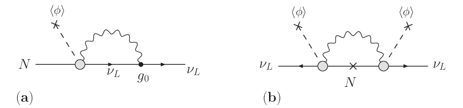
Refer to caption
Figure 4.9: Contribution to (a) the neutrino Dirac mass and (b) the neutrino Majorana mass induced by the dim-6 transition EMDM operator. Here g0g_{0} and ⟨ϕ⟩\langle\phi\rangle denote the gauge coupling constant and Higgs VEV respectively.

Unfortunately, the exact size of these contributions cannot be calculated in a model-independent way because one would require the precise relationship between the dipole moments and mass terms, which can only be resolved if the nature of the new physics at scale Λ\Lambda is specified. However, an estimate of these quantities can be obtained by applying simple dimensional analysis. To this end, we begin by writing down the approximate form of the amplitude for the Dirac mass diagram in Fig. 4.9a, ignoring the external lines (i.e. setting their momentum to zero) and factors of ±i\pm i:

mD\displaystyle m_{D} ∼∫Λd4​k(2​π)4​(g0​γμ)​gμ​νk2+i​ϵ​k̸+mk2−m2+i​ϵ​(2​λ0′​⟨ϕ⟩Λ2​PR​σα​ν​kα),\displaystyle\sim\int^{\Lambda}\frac{d^{4}k}{(2\pi)^{4}}\left(g_{0}\gamma^{\mu}\right)\frac{g_{\mu\nu}}{k^{2}+i\epsilon}\,\frac{\not{k}+m}{k^{2}-m^{2}+i\epsilon}\left(\frac{2\,\lambda_{0}^{\prime}\,\langle\phi\rangle}{\Lambda^{2}}\,P_{R}\,\sigma^{\alpha\nu}\,k_{\alpha}\right)\;,
≃λ0′​g0​⟨ϕ⟩(2​π)4​Λ2​∫Λd4​k​1k2​1k2−m2​γμ​(k̸+m)​PR​(k̸​γμ−γμ​k̸)⏟≃PR​(k2+m​k̸),\displaystyle\simeq\frac{\lambda_{0}^{\prime}\,g_{0}\,\langle\phi\rangle}{(2\pi)^{4}\Lambda^{2}}\int^{\Lambda}d^{4}k\;\frac{1}{k^{2}}\,\frac{1}{k^{2}-m^{2}}\underbrace{\gamma^{\mu}(\not{k}+m)\,P_{R}\,(\not{k}\gamma_{\mu}-\gamma_{\mu}\not{k})}_{\simeq P_{R}(k^{2}+m\not{k})}\;, (4.111)

where kk is the loop momentum and mm is the mass of νL\nu_{L}. In the limit of m→0m\rightarrow 0 and after dropping the projection operator, PRP_{R} from the expression, we then have

mD\displaystyle m_{D} ∼λ0′​g0​⟨ϕ⟩(2​π)4​Λ2​∫Λd4​k​1k2,\displaystyle\sim\frac{\lambda_{0}^{\prime}\,g_{0}\,\langle\phi\rangle}{(2\pi)^{4}\Lambda^{2}}\int^{\Lambda}d^{4}k\;\frac{1}{k^{2}}\;,
≃λ0′​g0​⟨ϕ⟩(2​π)4​Λ2​∫Λ(dk)2​k2​dΩ​1k2⏟≃π2​Λ2,\displaystyle\simeq\frac{\lambda_{0}^{\prime}\,g_{0}\,\langle\phi\rangle}{(2\pi)^{4}\Lambda^{2}}\underbrace{\int^{\Lambda}(dk)^{2}k^{2}d\Omega\,\frac{1}{k^{2}}}_{\simeq\,\pi^{2}\Lambda^{2}}\;,
≃λ0′​g0​⟨ϕ⟩16​π2.\displaystyle\simeq\frac{\lambda_{0}^{\prime}\,g_{0}\,\langle\phi\rangle}{16\pi^{2}}\;. (4.112)

This Dirac mass term together with the heavy neutrino Majorana mass (MM) can give rise to a light neutrino Majorana mass via the type I seesaw mechanism (see Sec. 1.2.3) with the form

mν(1)=mD​M−1​mDT≃(g0​⟨ϕ⟩16​π2)2​λ0′​M−1​(λ0′)T.m^{(1)}_{\nu}=m_{D}\,M^{-1}\,m_{D}^{T}\,\simeq\,\left(\frac{g_{0}\,\langle\phi\rangle}{16\pi^{2}}\right)^{2}\lambda_{0}^{\prime}\,M^{-1}\,(\lambda^{\prime}_{0})^{T}\;. (4.113)

Similarly, we can deduce the direct contribution to the light neutrino Majorana mass term coming from the loop diagram in Fig. 4.9b via the following estimate of its amplitude:

mν(2)\displaystyle m_{\nu}^{(2)} ∼∫Λd4​k(2​π)4​(2​λ0′​⟨ϕ⟩Λ2​PR​σα​ν​kα)​gμ​νk2+i​ϵ​k̸+Mk2−M2+i​ϵ​(kβ​σβ​μ​PR​2​(λ0′)T​⟨ϕ⟩Λ2),\displaystyle\sim\int^{\Lambda}\frac{d^{4}k}{(2\pi)^{4}}\left(\frac{2\,\lambda_{0}^{\prime}\,\langle\phi\rangle}{\Lambda^{2}}\,P_{R}\,\sigma^{\alpha\nu}k_{\alpha}\right)\frac{g_{\mu\nu}}{k^{2}+i\epsilon}\,\frac{\not{k}+M}{k^{2}-M^{2}+i\epsilon}\left(k_{\beta}\sigma^{\beta\mu}\,P_{R}\,\frac{2\,(\lambda_{0}^{\prime})^{T}\,\langle\phi\rangle}{\Lambda^{2}}\right)\;, (4.114)

where we have omitted all the charge conjugation operators, CC in the definition of the Majorana propagator and from transposing for convenience. Note that this omission is inconsequential to our final outcome as the operator CC can always be absorbed into the external fields via relations such as u=C​v¯Tu=C\overline{v}^{T} and v=C​u¯Tv=C\overline{u}^{T} for any generic spinors. Simplifying (4.114) using standard contraction identities for gamma matrices, we get

mν(2)\displaystyle m_{\nu}^{(2)} ∼λ0′​⟨ϕ⟩2(2​π)4​Λ4​∫Λd4​kk2​(k2−M2)​PR​(k̸​γμ−γμ​k̸)​(k̸+M)​(k̸​γμ−γμ​k̸)​PR⏟≃PR​M​k2​(λ0′)T,\displaystyle\sim\frac{\lambda_{0}^{\prime}\,\langle\phi\rangle^{2}}{(2\pi)^{4}\Lambda^{4}}\int^{\Lambda}\frac{d^{4}k}{k^{2}\,(k^{2}-M^{2})}\,\underbrace{P_{R}\,(\not{k}\gamma_{\mu}-\gamma_{\mu}\not{k})\,(\not{k}+M)\,(\not{k}\gamma^{\mu}-\gamma^{\mu}\not{k})\,P_{R}}_{\simeq\,P_{R}Mk^{2}}\;(\lambda_{0}^{\prime})^{T}\;,
≃λ0′​⟨ϕ⟩2(2​π)4​Λ4​∫Λ(dk)2​k2​dΩ​Mk2−M2⏟≃π2​M​Λ2​(λ0′)T,\displaystyle\simeq\frac{\lambda_{0}^{\prime}\,\langle\phi\rangle^{2}}{(2\pi)^{4}\Lambda^{4}}\underbrace{\int^{\Lambda}(dk)^{2}k^{2}d\Omega\;\frac{M}{k^{2}-M^{2}}}_{\simeq\,\pi^{2}M\Lambda^{2}}\;(\lambda_{0}^{\prime})^{T}\;,
≃⟨ϕ⟩216​π2​Λ2​λ0′​M​(λ0′)T.\displaystyle\simeq\frac{\langle\phi\rangle^{2}}{16\pi^{2}\Lambda^{2}}\;\lambda_{0}^{\prime}\,M\,(\lambda_{0}^{\prime})^{T}\;. (4.115)

Generically, one can expect that both (4.113) and (4.115) will add to the effective light neutrino Majorana mass although the contribution arising from (4.115) is typically dominant (unless Λ≫M\Lambda\gg M) due to the extra 1/16​π21/16\pi^{2} suppression factor in the definition of (4.113). But in any case, this connection between the EMDM couplings, λ0′\lambda_{0}^{\prime}, and neutrino masses presents an important constraint that can control the size of the C​PCP asymmetry arising from electromagnetic leptogenesis, as we shall discuss in the following.

4.4.2 Discussion on the parameter space

As a result of the link between the EMDM couplings and light neutrino masses, we may derive a lower limit on the size of M1M_{1}, just like (1.131) on page 1.131 for standard N1N_{1}-leptogenesis. This is because there exists a relationship between |ε1EM|max|\varepsilon_{1}^{\text{EM}}|_{\text{max}} and M1M_{1}, which is analogous to that of (1.104) on page 1.104, with the role of the Yukawa coupling matrix, hh being replaced by λ0′\lambda_{0}^{\prime}. Using Eqs. (4.110) and (4.115) with the assumptions |(λ0′)j​k|≤|(λ0′)33||(\lambda_{0}^{\prime})_{jk}|\leq~\!|(\lambda_{0}^{\prime})_{33}| and M1≪M2,3M_{1}\ll M_{2,3}, we can retrace the steps leading to (1.104) and obtain

|ε1EM|max∼10−6​βΛ4​(M11010​GeV),|\varepsilon_{1}^{\text{EM}}|_{\text{max}}\sim 10^{-6}\,\beta_{\Lambda}^{4}\left(\frac{M_{1}}{10^{10}~\text{GeV}}\right)\;, (4.116)

where we have taken M≡M3≃ΛM\equiv M_{3}\simeq\Lambda in (4.115), and defined the quantity, βΛ≡M1/Λ\beta_{\Lambda}\equiv M_{1}/\Lambda which indicates the level of hierarchy among the RH neutrinos. From (4.116), a couple of general observations for electromagnetic leptogenesis can be made. Firstly, it is clear that to obtain a reasonable size for the C​PCP asymmetry (e.g. 𝒪⁡(10−6)\mathcal{O}\left(10^{-6}\right)), the scale for M1M_{1} must be at least 𝒪⁡(1010)\mathcal{O}\left(10^{10}\right) GeV, a result which is similar to that from standard N1N_{1}-leptogenesis 2020 20 It should be noted that although the scenario of TeV scale leptogenesis discussed in Ref. [179] involves 3-body decay processes, these are inherently different from the interactions we have investigated in the EMDM model. In the case of Ref. [179], the 3-body decays studied are one-loop processes whereas ours involves two-loop graphs.. Secondly, the presence of the suppression factor, βΛ4\beta_{\Lambda}^{4} implies that a strong RH neutrino mass hierarchy is in general undesirable as M1≪M3≃ΛM_{1}\ll M_{3}\simeq\Lambda automatically means βΛ4≪1\beta_{\Lambda}^{4}\ll 1. Hence, in order to acquire a sufficiently large raw C​PCP asymmetry together with experimentally acceptable light neutrino masses, some very mild fine-tunning between the scales of MiM_{i} and Λ\Lambda, as well as the absolute size of the coupling λ0′\lambda_{0}^{\prime} is required. Qualitatively speaking though, the conditions governing electromagnetic leptogenesis (modulo the suppression factor) are largely identical to the standard Yukawa-mediated case. To summarize the situation, we compare the various key quantities resulting from the EMDM model with the corresponding ones for the standard scenario in Table 4.1.

Standard Electromagnetic
Γ1=116​π​(h†​h)11​M1\Gamma_{1}=\dfrac{1}{16\pi}\,(h^{\dagger}h)_{11}M_{1} Γ1EM=14​π​(λ0′⁣†​λ0′)11​M1​(M128​π​Λ2)2\Gamma_{1}^{\text{EM}}=\dfrac{1}{4\pi}\,(\lambda_{0}^{\prime\dagger}\lambda_{0}^{\prime})_{11}M_{1}\left(\dfrac{M_{1}^{2}}{8\pi\Lambda^{2}}\right)^{2}
|ε1|≃1π​∑m≠1Im(h†h)21​m](h†​h)11​M1Mm\displaystyle{|\varepsilon_{1}|\simeq\frac{1}{\pi}\,\sum_{m\neq 1}\frac{\textrm{Im}\,(h^{\dagger}h)^{2}_{1m}]}{(h^{\dagger}h)_{11}}\frac{M_{1}}{M_{m}}} |ε1EM|≃1π​∑m≠1Im​[(λ0′⁣†​λ0′)1​m2](λ0′⁣†​λ0′)11​M1Mm​(M128​π​Λ2)2\displaystyle{|\varepsilon_{1}^{\text{EM}}|\simeq\frac{1}{\pi}\,\sum_{m\neq 1}\frac{\textrm{Im}\,[(\lambda_{0}^{\prime\dagger}\lambda_{0}^{\prime})^{2}_{1m}]}{(\lambda_{0}^{\prime\dagger}\lambda_{0}^{\prime})_{11}}\frac{M_{1}}{M_{m}}}\left(\frac{M_{1}^{2}}{8\pi\Lambda^{2}}\right)^{2}
mν∼⟨ϕ⟩2​h​M−1​hT\displaystyle{m_{\nu}\sim\langle\phi\rangle^{2}\,h\,M^{-1}\,h^{T}} mνEM∼⟨ϕ⟩216​π2​[g0216​π2​λ0′​M−1​(λ0′)T+1Λ2​λ0′​M​(λ0′)T]\displaystyle{m_{\nu}^{\text{EM}}\sim\frac{\langle\phi\rangle^{2}}{16\pi^{2}}\left[\frac{g_{0}^{2}}{16\pi^{2}}\,\lambda_{0}^{\prime}\,M^{-1}\,(\lambda_{0}^{\prime})^{T}+\frac{1}{\Lambda^{2}}\,\lambda_{0}^{\prime}\,M\,(\lambda_{0}^{\prime})^{T}\right]}
Table 4.1: Comparison of key quantities in standard and electromagnetic leptogenesis, where hh and λ0′\lambda_{0}^{\prime} denote the Yukawa and dimensionless EMDM coupling constants. We have assumed there is at least a mild hierarchy in the masses of the heavy neutrinos, such that the asymmetry is predominantly generated from the decay of the lightest state, N1N_{1}.

In a model where both the Yukawa and EMDM interactions are present in the Lagrangian, we have, in general, contributions to the decay rate, C​PCP asymmetry and neutrino mass coming from both the standard and electromagnetic sectors. As a result, either one mechanism will dominate, or there will be an interplay between the two, depending on the relative size of hh and λ0′\lambda_{0}^{\prime} (and perhaps other factors). For our investigation here, we are particularly interested in examining if electromagnetic leptogenesis alone (i.e. when the Yukawa couplings are negligible) can give rise to the required asymmetry without contradicting any known experimental constraints. To this end, we select some representative input parameters for the EMDM model and study their implications.

Given that electromagnetic leptogenesis does not seem to favor a very strong hierarchy in the RH neutrino mass spectrum, as well as between MM and Λ\Lambda, we shall adopt the values

Λ≃10​M2,3≃20​M1,\Lambda\simeq 10M_{2,3}\simeq 20M_{1}\;, (4.117)

as an illustrative example. In addition, we shall (for simplicity) make the crude assumption that all elements of the matrix λ0′\lambda_{0}^{\prime} are of similar magnitude, and ignoring any flavor structures it (as well as mνm_{\nu} and MM) may possess. With these, it is straight forward to check using the expression for |ε1EM||\varepsilon_{1}^{\text{EM}}| in Table 4.1 that a value of

λ0′≃35,\lambda_{0}^{\prime}\simeq 35\;, (4.118)

for the EMDM coupling is sufficient to the produce an asymmetry of |ε1EM|∼10−6|\varepsilon_{1}^{\text{EM}}|\sim 10^{-6}. To understand the general behavior of washout, we can follow the standard leptogenesis analysis and define the decay parameter (see (2.49) on page 2.49):

K1=Γ1EMH⁡(T=M1),K_{1}=\frac{\Gamma_{1}^{\text{EM}}}{H(T=M_{1})}\;, (4.119)

where HH is the Hubble parameter as defined in (2.47) on page 2.47. Recall that K1K_{1} controls whether the N1N_{1} decays are in equilibrium, and is also a measure of washout effects via inverse decay. For definiteness, if we set

M1≃5×10¹²​GeV,M_{1}\simeq 5\times 10^{12}~\text{GeV}\;, (4.120)

then the parameters in (4.117) and (4.118) imply that K1≃0.3K_{1}\simeq 0.3. As we know from Chapter 2, K1≪1K_{1}\ll 1 (K1≫1K_{1}\gg 1) corresponds to the weak (strong) washout regime, hence this parameter choice for the EMDM model should lead to a moderate washout of the asymmetry 2121 21 A detailed study of washout effects is beyond the scope of this work.. So, qualitatively speaking, we expect that successful electromagnetic leptogenesis is achievable with these parameter choices.

The implications for the light neutrino mass can be readily obtained using the two terms for mνEMm_{\nu}^{\text{EM}} in Table 4.1, and one finds

mν(1)≃4×10⁻²​eV,mν(2)≃1×10⁻¹​eV,m_{\nu}^{(1)}\simeq 4\times 10^{-2}~\text{eV}\;,\qquad m_{\nu}^{(2)}\simeq 1\times 10^{-1}~\text{eV}\;, (4.121)

where we have set g0≡g′g_{0}\equiv g^{\prime}. In evaluating the numerical values for g′g^{\prime}, we have used MW=g⁡⟨ϕ⟩/2≃80M_{W}=g\langle\phi\rangle/\sqrt{2}\simeq 80 GeV and MZ=⟨ϕ⟩​(g2+g′2)/2≃91M_{Z}=\langle\phi\rangle\sqrt{(g^{2}+g^{\prime 2})/2}\simeq 91 GeV with ⟨ϕ⟩=174\langle\phi\rangle=174 GeV. It is worth pointing out that, as expected, the direct contribution to the Majorana mass term, mν(2)m_{\nu}^{(2)} (Fig. 4.9b) dominates over mν(1)m_{\nu}^{(1)} (Fig. 4.9a).

Finally, we note that the presence of the EMDM operators in the model will not only give rise to transition moments between a light and a heavy neutrino, they will also induce effective dipole moment interactions between two light neutrino states via two-loop diagrams such as the one depicted in Fig. 4.10. Therefore, it is imperative to check that this contribution to the light neutrino dipole moments is not in conflict with the current experimental upper limits, when we take the particular input values assumed above.

Applying dimensional analysis and assuming the worst case scenario where all quantities in the numerator with unit of mass are replaced by the cut-off scale Λ\Lambda, we estimate the amplitude of Fig. 4.10 as

μνeff\displaystyle\mu_{\nu}^{\text{eff}} ∼g0(16​π2)2​λ0′Λ2​λ0′Λ2×Λ3,\displaystyle\sim\frac{g_{0}}{(16\pi^{2})^{2}}\,\frac{\lambda_{0}^{\prime}}{\Lambda^{2}}\,\frac{\lambda_{0}^{\prime}}{\Lambda^{2}}\times\Lambda^{3}\;,
=g0​(λ0′16​π2)2​1Λ.\displaystyle=g_{0}\left(\frac{\lambda_{0}^{\prime}}{16\pi^{2}}\right)^{2}\,\frac{1}{\Lambda}\;. (4.122)

Substituting in the value for Λ\Lambda assumed previously, and expressing in units of the Bohr magneton, μB=e/2​me≃3×10−7​ eV−1\mu_{B}=e/2m_{e}\simeq 3\times 10^{-7}\text{ eV}^{-1}, we have μνeff∼5×10⁻¹⁹​μB\mu_{\nu}^{\text{eff}}\sim 5\times 10^{-19}\,\mu_{B}. So, it is well within the current experimental limits which are of 𝒪⁡(10−11​μB)\mathcal{O}\left(10^{-11}\,\mu_{B}\right) [11, 60, 61].

Refer to caption
Figure 4.10: An example of a two-loop digram that contributes to the effective light neutrino dipole moments.

It is worth mentioning that when the Yukawa couplings are switched on, there will be additional contributions to these effective light neutrino dipole moments originating from light and heavy neutrino mixings. However, such contributions are hugely suppressed by a factor of ⟨ϕ⟩2​Λ−2​M−1\langle\phi\rangle^{2}\Lambda^{-2}M^{-1} (instead of Λ−1\Lambda^{-1} as in (4.122)), and so their effects will be sub-dominant.

In summary, we have demonstrated that there is a region of parameter space where electromagnetic leptogenesis is viable, thus providing a new alternative that can stand alone or complement the standard scenario.

4.5  Summary and outlook

The inclusion of the heavy RH neutrinos to the SM has not only provided an elegant way to generate small neutrino masses via the type I seesaw mechanism, it has also opened up many new possibilities for model builders. In this chapter, we have seized upon this and investigated the natural extension of introducing electromagnetic dipole moment interactions between the heavy RH neutrinos and their light counterparts. One immediate result is that lepton violating decays of the heavy neutrinos are no longer solely mediated by the Yukawa term, but also by the newly included EMDM operators. Consequently, it is of great interest to ascertain whether such radiative decay is capable of creating a cosmic baryon asymmetry in a similar way to that of standard leptogenesis.

By carefully studying the properties of the EMDM couplings and explicitly calculating the decay amplitudes for the tree-level and interference terms, we have shown that, in general, the C​PCP asymmetry induced by the EMDM operators is nonzero. As a result, we have proved that, in principle at least, electromagnetic leptogenesis can be a viable mechanism for generating a lepton asymmetry in the early universe.

Furthermore, in order to embed this model into the SM, a realistic generalisation to the basic dimension-5 EMDM operator has also been investigated. The end result is that this new scenario of leptogenesis is very much akin to the standard case, except that the role of the Yukawa couplings is now played by their EMDM counterparts, and there is an additional suppression factor (∼M2/Λ2\sim M^{2}/\Lambda^{2}) since the EMDM operator is of higher dimension. Because of the presence of this suppression, the region of applicability for leptogenesis is slightly different in the EMDM scenario, and it disfavors a strong hierarchy in the RH neutrino mass spectrum. Moreover, washout effects in this model will differ from the standard case since the principle LL violating processes all have a 3-body initial or final state and involve a vector boson, hence the set of interactions participating in washout will be drastically different.

Other constraints on the model come from the light neutrino mass and effective dipole moment terms induced by loop diagrams involving the EMDM operators. These contributions directly restrict the magnitude of the EMDM coupling allowed, although the latter effects are normally not as significant due to the heaviness of Λ\Lambda. In fact, we have discovered that the constraints from the neutrino mass terms demand that the scale of MM, hence Λ\Lambda, must be at least of 𝒪⁡(1010)\mathcal{O}\left(10^{10}\right) GeV to produce a mνm_{\nu} at the correct scale while maintaining a reasonably sized |εEM||\varepsilon^{\text{EM}}|. Thus, the conditions imposed by the effective light neutrino dipole contribution are usually unimportant for most viable input parameters.

In addition, this result implies a typical leptogenesis temperature of T∼1010T\sim 10^{10} GeV, which is comparable to the usual case. Consequently, it opens up an intriguing (but yet to be explored) possibility of Yukawa-EMDM interplay in the generation of lepton number. Indeed, there is a plethora of new ideas and issues one may further study on this topic. For instance, in the specific analysis, the flavor structure of the EMDM couplings, λ0′\lambda_{0}^{\prime} has not been included. Therefore, an investigation of λ0′\lambda_{0}^{\prime} similar to that for the Yukawas, hh (or the seesaw orthogonal matrix, Ω\Omega discussed in Sec. 1.4.3 and in Chapter 2) would be worthwhile. Also, owing to the fact that a strongly hierarchical RH neutrino spectrum is undesirable for electromagnetic leptogenesis, it would be quite natural to study the scenario where the RH neutrinos are quasi-degenerate, where resonant effects (see Sec. 1.4.4) in the radiative decays may become important. Finally, there is a possibility that the newly included EMDM operators can give rise to non-trivial interactions between all neutrino species and the primordial magnetic field in the thermal plasma, hence affecting the evolution of lepton number.

But even without venturing into these complications, our work here has demonstrated that a new scenario beyond the standard leptogenesis framework (due to transition neutrino dipole moments) is viable, and it provides yet another example of the important link between neutrino properties and cosmology.

Chapter 5 Conclusion

On e of the most fundamental concepts in the study of physics is the idea of symmetry. Yet, Nature as we know it does not always seem to be perfectly symmetrical. Indeed, the principal theme for this current work is motivated by none other than the apparent asymmetry between matter and antimatter in the universe. Therefore, along with the appeal of symmetry, a major topic of interest is the mechanism of symmetry breaking or asymmetry creation.

For the cosmic baryon asymmetry, this presents a unique challenge as the study of baryogenesis inevitably brings together the two giants of particle physics and Big Bang cosmology. To date though the solution to this puzzle is still highly speculative, and in the absence of more experimental inputs, it may remain unresolved for some time to come. Owing to this, the choice of the model employed is often based entirely on its theoretical appeal, as well as the prejudices of the investigator. It is fair to say that our approach of taking leptogenesis as the correct answer to the baryogenesis problem throughout this work is no exception, and it is strongly influenced by our interest in neutrino physics.

Without a doubt, it is quite fascinating that two seemingly unrelated problems— the tiny masses of light neutrino and the matter-antimatter asymmetry— may be explained in a consistent manner by the mere introduction of heavy RH neutrinos to the SM. As we have seen in our earlier discussions, the former may be explained by the type I seesaw mechanism while thermal leptogenesis provides an attractive solution to the later. This naturally means that an intricate link between neutrino properties and the baryon asymmetry can be established. Consequently, it has been the purpose of this work to explore the implications of several different neutrino models in the leptogenesis context.

Taking the type I seesaw framework (with three heavy RH neutrinos) as the starting point, we investigated three distinct possibilities in extending the typical setup for the neutrino sector, and studied their connection to the generation of lepton asymmetry. In the first part of our work, we performed a comprehensive analysis on the leptogenesis implications of the neutrino models proposed in Ref. [129]. These models have the advantage of requiring less free parameters to define the theory than the default seesaw setup, a unique feature which is made possible by the imposition of an abelian family symmetry and the inclusion of a new Higgs singlet. As a corollary, θ13=0\theta_{13}=0 in the UPMNSU_{\text{PMNS}} matrix, as well as a fully hierarchical light neutrino spectrum are predicted. Since it is the leptogenesis credentials of these models that interest us, we have carefully identified all the key ingredients which can modify the overall scenario for lepton production, and compared how each element may differ in its predictions from those in the standard seesaw. The general conclusion we obtained is that having an extra abelian symmetry and singlet Higgs do not hinder the possibility of successful leptogenesis in these setups. In fact, their predictions are largely identical to the default case for both unflavored and flavored N1N_{1}-leptogenesis. Consequently, this shows another important feature of these economical seesaw models.

In the second part of our work, we noted that conventional type I seesaw inevitably gives rise to a largely unconstrained heavy RH seesaw sector, hence making it difficult to experimentally test this mass generation mechanism. Moreover, given the close relationship between neutrino models and leptogenesis, one would like to ascertain more information from the seesaw sector. Therefore, it is well-motivated to explore the possibility of constraining the heavy seesaw sector so that it is completely determined by low-energy observables. The strategy we employed in tackling this involves combining the powers of an expanded gauge group and an inter-generational flavor symmetry such that the former can enforce the desired mass relations while the latter leads to predictable diagonalization matrices. Subsequently, the simplest models of this type lead to a RH neutrino mass matrix that can be written in terms of only low-energy fermion masses, mixing angles and C​PCP phases:

MR≃m^fUPMNS∗m^ν−1UPMNS†m^f,where f=e,d,u.M_{R}\simeq\widehat{m}_{f}\,U_{\text{PMNS}}^{*}\,\widehat{m}_{\nu}^{-1}\,U_{\text{PMNS}}^{\dagger}\,\widehat{m}_{f}\;,\qquad\text{where }f=e,d,u\;.

In the representative models that we have constructed to achieve the above relation, it has been found that successful leptogenesis is only possible in a very fine-tuned region of the parameter space. Specifically, one must select the f=uf=u case, as well as certain combinations of Dirac and Majorana phases in UPMNSU_{\text{PMNS}} such that a lepton asymmetry can be generated via either resonant or flavored N2N_{2}-leptogenesis. Furthermore, it has been shown that although the f=ef=e case can yield a TeV scale RH neutrino, the probability of detecting it at the LHC or a next-generation collider such as the ILC is far too small.

But it is enlightening to note that this part of our work has demonstrated the ability of symmetries to bridge the missing link between the heavy seesaw sector and experimentally accessible parameters. In addition, it is highly probable that, with a different choice of the underlying symmetry and Higgs structure as shown here, interesting phenomenology can result and potentially provide new hints on building realistic neutrino seesaw models that are experimentally verifiable.

Finally, in the last part of our work, we investigated the effects of introducing an effective transition electromagnetic dipole moment operator between the LH light and RH heavy neutrinos. Since nonzero neutrino dipole moments are a direct consequence of having massive neutrinos, the inclusion of RH neutrinos to the SM via type I seesaw immediately opens up the possibility of active-sterile neutrino transition moments. Such interactions are potentially important in cosmology because the radiative decay of the heavy RH neutrino (N→ν​γN\rightarrow\nu\,\gamma) violates lepton number, and in general, C​PCP . As a result, a new scenario for leptogenesis whereby the lepton asymmetry is solely generated by the EMDM-type (instead of the usual Yukawa-mediated) interactions is possible. By exploring the key ingredients leading to C​PCP violation, we have shown by explicit computations of the relevant diagrams in a toy model that, in principle, electromagnetic leptogenesis is a viable alternative for creating a lepton asymmetry.

Eventually, to build a realistic theory that can be embedded into the SM, the simplistic setup was generalized such that it became compatible with the SM gauge group. Although in this case all relevant processes involved consisted of 3-body initial or final states, it has been found that a nonzero C​PCP asymmetry can still be generated, and that the effect of the suppression factor due to 3-body phase space can be reduced by the appropriate choice of the RH neutrino mass hierarchy. In fact, this scenario disfavors the usual strongly hierarchical RH mass spectrum normally assumed for standard leptogenesis. However, we have demonstrated that for a mild hierarchy, where N1N_{1}-leptogenesis is still a good approximation, there exists a workable parameter space where electromagnetic leptogenesis alone can produce the necessary lepton asymmetry to solve the baryogenesis problem. In addition, foregoing the hierarchical requirement completely and having quasi-degenerate RH neutrinos is perfectly acceptable, and perhaps even more desirable in some situations as resonant effects can open up a larger region for successful electromagnetic leptogenesis. So, there is no doubt that transition EMDM interactions between light and heavy neutrinos can have far-reaching consequences in the early universe.

In conclusion, this work has further highlighted the already well-known fact of the inseparability between neutrino physics and cosmology. Even though we have only explored a tiny region of these two vast topics, it is nonetheless enlightening to witness the richness of ideas allowed and motivated by them through our meticulous investigations. It is true however that many important questions remain to be answered, and therefore we await the new data which will come with future technological advances to inform us of the model that really represents how Nature works.

List of Publications

  1. 1.

    S. S. C. Law and R. R. Volkas,
    Leptogenesis implications in models with Abelian family symmetry and one extra real Higgs singlet,
    Phys. Rev. D 75, 043510 (2007) [arXiv:hep-ph/0701189].

  2. 2.

    N. F. Bell, B. J. Kayser and S. S. C. Law,
    Electromagnetic Leptogenesis,
    Phys. Rev. D 78, 085024 (2008) [arXiv:0806.3307 [hep-ph]]

  3. 3.

    X. G. He, S. S. C. Law and R. R. Volkas,
    Determining the heavy seesaw neutrino mass matrix from low-energy parameters,
    Phys. Rev. D 78, 113001 (2008) [arXiv:0810.1104 [hep-ph]].

Bibliography

  • [1] R. J. Davis, D. S. Harmer and K. C. Hoffman, Phys. Rev. Lett. 20, 1205 (1968); and later with the improved facility at the same site: B. T. Cleveland et al., Astrophys. J. 496, 505 (1998).
  • [2] J. N. Bahcall, W. A. Fowler, I. Iben and R. L. Sears, Astrophys. J. 137, 344 (1963); see also J. N. Bahcall, M. H. Pinsonneault and S. Basu, Astrophys. J. 555, 990 (2001) [arXiv:astro-ph/0010346].
  • [3] K. S. Hirata et al. [KAMIOKANDE-II Collaboration], Phys. Rev. Lett. 63, 16 (1989); K. S. Hirata et al. [KAMIOKANDE-II Collaboration], Phys. Rev. Lett. 65, 1297 (1990); K. S. Hirata et al. [KAMIOKANDE-II Collaboration], Phys. Rev. Lett. 65, 1301 (1990).
  • [4] Y. Fukuda et al. [Kamiokande Collaboration], Phys. Rev. Lett. 77, 1683 (1996).
  • [5] S. Fukuda et al. [Super-Kamiokande Collaboration], Phys. Rev. Lett. 86, 5651 (2001) [arXiv:hep-ex/0103032]; S. Fukuda et al. [Super-Kamiokande Collaboration], Phys. Rev. Lett. 86, 5656 (2001) [arXiv:hep-ex/0103033].
  • [6] P. Anselmann et al. [GALLEX Collaboration], Phys. Lett. B 285, 376 (1992); W. Hampel et al. [GALLEX Collaboration], Phys. Lett. B 447, 127 (1999); M. Altmann et al. [GNO Collaboration], Phys. Lett. B 490, 16 (2000) [arXiv:hep-ex/0006034]; M. Altmann et al. [GNO COLLABORATION Collaboration], Phys. Lett. B 616, 174 (2005) [arXiv:hep-ex/0504037].
  • [7] D. N. Abdurashitov et al., Phys. Lett. B 328, 234 (1994); J. N. Abdurashitov et al. [SAGE Collaboration], Phys. Rev. C 60, 055801 (1999) [arXiv:astro-ph/9907113]; J. N. Abdurashitov et al. [SAGE Collaboration], Phys. Rev. Lett. 83, 4686 (1999) [arXiv:astro-ph/9907131]; J. N. Abdurashitov et al. [SAGE Collaboration], J. Exp. Theor. Phys. 95, 181 (2002) [Zh. Eksp. Teor. Fiz. 122, 211 (2002)] [arXiv:astro-ph/0204245].
  • [8] L. Wolfenstein, Phys. Rev. D 17, 2369 (1978); S. P. Mikheyev, A. Yu. Smirnov, Yad. Fiz. 42, 1441 (1985) [Sov. J. Nucl. Phys. 42, 913 (1985)]; S. P. Mikheyev, A. Yu. Smirnov, Nuovo Cimento 9C, 17 (1986).
  • [9] Q. R. Ahmad et al. [SNO Collaboration], Phys. Rev. Lett. 87, 071301 (2001) [arXiv:nucl-ex/0106015]; Q. R. Ahmad et al. [SNO Collaboration], Phys. Rev. Lett. 89, 011301 (2002) [arXiv:nucl-ex/0204008]; Q. R. Ahmad et al. [SNO Collaboration], Phys. Rev. Lett. 89, 011302 (2002) [arXiv:nucl-ex/0204009].
  • [10] K. Eguchi et al. [KamLAND Collaboration], Phys. Rev. Lett. 90, 021802 (2003) [arXiv:hep-ex/0212021]; T. Araki et al. [KamLAND Collaboration], Phys. Rev. Lett. 94, 081801 (2005) [arXiv:hep-ex/0406035]; S. Abe et al. [KamLAND Collaboration], Phys. Rev. Lett. 100, 221803 (2008) [arXiv:0801.4589 [hep-ex]].
  • [11] C. Arpesella et al. [Borexino Collaboration], Phys. Lett. B 658, 101 (2008) [arXiv:0708.2251 [astro-ph]]; Phys. Rev. Lett. 101, 091302 (2008) [arXiv:0805.3843 [astro-ph]].
  • [12] T. J. Haines et al., Phys. Rev. Lett. 57, 1986 (1986); D. Casper et al., Phys. Rev. Lett. 66, 2561 (1991); R. Becker-Szendy et al., Phys. Rev. D 46, 3720 (1992).
  • [13] K. S. Hirata et al. [KAMIOKANDE-II Collaboration], Phys. Lett. B 205, 416 (1988); Y. Fukuda et al. [Kamiokande Collaboration], Phys. Lett. B 335, 237 (1994).
  • [14] Y. Fukuda et al. [Super-Kamiokande Collaboration], Phys. Rev. Lett. 81, 1562 (1998) [arXiv:hep-ex/9807003]; Y. Fukuda et al. [Super-Kamiokande Collaboration], Phys. Lett. B 436, 33 (1998) [arXiv:hep-ex/9805006]; Y. Fukuda et al. [Super-Kamiokande Collaboration], Phys. Rev. Lett. 82, 2644 (1999) [arXiv:hep-ex/9812014].
  • [15] M. H. Ahn et al. [K2K Collaboration], Phys. Rev. D 74, 072003 (2006) [arXiv:hep-ex/0606032].
  • [16] D. G. Michael et al. [MINOS Collaboration], Phys. Rev. Lett. 97, 191801 (2006) [arXiv:hep-ex/0607088]; P. Adamson et al. [MINOS Collaboration], arXiv:0806.2237 [hep-ex].
  • [17] B. Pontecorvo, Sov. Phys. JETP 6, 429 (1957) [Zh. Eksp. Teor. Fiz. 33, 549 (1957)]; B. Pontecorvo, Sov. Phys. JETP 7, 172 (1958) [Zh. Eksp. Teor. Fiz. 34, 247 (1957)]; Z. Maki, M. Nakagawa and S. Sakata, Prog. Theor. Phys. 28, 870 (1962).
  • [18] See for example: H. J. Lipkin, Phys. Lett. B 579, 355 (2004) [arXiv:hep-ph/0304187]; L. Stodolsky, Phys. Rev. D 58, 036006 (1998) [arXiv:hep-ph/9802387].
  • [19] C. Athanassopoulos et al. [LSND Collaboration], Phys. Rev. Lett. 77, 3082 (1996) [arXiv:nucl-ex/9605003]; C. Athanassopoulos et al. [LSND Collaboration], Phys. Rev. Lett. 81, 1774 (1998) [arXiv:nucl-ex/9709006].
  • [20] A. Bazarko [MiniBooNE Collaboration], Nucl. Phys. Proc. Suppl. 91, 210 (2001) [arXiv:hep-ex/0009056]; A. O. Bazarko [BooNe Collaboration], arXiv:hep-ex/9906003; arXiv:hep-ex/0210020; M. H. Shaevitz [MiniBooNE Collaboration], Nucl. Phys. Proc. Suppl. 137, 46 (2004) [arXiv:hep-ex/0407027]; Z. Djurcic [MiniBooNE Collaboration], Nucl. Phys. Proc. Suppl. 168, 309 (2007) [arXiv:hep-ex/0701017]; M. Maltoni and T. Schwetz, Phys. Rev. D 76, 093005 (2007) [arXiv:0705.0107 [hep-ph]].
  • [21] M. Apollonio et al. [CHOOZ Collaboration], Eur. Phys. J. C 27, 331 (2003) [arXiv:hep-ex/0301017]; M. Apollonio et al. [CHOOZ Collaboration], Phys. Lett. B 466, 415 (1999) [arXiv:hep-ex/9907037]; M. Apollonio et al. [CHOOZ Collaboration], Phys. Lett. B 420, 397 (1998) [arXiv:hep-ex/9711002].
  • [22] M. Kobayashi and T. Maskawa, Prog. Theor. Phys. 49, 652 (1973); N. Cabibbo, Phys. Rev. Lett. 10, 531 (1963).
  • [23] T. Schwetz, M. Tortola and J. W. F. Valle, New J. Phys. 10, 113011 (2008) [arXiv:0808.2016 [hep-ph]].
  • [24] C. I. Low and R. R. Volkas, Phys. Rev. D 68, 033007 (2003) [arXiv:hep-ph/0305243]; C. I. Low in Neutrino family symmetries and the quartification gauge group, Ph.D. Thesis, Melbourne, 2006.
  • [25] P. F. Harrison, D. H. Perkins and W. G. Scott, Phys. Lett. B 458, 79 (1999) [arXiv:hep-ph/9904297]; P. F. Harrison, D. H. Perkins and W. G. Scott, Phys. Lett. B 530, 167 (2002) [arXiv:hep-ph/0202074]; P. F. Harrison and W. G. Scott, Phys. Lett. B 535, 163 (2002) [arXiv:hep-ph/0203209]; Phys. Lett. B 557, 76 (2003) [arXiv:hep-ph/0302025]; Z. Z. Xing, Phys. Lett. B 533, 85 (2002) [arXiv:hep-ph/0204049]; X. G. He and A. Zee, Phys. Lett. B 560, 87 (2003) [arXiv:hep-ph/0301092]; See also: L. Wolfenstein, Phys. Rev. D 18, 958 (1978).
  • [26] Some examples with A4A_{4} flavor symmetry: E. Ma and G. Rajasekaran, Phys. Rev. D 64, 113012 (2001) [arXiv:hep-ph/0106291]; K. S. Babu, E. Ma and J. W. F. Valle, Phys. Lett. B 552, 207 (2003) [arXiv:hep-ph/0206292]; E. Ma, Phys. Rev. D 70, 031901 (2004) [arXiv:hep-ph/0404199]; Phys. Rev. D 72, 037301 (2005) [arXiv:hep-ph/0505209], Mod. Phys. Lett. A 20, 2601 (2005) [arXiv:hep-ph/0508099]. arXiv:hep-ph/0409075; G. Altarelli and F. Feruglio, Nucl. Phys. B 720, 64 (2005) [arXiv:hep-ph/0504165]; Nucl. Phys. B 741, 215 (2006) [arXiv:hep-ph/0512103]; K. S. Babu and X. G. He, arXiv:hep-ph/0507217, A. Zee, Phys. Lett. B 630, 58 (2005) [arXiv:hep-ph/0508278],
  • [27] Some examples with other type of symmetries: C. S. Lam, Phys. Lett. B 507, 214 (2001) [arXiv:hep-ph/0104116]; E. Ma, Phys. Lett. B 583, 157 (2004) [arXiv:hep-ph/0308282]; S. Chang, S. K. Kang and K. Siyeon, Phys. Lett. B 597, 78 (2004) [arXiv:hep-ph/0404187]; F. Plentinger and W. Rodejohann, Phys. Lett. B 625, 264 (2005) [arXiv:hep-ph/0507143]; W. Grimus and L. Lavoura, JHEP 0601, 018 (2006) [arXiv:hep-ph/0509239]; S. F. King, JHEP 0508, 105 (2005) [arXiv:hep-ph/0506297]; E. Ma, Mod. Phys. Lett. A 22, 101 (2007) [arXiv:hep-ph/0610342]; I. de Medeiros Varzielas and G. G. Ross, Nucl. Phys. B 733, 31 (2006) [arXiv:hep-ph/0507176]; I. de Medeiros Varzielas, S. F. King and G. G. Ross, Phys. Lett. B 644, 153 (2007) [arXiv:hep-ph/0512313]; Phys. Lett. B 648, 201 (2007) [arXiv:hep-ph/0607045]; E. Ma, Phys. Lett. B 660, 505 (2008) [arXiv:0709.0507 [hep-ph]].
  • [28] C. Kraus et al., Eur. Phys. J. C 40, 447 (2005) [arXiv:hep-ex/0412056].
  • [29] V. M. Lobashev et al., Phys. Lett. B 460, 227 (1999).
  • [30] A. Osipowicz et al. [KATRIN Collaboration], arXiv:hep-ex/0109033.
  • [31] J. Schechter and J. W. F. Valle, Phys. Rev. D 25, 2951 (1982).
  • [32] H. V. Klapdor-Kleingrothaus et al., Eur. Phys. J. A 12, 147 (2001) [arXiv:hep-ph/0103062].
  • [33] C. E. Aalseth et al. [IGEX Collaboration], Phys. Rev. C 59, 2108 (1999); C. E. Aalseth et al. [IGEX Collaboration], Phys. Rev. D 65, 092007 (2002) [arXiv:hep-ex/0202026].
  • [34] C. Arnaboldi et al. [CUORICINO Collaboration], Phys. Rev. C 78, 035502 (2008) [arXiv:0802.3439 [hep-ex]].
  • [35] H. V. Klapdor-Kleingrothaus, I. V. Krivosheina, A. Dietz and O. Chkvorets, Phys. Lett. B 586, 198 (2004) [arXiv:hep-ph/0404088]; H. V. Klapdor-Kleingrothaus, A. Dietz, H. L. Harney and I. V. Krivosheina, Mod. Phys. Lett. A 16, 2409 (2001) [arXiv:hep-ph/0201231].
  • [36] C. E. Aalseth et al., Mod. Phys. Lett. A 17, 1475 (2002) [arXiv:hep-ex/0202018]; H. V. Klapdor-Kleingrothaus, arXiv:hep-ph/0205228; H. L. Harney, arXiv:hep-ph/0205293.
  • [37] C. Arnaboldi et al. [CUORE Collaboration], Nucl. Instrum. Meth. A 518, 775 (2004) [arXiv:hep-ex/0212053]; E. Fiorini, Phys. Rept. 307, 309 (1998); R. Ardito et al., arXiv:hep-ex/0501010.
  • [38] S. Schonert et al. [GERDA Collaboration], Nucl. Phys. Proc. Suppl. 145, 242 (2005); I. Abt et al., arXiv:hep-ex/0404039.
  • [39] C. E. Aalseth et al. [Majorana Collaboration], Phys. Atom. Nucl. 67, 2002 (2004) [Yad. Fiz. 67, 2025 (2004)] [arXiv:hep-ex/0405008]; F. T. . Avignone [Majorana Collaboration], J. Phys. Conf. Ser. 120, 052059 (2008) [arXiv:0711.4808 [nucl-ex]].
  • [40] D. N. Spergel et al. [WMAP Collaboration], Astrophys. J. Suppl. 170, 377 (2007) [arXiv:astro-ph/0603449]; E. Komatsu et al. [WMAP Collaboration], arXiv:0803.0547 [astro-ph].
  • [41] U. Seljak et al. [SDSS Collaboration], Phys. Rev. D 71, 103515 (2005) [arXiv:astro-ph/0407372]; M. Tegmark et al. [SDSS Collaboration], Phys. Rev. D 74, 123507 (2006) [arXiv:astro-ph/0608632].
  • [42] S. Weinberg, Phys. Rev. D 22, 1694 (1980); see also: S. Weinberg, Phys. Rev. Lett. 43, 1566 (1979); F. Wilczek and A. Zee, Phys. Rev. Lett. 43, 1571 (1979).
  • [43] P. Minkowski, Phys. Lett. B 67, 421 (1977); T. Yanagida, in Workshop on Unified Theories, KEK report 79-18 p.95 (1979); M. Gell-Mann, P. Ramond, R. Slansky, in Supergravity (North Holland, Amsterdam, 1979) eds. P. van Nieuwenhuizen, D. Freedman, p.315; S. L. Glashow, in 1979 Cargese Summer Institute on Quarks and Leptons (Plenum Press, New York, 1980) eds. M. Levy, J.-L. Basdevant, D. Speiser, J. Weyers, R. Gastmans and M. Jacobs, p.687; R. Barbieri, D. V. Nanopoulos, G. Morchio and F. Strocchi, Phys. Lett. B 90, 91 (1980); R. N. Mohapatra and G. Senjanovic, Phys. Rev. Lett. 44, 912 (1980).
  • [44] For an overview of different ways to gain small neutrino masses see for example: E. Ma, Phys. Rev. Lett. 81, 1171 (1998) [arXiv:hep-ph/9805219].
  • [45] N. Arkani-Hamed, S. Dimopoulos, G. R. Dvali and J. March-Russell, Phys. Rev. D 65, 024032 (2002) [arXiv:hep-ph/9811448]; Y. Grossman and M. Neubert, Phys. Lett. B 474, 361 (2000) [arXiv:hep-ph/9912408].
  • [46] W. Konetschny and W. Kummer, Phys. Lett. B 70, 433 (1977); T. P. Cheng and L. F. Li, Phys. Rev. D 22, 2860 (1980); J. Schechter and J. W. F. Valle, Phys. Rev. D 22, 2227 (1980); G. Lazarides, Q. Shafi and C. Wetterich, Nucl. Phys. B 181, 287 (1981); R. N. Mohapatra and G. Senjanovic, Phys. Rev. D 23, 165 (1981).
  • [47] R. Foot, H. Lew, X. G. He and G. C. Joshi, Z. Phys. C 44, 441 (1989).
  • [48] A. Zee, Phys. Lett. B 93, 389 (1980) [Erratum-ibid. B 95, 461 (1980)].
  • [49] K. S. Babu, Phys. Lett. B 203, 132 (1988).
  • [50] A. Zee, Nucl. Phys. B 264, 99 (1986).
  • [51] J. Bernstein, M. Ruderman and G. Feinberg, Phys. Rev. 132, 1227 (1963); J. E. Kim, Phys. Rev. D 14, 3000 (1976).
  • [52] K. Fujikawa and R. Shrock, Phys. Rev. Lett. 45, 963 (1980).
  • [53] J. Schechter and J. W. F. Valle, Phys. Rev. D 24, 1883 (1981) [Erratum-ibid. D 25, 283 (1982)].
  • [54] L. Wolfenstein, Phys. Lett. B 107, 77 (1981).
  • [55] M. B. Voloshin, Sov. J. Nucl. Phys. 48, 512 (1988) [Yad. Fiz. 48, 804 (1988)]; R. Barbieri and R. N. Mohapatra, Phys. Lett. B 218, 225 (1989); H. Georgi and L. Randall, Phys. Lett. B 244, 196 (1990); K. S. Babu and R. N. Mohapatra, Phys. Rev. Lett. 64, 1705 (1990); S. M. Barr, E. M. Freire and A. Zee, Phys. Rev. Lett. 65, 2626 (1990); W. Grimus and H. Neufeld, Nucl. Phys. B 351, 115 (1991).
  • [56] M. Fukugita and T. Yanagida, Physics of neutrinos and applications to astrophysics, (Springer, 2003).
  • [57] R. Shrock, Phys. Rev. D 9, 743 (1974); B. W. Lee and R. E. Shrock, Phys. Rev. D 16, 1444 (1977); W. J. Marciano and A. I. Sanda, Phys. Lett. B 67, 303 (1977).
  • [58] N. F. Bell, V. Cirigliano, M. J. Ramsey-Musolf, P. Vogel and M. B. Wise, Phys. Rev. Lett. 95, 151802 (2005) [arXiv:hep-ph/0504134].
  • [59] N. F. Bell, M. Gorchtein, M. J. Ramsey-Musolf, P. Vogel and P. Wang, Phys. Lett. B 642, 377 (2006) [arXiv:hep-ph/0606248].
  • [60] J. F. Beacom and P. Vogel, Phys. Rev. Lett. 83, 5222 (1999) [arXiv:hep-ph/9907383]; D. W. Liu et al. [Super-Kamiokande Collaboration], Phys. Rev. Lett. 93, 021802 (2004) [arXiv:hep-ex/0402015].
  • [61] A. G. Beda et al., arXiv:0705.4576 [hep-ex]; H. T. Wong et al. [TEXONO Collaboration], Phys. Rev. D 75, 012001 (2007) [arXiv:hep-ex/0605006]; B. Xin et al. [TEXONO Collaboration], Phys. Rev. D 72, 012006 (2005) [arXiv:hep-ex/0502001]; Z. Daraktchieva et al. [MUNU Collaboration], Phys. Lett. B 615, 153 (2005) [arXiv:hep-ex/0502037].
  • [62] G. G. Raffelt, Phys. Rept. 320, 319 (1999); See also: R. Barbieri and R. N. Mohapatra, Phys. Rev. Lett. 61, 27 (1988), for limit on neutrino magnetic moment from Supernova SN1987a.
  • [63] A. Buffington and S. M. Schindler, Astrophys. J. 247, L105 (1981); S. P. Ahlen et al., Phys. Rev. Lett. 61, 145 (1988); R. E. Streitmatter et al., in Experimental Limit On Low-Energy Anti-Protons In The Cosmic Radiation, (LHEA-89-006, Jan 1989. 12pp.); A. Moats, T. Bowen, R. Golden, R. Streitmatter, S. Stochaj, J. Ormes and J. Lloyd-Evans, In *Erice 1988, Proceedings, Cosmic gamma rays, neutrinos, and related astrophysics* 475-479. ; S. Orito et al. [BESS Collaboration], Phys. Rev. Lett. 84, 1078 (2000) [arXiv:astro-ph/9906426].
  • [64] A. G. Cohen, A. De Rujula and S. L. Glashow, Astrophys. J. 495, 539 (1998) [arXiv:astro-ph/9707087].
  • [65] J. P. Kneller and G. Steigman, New J. Phys. 6, 117 (2004) [arXiv:astro-ph/0406320]; B. Fields and S. Sarkar, arXiv:astro-ph/0601514.
  • [66] E. W. Kolb and M. S. Turner, The Early Universe, (Westview Press, 1994); Front. Phys. 69, 1 (1990).
  • [67] A. D. Sakharov, Pisma Zh. Eksp. Teor. Fiz. 5, 32 (1967) [JETP Lett. 5, 24 (1967 SOPUA,34,392-393.1991 UFNAA,161,61-64.1991)].
  • [68] M. Kobayashi and T. Maskawa, Prog. Theor. Phys. 49, 652 (1973).
  • [69] M. B. Gavela, P. Hernandez, J. Orloff and O. Pene, Mod. Phys. Lett. A 9, 795 (1994) [arXiv:hep-ph/9312215].
  • [70] [LEP Higgs Working Group for Higgs boson searches and OPAL Collaboration and], arXiv:hep-ex/0107029.
  • [71] K. Jansen, Nucl. Phys. Proc. Suppl. 47, 196 (1996) [arXiv:hep-lat/9509018].
  • [72] M. E. Shaposhnikov, Nucl. Phys. B 287, 757 (1987); Nucl. Phys. B 299, 797 (1988).
  • [73] A. G. Cohen, D. B. Kaplan and A. E. Nelson, Ann. Rev. Nucl. Part. Sci. 43, 27 (1993) [arXiv:hep-ph/9302210].
  • [74] S. L. Adler, Phys. Rev. 177, 2426 (1969); J. S. Bell and R. Jackiw, Nuovo Cim. A 60, 47 (1969).
  • [75] F. R. Klinkhamer and N. S. Manton, Phys. Rev. D 30, 2212 (1984).
  • [76] G. ’t Hooft, Phys. Rev. Lett. 37, 8 (1976); Phys. Rev. D 14, 3432 (1976) [Erratum-ibid. D 18, 2199 (1978)].
  • [77] V. A. Kuzmin, V. A. Rubakov and M. E. Shaposhnikov, Phys. Lett. B 155, 36 (1985).
  • [78] P. Arnold and L. D. McLerran, Phys. Rev. D 36, 581 (1987).
  • [79] G. D. Moore, Phys. Rev. D 59, 014503 (1999) [arXiv:hep-ph/9805264].
  • [80] P. Arnold, D. Son and L. G. Yaffe, Phys. Rev. D 55, 6264 (1997) [arXiv:hep-ph/9609481]; Phys. Rev. D 59, 105020 (1999) [arXiv:hep-ph/9810216]; P. Arnold and L. G. Yaffe, Phys. Rev. D 62, 125013 (2000) [arXiv:hep-ph/9912305]; Phys. Rev. D 62, 125014 (2000) [arXiv:hep-ph/9912306].
  • [81] D. Bödeker, Phys. Lett. B 426, 351 (1998) [arXiv:hep-ph/9801430]; Nucl. Phys. B 559, 502 (1999) [arXiv:hep-ph/9905239]; D. Bödeker, G. D. Moore and K. Rummukainen, Phys. Rev. D 61, 056003 (2000) [arXiv:hep-ph/9907545].
  • [82] J. Liu and G. Segrè, Phys. Rev. D 48, 4609 (1993) [arXiv:hep-ph/9304241].
  • [83] J. A. Harvey and M. S. Turner, Phys. Rev. D 42, 3344 (1990).
  • [84] S. Y. Khlebnikov and M. E. Shaposhnikov, Nucl. Phys. B 308, 885 (1988); B. A. Campbell, S. Davidson, J. R. Ellis and K. A. Olive, Phys. Lett. B 297, 118 (1992) [arXiv:hep-ph/9302221].
  • [85] M. Fukugita and T. Yanagida, Phys. Lett. B 174, 45 (1986).
  • [86] E. Ma and U. Sarkar, Phys. Rev. Lett. 80, 5716 (1998) [arXiv:hep-ph/9802445].
  • [87] T. Hambye, E. Ma and U. Sarkar, Nucl. Phys. B 602, 23 (2001) [arXiv:hep-ph/0011192].
  • [88] T. Hambye, Y. Lin, A. Notari, M. Papucci and A. Strumia, Nucl. Phys. B 695, 169 (2004) [arXiv:hep-ph/0312203]; P. Fileviez Perez, Phys. Lett. B 654, 189 (2007) [arXiv:hep-ph/0702287]; Phys. Rev. D 76, 071701 (2007) [arXiv:0705.3589 [hep-ph]].
  • [89] C. S. Chen, C. Q. Geng and D. V. Zhuridov, arXiv:0806.2698 [hep-ph].
  • [90] L. Covi, E. Roulet and F. Vissani, Phys. Lett. B 384, 169 (1996) [arXiv:hep-ph/9605319].
  • [91] M. Flanz, E. A. Paschos and U. Sarkar, Phys. Lett. B 345, 248 (1995) [Erratum-ibid. B 382, 447 (1996)] [arXiv:hep-ph/9411366];
  • [92] W. Buchmüller and M. Plümacher, Phys. Lett. B 431, 354 (1998) [arXiv:hep-ph/9710460].
  • [93] S. Davidson and A. Ibarra, Phys. Lett. B 535, 25 (2002) [arXiv:hep-ph/0202239].
  • [94] E. W. Kolb and S. Wolfram, Nucl. Phys. B 172, 224 (1980) [Erratum-ibid. B 195, 542 (1982)]; J. N. Fry, K. A. Olive and M. S. Turner, Phys. Rev. D 22, 2953 (1980); A. D. Dolgov, Sov. J. Nucl. Phys. 32, 831 (1980).
  • [95] J. Bernstein, Kinetic Theory in the Expanding Universe, (Cambridge Univ. Press, Cambridge, 1988).
  • [96] W. Buchmuller, P. Di Bari and M. Plumacher, Annals Phys. 315, 305 (2005) [arXiv:hep-ph/0401240].
  • [97] G. F. Giudice, A. Notari, M. Raidal, A. Riotto and A. Strumia, Nucl. Phys. B 685, 89 (2004) [arXiv:hep-ph/0310123].
  • [98] M. A. Luty, Phys. Rev. D 45, 455 (1992).
  • [99] M. Plumacher, Z. Phys. C 74, 549 (1997) [arXiv:hep-ph/9604229]; Nucl. Phys. B 530, 207 (1998) [arXiv:hep-ph/9704231].
  • [100] W. Buchmuller, P. Di Bari and M. Plumacher, Nucl. Phys. B 643, 367 (2002) [Erratum-ibid. B 793, 362 (2008)] [arXiv:hep-ph/0205349].
  • [101] W. Buchmüller and M. Plümacher, Phys. Lett. B 511, 74 (2001) [arXiv:hep-ph/0104189].
  • [102] E. Nardi, Y. Nir, J. Racker and E. Roulet, JHEP 0601, 068 (2006) [arXiv:hep-ph/0512052].
  • [103] S. Blanchet, P. Di Bari and G. G. Raffelt, JCAP 0703, 012 (2007) [arXiv:hep-ph/0611337].
  • [104] R. Barbieri, P. Creminelli, A. Strumia and N. Tetradis, Nucl. Phys. B 575, 61 (2000) [arXiv:hep-ph/9911315].
  • [105] T. Endoh, T. Morozumi and Z. h. Xiong, Prog. Theor. Phys. 111, 123 (2004) [arXiv:hep-ph/0308276]; O. Vives, Phys. Rev. D 73, 073006 (2006) [arXiv:hep-ph/0512160].
  • [106] E. Nardi, Y. Nir, E. Roulet and J. Racker, JHEP 0601, 164 (2006) [arXiv:hep-ph/0601084].
  • [107] A. Abada, S. Davidson, F. X. Josse-Michaux, M. Losada and A. Riotto, JCAP 0604, 004 (2006) [arXiv:hep-ph/0601083].
  • [108] A. Abada, S. Davidson, A. Ibarra, F. X. Josse-Michaux, M. Losada and A. Riotto, JHEP 0609, 010 (2006) [arXiv:hep-ph/0605281].
  • [109] A. De Simone and A. Riotto, JCAP 0702, 005 (2007) [arXiv:hep-ph/0611357]; JCAP 0708, 002 (2007) [arXiv:hep-ph/0703175].
  • [110] S. Blanchet and P. Di Bari, JCAP 0703, 018 (2007) [arXiv:hep-ph/0607330].
  • [111] S. Pascoli, S. T. Petcov and A. Riotto, Phys. Rev. D 75, 083511 (2007) [arXiv:hep-ph/0609125]; Nucl. Phys. B 774, 1 (2007) [arXiv:hep-ph/0611338]; G. C. Branco, R. Gonzalez Felipe and F. R. Joaquim, Phys. Lett. B 645, 432 (2007) [arXiv:hep-ph/0609297].
  • [112] E. Molinaro, S. T. Petcov, T. Shindou and Y. Takanishi, Nucl. Phys. B 797, 93 (2008) [arXiv:0709.0413 [hep-ph]]; S. Uhlig, J. Phys. Conf. Ser. 110, 072045 (2008) [arXiv:0709.4624 [hep-ph]].
  • [113] A. Anisimov, S. Blanchet and P. Di Bari, JCAP 0804, 033 (2008) [arXiv:0707.3024 [hep-ph]].
  • [114] P. Di Bari, Nucl. Phys. B 727, 318 (2005) [arXiv:hep-ph/0502082].
  • [115] J. A. Casas and A. Ibarra, Nucl. Phys. B 618, 171 (2001) [arXiv:hep-ph/0103065].
  • [116] O. Vives, Phys. Rev. D 73, 073006 (2006) [arXiv:hep-ph/0512160].
  • [117] A. Pilaftsis, Phys. Rev. D 56, 5431 (1997) [arXiv:hep-ph/9707235]; Nucl. Phys. B 504, 61 (1997) [arXiv:hep-ph/9702393];
  • [118] A. Pilaftsis and T. E. J. Underwood, Nucl. Phys. B 692, 303 (2004) [arXiv:hep-ph/0309342].
  • [119] A. Pilaftsis, Phys. Rev. Lett. 95, 081602 (2005) [arXiv:hep-ph/0408103].
  • [120] See also: M. Flanz, E. A. Paschos and U. Sarkar, Phys. Lett. B 345, 248 (1995) [Erratum-ibid. B 382, 447 (1996)] [arXiv:hep-ph/9411366]; M. Flanz, E. A. Paschos, U. Sarkar and J. Weiss, Phys. Lett. B 389, 693 (1996) [arXiv:hep-ph/9607310]; A. De Simone and A. Riotto, JCAP 0708, 013 (2007) [arXiv:0705.2183 [hep-ph]].
  • [121] A. Pilaftsis and T. E. J. Underwood, Phys. Rev. D 72, 113001 (2005) [arXiv:hep-ph/0506107].
  • [122] A. Pilaftsis, Int. J. Mod. Phys. A 14, 1811 (1999) [arXiv:hep-ph/9812256].
  • [123] See for example: A. Abada and M. Losada, Nucl. Phys. B 673, 319 (2003) [arXiv:hep-ph/0306180]; A. Abada, H. Aissaoui and M. Losada, Nucl. Phys. B 728, 55 (2005) [arXiv:hep-ph/0409343].
  • [124] A. Anisimov, A. Broncano and M. Plümacher, Nucl. Phys. B 737, 176 (2006) [arXiv:hep-ph/0511248].
  • [125] S. Blanchet and P. Di Bari, JCAP 0606, 023 (2006) [arXiv:hep-ph/0603107].
  • [126] See for example: R. N. Mohapatra, Phys. Rev. Lett. 56, 561 (1986); R. N. Mohapatra and J. W. F. Valle, Phys. Rev. D 34, 1642 (1986); E. Witten, Nucl. Phys. B 268, 79 (1986).
  • [127] D. Atwood, S. Bar-Shalom and A. Soni, Phys. Rev. D 76, 033004 (2007) [arXiv:hep-ph/0701005].
  • [128] F. del Aguila, J. A. Aguilar-Saavedra and R. Pittau, JHEP 0710, 047 (2007) [arXiv:hep-ph/0703261]; J. Kersten and A. Y. Smirnov, Phys. Rev. D 76, 073005 (2007) [arXiv:0705.3221 [hep-ph]]. A. de Gouvea, arXiv:0706.1732 [hep-ph].
  • [129] C. I. Low, Phys. Rev. D 71, 073007 (2005) [arXiv:hep-ph/0501251].
  • [130] See for example: A. Santamaria, Phys. Lett. B 305, 90 (1993) [arXiv:hep-ph/9302301]; A. Broncano, M. B. Gavela and E. E. Jenkins, Phys. Lett. B 552, 177 (2003) [Erratum-ibid. B 636, 330 (2006)] [arXiv:hep-ph/0210271].
  • [131] C. I. Low, Phys. Rev. D 70, 073013 (2004) [arXiv:hep-ph/0404017].
  • [132] Other selected examples of models with family symmetry: S. F. King and M. Malinsky, JHEP 0611, 071 (2006) [arXiv:hep-ph/0608021]; Phys. Lett. B 645, 351 (2007) [arXiv:hep-ph/0610250]; E. Ma, H. Sawanaka and M. Tanimoto, Phys. Lett. B 641, 301 (2006) [arXiv:hep-ph/0606103]; E. Ma, Phys. Lett. B 649, 287 (2007) [arXiv:hep-ph/0612022]; C. Luhn, S. Nasri and P. Ramond, Phys. Lett. B 652, 27 (2007) [arXiv:0706.2341 [hep-ph]]; S. F. King, Rept. Prog. Phys. 67, 107 (2004) [arXiv:hep-ph/0310204], and references therein.
  • [133] M. Laine and M. E. Shaposhnikov, Phys. Rev. D 61, 117302 (2000) [arXiv:hep-ph/9911473].
  • [134] T. Asaka, K. Hamaguchi, M. Kawasaki and T. Yanagida, Phys. Lett. B 464, 12 (1999) [arXiv:hep-ph/9906366]; K. Hamaguchi, H. Murayama and T. Yanagida, Phys. Rev. D 65, 043512 (2002) [arXiv:hep-ph/0109030].
  • [135] W. Buchmüller, P. Di Bari and M. Plümacher, Nucl. Phys. B 665, 445 (2003) [arXiv:hep-ph/0302092].
  • [136] P. H. Frampton, S. L. Glashow and T. Yanagida, Phys. Lett. B 548, 119 (2002) [arXiv:hep-ph/0208157].
  • [137] P. H. Chankowski and K. Turzynski, Phys. Lett. B 570, 198 (2003) [arXiv:hep-ph/0306059].
  • [138] A. Ibarra and G. G. Ross, Phys. Lett. B 575, 279 (2003) [arXiv:hep-ph/0307051].
  • [139] A. Ibarra and G. G. Ross, Phys. Lett. B 591, 285 (2004) [arXiv:hep-ph/0312138].
  • [140] L. Covi, N. Rius, E. Roulet and F. Vissani, Phys. Rev. D 57, 93 (1998) [arXiv:hep-ph/9704366].
  • [141] E. W. Kolb and M. S. Turner, Ann. Rev. Nucl. Part. Sci. 33, 645 (1983).
  • [142] H. Georgi and S. L. Glashow, Phys. Rev. Lett. 32, 438 (1974).
  • [143] S. M. Barr, Phys. Lett. B 112, 219 (1982).
  • [144] J. C. Pati and A. Salam, Phys. Rev. D 10, 275 (1974) [Erratum-ibid. D 11, 703 (1975)].
  • [145] R. N. Mohapatra and J. C. Pati, Phys. Rev. D 11, 2558 (1975); Phys. Rev. D 11, 566 (1975).
  • [146] See for example: R. R. Volkas, Phys. Rev. D 53, 2681 (1996) [arXiv:hep-ph/9507215].
  • [147] R. Foot and H. Lew, Phys. Rev. D 41, 3502 (1990), R. Foot, H. Lew and R. R. Volkas, Phys. Rev. D 44, 1531 (1991).
  • [148] H. Georgi and C. Jarlskog, Phys. Lett. B 86, 297 (1979).
  • [149] See for example: I. de Medeiros Varzielas and G. G. Ross, Nucl. Phys. B 733 in [27]; S. F. King, Rept. Prog. Phys. in [132].
  • [150] See for example: S. F. King JHEP in [27]; S. F. King and M. Malinsky, JHEP in [132].
  • [151] See for example: C. Luhn, S. Nasri and P. Ramond in [132].
  • [152] See for example: C. Luhn, S. Nasri and P. Ramond, J. Math. Phys. 48, 073501 (2007) [arXiv:hep-th/0701188]; E. Ma, Mod. Phys. Lett. A 21, 1917 (2006) [arXiv:hep-ph/0607056]; I. de Medeiros Varzielas, S. F. King and G. G. Ross, Phys. Lett. B 644 and E. Ma, Phys. Lett. B 660 in [27].
  • [153] See for example: E. Ma, Phys. Lett. B 632, 352 (2006) [arXiv:hep-ph/0508231]; C. Hagedorn, M. Lindner and R. N. Mohapatra, JHEP 0606, 042 (2006) [arXiv:hep-ph/0602244]; Y. Cai and H. B. Yu, Phys. Rev. D 74, 115005 (2006) [arXiv:hep-ph/0608022]; H. Zhang, Phys. Lett. B 655, 132 (2007) [arXiv:hep-ph/0612214]; Y. Koide, JHEP 0708, 086 (2007) [arXiv:0705.2275 [hep-ph]].
  • [154] E. Ma, Phys. Rev. D 73, 057304 (2006) [arXiv:hep-ph/0511133]; Mod. Phys. Lett. A 17, 289 (2002) [arXiv:hep-ph/0201225]; Mod. Phys. Lett. A 17, 627 (2002) [arXiv:hep-ph/0203238]. B. Adhikary, B. Brahmachari, A. Ghosal, E. Ma and M. K. Parida, Phys. Lett. B 638, 345 (2006) [arXiv:hep-ph/0603059]; F. Yin, Phys. Rev. D 75, 073010 (2007) [arXiv:0704.3827 [hep-ph]]; G. Altarelli, F. Feruglio and Y. Lin, Nucl. Phys. B 775, 31 (2007) [arXiv:hep-ph/0610165].
  • [155] K. S. Babu, T. Kobayashi and J. Kubo, Phys. Rev. D 67, 075018 (2003) [arXiv:hep-ph/0212350]; S. L. Chen, M. Frigerio and E. Ma, Nucl. Phys. B 724, 423 (2005) [arXiv:hep-ph/0504181]; M. Hirsch, A. Villanova del Moral, J. W. F. Valle and E. Ma, Phys. Rev. D 72, 091301 (2005) [Erratum-ibid. D 72, 119904 (2005)] [arXiv:hep-ph/0507148]; E. Ma, Mod. Phys. Lett. A 20, 1953 (2005) [arXiv:hep-ph/0502024]; Mod. Phys. Lett. A 20, 2601 (2005) [arXiv:hep-ph/0508099]; Mod. Phys. Lett. A 21, 2931 (2006) [arXiv:hep-ph/0607190]; L. Lavoura and H. Kuhbock, Mod. Phys. Lett. A 22, 181 (2007) [arXiv:hep-ph/0610050]; S. Morisi, M. Picariello and E. Torrente-Lujan, Phys. Rev. D 75, 075015 (2007) [arXiv:hep-ph/0702034]; Y. Koide, Eur. Phys. J. C 52, 617 (2007) [arXiv:hep-ph/0701018]; M. Hirsch, A. S. Joshipura, S. Kaneko and J. W. F. Valle, Phys. Rev. Lett. 99, 151802 (2007) [arXiv:hep-ph/0703046].
  • [156] X. G. He, Y. Y. Keum and R. R. Volkas, JHEP 0604, 039 (2006) [arXiv:hep-ph/0601001]; X. G. He, Nucl. Phys. Proc. Suppl. 168, 350 (2007) [arXiv:hep-ph/0612080].
  • [157] R. Slansky, Phys. Rept. 79, 1 (1981).
  • [158] H. Lew and R. R. Volkas, Phys. Rev. D 47, 1356 (1993) [arXiv:hep-ph/9209288].
  • [159] G. C. Branco, R. Gonzalez Felipe, F. R. Joaquim and M. N. Rebelo, Nucl. Phys. B 640, 202 (2002) [arXiv:hep-ph/0202030].
  • [160] E. K. Akhmedov, M. Frigerio and A. Y. Smirnov, JHEP 0309, 021 (2003) [arXiv:hep-ph/0305322].
  • [161] H. Fusaoka and Y. Koide, Phys. Rev. D 57, 3986 (1998) [arXiv:hep-ph/9712201].
  • [162] E. Nezri and J. Orloff, JHEP 0304, 020 (2003) [arXiv:hep-ph/0004227].
  • [163] P. Di Bari and A. Riotto, arXiv:0809.2285 [hep-ph].
  • [164] A. Abada, P. Hosteins, F. X. Josse-Michaux and S. Lavignac, arXiv:0808.2058 [hep-ph].
  • [165] F. del Aguila and J. A. Aguilar-Saavedra, arXiv:0808.2468 [hep-ph].
  • [166] F. del Aguila, J. A. Aguilar-Saavedra, A. Martinez de la Ossa and D. Meloni, Phys. Lett. B 613, 170 (2005) [arXiv:hep-ph/0502189].
  • [167] E. K. Akhmedov, Phys. Lett. B 213, 64 (1988); C. S. Lim and W. J. Marciano, Phys. Rev. D 37, 1368 (1988).
  • [168] G. G. Raffelt, Stars as laboratories for fundamental physics: the astrophysics of neutrinos, axions, and other weakly interacting particles, (University of Chicago Press, 1996).
  • [169] S. K. Jones and C. H. Llewellyn Smith, Nucl. Phys. B 217, 145 (1983).
  • [170] H. E. Haber and G. L. Kane, Phys. Rept. 117, 75 (1985).
  • [171] E. I. Gates and K. L. Kowalski, Phys. Rev. D 37, 938 (1988).
  • [172] A. Denner, H. Eck, O. Hahn and J. Kublbeck, Nucl. Phys. B 387, 467 (1992); Phys. Lett. B 291, 278 (1992).
  • [173] J. Gluza and M. Zralek, Phys. Rev. D 45, 1693 (1992).
  • [174] B. Kayser, F. Gibrat-Debu and F. Perrier, The Physics of massive neutrinos, (World Scientific, 1989); World Sci. Lect. Notes Phys. 25, 1 (1989); R. N. Mohapatra and P. B. Pal, Massive neutrinos in physics and astrophysics, (World Scientific, 2004); World Sci. Lect. Notes Phys. 60, 1 (1998) [World Sci. Lect. Notes Phys. 72, 1 (2004)]. M. A. Srednicki, Quantum field theory, (Cambridge University Press, 2007).
  • [175] M. E. Peskin and D. V. Schroeder, An Introduction To Quantum Field Theory, (Westview Press, 1995); F. Mandl and G. Shaw, Quantum Field Theory, (Wiley, 1984); A. Zee, Quantum field theory in a nutshell, (Princeton University Press, 2003); see also M. A. Srednicki in [174].
  • [176] R. E. Cutkosky, J. Math. Phys. 1, 429 (1960).
  • [177] R. J. Eden, P. V. Landshoff, D. I. Olive and J. C. Polkinghorne, The analytic S-matrix, (Cambridge University Press, 1966).
  • [178] S. Davidson, M. Gorbahn and A. Santamaria, Phys. Lett. B 626, 151 (2005).
  • [179] T. Hambye, Nucl. Phys. B 633, 171 (2002) [arXiv:hep-ph/0111089].
  • [180] D. E. Littlewood, The theory of group characters and matrix representations of groups, (Clarendon Press, 1940); M. Hamermesh, Group theory and its application to physical problems, (Addison-Wesley, 1962); A. D. Thomas and G. V. Wood Group tables, (Shiva Publishing, 1980); J. F. Cornwell, Group theory in physics : an introduction, (Academic Press, 1997).

Appendix A Supplement materials for chapter 1

A.1  Boltzmann equation for N1{}_{\text{1}}

In this section, we include all the steps leading to the derivation of Eq. (1.122) on page 1.122. Starting with the Boltzmann equation of (1.118) and writing down all the relevant interactions on the RHS, we obtain

d​nN1d​t+3​H​nN1=\displaystyle\frac{dn_{N_{1}}}{dt}+3Hn_{N_{1}}= −nN1nN1eq​γ​(N1→ℓ​ϕ¯)+nℓ¯nℓeq​γ​(ℓ¯​ϕ→N1)−nN1nN1eq​γ​(N1→ℓ¯​ϕ)\displaystyle-\frac{n_{N_{1}}}{n_{N_{1}}^{\text{eq}}}\gamma(N_{1}\rightarrow\ell\bar{\phi})+\frac{n_{\bar{\ell}}}{n_{\ell}^{\text{eq}}}\gamma(\bar{\ell}\phi\rightarrow N_{1})-\frac{n_{N_{1}}}{n_{N_{1}}^{\text{eq}}}\gamma(N_{1}\rightarrow\bar{\ell}\phi)
+nℓnℓeq​γ​(ℓ​ϕ¯→N1)−nN1​nℓnN1eq​nℓeq​γ​(ℓ​N1→t¯R​qL)s+γ​(t¯R​qL→ℓ​N1)s\displaystyle\;+\frac{n_{\ell}}{n_{\ell}^{\text{eq}}}\gamma(\ell\bar{\phi}\rightarrow N_{1})-\frac{n_{N_{1}}n_{\ell}}{n_{N_{1}}^{\text{eq}}n_{\ell}^{\text{eq}}}\gamma(\ell N_{1}\rightarrow\bar{t}_{R}q_{L})_{s}+\gamma(\bar{t}_{R}q_{L}\rightarrow\ell N_{1})_{s}
−nN1​nℓ¯nN1eq​nℓeq​γ​(ℓ¯​N1→tR​q¯L)s+γ​(tR​q¯L→ℓ¯​N1)s−nN1nN1eq​γ​(N1​qL→ℓ​tR)t\displaystyle\;-\frac{n_{N_{1}}n_{\bar{\ell}}}{n_{N_{1}}^{\text{eq}}n_{\ell}^{\text{eq}}}\gamma(\bar{\ell}N_{1}\rightarrow t_{R}\bar{q}_{L})_{s}+\gamma(t_{R}\bar{q}_{L}\rightarrow\bar{\ell}N_{1})_{s}-\frac{n_{N_{1}}}{n_{N_{1}}^{\text{eq}}}\gamma(N_{1}q_{L}\rightarrow\ell t_{R})_{t}
−nN1nN1eq​γ​(N1​q¯L→t¯R​ℓ¯)t+nℓnℓeq​γ​(ℓ​tR→N1​qL)t+nℓnℓeq​γ​(ℓ​q¯L→N1​t¯R)t\displaystyle\;-\frac{n_{N_{1}}}{n_{N_{1}}^{\text{eq}}}\gamma(N_{1}\bar{q}_{L}\rightarrow\bar{t}_{R}\bar{\ell})_{t}+\frac{n_{\ell}}{n_{\ell}^{\text{eq}}}\gamma(\ell t_{R}\rightarrow N_{1}q_{L})_{t}+\frac{n_{\ell}}{n_{\ell}^{\text{eq}}}\gamma(\ell\bar{q}_{L}\rightarrow N_{1}\bar{t}_{R})_{t}
−nN1nN1eq​γ​(N1​tR→qL​ℓ¯)t−nN1nN1eq​γ​(N1​t¯R→q¯L​ℓ)t+nℓ¯nℓeq​γ​(ℓ¯​t¯R→N1​q¯L)t\displaystyle\;-\frac{n_{N_{1}}}{n_{N_{1}}^{\text{eq}}}\gamma(N_{1}t_{R}\rightarrow q_{L}\bar{\ell})_{t}-\frac{n_{N_{1}}}{n_{N_{1}}^{\text{eq}}}\gamma(N_{1}\bar{t}_{R}\rightarrow\bar{q}_{L}\ell)_{t}+\frac{n_{\bar{\ell}}}{n_{\ell}^{\text{eq}}}\gamma(\bar{\ell}\bar{t}_{R}\rightarrow N_{1}\bar{q}_{L})_{t}
+nℓ¯nℓeq​γ​(ℓ¯​qL→N1​tR)t,\displaystyle\;+\frac{n_{\bar{\ell}}}{n_{\ell}^{\text{eq}}}\gamma(\bar{\ell}q_{L}\rightarrow N_{1}t_{R})_{t}\;, (A.1)

where the subscripts ss and tt denote ss- and tt-channel processes respectively. In writing down (A.1), we have assumed that nℓeq≡nℓ¯eqn_{\ell}^{\text{eq}}\equiv n_{\bar{\ell}}^{\text{eq}} and nϕ,tR,qL≡nϕ,tR,qLeqn_{\phi,t_{R},q_{L}}\equiv n_{\phi,t_{R},q_{L}}^{\text{eq}}. Using (1.119) and (1.120), and the assumption that γ⁡(a​X→Y)≡γ⁡(Y→a​X)\gamma(aX\rightarrow Y)\equiv\gamma(Y\rightarrow aX) for all processes, (A.1) becomes

d​nN1d​t+3​H​nN1=\displaystyle\frac{dn_{N_{1}}}{dt}+3Hn_{N_{1}}= −nN1nN1eq​(1+ε1)​γD+nℓ¯nℓeq​(1+ε1)​γD−nN1nN1eq​(1−ε1)​γD+nℓnℓeq​(1−ε1)​γD\displaystyle-\frac{n_{N_{1}}}{n_{N_{1}}^{\text{eq}}}(1+\varepsilon_{1})\gamma_{D}+\frac{n_{\bar{\ell}}}{n_{\ell}^{\text{eq}}}(1+\varepsilon_{1})\gamma_{D}-\frac{n_{N_{1}}}{n_{N_{1}}^{\text{eq}}}(1-\varepsilon_{1})\gamma_{D}+\frac{n_{\ell}}{n_{\ell}^{\text{eq}}}(1-\varepsilon_{1})\gamma_{D}
+2​γϕ,s−nN1​(nℓ+nℓ¯)nN1eq​nℓeq​γϕ,s−4​nN1nN1eq​γϕ,t+2​(nℓ+nℓ¯)nℓeq​γϕ,t,\displaystyle\;+2\gamma_{\phi,s}-\frac{n_{N_{1}}(n_{\ell}+n_{\bar{\ell}})}{n_{N_{1}}^{\text{eq}}n_{\ell}^{\text{eq}}}\gamma_{\phi,s}-\frac{4n_{N_{1}}}{n_{N_{1}}^{\text{eq}}}\gamma_{\phi,t}+\frac{2(n_{\ell}+n_{\bar{\ell}})}{n_{\ell}^{\text{eq}}}\gamma_{\phi,t}\;, (A.2)

where

γϕ,s\displaystyle\gamma_{\phi,s} =γ​(ℓ​N1→t¯R​qL)s=γ​(t¯R​qL→ℓ​N1)s=γ​(tR​q¯L→ℓ¯​N1)s=γ​(ℓ¯​N1→tR​q¯L)s,\displaystyle=\gamma(\ell N_{1}\rightarrow\bar{t}_{R}q_{L})_{s}=\gamma(\bar{t}_{R}q_{L}\rightarrow\ell N_{1})_{s}=\gamma(t_{R}\bar{q}_{L}\rightarrow\bar{\ell}N_{1})_{s}=\gamma(\bar{\ell}N_{1}\rightarrow t_{R}\bar{q}_{L})_{s}\;, (A.3)

and

γϕ,t\displaystyle\gamma_{\phi,t} =γ​(N1​qL→ℓ​tR)t=γ​(N1​q¯L→t¯R​ℓ¯)t=γ​(ℓ​tR→N1​qL)t=γ​(ℓ​q¯L→N1​t¯R)t,\displaystyle=\gamma(N_{1}q_{L}\rightarrow\ell t_{R})_{t}=\gamma(N_{1}\bar{q}_{L}\rightarrow\bar{t}_{R}\bar{\ell})_{t}=\gamma(\ell t_{R}\rightarrow N_{1}q_{L})_{t}=\gamma(\ell\bar{q}_{L}\rightarrow N_{1}\bar{t}_{R})_{t}\;,
=γ(N1tR→qLℓ¯)t=γ(N1t¯R→q¯Lℓ)t,=γ(ℓ¯t¯R→N1q¯L)t=γ(ℓ¯qL→N1tR)t.\displaystyle=\gamma(N_{1}t_{R}\rightarrow q_{L}\bar{\ell})_{t}=\gamma(N_{1}\bar{t}_{R}\rightarrow\bar{q}_{L}\ell)_{t}\;,=\gamma(\bar{\ell}\bar{t}_{R}\rightarrow N_{1}\bar{q}_{L})_{t}=\gamma(\bar{\ell}q_{L}\rightarrow N_{1}t_{R})_{t}\;. (A.4)

Simplifying (A.2), we get

d​nN1d​t+3​H​nN1=\displaystyle\frac{dn_{N_{1}}}{dt}+3Hn_{N_{1}}= −2​nN1nN1eq​γD+(nℓ+nℓ¯nℓeq)​γD+nℓ¯−nℓnℓeq​ε1​γD+2​γϕ,s\displaystyle-\frac{2n_{N_{1}}}{n_{N_{1}}^{\text{eq}}}\gamma_{D}+\left(\frac{n_{\ell}+n_{\bar{\ell}}}{n_{\ell}^{\text{eq}}}\right)\gamma_{D}+\frac{n_{\bar{\ell}}-n_{\ell}}{n_{\ell}^{\text{eq}}}\varepsilon_{1}\gamma_{D}+2\gamma_{\phi,s}
−(nℓ+nℓ¯nℓeq)​nN1nN1eq​γϕ,s−4​nN1nN1eq​γϕ,t+2​(nℓ+nℓ¯nℓeq)​γϕ,t,\displaystyle\;-\left(\frac{n_{\ell}+n_{\bar{\ell}}}{n_{\ell}^{\text{eq}}}\right)\frac{n_{N_{1}}}{n_{N_{1}}^{\text{eq}}}\gamma_{\phi,s}-\frac{4n_{N_{1}}}{n_{N_{1}}^{\text{eq}}}\gamma_{\phi,t}+2\left(\frac{n_{\ell}+n_{\bar{\ell}}}{n_{\ell}^{\text{eq}}}\right)\gamma_{\phi,t}\;, (A.5)
=\displaystyle= −2​nN1nN1eq​γD+2​γD+2​γϕ,s−2​nN1nN1eq​γϕ,s−4​nN1nN1eq​γϕ,t+4​γϕ,t+𝒪⁡(ε1,μℓT),\displaystyle-\frac{2n_{N_{1}}}{n_{N_{1}}^{\text{eq}}}\gamma_{D}+2\gamma_{D}+2\gamma_{\phi,s}-\frac{2n_{N_{1}}}{n_{N_{1}}^{\text{eq}}}\gamma_{\phi,s}-\frac{4n_{N_{1}}}{n_{N_{1}}^{\text{eq}}}\gamma_{\phi,t}+4\gamma_{\phi,t}+\mathcal{O}\left(\varepsilon_{1},\frac{\mu_{\ell}}{T}\right)\;, (A.6)
=\displaystyle= −2​[nN1nN1eq−1]​(γD+γϕ,s+2​γϕ,t)+𝒪⁡(ε1,μℓT),\displaystyle-2\left[\frac{n_{N_{1}}}{n_{N_{1}}^{\text{eq}}}-1\right](\gamma_{D}+\gamma_{\phi,s}+2\gamma_{\phi,t})+\mathcal{O}\left(\varepsilon_{1},\frac{\mu_{\ell}}{T}\right)\;, (A.7)

which is the result of (1.122). In (A.6), we have used definition (1.109) to write

nℓ+nℓ¯nℓeq\displaystyle\frac{n_{\ell}+n_{\bar{\ell}}}{n_{\ell}^{\text{eq}}} =(gℓ2​π2​∫fℓeq​(E)​E2​𝑑E)−1​(gℓ2​π2​∫[fℓ​(E)+fℓ¯​(E)]​E2​𝑑E),mℓ≪T,\displaystyle=\left(\frac{g_{\ell}}{2\pi^{2}}\int f_{\ell}^{\text{eq}}(E)\,E^{2}\,dE\right)^{-1}\left(\frac{g_{\ell}}{2\pi^{2}}\int\left[f_{\ell}(E)+f_{\bar{\ell}}(E)\right]\,E^{2}\,dE\right)\;,\quad m_{\ell}\ll T\;,
=(∫e−E/TE2dE)−1(∫[e−(E−μℓ)/T+e−(E+μℓ)/T]E2dE),\displaystyle=\left(\int e^{-E/T}\,E^{2}\,dE\right)^{-1}\left(\int\left[e^{-(E-\mu_{\ell})/T}+e^{-(E+\mu_{\ell})/T}\right]\,E^{2}\,dE\right)\;,
=(∫e−E/TE2dE)−12cosh(μℓT)∫e−E/TE2dE,\displaystyle=\left(\int e^{-E/T}\,E^{2}\,dE\right)^{-1}2\cosh\left(\frac{\mu_{\ell}}{T}\right)\int e^{-E/T}\,E^{2}\,dE\;,
=2+𝒪⁡(μℓT).\displaystyle=2+\mathcal{O}\left(\frac{\mu_{\ell}}{T}\right)\;. (A.8)

where we have used Maxwell-Boltzmann distribution for the phase space densities and imposed the condition for kinetic equilibrium μℓ≡−μℓ¯\mu_{\ell}\equiv-\mu_{\bar{\ell}}.

A.2  Boltzmann equation for B−-L

To obtain the result of (1.125) on page 1.125, we begin by writing down the evolution equation for particle density nℓ¯n_{\bar{\ell}}:

d​nℓ¯d​t+3​H​nℓ¯=\displaystyle\frac{dn_{\bar{\ell}}}{dt}+3Hn_{\bar{\ell}}= nN1nN1eq​γ​(N1→ℓ¯​ϕ)−nℓ¯nℓeq​γ​(ℓ¯​ϕ→N1)+nℓnℓeq​γ~​(ℓ​ϕ¯→ℓ¯​ϕ)s\displaystyle\;\frac{n_{N_{1}}}{n_{N_{1}}^{\text{eq}}}\gamma(N_{1}\rightarrow\bar{\ell}\phi)-\frac{n_{\bar{\ell}}}{n_{\ell}^{\text{eq}}}\gamma(\bar{\ell}\phi\rightarrow N_{1})+\frac{n_{\ell}}{n_{\ell}^{\text{eq}}}\widetilde{\gamma}(\ell\bar{\phi}\rightarrow\bar{\ell}\phi)_{s}
−nℓ¯nℓeq​γ~​(ℓ¯​ϕ→ℓ​ϕ¯)s+nℓnℓeq​γ​(ℓ​ϕ¯→ℓ¯​ϕ)t−nℓ¯nℓeq​γ​(ℓ¯​ϕ→ℓ​ϕ¯)t\displaystyle\;-\frac{n_{\bar{\ell}}}{n_{\ell}^{\text{eq}}}\widetilde{\gamma}(\bar{\ell}\phi\rightarrow\ell\bar{\phi})_{s}+\frac{n_{\ell}}{n_{\ell}^{\text{eq}}}\gamma(\ell\bar{\phi}\rightarrow\bar{\ell}\phi)_{t}-\frac{n_{\bar{\ell}}}{n_{\ell}^{\text{eq}}}\gamma(\bar{\ell}\phi\rightarrow\ell\bar{\phi})_{t}
+γ​(tR​q¯L→ℓ¯​N1)s−nN1​nℓ¯nN1eq​nℓeq​γ​(ℓ¯​N1→tR​q¯L)s+nN1nN1eq​γ​(N1​tR→qL​ℓ¯)t\displaystyle\;+\gamma(t_{R}\bar{q}_{L}\rightarrow\bar{\ell}N_{1})_{s}-\frac{n_{N_{1}}n_{\bar{\ell}}}{n_{N_{1}}^{\text{eq}}n_{\ell}^{\text{eq}}}\gamma(\bar{\ell}N_{1}\rightarrow t_{R}\bar{q}_{L})_{s}+\frac{n_{N_{1}}}{n_{N_{1}}^{\text{eq}}}\gamma(N_{1}t_{R}\rightarrow q_{L}\bar{\ell})_{t}
−nℓ¯nℓeq​γ​(ℓ¯​qL→N1​tR)t+nN1nN1eq​γ​(N1​q¯L→t¯R​ℓ¯)t−nℓ¯nℓeq​γ​(ℓ¯​t¯R→N1​q¯L)t,\displaystyle\;-\frac{n_{\bar{\ell}}}{n_{\ell}^{\text{eq}}}\gamma(\bar{\ell}q_{L}\rightarrow N_{1}t_{R})_{t}+\frac{n_{N_{1}}}{n_{N_{1}}^{\text{eq}}}\gamma(N_{1}\bar{q}_{L}\rightarrow\bar{t}_{R}\bar{\ell})_{t}-\frac{n_{\bar{\ell}}}{n_{\ell}^{\text{eq}}}\gamma(\bar{\ell}\bar{t}_{R}\rightarrow N_{1}\bar{q}_{L})_{t}\;, (A.9)
=\displaystyle= nN1nN1eq​(1−ε1)​γD−nℓ¯nℓeq​(1+ε1)​γD+nℓnℓeq​(γN,s+ε1​γD)−nℓ¯nℓeq​(γN,s−ε1​γD)\displaystyle\;\frac{n_{N_{1}}}{n_{N_{1}}^{\text{eq}}}(1-\varepsilon_{1})\gamma_{D}-\frac{n_{\bar{\ell}}}{n_{\ell}^{\text{eq}}}(1+\varepsilon_{1})\gamma_{D}+\frac{n_{\ell}}{n_{\ell}^{\text{eq}}}(\gamma_{N,s}+\varepsilon_{1}\gamma_{D})-\frac{n_{\bar{\ell}}}{n_{\ell}^{\text{eq}}}(\gamma_{N,s}-\varepsilon_{1}\gamma_{D})
+nℓnℓeq​γN,t−nℓ¯nℓeq​γN,t+γϕ,s−nN1​nℓ¯nN1eq​nℓeq​γϕ,s+nN1nN1eq​γϕ,t−nℓ¯nℓeq​γϕ,t+nN1nN1eq​γϕ,t\displaystyle\;+\frac{n_{\ell}}{n_{\ell}^{\text{eq}}}\gamma_{N,t}-\frac{n_{\bar{\ell}}}{n_{\ell}^{\text{eq}}}\gamma_{N,t}+\gamma_{\phi,s}-\frac{n_{N_{1}}n_{\bar{\ell}}}{n_{N_{1}}^{\text{eq}}n_{\ell}^{\text{eq}}}\gamma_{\phi,s}+\frac{n_{N_{1}}}{n_{N_{1}}^{\text{eq}}}\gamma_{\phi,t}-\frac{n_{\bar{\ell}}}{n_{\ell}^{\text{eq}}}\gamma_{\phi,t}+\frac{n_{N_{1}}}{n_{N_{1}}^{\text{eq}}}\gamma_{\phi,t}
−nℓ¯nℓeq​γϕ,t,\displaystyle\;-\frac{n_{\bar{\ell}}}{n_{\ell}^{\text{eq}}}\gamma_{\phi,t}\;, (A.10)
d​nℓ¯d​t+3​H​nℓ¯=\displaystyle\frac{dn_{\bar{\ell}}}{dt}+3Hn_{\bar{\ell}}= nN1nN1eq​(1−ε1)​γD−nℓ¯−nℓ​ε1nℓeq​γD−nℓ¯−nℓnℓeq​γN,s−nℓ¯−nℓnℓeq​γN,t+γϕ,s\displaystyle\;\frac{n_{N_{1}}}{n_{N_{1}}^{\text{eq}}}(1-\varepsilon_{1})\gamma_{D}-\frac{n_{\bar{\ell}}-n_{\ell}\,\varepsilon_{1}}{n_{\ell}^{\text{eq}}}\gamma_{D}-\frac{n_{\bar{\ell}}-n_{\ell}}{n_{\ell}^{\text{eq}}}\gamma_{N,s}-\frac{n_{\bar{\ell}}-n_{\ell}}{n_{\ell}^{\text{eq}}}\gamma_{N,t}+\gamma_{\phi,s}
−nN1​nℓ¯nN1eq​nℓeq​γϕ,s+2​nN1nN1eq​γϕ,t−2​nℓ¯nℓeq​γϕ,t.\displaystyle\;-\frac{n_{N_{1}}n_{\bar{\ell}}}{n_{N_{1}}^{\text{eq}}n_{\ell}^{\text{eq}}}\gamma_{\phi,s}+\frac{2n_{N_{1}}}{n_{N_{1}}^{\text{eq}}}\gamma_{\phi,t}-\frac{2n_{\bar{\ell}}}{n_{\ell}^{\text{eq}}}\gamma_{\phi,t}\;. (A.11)

Similarly, we can write down the equation for nℓn_{\ell} as

d​nℓd​t+3​H​nℓ=\displaystyle\frac{dn_{\ell}}{dt}+3Hn_{\ell}= nN1nN1eq​(1+ε1)​γD−nℓ+nℓ¯​ε1nℓeq​γD−nℓ−nℓ¯nℓeq​γN,s−nℓ−nℓ¯nℓeq​γN,t+γϕ,s\displaystyle\;\frac{n_{N_{1}}}{n_{N_{1}}^{\text{eq}}}(1+\varepsilon_{1})\gamma_{D}-\frac{n_{\ell}+n_{\bar{\ell}}\,\varepsilon_{1}}{n_{\ell}^{\text{eq}}}\gamma_{D}-\frac{n_{\ell}-n_{\bar{\ell}}}{n_{\ell}^{\text{eq}}}\gamma_{N,s}-\frac{n_{\ell}-n_{\bar{\ell}}}{n_{\ell}^{\text{eq}}}\gamma_{N,t}+\gamma_{\phi,s}
−nN1​nℓnN1eq​nℓeq​γϕ,s+2​nN1nN1eq​γϕ,t−2​nℓnℓeq​γϕ,t.\displaystyle\;-\frac{n_{N_{1}}n_{\ell}}{n_{N_{1}}^{\text{eq}}n_{\ell}^{\text{eq}}}\gamma_{\phi,s}+\frac{2n_{N_{1}}}{n_{N_{1}}^{\text{eq}}}\gamma_{\phi,t}-\frac{2n_{\ell}}{n_{\ell}^{\text{eq}}}\gamma_{\phi,t}\;. (A.12)

Subtracting (A.12) from (A.11), we have

d​nB−Ld​t+3​H​nB−L=\displaystyle\frac{dn_{B-L}}{dt}+3Hn_{B-L}= −2​ε1​γD​nN1nN1eq+(nℓ+nℓ¯nℓeq)​ε1​γD−nB−Lnℓeq​γD−2​nB−Lnℓeq​γN,s\displaystyle\;-2\varepsilon_{1}\gamma_{D}\frac{n_{N_{1}}}{n_{N_{1}}^{\text{eq}}}+\left(\frac{n_{\ell}+n_{\bar{\ell}}}{n_{\ell}^{\text{eq}}}\right)\varepsilon_{1}\gamma_{D}-\frac{n_{B-L}}{n_{\ell}^{\text{eq}}}\gamma_{D}-\frac{2n_{B-L}}{n_{\ell}^{\text{eq}}}\gamma_{N,s}
−2​nB−Lnℓeq​γN,t−nN1​nB−LnN1eq​nℓeq​γϕ,s−2​nB−Lnℓeq​γϕ,t,\displaystyle\;-\frac{2n_{B-L}}{n_{\ell}^{\text{eq}}}\gamma_{N,t}-\frac{n_{N_{1}}n_{B-L}}{n_{N_{1}}^{\text{eq}}n_{\ell}^{\text{eq}}}\gamma_{\phi,s}-\frac{2n_{B-L}}{n_{\ell}^{\text{eq}}}\gamma_{\phi,t}\;, (A.13)

where we have defined nℓ¯−nℓ≡nB−Ln_{\bar{\ell}}-n_{\ell}\equiv n_{B-L}. Using (A.8) to simplify, we then get

d​nB−Ld​t+3​H​nB−L\displaystyle\frac{dn_{B-L}}{dt}+3Hn_{B-L} =−2​ε1​[nN1nN1eq−1]​γD−nB−Lnℓeq​[γD−2​γN,s−2​γN,t−nN1nN1eq​γϕ,s−2​γϕ,t],\displaystyle=-2\varepsilon_{1}\left[\frac{n_{N_{1}}}{n_{N_{1}}^{\text{eq}}}-1\right]\gamma_{D}-\frac{n_{B-L}}{n_{\ell}^{\text{eq}}}\left[\gamma_{D}-2\gamma_{N,s}-2\gamma_{N,t}-\frac{n_{N_{1}}}{n_{N_{1}}^{\text{eq}}}\gamma_{\phi,s}-2\gamma_{\phi,t}\right]\;,
=−2​ε1​[nN1nN1eq−1]​γD−nB−Lnℓeq​γW+𝒪⁡(ε12,μℓT),=-2\varepsilon_{1}\left[\frac{n_{N_{1}}}{n_{N_{1}}^{\text{eq}}}-1\right]\gamma_{D}-\frac{n_{B-L}}{n_{\ell}^{\text{eq}}}\gamma_{W}+\mathcal{O}\left(\varepsilon_{1}^{2},\frac{\mu_{\ell}}{T}\right)\;, (A.14)

which is the result of (1.125).

Appendix B Supplement materials for chapter 3

B.1  Properties of the A4{}_{\text{4}} group

A4A_{4} is the alternating group of order 4. It is isomorphic to the group representing the proper rotational symmetries of a regular tetrahedron. It has 12 elements and 4 conjugacy classes. One set contains the identity: {I}\left\{I\right\}, two sets contain four 3-fold rotations each: {R1,R2,R3,R4},{R12,R22,R32,R42}\left\{R_{1},R_{2},R_{3},R_{4}\right\},\left\{R_{1}^{2},R_{2}^{2},R_{3}^{2},R_{4}^{2}\right\}, and one set contains three 2-fold rotations: {r1,r2,r3}\left\{r_{1},r_{2},r_{3}\right\}. The character table for this group is shown in Table B.1. By the dimensionality theorem, we know that A4A_{4} must have four irreducible representations: 1¯,1¯′,1¯′′\underline{1},\underline{1}^{\prime},\underline{1}^{\prime\prime} and 3¯\underline{3}, where 1¯\underline{1} is the trivial representation, 1¯′\underline{1}^{\prime} and 1¯′′\underline{1}^{\prime\prime} are non-trivial one-dimensional representations that are complex conjugates of each other, while 3¯\underline{3} is a real three-dimensional representation.

All elements of the group may be generated by two generators: SS and TT with the properties [180]:

S2=T3=(S​T)3=I.S^{2}=T^{3}=(ST)^{3}=I\;. (B.1)

So, for example, one can make the identification: S≡r1S\equiv r_{1} and T≡R1T\equiv R_{1}. The one-dimensional representations can be generated by:

1¯:S=1,T=1,\displaystyle\underline{1}:\quad S=1\;,\quad T=1\;, (B.2)
1¯′:S=1,T=e2​π​i/3≡ω,\displaystyle\underline{1}^{\prime}:\quad S=1\;,\quad T=e^{2\pi i/3}\equiv\omega\;, (B.3)
1¯′′:S=1,T=e−2πi/3≡ω2,\displaystyle\underline{1}^{\prime\prime}:\quad S=1\;,\quad T=e^{-2\pi i/3}\equiv\omega^{2}\;, (B.4)

while for the real three-dimensional representation, we may choose:

S=(1000−1000−1),T=(010001100).S=\begin{pmatrix}1&0&0\\ 0&-1&0\\ 0&0&-1\end{pmatrix}\;,\qquad T=\begin{pmatrix}0&1&0\\ 0&0&1\\ 1&0&0\end{pmatrix}\;. (B.5)

Using this, we can obtain the rest of the 3×33\times 3 representation matrices for A4A_{4} (II not shown):

S​T=(01000−1−100),T​S=(0−1000−1100),S​T​S=(0−10001−100),\displaystyle ST=\begin{pmatrix}0&1&0\\ 0&0&-1\\ -1&0&0\end{pmatrix}\;,\;\;TS=\begin{pmatrix}0&-1&0\\ 0&0&-1\\ 1&0&0\end{pmatrix}\;,\;\;STS=\begin{pmatrix}0&-1&0\\ 0&0&1\\ -1&0&0\end{pmatrix}\;, (B.6)
(S​T)2=(00−11000−10),(T​S)2=(001−1000−10),T​S​T=(00−1−100010),\displaystyle(ST)^{2}=\begin{pmatrix}0&0&-1\\ 1&0&0\\ 0&-1&0\end{pmatrix}\;,\;\;(TS)^{2}=\begin{pmatrix}0&0&1\\ -1&0&0\\ 0&-1&0\end{pmatrix}\;,\;\;TST=\begin{pmatrix}0&0&-1\\ -1&0&0\\ 0&1&0\end{pmatrix}\;, (B.7)
T2=(001100010),T​S​T2​S=(−10001000−1),S​T2​S​T=(−1000−10001).\displaystyle T^{2}=\begin{pmatrix}0&0&1\\ 1&0&0\\ 0&1&0\end{pmatrix}\;,\;\;TST^{2}S=\begin{pmatrix}-1&0&0\\ 0&1&0\\ 0&0&-1\end{pmatrix}\;,\;\;ST^{2}ST=\begin{pmatrix}-1&0&0\\ 0&-1&0\\ 0&0&1\end{pmatrix}\;.\;\; (B.8)
class χ1\chi_{1} χ2\chi_{2} χ3\chi_{3} χ4\chi_{4} n𝒞in_{\mathcal{C}_{i}} h𝒞ih_{\mathcal{C}_{i}}
𝒞1\mathcal{C}_{1} 1 1 1 3 1 1
𝒞2\mathcal{C}_{2} 1 ω\omega ω2\omega^{2} 0 4 3
𝒞3\mathcal{C}_{3} 1 ω2\omega^{2} ω\omega 0 4 3
𝒞4\mathcal{C}_{4} 1 1 1 −1-1 3 2
Table B.1: Character table for the A4A_{4} group. In the table, ω\omega denotes e2​π​i/3e^{2\pi i/3}, while n𝒞in_{\mathcal{C}_{i}} and h𝒞ih_{\mathcal{C}_{i}} are the number of distinct elements and the order of the elements in iith conjugacy class respectively.

The corresponding multiplication table for this group is given in Table B.2. In calculations, it is useful to know the basic tensor product rules, which are given by:

1¯⊗1¯=1¯,\displaystyle\underline{1}\otimes\underline{1}=\underline{1}\;, (B.9)
1¯′⊗1¯′′=1¯,\displaystyle\underline{1}^{\prime}\otimes\underline{1}^{\prime\prime}=\underline{1}\;, (B.10)
1¯′⊗1¯′=1¯′′,\displaystyle\underline{1}^{\prime}\otimes\underline{1}^{\prime}=\underline{1}^{\prime\prime}\;, (B.11)
3¯⊗3¯=1¯⊕1¯′⊕1¯′′⊕3¯a⊕3¯s,\displaystyle\underline{3}\otimes\underline{3}=\underline{1}\oplus\underline{1}^{\prime}\oplus\underline{1}^{\prime\prime}\oplus\underline{3}_{a}\oplus\underline{3}_{s}\;, (B.12)

where subscripts aa and ss denote “asymmetric” and “symmetric” respectively. For the multiplication of two triplets in Eq. (B.12), we use the following convention: suppose x3¯=(x1,x2,x3)x_{\underline{3}}=(x_{1},x_{2},x_{3}) and y3¯=(y1,y2,y3)y_{\underline{3}}=(y_{1},y_{2},y_{3}) are triplets in A4A_{4}, then the three singlets and two triplets contained in the product (x3¯⊗y3¯)(x_{\underline{3}}\otimes y_{\underline{3}}) are given by

(x3¯​y3¯)1¯\displaystyle(x_{\underline{3}}\;y_{\underline{3}})_{\underline{1}} =x1​y1+x2​y2+x3​y3,\displaystyle=x_{1}y_{1}+x_{2}y_{2}+x_{3}y_{3}\;, (B.13)
(x3¯​y3¯)1¯′\displaystyle(x_{\underline{3}}\;y_{\underline{3}})_{\underline{1}^{\prime}} =x1​y1+ω​x2​y2+ω2​x3​y3,\displaystyle=x_{1}y_{1}+\omega x_{2}y_{2}+\omega^{2}x_{3}y_{3}\;, (B.14)
(x3¯​y3¯)1¯′′\displaystyle(x_{\underline{3}}\;y_{\underline{3}})_{\underline{1}^{\prime\prime}} =x1​y1+ω2​x2​y2+ω​x3​y3,\displaystyle=x_{1}y_{1}+\omega^{2}x_{2}y_{2}+\omega x_{3}y_{3}\;, (B.15)
(x3¯​y3¯)3¯a\displaystyle(x_{\underline{3}}\;y_{\underline{3}})_{\underline{3}_{a}} =(x2​y3−x3​y2,x3​y1−x1​y3,x1​y2−x2​y1),\displaystyle=(x_{2}y_{3}-x_{3}y_{2}\;,x_{3}y_{1}-x_{1}y_{3}\;,x_{1}y_{2}-x_{2}y_{1})\;, (B.16)
(x3¯​y3¯)3¯s\displaystyle(x_{\underline{3}}\;y_{\underline{3}})_{\underline{3}_{s}} =(x2​y3+x3​y2,x3​y1+x1​y3,x1​y2+x2​y1),\displaystyle=(x_{2}y_{3}+x_{3}y_{2}\;,x_{3}y_{1}+x_{1}y_{3}\;,x_{1}y_{2}+x_{2}y_{1})\;, (B.17)

where ω=e2​π​i/3\omega=e^{2\pi i/3} and we have abbreviated (x3¯⊗y3¯)(x_{\underline{3}}\otimes y_{\underline{3}}) with (x3¯​y3¯)(x_{\underline{3}}\;y_{\underline{3}}).

∗* II R1R_{1} R2R_{2} R3R_{3} R4R_{4} R12R_{1}^{2} R22R_{2}^{2} R32R_{3}^{2} R42R_{4}^{2} r1r_{1} r2r_{2} r3r_{3}
II II R1R_{1} R2R_{2} R3R_{3} R4R_{4} R12R_{1}^{2} R22R_{2}^{2} R32R_{3}^{2} R42R_{4}^{2} r1r_{1} r2r_{2} r3r_{3}
R1R_{1} R1R_{1} R12R_{1}^{2} R42R_{4}^{2} R22R_{2}^{2} R32R_{3}^{2} II r3r_{3} r1r_{1} r2r_{2} R4R_{4} R2R_{2} R3R_{3}
R2R_{2} R2R_{2} R32R_{3}^{2} R22R_{2}^{2} R42R_{4}^{2} R12R_{1}^{2} r3r_{3} II r2r_{2} r1r_{1} R3R_{3} R1R_{1} R4R_{4}
R3R_{3} R3R_{3} R42R_{4}^{2} R12R_{1}^{2} R32R_{3}^{2} R22R_{2}^{2} r1r_{1} r2r_{2} II r3r_{3} R2R_{2} R4R_{4} R1R_{1}
R4R_{4} R4R_{4} R22R_{2}^{2} R32R_{3}^{2} R12R_{1}^{2} R42R_{4}^{2} r2r_{2} r1r_{1} r3r_{3} II R1R_{1} R3R_{3} R2R_{2}
R12R_{1}^{2} R12R_{1}^{2} II r2r_{2} r3r_{3} r1r_{1} R1R_{1} R3R_{3} R4R_{4} R2R_{2} R32R_{3}^{2} R42R_{4}^{2} R22R_{2}^{2}
R22R_{2}^{2} R22R_{2}^{2} r2r_{2} II r1r_{1} r3r_{3} R4R_{4} R2R_{2} R1R_{1} R3R_{3} R42R_{4}^{2} R32R_{3}^{2} R12R_{1}^{2}
R32R_{3}^{2} R32R_{3}^{2} r3r_{3} r1r_{1} II r2r_{2} R2R_{2} R4R_{4} R3R_{3} R1R_{1} R12R_{1}^{2} R22R_{2}^{2} R42R_{4}^{2}
R42R_{4}^{2} R42R_{4}^{2} r1r_{1} r3r_{3} r2r_{2} II R3R_{3} R1R_{1} R2R_{2} R4R_{4} R22R_{2}^{2} R12R_{1}^{2} R32R_{3}^{2}
r1r_{1} r1r_{1} R3R_{3} R4R_{4} R1R_{1} R2R_{2} R42R_{4}^{2} R32R_{3}^{2} R22R_{2}^{2} R12R_{1}^{2} II r3r_{3} r2r_{2}
r2r_{2} r2r_{2} R4R_{4} R3R_{3} R2R_{2} R1R_{1} R22R_{2}^{2} R12R_{1}^{2} R42R_{4}^{2} R32R_{3}^{2} r3r_{3} II r1r_{1}
r3r_{3} r3r_{3} R2R_{2} R1R_{1} R4R_{4} R3R_{3} R32R_{3}^{2} R42R_{4}^{2} R12R_{1}^{2} R22R_{2}^{2} r2r_{2} r1r_{1} II
Table B.2: Multiplication table for the A4A_{4} group. Note that multiplication is performed in following order: Gcol∗GrowG_{\text{col}}*G_{\text{row}}, where GcolG_{\text{col}} is an element from the grayed column whilst GrowG_{\text{row}} is an element from the grayed row in the table.

The following is the explicit calculation for each of the mass matrices omitted in Sec. 3.3.2 and Sec. 3.3.3.

B.2  Mass matrices in the quark-lepton model

me\boxed{m_{e}}\;\; charged lepton mass matrix

g1​(e¯L​⟨ϕ20⟩)1¯​eR+g1′​(e¯L​⟨ϕ20⟩)1¯′​eR′′+g1′′​(e¯L​⟨ϕ20⟩)1¯′′​eR′\displaystyle g_{1}\,(\overline{e}_{L}\,\langle\phi_{2}^{0}\rangle)_{\underline{1}}\,e_{R}+g_{1}^{\prime}\,(\overline{e}_{L}\,\langle\phi_{2}^{0}\rangle)_{\underline{1}^{\prime}}\,e_{R}^{\prime\prime}+g_{1}^{\prime\prime}\,(\overline{e}_{L}\,\langle\phi_{2}^{0}\rangle)_{\underline{1}^{\prime\prime}}\,e_{R}^{\prime}
−g2(e¯L⟨ϕ10∗⟩)1¯eR−g2′(e¯L⟨ϕ10∗⟩)1¯′eR′′−g2′′(e¯L⟨ϕ10∗⟩)1¯′′eR′+h.c.,\displaystyle\quad-g_{2}\,(\overline{e}_{L}\,\langle\phi_{1}^{0*}\rangle)_{\underline{1}}\,e_{R}-g_{2}^{\prime}\,(\overline{e}_{L}\,\langle\phi_{1}^{0*}\rangle)_{\underline{1}^{\prime}}\,e_{R}^{\prime\prime}-g_{2}^{\prime\prime}\,(\overline{e}_{L}\,\langle\phi_{1}^{0*}\rangle)_{\underline{1}^{\prime\prime}}\,e_{R}^{\prime}+\text{h.c.}\;, (B.18)
=\displaystyle= (e¯L​1e¯L​2e¯L​3)⁡[(g1​v2g1′​v2g1′′​v2g1​v2ω​g1′​v2ω2​g1′′​v2g1​v2ω2​g1′​v2ω​g1′′​v2)−(g2​v1∗g2′​v1∗g2′′​v1∗g2​v1∗ω​g2′​v1∗ω2​g2′′​v1∗g2​v1∗ω2​g2′​v1∗ω​g2′′​v1∗)]​(eReR′′eR′)\displaystyle\begin{pmatrix}\overline{e}_{L1}&\overline{e}_{L2}&\overline{e}_{L3}\end{pmatrix}\left[\begin{pmatrix}g_{1}\,v_{2}&g_{1}^{\prime}\,v_{2}&g_{1}^{\prime\prime}\,v_{2}\\ g_{1}\,v_{2}&\omega g_{1}^{\prime}\,v_{2}&\omega^{2}g_{1}^{\prime\prime}\,v_{2}\\ g_{1}\,v_{2}&\omega^{2}g_{1}^{\prime}\,v_{2}&\omega g_{1}^{\prime\prime}\,v_{2}\end{pmatrix}-\begin{pmatrix}g_{2}\,v_{1}^{*}&g_{2}^{\prime}\,v_{1}^{*}&g_{2}^{\prime\prime}\,v_{1}^{*}\\ g_{2}\,v_{1}^{*}&\omega g_{2}^{\prime}\,v_{1}^{*}&\omega^{2}g_{2}^{\prime\prime}\,v_{1}^{*}\\ g_{2}\,v_{1}^{*}&\omega^{2}g_{2}^{\prime}\,v_{1}^{*}&\omega g_{2}^{\prime\prime}\,v_{1}^{*}\end{pmatrix}\right]\begin{pmatrix}e_{R}\\ e_{R}^{\prime\prime}\\ e_{R}^{\prime}\end{pmatrix}
+h.c.,\displaystyle~\hskip 312.9803pt+\text{h.c.}\;, (B.19)
where subscripts 1,2,3 of eLe_{L} are the flavor indices and we have substituted in the vacuum values ⟨ϕ20⟩=(v2,v2,v2)\langle\phi_{2}^{0}\rangle=(v_{2},v_{2},v_{2}) and ⟨ϕ10∗⟩=(v1∗,v1∗,v1∗)\langle\phi_{1}^{0*}\rangle=(v_{1}^{*},v_{1}^{*},v_{1}^{*}),
=\displaystyle= (e¯L​1e¯L​2e¯L​3)​Uω​3​(g1​v2−g2​v1∗000g1′​v2−g2′​v1∗000g1′′​v2−g2′′​v1∗)⏟m^e​(eReR′′eR′)+h.c.,\displaystyle\begin{pmatrix}\overline{e}_{L1}&\overline{e}_{L2}&\overline{e}_{L3}\end{pmatrix}U_{\omega}\underbrace{\sqrt{3}\begin{pmatrix}g_{1}v_{2}-g_{2}v_{1}^{*}&0&0\\ 0&g_{1}^{\prime}v_{2}-g_{2}^{\prime}v_{1}^{*}&0\\ 0&0&g_{1}^{\prime\prime}v_{2}-g_{2}^{\prime\prime}v_{1}^{*}\end{pmatrix}}_{\widehat{m}_{e}}\begin{pmatrix}e_{R}\\ e_{R}^{\prime\prime}\\ e_{R}^{\prime}\end{pmatrix}+\text{h.c.}\;, (B.20)

where

Uω=13​(1111ωω21ω2ω).U_{\omega}=\frac{1}{\sqrt{3}}\begin{pmatrix}1&1&1\\ 1&\omega&\omega^{2}\\ 1&\omega^{2}&\omega\end{pmatrix}\;. (B.21)

From this we can see that Ve​L†=UωV_{eL}^{\dagger}=U_{\omega} and Ve​R=IV_{eR}=I .

mu\boxed{m_{u}}\;\; up-type quark mass matrix

g1​(u¯L​⟨ϕ10⟩)1¯​uR+g1′​(u¯L​⟨ϕ10⟩)1¯′​uR′′+g1′′​(u¯L​⟨ϕ10⟩)1¯′′​uR′\displaystyle g_{1}\,(\overline{u}_{L}\,\langle\phi_{1}^{0}\rangle)_{\underline{1}}\,u_{R}+g_{1}^{\prime}\,(\overline{u}_{L}\,\langle\phi_{1}^{0}\rangle)_{\underline{1}^{\prime}}\,u_{R}^{\prime\prime}+g_{1}^{\prime\prime}\,(\overline{u}_{L}\,\langle\phi_{1}^{0}\rangle)_{\underline{1}^{\prime\prime}}\,u_{R}^{\prime}
+g2(u¯L⟨ϕ20∗⟩)1¯uR+g2′(u¯L⟨ϕ20∗⟩)1¯′uR′′+g2′′(u¯L⟨ϕ20∗⟩)1¯′′uR′+h.c.,\displaystyle\quad+g_{2}\,(\overline{u}_{L}\,\langle\phi_{2}^{0*}\rangle)_{\underline{1}}\,u_{R}+g_{2}^{\prime}\,(\overline{u}_{L}\,\langle\phi_{2}^{0*}\rangle)_{\underline{1}^{\prime}}\,u_{R}^{\prime\prime}+g_{2}^{\prime\prime}\,(\overline{u}_{L}\,\langle\phi_{2}^{0*}\rangle)_{\underline{1}^{\prime\prime}}\,u_{R}^{\prime}+\text{h.c.}\;, (B.22)
=\displaystyle= (u¯L​1u¯L​2u¯L​3)⁡[(g1​v1g1′​v1g1′′​v1g1​v1ω​g1′​v1ω2​g1′′​v1g1​v1ω2​g1′​v1ω​g1′′​v1)+(g2​v2∗g2′​v2∗g2′′​v2∗g2​v2∗ω​g2′​v2∗ω2​g2′′​v2∗g2​v2∗ω2​g2′​v2∗ω​g2′′​v2∗)]​(uRuR′′uR′)\displaystyle\begin{pmatrix}\overline{u}_{L1}&\overline{u}_{L2}&\overline{u}_{L3}\end{pmatrix}\left[\begin{pmatrix}g_{1}\,v_{1}&g_{1}^{\prime}\,v_{1}&g_{1}^{\prime\prime}\,v_{1}\\ g_{1}\,v_{1}&\omega g_{1}^{\prime}\,v_{1}&\omega^{2}g_{1}^{\prime\prime}\,v_{1}\\ g_{1}\,v_{1}&\omega^{2}g_{1}^{\prime}\,v_{1}&\omega g_{1}^{\prime\prime}\,v_{1}\end{pmatrix}+\begin{pmatrix}g_{2}\,v_{2}^{*}&g_{2}^{\prime}\,v_{2}^{*}&g_{2}^{\prime\prime}\,v_{2}^{*}\\ g_{2}\,v_{2}^{*}&\omega g_{2}^{\prime}\,v_{2}^{*}&\omega^{2}g_{2}^{\prime\prime}\,v_{2}^{*}\\ g_{2}\,v_{2}^{*}&\omega^{2}g_{2}^{\prime}\,v_{2}^{*}&\omega g_{2}^{\prime\prime}\,v_{2}^{*}\end{pmatrix}\right]\begin{pmatrix}u_{R}\\ u_{R}^{\prime\prime}\\ u_{R}^{\prime}\end{pmatrix}
+h.c.,\displaystyle~\hskip 312.9803pt+\text{h.c.}\;, (B.23)
where we have substituted in the vacuum values ⟨ϕ10⟩=(v1,v1,v1)\langle\phi_{1}^{0}\rangle=(v_{1},v_{1},v_{1}) and ⟨ϕ20∗⟩=(v2∗,v2∗,v2∗)\langle\phi_{2}^{0*}\rangle=(v_{2}^{*},v_{2}^{*},v_{2}^{*}),
=\displaystyle= (u¯L​1u¯L​2u¯L​3)​Uω​3​(g1​v1+g2​v2∗000g1′​v1+g2′​v2∗000g1′′​v1+g2′′​v2∗)⏟m^u​(uRuR′′uR′)+h.c..\displaystyle\begin{pmatrix}\overline{u}_{L1}&\overline{u}_{L2}&\overline{u}_{L3}\end{pmatrix}U_{\omega}\underbrace{\sqrt{3}\begin{pmatrix}g_{1}v_{1}+g_{2}v_{2}^{*}&0&0\\ 0&g_{1}^{\prime}v_{1}+g_{2}^{\prime}v_{2}^{*}&0\\ 0&0&g_{1}^{\prime\prime}v_{1}+g_{2}^{\prime\prime}v_{2}^{*}\end{pmatrix}}_{\widehat{m}_{u}}\begin{pmatrix}u_{R}\\ u_{R}^{\prime\prime}\\ u_{R}^{\prime}\end{pmatrix}+\text{h.c.}\;. (B.24)

Hence, Vu​L=Uω†V_{uL}=U_{\omega}^{\dagger} and Vu​R=IV_{uR}=I .

md\boxed{m_{d}}\;\; down-type quark mass matrix

g3​(d¯L​⟨ϕd0⟩)1¯​dR+g3′​(d¯L​⟨ϕd0⟩)1¯′​dR′′+g3′′​(d¯L​⟨ϕd0⟩)1¯′′​dR′+h.c.,\displaystyle g_{3}\,(\overline{d}_{L}\,\langle\phi_{d}^{0}\rangle)_{\underline{1}}\,d_{R}+g_{3}^{\prime}\,(\overline{d}_{L}\,\langle\phi_{d}^{0}\rangle)_{\underline{1}^{\prime}}\,d_{R}^{\prime\prime}+g_{3}^{\prime\prime}\,(\overline{d}_{L}\,\langle\phi_{d}^{0}\rangle)_{\underline{1}^{\prime\prime}}\,d_{R}^{\prime}+\text{h.c.}\;, (B.25)
=\displaystyle= (d¯L​1d¯L​2d¯L​3)​(g3​vdg3′​vdg3′′​vdg3​vdω​g3′​vdω2​g3′′​vdg3​vdω2​g3′​vdω​g3′′​vd)​(dRdR′′dR′)+h.c.,\displaystyle\begin{pmatrix}\overline{d}_{L1}&\overline{d}_{L2}&\overline{d}_{L3}\end{pmatrix}\begin{pmatrix}g_{3}\,v_{d}&g_{3}^{\prime}\,v_{d}&g_{3}^{\prime\prime}\,v_{d}\\ g_{3}\,v_{d}&\omega g_{3}^{\prime}\,v_{d}&\omega^{2}g_{3}^{\prime\prime}\,v_{d}\\ g_{3}\,v_{d}&\omega^{2}g_{3}^{\prime}\,v_{d}&\omega g_{3}^{\prime\prime}\,v_{d}\end{pmatrix}\begin{pmatrix}d_{R}\\ d_{R}^{\prime\prime}\\ d_{R}^{\prime}\end{pmatrix}+\text{h.c.}\;, (B.26)
where we have set the vacuum to be ⟨ϕd0⟩=(vd,vd,vd)\langle\phi_{d}^{0}\rangle=(v_{d},v_{d},v_{d}) with vd∈ℝv_{d}\in\mathbb{R},
=\displaystyle= (d¯L​1d¯L​2d¯L​3)​Uω​(3​g3​vd0003​g3′​vd0003​g3′′​vd)⏟m^d​(dRdR′′dR′)+h.c.,\displaystyle\begin{pmatrix}\overline{d}_{L1}&\overline{d}_{L2}&\overline{d}_{L3}\end{pmatrix}U_{\omega}\underbrace{\begin{pmatrix}\sqrt{3}\,g_{3}\,v_{d}&0&0\\ 0&\sqrt{3}\,g_{3}^{\prime}\,v_{d}&0\\ 0&0&\sqrt{3}\,g_{3}^{\prime\prime}\,v_{d}\end{pmatrix}}_{\widehat{m}_{d}}\begin{pmatrix}d_{R}\\ d_{R}^{\prime\prime}\\ d_{R}^{\prime}\end{pmatrix}+\text{h.c.}\;, (B.27)
⇒\displaystyle\Rightarrow\qquad Vd​L†=UωandVd​R=I.\displaystyle\boxed{V_{dL}^{\dagger}=U_{\omega}\quad\text{and}\quad V_{dR}=I}\;. (B.28)

mνD\boxed{m_{\nu}^{D}}\;\; neutrino Dirac mass matrix

g3(ν¯L⟨ϕd0∗⟩)1¯νR+g3′(ν¯L⟨ϕd0∗⟩)1¯′νR′′+g3′′(ν¯L⟨ϕd0∗⟩)1¯′′νR′+h.c.,\displaystyle g_{3}\,(\overline{\nu}_{L}\,\langle\phi_{d}^{0*}\rangle)_{\underline{1}}\,\nu_{R}+g_{3}^{\prime}\,(\overline{\nu}_{L}\,\langle\phi_{d}^{0*}\rangle)_{\underline{1}^{\prime}}\,\nu_{R}^{\prime\prime}+g_{3}^{\prime\prime}\,(\overline{\nu}_{L}\,\langle\phi_{d}^{0*}\rangle)_{\underline{1}^{\prime\prime}}\,\nu_{R}^{\prime}+\text{h.c.}\;, (B.29)
=\displaystyle= (ν¯L​1ν¯L​2ν¯L​3)​(g3​vdg3′​vdg3′′​vdg3​vdω​g3′​vdω2​g3′′​vdg3​vdω2​g3′​vdω​g3′′​vd)​(νRνR′′νR′)+h.c.,\displaystyle\begin{pmatrix}\overline{\nu}_{L1}&\overline{\nu}_{L2}&\overline{\nu}_{L3}\end{pmatrix}\begin{pmatrix}g_{3}\,v_{d}&g_{3}^{\prime}\,v_{d}&g_{3}^{\prime\prime}\,v_{d}\\ g_{3}\,v_{d}&\omega g_{3}^{\prime}\,v_{d}&\omega^{2}g_{3}^{\prime\prime}\,v_{d}\\ g_{3}\,v_{d}&\omega^{2}g_{3}^{\prime}\,v_{d}&\omega g_{3}^{\prime\prime}\,v_{d}\end{pmatrix}\begin{pmatrix}\nu_{R}\\ \nu_{R}^{\prime\prime}\\ \nu_{R}^{\prime}\end{pmatrix}+\text{h.c.}\;, (B.30)
where we have set the vacuum to be ⟨ϕd0∗⟩=(vd,vd,vd)\langle\phi_{d}^{0*}\rangle=(v_{d},v_{d},v_{d}) with vd∈ℝv_{d}\in\mathbb{R},
=\displaystyle= (ν¯L​1ν¯L​2ν¯L​3)​Uω​(3​g3​vd0003​g3′​vd0003​g3′′​vd)⏟m^d​(νRνR′′νR′)+h.c.,\displaystyle\begin{pmatrix}\overline{\nu}_{L1}&\overline{\nu}_{L2}&\overline{\nu}_{L3}\end{pmatrix}U_{\omega}\underbrace{\begin{pmatrix}\sqrt{3}\,g_{3}\,v_{d}&0&0\\ 0&\sqrt{3}\,g_{3}^{\prime}\,v_{d}&0\\ 0&0&\sqrt{3}\,g_{3}^{\prime\prime}\,v_{d}\end{pmatrix}}_{\widehat{m}_{d}}\begin{pmatrix}\nu_{R}\\ \nu_{R}^{\prime\prime}\\ \nu_{R}^{\prime}\end{pmatrix}+\text{h.c.}\;, (B.31)
⇒\displaystyle\Rightarrow\qquad mνD=Uω​m^d=Ve​L†​m^d.\displaystyle\boxed{m_{\nu}^{D}=U_{\omega}\,\widehat{m}_{d}=V_{eL}^{\dagger}\,\widehat{m}_{d}}\;. (B.32)

MR\boxed{M_{R}}\;\; neutrino Majorana mass matrix

h1(11)​νRc¯​νR​⟨Δ10⟩+h1(22)​νRc¯′′​νR′′​⟨Δ10′′⟩+h1(33)​νRc¯′​νR′​⟨Δ10′⟩+h1(12)​[νRc¯​νR′′+νRc¯′′​νR]​⟨Δ10′⟩\displaystyle h_{1}^{(11)}\overline{\nu_{R}^{c}}\nu_{R}\langle\Delta^{0}_{1}\rangle+h_{1}^{(22)}\overline{\nu_{R}^{c}}^{\prime\prime}\nu_{R}^{\prime\prime}\langle{\Delta^{0}_{1}}^{\prime\prime}\rangle+h_{1}^{(33)}\overline{\nu_{R}^{c}}^{\prime}\nu_{R}^{\prime}\langle{\Delta^{0}_{1}}^{\prime}\rangle+h_{1}^{(12)}\left[\overline{\nu_{R}^{c}}\nu_{R}^{\prime\prime}+\overline{\nu_{R}^{c}}^{\prime\prime}\nu_{R}\right]\langle{\Delta^{0}_{1}}^{\prime}\rangle
+h1(13)​[νRc¯​νR′+νRc¯′​νR]​⟨Δ10′′⟩+h1(23)​[νRc¯′′​νR′+νRc¯′​νR′′]​⟨Δ10⟩+h.c..\displaystyle\quad+h_{1}^{(13)}\left[\overline{\nu_{R}^{c}}\nu_{R}^{\prime}+\overline{\nu_{R}^{c}}^{\prime}\nu_{R}\right]\langle{\Delta^{0}_{1}}^{\prime\prime}\rangle+h_{1}^{(23)}\left[\overline{\nu_{R}^{c}}^{\prime\prime}\nu_{R}^{\prime}+\overline{\nu_{R}^{c}}^{\prime}\nu_{R}^{\prime\prime}\right]\langle\Delta^{0}_{1}\rangle+\text{h.c.}\;. (B.33)

Letting ⟨Δ10⟩=vδ​1,⟨Δ10′⟩=vδ​1′,⟨Δ10′′⟩=vδ​1′′\langle\Delta^{0}_{1}\rangle=v_{\delta 1},\langle{\Delta^{0}_{1}}^{\prime}\rangle=v_{\delta 1}^{\prime},\langle{\Delta^{0}_{1}}^{\prime\prime}\rangle=v_{\delta 1}^{\prime\prime}, this becomes the following in matrix form:

=\displaystyle= (νRc¯νRc¯′′νRc¯′)​(h1(11)​vδ​1h1(12)​vδ​1′h1(13)​vδ​1′′h1(12)​vδ​1′h1(22)​vδ​1′′h1(23)​vδ​1h1(13)​vδ​1′′h1(23)​vδ​1h1(33)​vδ​1′)⏟MR​ is complex symmetric​(νRνR′′νR′)+h.c..\displaystyle\begin{pmatrix}\overline{\nu^{c}_{R}}&\overline{\nu^{c}_{R}}^{\prime\prime}&\overline{\nu^{c}_{R}}^{\prime}\end{pmatrix}\underbrace{\begin{pmatrix}h_{1}^{(11)}v_{\delta 1}&h_{1}^{(12)}v_{\delta 1}^{\prime}&h_{1}^{(13)}v_{\delta 1}^{\prime\prime}\\ h_{1}^{(12)}v_{\delta 1}^{\prime}&h_{1}^{(22)}v_{\delta 1}^{\prime\prime}&h_{1}^{(23)}v_{\delta 1}\\ h_{1}^{(13)}v_{\delta 1}^{\prime\prime}&h_{1}^{(23)}v_{\delta 1}&h_{1}^{(33)}v_{\delta 1}^{\prime}\end{pmatrix}}_{M_{R}\text{ is complex symmetric}}\begin{pmatrix}\nu_{R}\\ \nu_{R}^{\prime\prime}\\ \nu_{R}^{\prime}\end{pmatrix}+\text{h.c.}\;. (B.34)

B.3  Mass matrices in the left-right model

me\boxed{m_{e}}\;\; charged lepton mass matrix

−[y1(e¯Lϕ0∗)1¯eR+y1′(e¯Lϕ0∗)1¯′eR′′+y1′′(e¯Lϕ0∗)1¯′′eR′]\displaystyle-\left[y_{1}\,(\overline{e}_{L}\,\phi^{0*})_{\underline{1}}\,e_{R}+y_{1}^{\prime}\,(\overline{e}_{L}\,\phi^{0*})_{\underline{1}^{\prime}}\,e_{R}^{\prime\prime}+y_{1}^{\prime\prime}\,(\overline{e}_{L}\,\phi^{0*})_{\underline{1}^{\prime\prime}}\,e_{R}^{\prime}\right]
+y~1(e¯Lϕ0∗)1¯eR+y~1′(e¯Lϕ0∗)1¯′eR′′+y~1′′(e¯Lϕ0∗)1¯′′eR′+h.c.,\displaystyle\quad+\widetilde{y}_{1}\,(\overline{e}_{L}\,\phi^{0*})_{\underline{1}}\,e_{R}+\widetilde{y}_{1}^{\prime}\,(\overline{e}_{L}\,\phi^{0*})_{\underline{1}^{\prime}}\,e_{R}^{\prime\prime}+\widetilde{y}_{1}^{\prime\prime}\,(\overline{e}_{L}\,\phi^{0*})_{\underline{1}^{\prime\prime}}\,e_{R}^{\prime}+\text{h.c.}\;, (B.35)
=\displaystyle=\; −y1​vℓ​(e¯L​1+e¯L​2+e¯L​3)​eR−y1′​vℓ​(e¯L​1+ω​e¯L​2+ω2​e¯L​3)​eR′′\displaystyle-y_{1}v_{\ell}(\overline{e}_{L1}+\overline{e}_{L2}+\overline{e}_{L3})e_{R}-y^{\prime}_{1}v_{\ell}(\overline{e}_{L1}+\omega\overline{e}_{L2}+\omega^{2}\overline{e}_{L3})e^{\prime\prime}_{R}
−y1′′​vℓ​(e¯L​1+ω2​e¯L​2+ω​e¯L​3)​eR′+y~1​vℓ​(e¯L​1+e¯L​2+e¯L​3)​eR\displaystyle\quad-y^{\prime\prime}_{1}v_{\ell}(\overline{e}_{L1}+\omega^{2}\overline{e}_{L2}+\omega\overline{e}_{L3})e^{\prime}_{R}+\widetilde{y}_{1}v_{\ell}(\overline{e}_{L1}+\overline{e}_{L2}+\overline{e}_{L3})e_{R}
+y~1′​vℓ​(e¯L​1+ω​e¯L​2+ω2​e¯L​3)​eR′′+y~1′′​vℓ​(e¯L​1+ω2​e¯L​2+ω​e¯L​3)​eR′+h.c.,\displaystyle\qquad+\widetilde{y}^{\prime}_{1}v_{\ell}(\overline{e}_{L1}+\omega\overline{e}_{L2}+\omega^{2}\overline{e}_{L3})e^{\prime\prime}_{R}+\widetilde{y}^{\prime\prime}_{1}v_{\ell}(\overline{e}_{L1}+\omega^{2}\overline{e}_{L2}+\omega\overline{e}_{L3})e^{\prime}_{R}+\text{h.c.}\;, (B.36)

where we have used ⟨ϕ0∗⟩≡⟨ϕ0⟩=(vℓ,vℓ,vℓ)\langle\phi^{0*}\rangle\equiv\langle\phi^{0}\rangle=(v_{\ell},v_{\ell},v_{\ell}) with vℓ=vℓ∗v_{\ell}=v_{\ell}^{*}. In matrix form, we obtain

=\displaystyle= (e¯L​1e¯L​2e¯L​3)⁡[−(y1​vℓy1′​vℓy1′′​vℓy1​vℓω​y1′​vℓω2​y1′′​vℓy1​vℓω2​y1′​vℓω​y1′′​vℓ)+(y~1​vℓy~1′​vℓy~1′′​vℓy~1​vℓω​y~1′​vℓω2​y~1′′​vℓy~1​vℓω2​y~1′​vℓω​y~1′′​vℓ)]​(eReR′′eR′)\displaystyle\begin{pmatrix}\overline{e}_{L1}&\overline{e}_{L2}&\overline{e}_{L3}\end{pmatrix}\left[-\begin{pmatrix}y_{1}\,v_{\ell}&y_{1}^{\prime}\,v_{\ell}&y_{1}^{\prime\prime}\,v_{\ell}\\ y_{1}\,v_{\ell}&\omega y_{1}^{\prime}\,v_{\ell}&\omega^{2}y_{1}^{\prime\prime}\,v_{\ell}\\ y_{1}\,v_{\ell}&\omega^{2}y_{1}^{\prime}\,v_{\ell}&\omega y_{1}^{\prime\prime}\,v_{\ell}\end{pmatrix}+\begin{pmatrix}\widetilde{y}_{1}\,v_{\ell}&\widetilde{y}_{1}^{\prime}\,v_{\ell}&\widetilde{y}_{1}^{\prime\prime}\,v_{\ell}\\ \widetilde{y}_{1}\,v_{\ell}&\omega\widetilde{y}_{1}^{\prime}\,v_{\ell}&\omega^{2}\widetilde{y}_{1}^{\prime\prime}\,v_{\ell}\\ \widetilde{y}_{1}\,v_{\ell}&\omega^{2}\widetilde{y}_{1}^{\prime}\,v_{\ell}&\omega\widetilde{y}_{1}^{\prime\prime}\,v_{\ell}\end{pmatrix}\right]\begin{pmatrix}e_{R}\\ e_{R}^{\prime\prime}\\ e_{R}^{\prime}\end{pmatrix}
+h.c.,\displaystyle~\hskip 327.20668pt+\text{h.c.}\;, (B.37)
=\displaystyle= (e¯L​1e¯L​2e¯L​3)​Uω​3​vℓ​(−y1+y~1000−y1′+y~1′000−y1′′+y~1′′)⏟m^e​(eReR′′eR′)+h.c.,\displaystyle\begin{pmatrix}\overline{e}_{L1}&\overline{e}_{L2}&\overline{e}_{L3}\end{pmatrix}U_{\omega}\;\underbrace{\sqrt{3}\;v_{\ell}\begin{pmatrix}-y_{1}+\widetilde{y}_{1}&0&0\\ 0&-y_{1}^{\prime}+\widetilde{y}_{1}^{\prime}&0\\ 0&0&-y_{1}^{\prime\prime}+\widetilde{y}_{1}^{\prime\prime}\end{pmatrix}}_{\widehat{m}_{e}}\begin{pmatrix}e_{R}\\ e_{R}^{\prime\prime}\\ e_{R}^{\prime}\end{pmatrix}+\text{h.c.}\;, (B.38)

So, Ve​L†=UωV_{eL}^{\dagger}=U_{\omega} and Ve​R=IV_{eR}=I .

mνD\boxed{m_{\nu}^{D}}\;\; neutrino Dirac mass matrix

y1​(ν¯L​ϕ0)1¯​νR+y1′​(ν¯L​ϕ0)1¯′​νR′′+y1′′​(ν¯L​ϕ0)1¯′′​νR′\displaystyle y_{1}\,(\overline{\nu}_{L}\,\phi^{0})_{\underline{1}}\,\nu_{R}+y_{1}^{\prime}\,(\overline{\nu}_{L}\,\phi^{0})_{\underline{1}^{\prime}}\,\nu_{R}^{\prime\prime}+y_{1}^{\prime\prime}\,(\overline{\nu}_{L}\,\phi^{0})_{\underline{1}^{\prime\prime}}\,\nu_{R}^{\prime}
−[y~1​(ν¯L​ϕ0)1¯​νR+y~1′​(ν¯L​ϕ0)1¯′​νR′′+y~1′′​(ν¯L​ϕ0)1¯′′​νR′]+h.c.,\displaystyle\quad-\left[\widetilde{y}_{1}\,(\overline{\nu}_{L}\,\phi^{0})_{\underline{1}}\,\nu_{R}+\widetilde{y}_{1}^{\prime}\,(\overline{\nu}_{L}\,\phi^{0})_{\underline{1}^{\prime}}\,\nu_{R}^{\prime\prime}+\widetilde{y}_{1}^{\prime\prime}\,(\overline{\nu}_{L}\,\phi^{0})_{\underline{1}^{\prime\prime}}\,\nu_{R}^{\prime}\right]+\text{h.c.}\;, (B.39)
=\displaystyle= (ν¯L​1ν¯L​2ν¯L​3)⁡[(y1​vℓy1′​vℓy1′′​vℓy1​vℓω​y1′​vℓω2​y1′′​vℓy1​vℓω2​y1′​vℓω​y1′′​vℓ)−(y~1​vℓy~1′​vℓy~1′′​vℓy~1​vℓω​y~1′​vℓω2​y~1′′​vℓy~1​vℓω2​y~1′​vℓω​y~1′′​vℓ)]​(νRνR′′νR′)\displaystyle\begin{pmatrix}\overline{\nu}_{L1}&\overline{\nu}_{L2}&\overline{\nu}_{L3}\end{pmatrix}\left[\begin{pmatrix}y_{1}\,v_{\ell}&y_{1}^{\prime}\,v_{\ell}&y_{1}^{\prime\prime}\,v_{\ell}\\ y_{1}\,v_{\ell}&\omega y_{1}^{\prime}\,v_{\ell}&\omega^{2}y_{1}^{\prime\prime}\,v_{\ell}\\ y_{1}\,v_{\ell}&\omega^{2}y_{1}^{\prime}\,v_{\ell}&\omega y_{1}^{\prime\prime}\,v_{\ell}\end{pmatrix}-\begin{pmatrix}\widetilde{y}_{1}\,v_{\ell}&\widetilde{y}_{1}^{\prime}\,v_{\ell}&\widetilde{y}_{1}^{\prime\prime}\,v_{\ell}\\ \widetilde{y}_{1}\,v_{\ell}&\omega\widetilde{y}_{1}^{\prime}\,v_{\ell}&\omega^{2}\widetilde{y}_{1}^{\prime\prime}\,v_{\ell}\\ \widetilde{y}_{1}\,v_{\ell}&\omega^{2}\widetilde{y}_{1}^{\prime}\,v_{\ell}&\omega\widetilde{y}_{1}^{\prime\prime}\,v_{\ell}\end{pmatrix}\right]\begin{pmatrix}\nu_{R}\\ \nu_{R}^{\prime\prime}\\ \nu_{R}^{\prime}\end{pmatrix}
+h.c.,\displaystyle~\hskip 327.20668pt+\text{h.c.}\;, (B.40)
=\displaystyle= (ν¯L​1ν¯L​2ν¯L​3)​Uω​3​vℓ​(y1−y~1000y1′−y~1′000y1′′−y~1′′)⏟−m^e​(νRνR′′νR′)+h.c.,\displaystyle\begin{pmatrix}\overline{\nu}_{L1}&\overline{\nu}_{L2}&\overline{\nu}_{L3}\end{pmatrix}U_{\omega}\;\underbrace{\sqrt{3}\;v_{\ell}\begin{pmatrix}y_{1}-\widetilde{y}_{1}&0&0\\ 0&y_{1}^{\prime}-\widetilde{y}_{1}^{\prime}&0\\ 0&0&y_{1}^{\prime\prime}-\widetilde{y}_{1}^{\prime\prime}\end{pmatrix}}_{-\widehat{m}_{e}}\begin{pmatrix}\nu_{R}\\ \nu_{R}^{\prime\prime}\\ \nu_{R}^{\prime}\end{pmatrix}\;\;+\text{h.c.}\;, (B.41)
∴\displaystyle\therefore mνD=Uω​(−m^e)=−Ve​L†​m^e.\displaystyle\;\;\boxed{m_{\nu}^{D}=U_{\omega}\,(-\widehat{m}_{e})=-V_{eL}^{\dagger}\,\widehat{m}_{e}}\;. (B.42)

MR\boxed{M_{R}}\;\; neutrino Majorana mass matrix

y^4​ℓRc¯​i​τ2​⟨ΔR⟩(1+1′+1′′)​ℓR+h.c.,\displaystyle\hat{y}_{4}\,\overline{\ell_{R}^{c}}\,i\tau_{2}\,\langle\Delta_{R}\rangle_{(1+1^{\prime}+1^{\prime\prime})}\,\ell_{R}+\text{h.c.}\;,
=\displaystyle=\; y^4​(νRc¯eRc¯)​(01−10)​(00vδ0)(1+1′+1′′)​(νReR)+h.c.,\displaystyle\hat{y}_{4}\,\begin{pmatrix}\overline{\nu_{R}^{c}}\;&\overline{e_{R}^{c}}\end{pmatrix}\begin{pmatrix}0&1\\ -1&0\\ \end{pmatrix}\begin{pmatrix}0&0\\ v_{\delta}&0\\ \end{pmatrix}_{(1+1^{\prime}+1^{\prime\prime})}\begin{pmatrix}\nu_{R}\\ e_{R}\end{pmatrix}+\text{h.c.}\;,
=\displaystyle=\; y^4​νRc¯​νR​vδ(1+1′+1′′)+h.c..\displaystyle\hat{y}_{4}\,\overline{\nu_{R}^{c}}\,\nu_{R}\,{v_{\delta}}_{(1+1^{\prime}+1^{\prime\prime})}+\text{h.c.}\;. (B.43)

Letting vδ(1)=vδ,vδ(1′)=vδ′,vδ(1′′)=vδ′′{v_{\delta}}_{(1)}=v_{\delta},\;{v_{\delta}}_{(1^{\prime})}=v_{\delta}^{\prime},\;{v_{\delta}}_{(1^{\prime\prime})}=v_{\delta}^{\prime\prime} and expanding out the A4A_{4} components to get

y4(11)​νRc¯​νR​vδ+y4(22)​νRc¯′′​νR′′​vδ′′+y4(33)​νRc¯′​νR′​vδ′+y4(12)​[νRc¯​νR′′+νRc¯′′​νR]​vδ′\displaystyle y_{4}^{(11)}\overline{\nu_{R}^{c}}\nu_{R}\,v_{\delta}+y_{4}^{(22)}\overline{\nu_{R}^{c}}^{\prime\prime}\nu_{R}^{\prime\prime}\,v_{\delta}^{\prime\prime}+y_{4}^{(33)}\overline{\nu_{R}^{c}}^{\prime}\nu_{R}^{\prime}\,v_{\delta}^{\prime}+y_{4}^{(12)}\left[\overline{\nu_{R}^{c}}\nu_{R}^{\prime\prime}+\overline{\nu_{R}^{c}}^{\prime\prime}\nu_{R}\right]\,v_{\delta}^{\prime}
+y4(13)​[νRc¯​νR′+νRc¯′​νR]​vδ′′+y4(23)​[νRc¯′′​νR′+νRc¯′​νR′′]​vδ+h.c.,\displaystyle\quad+y_{4}^{(13)}\left[\overline{\nu_{R}^{c}}\nu_{R}^{\prime}+\overline{\nu_{R}^{c}}^{\prime}\nu_{R}\right]\,v_{\delta}^{\prime\prime}+y_{4}^{(23)}\left[\overline{\nu_{R}^{c}}^{\prime\prime}\nu_{R}^{\prime}+\overline{\nu_{R}^{c}}^{\prime}\nu_{R}^{\prime\prime}\right]\,v_{\delta}\;\;+\text{h.c.}\;, (B.44)
=\displaystyle= (νRc¯νRc¯′′νRc¯′)​(y4(11)​vδy4(12)​vδ′y4(13)​vδ′′y4(12)​vδ′y4(22)​vδ′′y4(23)​vδy4(13)​vδ′′y4(23)​vδy4(33)​vδ′)⏟MR​ is complex symmetric​(νRνR′′νR′)+h.c..\displaystyle\begin{pmatrix}\overline{\nu^{c}_{R}}&\overline{\nu^{c}_{R}}^{\prime\prime}&\overline{\nu^{c}_{R}}^{\prime}\end{pmatrix}\underbrace{\begin{pmatrix}y_{4}^{(11)}v_{\delta}&y_{4}^{(12)}v_{\delta}^{\prime}&y_{4}^{(13)}v_{\delta}^{\prime\prime}\\ y_{4}^{(12)}v_{\delta}^{\prime}&y_{4}^{(22)}v_{\delta}^{\prime\prime}&y_{4}^{(23)}v_{\delta}\\ y_{4}^{(13)}v_{\delta}^{\prime\prime}&y_{4}^{(23)}v_{\delta}&y_{4}^{(33)}v_{\delta}^{\prime}\end{pmatrix}}_{M_{R}\text{ is complex symmetric}}\begin{pmatrix}\nu_{R}\\ \nu_{R}^{\prime\prime}\\ \nu_{R}^{\prime}\end{pmatrix}\;\;+\text{h.c.}\;. (B.45)

mu\boxed{m_{u}}\;\; up-type quark mass matrix

y2​s​(u¯L​uR)3¯​s​ϕ0+y2​a​(u¯L​uR)3¯​a​ϕ0−y~2​s​(u¯L​uR)3¯​s​ϕ0−y~2​a​(u¯L​uR)3¯​a​ϕ0\displaystyle y_{2s}\,(\overline{u}_{L}\,u_{R})_{\underline{3}s}\,\phi^{0}+y_{2a}\,(\overline{u}_{L}\,u_{R})_{\underline{3}a}\,\phi^{0}-\widetilde{y}_{2s}\,(\overline{u}_{L}\,u_{R})_{\underline{3}s}\,\phi^{0}-\widetilde{y}_{2a}\,(\overline{u}_{L}\,u_{R})_{\underline{3}a}\,\phi^{0}
+y3​(u¯L​uR)1¯​ϕA0+y3′​(u¯L​uR)1¯′​ϕA0′′+y3′′​(u¯L​uR)1¯′′​ϕA0′\displaystyle\quad+y_{3}\,(\overline{u}_{L}\,u_{R})_{\underline{1}}\,\phi^{0}_{A}+y_{3}^{\prime}\,(\overline{u}_{L}\,u_{R})_{\underline{1}^{\prime}}\,{\phi^{0}_{A}}^{\prime\prime}+y_{3}^{\prime\prime}\,(\overline{u}_{L}\,u_{R})_{\underline{1}^{\prime\prime}}\,{\phi^{0}_{A}}^{\prime}
+y~3(u¯LuR)1¯ϕB0∗+y~3′(u¯LuR)1¯′ϕB0∗′′+y~3′′(u¯LuR)1¯′′ϕB0∗′+h.c..\displaystyle\quad\quad+\widetilde{y}_{3}\,(\overline{u}_{L}\,u_{R})_{\underline{1}}\,\phi^{0*}_{B}+\widetilde{y}_{3}^{\prime}\,(\overline{u}_{L}\,u_{R})_{\underline{1}^{\prime}}\,{\phi^{0*}_{B}}^{\prime\prime}+\widetilde{y}_{3}^{\prime\prime}\,(\overline{u}_{L}\,u_{R})_{\underline{1}^{\prime\prime}}\,{\phi^{0*}_{B}}^{\prime}+\text{h.c.}\;. (B.46)

Letting ⟨ϕ0⟩=(vℓ,vℓ,vℓ),⟨ϕA0⟩=vA,⟨ϕA0′⟩=vA′,⟨ϕA0′⟩=vA′′\langle\phi^{0}\rangle=(v_{\ell},v_{\ell},v_{\ell}),\;\langle\phi^{0}_{A}\rangle=v_{A},\;\langle{\phi^{0}_{A}}^{\prime}\rangle=v_{A}^{\prime},\;\langle{\phi^{0}_{A}}^{\prime}\rangle=v_{A}^{\prime\prime} and ⟨ϕB0∗⟩=vB∗,⟨ϕB0∗′⟩=vB∗′,⟨ϕB0∗′′⟩=vB∗′′\langle\phi^{0*}_{B}\rangle=v_{B}^{*},\;\langle{\phi^{0*}_{B}}^{\prime}\rangle={v_{B}^{*}}^{\prime},\;\langle{\phi^{0*}_{B}}^{\prime\prime}\rangle={v_{B}^{*}}^{\prime\prime} and expanding (h.c. omitted for brevity):

=\displaystyle=\; y2​s​vℓ​(u¯L​2​uR​3+u¯L​3​uR​2+u¯L​3​uR​1+u¯L​1​uR​3+u¯L​1​uR​2+u¯L​2​uR​1)\displaystyle y_{2s}\,v_{\ell}(\overline{u}_{L2}\,u_{R3}+\overline{u}_{L3}\,u_{R2}+\overline{u}_{L3}\,u_{R1}+\overline{u}_{L1}\,u_{R3}+\overline{u}_{L1}\,u_{R2}+\overline{u}_{L2}\,u_{R1}) (B.47)
+y2​a​vℓ​(u¯L​2​uR​3−u¯L​3​uR​2+u¯L​3​uR​1−u¯L​1​uR​3+u¯L​1​uR​2−u¯L​2​uR​1)\displaystyle\;+y_{2a}\,v_{\ell}(\overline{u}_{L2}\,u_{R3}-\overline{u}_{L3}\,u_{R2}+\overline{u}_{L3}\,u_{R1}-\overline{u}_{L1}\,u_{R3}+\overline{u}_{L1}\,u_{R2}-\overline{u}_{L2}\,u_{R1}) (B.48)
−y~2​s​vℓ​(u¯L​2​uR​3+u¯L​3​uR​2+u¯L​3​uR​1+u¯L​1​uR​3+u¯L​1​uR​2+u¯L​2​uR​1)\displaystyle\;\;-\widetilde{y}_{2s}\,v_{\ell}(\overline{u}_{L2}\,u_{R3}+\overline{u}_{L3}\,u_{R2}+\overline{u}_{L3}\,u_{R1}+\overline{u}_{L1}\,u_{R3}+\overline{u}_{L1}\,u_{R2}+\overline{u}_{L2}\,u_{R1}) (B.49)
−y~2​a​vℓ​(u¯L​2​uR​3−u¯L​3​uR​2+u¯L​3​uR​1−u¯L​1​uR​3+u¯L​1​uR​2−u¯L​2​uR​1)\displaystyle\;\;\;-\widetilde{y}_{2a}\,v_{\ell}(\overline{u}_{L2}\,u_{R3}-\overline{u}_{L3}\,u_{R2}+\overline{u}_{L3}\,u_{R1}-\overline{u}_{L1}\,u_{R3}+\overline{u}_{L1}\,u_{R2}-\overline{u}_{L2}\,u_{R1}) (B.50)
+y3​vA​(u¯L​1​uR​1+u¯L​2​uR​2+u¯L​3​uR​3)\displaystyle\;\;\;\;+y_{3}\,{v_{A}}(\overline{u}_{L1}\,u_{R1}+\overline{u}_{L2}\,u_{R2}+\overline{u}_{L3}\,u_{R3}) (B.51)
+y3′​vA′′​(u¯L​1​uR​1+ω​u¯L​2​uR​2+ω2​u¯L​3​uR​3)\displaystyle\;\;\;\;\;+y_{3}^{\prime}\,{v_{A}}^{\prime\prime}(\overline{u}_{L1}\,u_{R1}+\omega\,\overline{u}_{L2}\,u_{R2}+\omega^{2}\,\overline{u}_{L3}\,u_{R3}) (B.52)
+y3′′​vA′​(u¯L​1​uR​1+ω2​u¯L​2​uR​2+ω​u¯L​3​uR​3)\displaystyle\;\;\;\;\;\;+y_{3}^{\prime\prime}\,{v_{A}}^{\prime}(\overline{u}_{L1}\,u_{R1}+\omega^{2}\,\overline{u}_{L2}\,u_{R2}+\omega\,\overline{u}_{L3}\,u_{R3}) (B.53)
+y~3​vB∗​(u¯L​1​uR​1+u¯L​2​uR​2+u¯L​3​uR​3)\displaystyle\;\;\;\;\;\;\;+\widetilde{y}_{3}\,{v_{B}^{*}}(\overline{u}_{L1}\,u_{R1}+\overline{u}_{L2}\,u_{R2}+\overline{u}_{L3}\,u_{R3}) (B.54)
+y~3′​vB∗′′​(u¯L​1​uR​1+ω​u¯L​2​uR​2+ω2​u¯L​3​uR​3)\displaystyle\;\;\;\;\;\;\;\;\;+\widetilde{y}_{3}^{\prime}\,{v_{B}^{*}}^{\prime\prime}(\overline{u}_{L1}\,u_{R1}+\omega\,\overline{u}_{L2}\,u_{R2}+\omega^{2}\,\overline{u}_{L3}\,u_{R3}) (B.55)
+y~3′′​vB∗′​(u¯L​1​uR​1+ω2​u¯L​2​uR​2+ω​u¯L​3​uR​3)\displaystyle\;\;\;\;\;\;\;\;\;\;\;+\widetilde{y}_{3}^{\prime\prime}\,{v_{B}^{*}}^{\prime}(\overline{u}_{L1}\,u_{R1}+\omega^{2}\,\overline{u}_{L2}\,u_{R2}+\omega\,\overline{u}_{L3}\,u_{R3}) (B.56)
(B.47) and (B.49):   (y2​s−y~2​s)​vℓ⏟Y2​s​(u¯L​1u¯L​2u¯L​3)​(011101110)​(uR​1uR​2uR​3),\displaystyle\underbrace{(y_{2s}-\widetilde{y}_{2s})\,v_{\ell}}_{Y_{2s}}\,\begin{pmatrix}\overline{u}_{L1}&\overline{u}_{L2}&\overline{u}_{L3}\end{pmatrix}\begin{pmatrix}0&1&1\\ 1&0&1\\ 1&1&0\end{pmatrix}\begin{pmatrix}u_{R1}\\ u_{R2}\\ u_{R3}\end{pmatrix}\;, (B.57)
(B.48) and (B.50):   (y2​a−y~2​a)​vℓ⏟Y2​a​(u¯L​1u¯L​2u¯L​3)​(01−1−1011−10)​(uR​1uR​2uR​3),\displaystyle\underbrace{(y_{2a}-\widetilde{y}_{2a})\,v_{\ell}}_{Y_{2a}}\,\begin{pmatrix}\overline{u}_{L1}&\overline{u}_{L2}&\overline{u}_{L3}\end{pmatrix}\begin{pmatrix}0&1&-1\\ -1&0&1\\ 1&-1&0\end{pmatrix}\begin{pmatrix}u_{R1}\\ u_{R2}\\ u_{R3}\end{pmatrix}\;, (B.58)
(B.51) and (B.54):   (y3​vA+y~3​vB∗)⏟YA​(u¯L​1u¯L​2u¯L​3)​(100010001)​(uR​1uR​2uR​3),\displaystyle\underbrace{(y_{3}\,v_{A}+\widetilde{y}_{3}\,{v_{B}^{*}})}_{Y_{A}}\,\begin{pmatrix}\overline{u}_{L1}&\overline{u}_{L2}&\overline{u}_{L3}\end{pmatrix}\begin{pmatrix}1&0&0\\ 0&1&0\\ 0&0&1\end{pmatrix}\begin{pmatrix}u_{R1}\\ u_{R2}\\ u_{R3}\end{pmatrix}\;, (B.59)
(B.52) and (B.55):   (y3′​vA′′+y~3′​vB∗′′)⏟YA′​(u¯L​1u¯L​2u¯L​3)​(1000ω000ω2)​(uR​1uR​2uR​3),\displaystyle\underbrace{(y_{3}^{\prime}\,v_{A}^{\prime\prime}+\widetilde{y}_{3}^{\prime}\,{v_{B}^{*}}^{\prime\prime})}_{Y_{A}^{\prime}}\,\begin{pmatrix}\overline{u}_{L1}&\overline{u}_{L2}&\overline{u}_{L3}\end{pmatrix}\begin{pmatrix}1&0&0\\ 0&\omega&0\\ 0&0&\omega^{2}\end{pmatrix}\begin{pmatrix}u_{R1}\\ u_{R2}\\ u_{R3}\end{pmatrix}\;, (B.60)
(B.53) and (B.56):   (y3′′​vA′+y~3′′​vB∗′)⏟YA′′​(u¯L​1u¯L​2u¯L​3)​(1000ω2000ω)​(uR​1uR​2uR​3).\displaystyle\underbrace{(y_{3}^{\prime\prime}\,v_{A}^{\prime}+\widetilde{y}_{3}^{\prime\prime}\,{v_{B}^{*}}^{\prime})}_{Y_{A}^{\prime\prime}}\,\begin{pmatrix}\overline{u}_{L1}&\overline{u}_{L2}&\overline{u}_{L3}\end{pmatrix}\begin{pmatrix}1&0&0\\ 0&\omega^{2}&0\\ 0&0&\omega\end{pmatrix}\begin{pmatrix}u_{R1}\\ u_{R2}\\ u_{R3}\end{pmatrix}\;. (B.61)

Putting (B.57), (B.58), (B.59), (B.60) and (B.61) together, we obtain

(u¯L​1u¯L​2u¯L​3)​(YA+YA′+YA′′Y2​s+Y2​aY2​s−Y2​aY2​s−Y2​aYA+ω​YA′+ω2​YA′′Y2​s+Y2​aY2​s+Y2​aY2​s−Y2​aYA+ω2​YA′+ω​YA′′)​(uR​1uR​2uR​3),\displaystyle\begin{pmatrix}\overline{u}_{L1}&\overline{u}_{L2}&\overline{u}_{L3}\end{pmatrix}\begin{pmatrix}Y_{A}+Y_{A}^{\prime}+Y_{A}^{\prime\prime}&Y_{2s}+Y_{2a}&Y_{2s}-Y_{2a}\\ Y_{2s}-Y_{2a}&Y_{A}+\omega Y_{A}^{\prime}+\omega^{2}Y_{A}^{\prime\prime}&Y_{2s}+Y_{2a}\\ Y_{2s}+Y_{2a}&Y_{2s}-Y_{2a}&Y_{A}+\omega^{2}Y_{A}^{\prime}+\omega Y_{A}^{\prime\prime}\end{pmatrix}\begin{pmatrix}u_{R1}\\ u_{R2}\\ u_{R3}\end{pmatrix}\;,
≡\displaystyle\equiv (u¯L​1u¯L​2u¯L​3)​(YA(1)Y2+Y2−Y2−YA(1′)Y2+Y2+Y2−YA(1′′))⏟mu​(uR​1uR​2uR​3).\displaystyle\begin{pmatrix}\overline{u}_{L1}&\overline{u}_{L2}&\overline{u}_{L3}\end{pmatrix}\underbrace{\begin{pmatrix}Y_{A}^{(1)}&Y_{2}^{+}&Y_{2}^{-}\\ Y_{2}^{-}&Y_{A}^{(1^{\prime})}&Y_{2}^{+}\\ Y_{2}^{+}&Y_{2}^{-}&Y_{A}^{(1^{\prime\prime})}\end{pmatrix}}_{m_{u}}\begin{pmatrix}u_{R1}\\ u_{R2}\\ u_{R3}\end{pmatrix}\;. (B.62)

The mass matrix mum_{u} contains 10 real parameters only, and so we expect that Vu​LV_{uL} and Vu​RV_{uR} are not completely arbitrary and may have a special form. However, there should be enough degrees of freedom to produce the observed quark mixings.

md\boxed{m_{d}}\;\; down-type quark mass matrix

−y2​s(d¯LdR)3¯​sϕ0∗−y2​a(d¯LdR)3¯​aϕ0∗+y~2​s(d¯LdR)3¯​sϕ0∗+y~2​a(d¯LdR)3¯​aϕ0∗\displaystyle-y_{2s}\,(\overline{d}_{L}\,d_{R})_{\underline{3}s}\,\phi^{0*}-y_{2a}\,(\overline{d}_{L}\,d_{R})_{\underline{3}a}\,\phi^{0*}+\widetilde{y}_{2s}\,(\overline{d}_{L}\,d_{R})_{\underline{3}s}\,\phi^{0*}+\widetilde{y}_{2a}\,(\overline{d}_{L}\,d_{R})_{\underline{3}a}\,\phi^{0*}
+y3​(d¯L​dR)1¯​ϕB0+y3′​(d¯L​dR)1¯′​ϕB0′′+y3′′​(d¯L​dR)1¯′′​ϕB0′\displaystyle\quad+y_{3}\,(\overline{d}_{L}\,d_{R})_{\underline{1}}\,\phi^{0}_{B}+y_{3}^{\prime}\,(\overline{d}_{L}\,d_{R})_{\underline{1}^{\prime}}\,{\phi^{0}_{B}}^{\prime\prime}+y_{3}^{\prime\prime}\,(\overline{d}_{L}\,d_{R})_{\underline{1}^{\prime\prime}}\,{\phi^{0}_{B}}^{\prime}
+y~3(d¯LdR)1¯ϕA0∗+y~3′(d¯LdR)1¯′ϕA0∗′′+y~3′′(d¯LdR)1¯′′ϕA0∗′+h.c.,\displaystyle\quad\quad+\widetilde{y}_{3}\,(\overline{d}_{L}\,d_{R})_{\underline{1}}\,\phi^{0*}_{A}+\widetilde{y}_{3}^{\prime}\,(\overline{d}_{L}\,d_{R})_{\underline{1}^{\prime}}\,{\phi^{0*}_{A}}^{\prime\prime}+\widetilde{y}_{3}^{\prime\prime}\,(\overline{d}_{L}\,d_{R})_{\underline{1}^{\prime\prime}}\,{\phi^{0*}_{A}}^{\prime}+\text{h.c.}\;, (B.63)
=\displaystyle= −y2​s​vℓ​(d¯L​2​dR​3+d¯L​3​dR​2+d¯L​3​dR​1+d¯L​1​dR​3+d¯L​1​dR​2+d¯L​2​dR​1)\displaystyle\,-y_{2s}\,v_{\ell}(\overline{d}_{L2}\,d_{R3}+\overline{d}_{L3}\,d_{R2}+\overline{d}_{L3}\,d_{R1}+\overline{d}_{L1}\,d_{R3}+\overline{d}_{L1}\,d_{R2}+\overline{d}_{L2}\,d_{R1}) (B.64)
−y2​a​vℓ​(d¯L​2​dR​3−d¯L​3​dR​2+d¯L​3​dR​1−d¯L​1​dR​3+d¯L​1​dR​2−d¯L​2​dR​1)\displaystyle\;-y_{2a}\,v_{\ell}(\overline{d}_{L2}\,d_{R3}-\overline{d}_{L3}\,d_{R2}+\overline{d}_{L3}\,d_{R1}-\overline{d}_{L1}\,d_{R3}+\overline{d}_{L1}\,d_{R2}-\overline{d}_{L2}\,d_{R1}) (B.65)
+y~2​s​vℓ​(d¯L​2​dR​3+d¯L​3​dR​2+d¯L​3​dR​1+d¯L​1​dR​3+d¯L​1​dR​2+d¯L​2​dR​1)\displaystyle\;\;+\widetilde{y}_{2s}\,v_{\ell}(\overline{d}_{L2}\,d_{R3}+\overline{d}_{L3}\,d_{R2}+\overline{d}_{L3}\,d_{R1}+\overline{d}_{L1}\,d_{R3}+\overline{d}_{L1}\,d_{R2}+\overline{d}_{L2}\,d_{R1}) (B.66)
+y~2​a​vℓ​(d¯L​2​dR​3−d¯L​3​dR​2+d¯L​3​dR​1−d¯L​1​dR​3+d¯L​1​dR​2−d¯L​2​dR​1)\displaystyle\;\;\;+\widetilde{y}_{2a}\,v_{\ell}(\overline{d}_{L2}\,d_{R3}-\overline{d}_{L3}\,d_{R2}+\overline{d}_{L3}\,d_{R1}-\overline{d}_{L1}\,d_{R3}+\overline{d}_{L1}\,d_{R2}-\overline{d}_{L2}\,d_{R1}) (B.67)
+y3​vB​(d¯L​1​dR​1+d¯L​2​dR​2+d¯L​3​dR​3)\displaystyle\;\;\;\;+y_{3}\,{v_{B}}(\overline{d}_{L1}\,d_{R1}+\overline{d}_{L2}\,d_{R2}+\overline{d}_{L3}\,d_{R3}) (B.68)
+y3′​vB′′​(d¯L​1​dR​1+ω​d¯L​2​dR​2+ω2​d¯L​3​dR​3)\displaystyle\;\;\;\;\;+y_{3}^{\prime}\,{v_{B}}^{\prime\prime}(\overline{d}_{L1}\,d_{R1}+\omega\,\overline{d}_{L2}\,d_{R2}+\omega^{2}\,\overline{d}_{L3}\,d_{R3}) (B.69)
+y3′′​vB′​(d¯L​1​dR​1+ω2​d¯L​2​dR​2+ω​d¯L​3​dR​3)\displaystyle\;\;\;\;\;\;+y_{3}^{\prime\prime}\,{v_{B}}^{\prime}(\overline{d}_{L1}\,d_{R1}+\omega^{2}\,\overline{d}_{L2}\,d_{R2}+\omega\,\overline{d}_{L3}\,d_{R3}) (B.70)
+y~3​vA∗​(d¯L​1​dR​1+d¯L​2​dR​2+d¯L​3​dR​3)\displaystyle\;\;\;\;\;\;\;+\widetilde{y}_{3}\,{v_{A}^{*}}(\overline{d}_{L1}\,d_{R1}+\overline{d}_{L2}\,d_{R2}+\overline{d}_{L3}\,d_{R3}) (B.71)
+y~3′​vA∗′′​(d¯L​1​dR​1+ω​d¯L​2​dR​2+ω2​d¯L​3​dR​3)\displaystyle\;\;\;\;\;\;\;\;\;+\widetilde{y}_{3}^{\prime}\,{v_{A}^{*}}^{\prime\prime}(\overline{d}_{L1}\,d_{R1}+\omega\,\overline{d}_{L2}\,d_{R2}+\omega^{2}\,\overline{d}_{L3}\,d_{R3}) (B.72)
+y~3′′​vA∗′​(d¯L​1​dR​1+ω2​d¯L​2​dR​2+ω​d¯L​3​dR​3),\displaystyle\;\;\;\;\;\;\;\;\;\;\;+\widetilde{y}_{3}^{\prime\prime}\,{v_{A}^{*}}^{\prime}(\overline{d}_{L1}\,d_{R1}+\omega^{2}\,\overline{d}_{L2}\,d_{R2}+\omega\,\overline{d}_{L3}\,d_{R3})\;, (B.73)

where we have omitted the h.c. in the above. Following a similar procedure as in the mum_{u} case, we find:

(d¯L​1d¯L​2d¯L​3)​(YB+YB′+YB′′−Y2​s−Y2​a−Y2​s+Y2​a−Y2​s+Y2​aYB+ω​YB′+ω2​YB′′−Y2​s−Y2​a−Y2​s−Y2​a−Y2​s+Y2​aYB+ω2​YB′+ω​YB′′)​(dR​1dR​2dR​3),\displaystyle\begin{pmatrix}\overline{d}_{L1}&\overline{d}_{L2}&\overline{d}_{L3}\end{pmatrix}\begin{pmatrix}Y_{B}+Y_{B}^{\prime}+Y_{B}^{\prime\prime}&-Y_{2s}-Y_{2a}&-Y_{2s}+Y_{2a}\\ -Y_{2s}+Y_{2a}&Y_{B}+\omega Y_{B}^{\prime}+\omega^{2}Y_{B}^{\prime\prime}&-Y_{2s}-Y_{2a}\\ -Y_{2s}-Y_{2a}&-Y_{2s}+Y_{2a}&Y_{B}+\omega^{2}Y_{B}^{\prime}+\omega Y_{B}^{\prime\prime}\end{pmatrix}\begin{pmatrix}d_{R1}\\ d_{R2}\\ d_{R3}\end{pmatrix}\;,
≡\displaystyle\equiv (d¯L​1d¯L​2d¯L​3)​(YB(1)−Y2+−Y2−−Y2−YB(1′)−Y2+−Y2+−Y2−YB(1′′))⏟md​(dR​1dR​2dR​3),\displaystyle\begin{pmatrix}\overline{d}_{L1}&\overline{d}_{L2}&\overline{d}_{L3}\end{pmatrix}\underbrace{\begin{pmatrix}Y_{B}^{(1)}&-Y_{2}^{+}&-Y_{2}^{-}\\ -Y_{2}^{-}&Y_{B}^{(1^{\prime})}&-Y_{2}^{+}\\ -Y_{2}^{+}&-Y_{2}^{-}&Y_{B}^{(1^{\prime\prime})}\end{pmatrix}}_{m_{d}}\begin{pmatrix}d_{R1}\\ d_{R2}\\ d_{R3}\end{pmatrix}\;, (B.74)

where Y2​s,2​a=−(y2​s,2​a−y~2​s,2​a)​vℓY_{2s,2a}=-(y_{2s,2a}-\widetilde{y}_{2s,2a})v_{\ell}, YB=y3​vB+y~3​vA∗Y_{B}=y_{3}v_{B}+\widetilde{y}_{3}v_{A}^{*}, YB′=y3′​vB′′+y~3′​vA∗′′Y_{B}^{\prime}=y_{3}^{\prime}v_{B}^{\prime\prime}+\widetilde{y}_{3}^{\prime}{v_{A}^{*}}^{\prime\prime} and YB′′=y3′′​vB′′+y~3′′​vA∗′Y_{B}^{\prime\prime}=y_{3}^{\prime\prime}v_{B}^{\prime\prime}+\widetilde{y}_{3}^{\prime\prime}{v_{A}^{*}}^{\prime}. Like before, we expect that Vd​LV_{dL} and Vd​RV_{dR} are not completely arbitrary.

Appendix C Supplement materials for chapter 4

C.1  More illustrative examples from standard leptogenesis

In this section, we present the computations of the self-energy contributions to the C​PCP asymmetry in standard leptogenesis with the aim to further illustrate the usage of the simplified Majorana Feynman rules, as well as to confirm that the known results can be obtained this way. Note that there are actually two separate self-energy graphs that contribution to the interference term when final state flavor jj is not summed over. So for completeness, we shall calculate them both here 11 1 For the vertex correction, there is only one graph because weak isospin conservation forbids the existence of a second diagram..

Self-energy contribution to the C​PCP asymmetry (1)
Refer to caption
Figure C.1: One-loop self-energy correction graph (1) for the process Nk→ℓj​ϕ¯N_{k}\rightarrow\ell_{j}\bar{\phi}. LEFT: (Vh)a​b≡−i​ha​b​PR(V_{h})_{ab}\equiv-i\,h_{ab}\,P_{R} and (Vh∗)a​b≡i​ha​b∗​C†​PL(V_{h}^{*})_{ab}\equiv i\,h_{ab}^{*}\,C^{\dagger}P_{L} are the vertex factors; RIGHT: we have included the momentum flows and spinor indices [X][X], where q=p−p′q=p-p^{\prime} and q2=p−q1q_{2}=p-q_{1}.

The first self-energy contribution is given by interference between one-loop graph in Fig. C.1 and the tree-level diagram in Fig. 4.1 on page 4.1. Following the procedure discussed in Sec. 4.2.3, we have for the interference term:

Iself-(1)\displaystyle I_{\text{self-(1)}} =∫d4​q1(2​π)4​(i​hj​k∗)​(−i​hj​m)​(−i​hn​m)​(i​hn​k∗)​[u¯j]1​C​[PR]C​A​[SNm​(p)]A​B\displaystyle=\int\frac{d^{4}q_{1}}{(2\pi)^{4}}(ih_{jk}^{*})(-ih_{jm})(-ih_{nm})(ih_{nk}^{*})\left[\overline{u}_{j}\right]_{1C}\left[P_{R}\right]_{CA}\left[S_{N_{m}}(p)\right]_{AB}
×[PR]F​B​[Sℓ​(−q1)]E​F​[C†​PL]D​E​[ukc]D​1​[D⁡(q2)]11​[−ukT​C†​PL​uj]11,\displaystyle\qquad\times\left[P_{R}\right]_{FB}\left[S_{\ell}(-q_{1})\right]_{EF}[C^{\dagger}P_{L}]_{DE}\left[u_{k}^{c}\right]_{D1}\left[D(q_{2})\right]_{11}\left[-u_{k}^{T}C^{\dagger}P_{L}u_{j}\right]_{11}\;, (C.1)

where we have shown all spinor indices explicitly. Letting Ah=hj​k∗​hj​m​hn​m​hn​k∗A_{h}=h_{jk}^{*}h_{jm}h_{nm}h_{nk}^{*}, this then becomes (mϕ,mℓj≈0m_{\phi},m_{\ell_{j}}\approx 0)

Iself-(1)\displaystyle I_{\text{self-(1)}} =Ah​∫d4​q1(2​π)4​u¯j​PR​(−i)​(p̸+Mm)​C​PRT​i​(−q̸1)T​PLT​C∗​ukc​(i)​(−1)​ukT​C†​PL​uj(p2−Mm2+i​ϵ)​(q12+i​ϵ)​(q22+i​ϵ),\displaystyle=A_{h}\int\frac{d^{4}q_{1}}{(2\pi)^{4}}\frac{\overline{u}_{j}\,P_{R}(-i)(\not{p}+M_{m})C\,P_{R}^{T}\,i(-\not{q}_{1})^{T}P_{L}^{T}C^{*}u_{k}^{c}(i)(-1)u_{k}^{T}C^{\dagger}P_{L}u_{j}}{(p^{2}-M_{m}^{2}+i\epsilon)(q_{1}^{2}+i\epsilon)(q_{2}^{2}+i\epsilon)}\;,
=−iAh∫d4​q1(2​π)4u¯j​PR​(p̸+Mm)​C​C†​PR​C​C†​q̸1​C​C†​PL​C​C∗​C​u¯kT​ukT​C†​PL​uj(p2−Mm2+i​ϵ)​(q12+i​ϵ)​(q22+i​ϵ),\displaystyle=-iA_{h}\int\frac{d^{4}q_{1}}{(2\pi)^{4}}\frac{\overline{u}_{j}\,P_{R}(\not{p}+M_{m})C\,C^{\dagger}P_{R}C\,C^{\dagger}\not{q}_{1}CC^{\dagger}P_{L}CC^{*}\;C\overline{u}_{k}^{T}u_{k}^{T}C^{\dagger}P_{L}u_{j}}{(p^{2}-M_{m}^{2}+i\epsilon)(q_{1}^{2}+i\epsilon)(q_{2}^{2}+i\epsilon)}\;,
=i​Ah2​∫d4​q1(2​π)4​PR​(p̸+Mm)​PR​q̸1​PL​C​(∑suk​u¯k)T​C†​PL​∑s′uj​u¯j(p2−Mm2+i​ϵ)​(q12+i​ϵ)​(q22+i​ϵ),\displaystyle=\frac{iA_{h}}{2}\int\frac{d^{4}q_{1}}{(2\pi)^{4}}\frac{P_{R}(\not{p}+M_{m})\,P_{R}\not{q}_{1}P_{L}\;C\left(\sum_{s}u_{k}\overline{u}_{k}\right)^{T}C^{\dagger}P_{L}\sum_{s^{\prime}}u_{j}\overline{u}_{j}}{(p^{2}-M_{m}^{2}+i\epsilon)(q_{1}^{2}+i\epsilon)(q_{2}^{2}+i\epsilon)}\;,
=i​Ah2​∫d4​q1(2​π)4​Tr​[PR​(p̸+Mm)​PR​q̸1​PL​C​(p̸T+Mk)​C†​PL​p̸′](p2−Mm2+i​ϵ)​(q12+i​ϵ)​(q22+i​ϵ),\displaystyle=\frac{iA_{h}}{2}\int\frac{d^{4}q_{1}}{(2\pi)^{4}}\frac{\text{Tr}\left[P_{R}(\not{p}+M_{m})\,P_{R}\not{q}_{1}P_{L}\,C\left(\not{p}^{T}+M_{k}\right)C^{\dagger}P_{L}\not{p}^{\prime}\right]}{(p^{2}-M_{m}^{2}+i\epsilon)(q_{1}^{2}+i\epsilon)(q_{2}^{2}+i\epsilon)}\;,
⋮\displaystyle\hskip 140.0pt\vdots
=i​Ah​Mk​Mm​∫d4​q1(2​π)4​q1⋅p′(p2−Mm2+i​ϵ)​(q12+i​ϵ)​(q22+i​ϵ).\displaystyle=iA_{h}\,M_{k}\,M_{m}\int\frac{d^{4}q_{1}}{(2\pi)^{4}}\frac{q_{1}\cdot p^{\prime}}{(p^{2}-M_{m}^{2}+i\epsilon)(q_{1}^{2}+i\epsilon)(q_{2}^{2}+i\epsilon)}\;. (C.2)

To pick out the discontinuity of the integral

I(1)=i​Mk​Mm​∫d4​q1(2​π)4​q1⋅p′(p2−Mm2+i​ϵ)​(q12+i​ϵ)​(q22+i​ϵ),I_{(1)}=i\,M_{k}M_{m}\int\frac{d^{4}q_{1}}{(2\pi)^{4}}\frac{q_{1}\cdot p^{\prime}}{(p^{2}-M_{m}^{2}+i\epsilon)(q_{1}^{2}+i\epsilon)(q_{2}^{2}+i\epsilon)}\;, (C.3)

we note that there is only one sensible way to cut the diagram, namely, through the propagators associated with q1q_{1} and q2q_{2}. So, with the replacement:

1q12+i​ϵ→−2​π​i​δ​(q12)​Θ​(E1), and ​1q22+i​ϵ→−2​π​i​δ​(q22)​Θ​(E2),\frac{1}{q_{1}^{2}+i\epsilon}\;\rightarrow\;-2\pi i\delta(q_{1}^{2})\Theta(E_{1})\;,\;\;\text{ and }\;\;\;\frac{1}{q_{2}^{2}+i\epsilon}\;\rightarrow\;-2\pi i\delta(q_{2}^{2})\Theta(E_{2})\;, (C.4)

we have (using q2=p−q1q_{2}=p-q_{1})

Disc​(I(1))\displaystyle\text{Disc}(I_{(1)}) =i​Mk​Mm​∫d4​q1(2​π)4​(−2​π​i)2​(q1⋅p′)​δ​(q12)​δ​((p−q1)2)​Θ​(E1)​Θ​(Mk−E1)p2−Mm2.\displaystyle=i\,M_{k}M_{m}\int\frac{d^{4}q_{1}}{(2\pi)^{4}}\frac{(-2\pi i)^{2}(q_{1}\cdot p^{\prime})\delta(q_{1}^{2})\delta((p-q_{1})^{2})\Theta(E_{1})\Theta(M_{k}-E_{1})}{p^{2}-M_{m}^{2}}\;. (C.5)

Simplifying this using all the tricks and relations mentioned in Sec. 4.2.3, we obtain

Disc​(I(1))\displaystyle\text{Disc}(I_{(1)}) =−i​Mk​Mm4​π2​(Mk2−Mm2)∫d4q1[E1Mk2−(−q→⋅q→1)]δ(E12−|q→1|2)\displaystyle=\frac{-i\,M_{k}M_{m}}{4\pi^{2}(M_{k}^{2}-M_{m}^{2})}\int d^{4}q_{1}\left[E_{1}\frac{M_{k}}{2}-(-\vec{q}\cdot\vec{q}_{1})\right]\delta(E_{1}^{2}-|\vec{q}_{1}|^{2})
×δ⁡[(Mk−E1)2−|q→1|2]​Θ​(E1)​Θ​(Mk−E1),\displaystyle\qquad\qquad\qquad\qquad\qquad\times\delta\left[(M_{k}-E_{1})^{2}-|\vec{q}_{1}|^{2}\right]\Theta(E_{1})\Theta(M_{k}-E_{1})\;,
=−i​Mk2​Mm8​π2​(Mk2−Mm2)​∫d​E1​d3​q1​(E1+|q→1|​cos⁡θ)​12​|q→1|​δ​(E1−|q→1|)\displaystyle=\frac{-i\,M_{k}^{2}M_{m}}{8\pi^{2}(M_{k}^{2}-M_{m}^{2})}\int dE_{1}d^{3}q_{1}(E_{1}+|\vec{q}_{1}|\cos\theta)\frac{1}{2|\vec{q}_{1}|}\delta(E_{1}-|\vec{q}_{1}|)
×δ⁡[(Mk−E1)2−|q→1|2]​Θ​(E1)​Θ​(Mk−E1),\displaystyle\qquad\qquad\qquad\qquad\qquad\times\delta\left[(M_{k}-E_{1})^{2}-|\vec{q}_{1}|^{2}\right]\Theta(E_{1})\Theta(M_{k}-E_{1})\;,
=−i​Mk2​Mm16​π2​(Mk2−Mm2)​∫|q→1|2​d​|q→1|​𝑑Ω​|q→1|​(1+cos⁡θ)​1|q→1|\displaystyle=\frac{-i\,M_{k}^{2}M_{m}}{16\pi^{2}(M_{k}^{2}-M_{m}^{2})}\int|\vec{q}_{1}|^{2}d|\vec{q}_{1}|d\Omega\;|\vec{q}_{1}|(1+\cos\theta)\frac{1}{|\vec{q}_{1}|}
×δ⁡[(Mk−|q→1|)2−|q→1|2]​Θ​(Mk−|q→1|),\displaystyle\qquad\qquad\qquad\qquad\qquad\times\delta\left[(M_{k}-|\vec{q}_{1}|)^{2}-|\vec{q}_{1}|^{2}\right]\Theta(M_{k}-|\vec{q}_{1}|)\;,
=−i​Mk2​Mm16​π2​(Mk2−Mm2)​∫|q→1|2​d​|q→1|​𝑑Ω​(1+cos⁡θ)​δ​[Mk2−2​Mk​|q→1|]​Θ​(Mk−|q→1|),\displaystyle=\frac{-i\,M_{k}^{2}M_{m}}{16\pi^{2}(M_{k}^{2}-M_{m}^{2})}\int|\vec{q}_{1}|^{2}d|\vec{q}_{1}|d\Omega\;(1+\cos\theta)\;\delta\left[M_{k}^{2}-2M_{k}|\vec{q}_{1}|\right]\Theta(M_{k}-|\vec{q}_{1}|)\;,
=−i​Mk2​Mm16​π2​(Mk2−Mm2)​∫|q→1|2​d​|q→1|​𝑑Ω​(1+cos⁡θ)|−2​Mk|​δ​[|q→1|−Mk2]​Θ​(Mk−|q→1|),\displaystyle=\frac{-i\,M_{k}^{2}M_{m}}{16\pi^{2}(M_{k}^{2}-M_{m}^{2})}\int|\vec{q}_{1}|^{2}d|\vec{q}_{1}|d\Omega\;\;\frac{(1+\cos\theta)}{|-2M_{k}|}\;\delta\left[|\vec{q}_{1}|-\frac{M_{k}}{2}\right]\Theta(M_{k}-|\vec{q}_{1}|)\;,
=−i​Mk​Mm32​π2​(Mk2−Mm2)​∫d​Ω​Mk24​(1+cos⁡θ),\displaystyle=\frac{-i\,M_{k}M_{m}}{32\pi^{2}(M_{k}^{2}-M_{m}^{2})}\int d\Omega\;\frac{M_{k}^{2}}{4}(1+\cos\theta)\;\;,
=−i​Mk3​Mm32​π2​(Mk2−Mm2)​2​π4​∫−11d​x​(1+x)⏟=2,\displaystyle=\frac{-i\,M_{k}^{3}M_{m}}{32\pi^{2}(M_{k}^{2}-M_{m}^{2})}\frac{2\pi}{4}\underbrace{\int_{-1}^{1}dx\;(1+x)}_{=2}\;,
=−i​Mk3​Mm32​π​(Mk2−Mm2).\displaystyle=\frac{-i\,M_{k}^{3}M_{m}}{32\pi(M_{k}^{2}-M_{m}^{2})}\;. (C.6)

From this the imaginary part is given by

Im​[I(1)]\displaystyle\text{Im}\left[I_{(1)}\right] =12​i​Disc​[I(1)]=−Mk264​π​(Mk​MmMk2−Mm2).\displaystyle=\frac{1}{2i}\;\text{Disc}\left[I_{(1)}\right]=-\frac{M_{k}^{2}}{64\pi}\;\left(\frac{M_{k}M_{m}}{M_{k}^{2}-M_{m}^{2}}\right)\;. (C.7)

The 2-body decay phase space for this case is given by

Vφ′=2×2×|q→|8​π​Ecm2=2×2×18​π​Mk2​Mk2=14​π​Mk,V_{\varphi}^{\prime}=2\times 2\times\frac{|\vec{q}|}{8\pi E_{\text{cm}}^{2}}=2\times 2\times\frac{1}{8\pi}\;\frac{M_{k}}{2\,M_{k}^{2}}=\frac{1}{4\pi\,M_{k}}\;, (C.8)

where one of the factor of 2 is to account for the two channels of final decay products while the other is to account for the two types of intermediate state (ν​ϕ0\nu\phi^{0} or e−​ϕ+e^{-}\phi^{+}) inside the self-energy loop. Putting all these together and summing over all heavy Majorana neutrino species m≠km\neq k, as well as the internal lepton species nn, we get a contribution to the asymmetry due to this interference as

εself-(1)=−4Γtot∑m≠k∑nIm(Ah)Im(I(1)Vφ′),\varepsilon_{\text{self-(1)}}=-\frac{4}{\Gamma_{\text{tot}}}\;\sum_{m\neq k}\sum_{n}\text{Im}(A_{h})\;\text{Im}(I_{(1)}V_{\varphi}^{\prime})\;, (C.9)
εself-(1)\displaystyle\varepsilon_{\text{self-(1)}} =4×8​π(h†​h)k​k​Mk∑m≠k∑nIm(hj​k∗hj​mhn​mhn​k∗)Mk264​π(Mk​MmMk2−Mm2)14​π​Mk,\displaystyle=4\times\frac{8\pi}{(h^{\dagger}h)_{kk}\;M_{k}}\sum_{m\neq k}\sum_{n}\text{Im}(h_{jk}^{*}h_{jm}h_{nm}h_{nk}^{*})\,\frac{M_{k}^{2}}{64\pi}\;\left(\frac{M_{k}M_{m}}{M_{k}^{2}-M_{m}^{2}}\right)\frac{1}{4\pi\,M_{k}}\;,
=18​π​(h†​h)k​k​∑m≠kIm​[hj​k∗​hj​m​(h†​h)k​m]​(Mk​MmMk2−Mm2),\displaystyle=\frac{1}{8\pi(h^{\dagger}h)_{kk}}\sum_{m\neq k}\text{Im}\left[h_{jk}^{*}h_{jm}(h^{\dagger}h)_{km}\right]\left(\frac{M_{k}M_{m}}{M_{k}^{2}-M_{m}^{2}}\right)\;,
=18​π​(h†​h)k​k​∑m≠kIm​[hj​k∗​hj​m​(h†​h)k​m]​z1−z,z≡Mm2Mk2.\displaystyle=\frac{1}{8\pi(h^{\dagger}h)_{kk}}\sum_{m\neq k}\text{Im}\left[h_{jk}^{*}h_{jm}(h^{\dagger}h)_{km}\right]\;\frac{\sqrt{z}}{1-z}\;,\qquad\qquad z\equiv\frac{M_{m}^{2}}{M_{k}^{2}}\;. (C.10)

Observe that this is the same result as presented in [90]. If we sum over jj, then we recover the expression used in Chapters 1 and 2.

Self-energy contribution to the C​PCP asymmetry (2)

The second self-energy contribution is given by interference between one-loop graph in Fig. C.2 and the tree-level diagram in Fig. 4.1 on page 4.1. Note that for this self-energy diagram, there is no ambiguity in the direction of fermion-flow through the Majorana propagator, hence things are more straight forward than before. The interference term can be readily written down as

Iself-(2)\displaystyle I_{\text{self-(2)}} =∫d4​q1(2​π)4​(i​hj​k∗)​(−i​hj​m)​(i​hn​m∗)​(−i​hn​k)​[u¯j]1​C​[PR]C​A​[SNm​(p)]A​B\displaystyle=\int\frac{d^{4}q_{1}}{(2\pi)^{4}}(ih_{jk}^{*})(-ih_{jm})(ih_{nm}^{*})(-ih_{nk})\left[\overline{u}_{j}\right]_{1C}\left[P_{R}\right]_{CA}\left[S_{N_{m}}(p)\right]_{AB}
×[C†​PL]B​E​[Sℓ​(q1)]E​F​[PR]F​D​[ukc]D​1​[D⁡(q2)]11​[−ukT​C†​PL​uj]11,\displaystyle\qquad\times[C^{\dagger}P_{L}]_{BE}\left[S_{\ell}(q_{1})\right]_{EF}\left[P_{R}\right]_{FD}\left[u_{k}^{c}\right]_{D1}\left[D(q_{2})\right]_{11}\left[-u_{k}^{T}C^{\dagger}P_{L}u_{j}\right]_{11}\;, (C.11)

where we have again shown all spinor indices explicitly. Letting Bh=hj​k∗​hj​m​hn​m∗​hn​kB_{h}=h_{jk}^{*}h_{jm}h_{nm}^{*}h_{nk}, and putting into matrix form, we get

Iself-(2)\displaystyle I_{\text{self-(2)}} =Bh​∫d4​q1(2​π)4​u¯j​PR​(−i)​(p̸+Mm)​C​C†​PL​i​(q̸1)​PR​ukc​(i)​(−1)​ukT​C†​PL​uj(p2−Mm2+i​ϵ)​(q12+i​ϵ)​(q22+i​ϵ),\displaystyle=B_{h}\int\frac{d^{4}q_{1}}{(2\pi)^{4}}\frac{\overline{u}_{j}\,P_{R}(-i)(\not{p}+M_{m})CC^{\dagger}P_{L}\,i(\not{q}_{1})P_{R}u_{k}^{c}(i)(-1)u_{k}^{T}C^{\dagger}P_{L}u_{j}}{(p^{2}-M_{m}^{2}+i\epsilon)(q_{1}^{2}+i\epsilon)(q_{2}^{2}+i\epsilon)}\;,
=−iBh∫d4​q1(2​π)4u¯j​PR​(p̸+Mm)​PL​(q̸1)​PR​C​u¯kT​ukT​C†​PL​uj(p2−Mm2+i​ϵ)​(q12+i​ϵ)​(q22+i​ϵ),\displaystyle=-iB_{h}\int\frac{d^{4}q_{1}}{(2\pi)^{4}}\frac{\overline{u}_{j}\,P_{R}(\not{p}+M_{m})P_{L}\,(\not{q}_{1})P_{R}\,C\overline{u}_{k}^{T}u_{k}^{T}C^{\dagger}\,P_{L}u_{j}}{(p^{2}-M_{m}^{2}+i\epsilon)(q_{1}^{2}+i\epsilon)(q_{2}^{2}+i\epsilon)}\;,
=−i​Bh2​∫d4​q1(2​π)4​PR​(p̸+Mm)​PL​(q̸1)​C​[∑suk​u¯k]T​C†​PL​∑s′uj​u¯j(p2−Mm2+i​ϵ)​(q12+i​ϵ)​(q22+i​ϵ),(index form)\displaystyle=\frac{-iB_{h}}{2}\int\frac{d^{4}q_{1}}{(2\pi)^{4}}\frac{P_{R}(\not{p}+M_{m})P_{L}\,(\not{q}_{1})C\left[\sum_{s}u_{k}\overline{u}_{k}\right]^{T}C^{\dagger}\,P_{L}\sum_{s^{\prime}}u_{j}\overline{u}_{j}}{(p^{2}-M_{m}^{2}+i\epsilon)(q_{1}^{2}+i\epsilon)(q_{2}^{2}+i\epsilon)}\;,\quad\text{(index form)}
=−i​Bh2​∫d4​q1(2​π)4​Tr​[PR​(p̸+Mm)​PL​(q̸1)​(−p̸+Mk)​PL​p̸′](p2−Mm2+i​ϵ)​(q12+i​ϵ)​(q22+i​ϵ),\displaystyle=\frac{-iB_{h}}{2}\int\frac{d^{4}q_{1}}{(2\pi)^{4}}\frac{\text{Tr}\left[P_{R}(\not{p}+M_{m})P_{L}\,(\not{q}_{1})(-\not{p}+M_{k})\,P_{L}\not{p}^{\prime}\right]}{(p^{2}-M_{m}^{2}+i\epsilon)(q_{1}^{2}+i\epsilon)(q_{2}^{2}+i\epsilon)}\;,
=i​Bh2​∫d4​q1(2​π)4​Tr​[PR​p̸​q̸1​p̸​p̸′](p2−Mm2+i​ϵ)​(q12+i​ϵ)​(q22+i​ϵ),\displaystyle=\frac{iB_{h}}{2}\int\frac{d^{4}q_{1}}{(2\pi)^{4}}\frac{\text{Tr}\left[P_{R}\not{p}\,\not{q}_{1}\not{p}\,\not{p}^{\prime}\right]}{(p^{2}-M_{m}^{2}+i\epsilon)(q_{1}^{2}+i\epsilon)(q_{2}^{2}+i\epsilon)}\;,
=i​Bh​∫d4​q1(2​π)4​2​(p⋅p′)​(p⋅q1)−p2​(p′⋅q1)(p2−Mm2+i​ϵ)​(q12+i​ϵ)​(q22+i​ϵ).\displaystyle=iB_{h}\int\frac{d^{4}q_{1}}{(2\pi)^{4}}\frac{2(p\cdot p^{\prime})(p\cdot q_{1})-p^{2}(p^{\prime}\cdot q_{1})}{(p^{2}-M_{m}^{2}+i\epsilon)(q_{1}^{2}+i\epsilon)(q_{2}^{2}+i\epsilon)}\;. (C.12)

We now concentrate on the integral

I(2)=i​∫d4​q1(2​π)4​2​(p⋅p′)​(p⋅q1)−p2​(p′⋅q1)(p2−Mm2+i​ϵ)​(q12+i​ϵ)​(q22+i​ϵ).I_{(2)}=i\int\frac{d^{4}q_{1}}{(2\pi)^{4}}\frac{2(p\cdot p^{\prime})(p\cdot q_{1})-p^{2}(p^{\prime}\cdot q_{1})}{(p^{2}-M_{m}^{2}+i\epsilon)(q_{1}^{2}+i\epsilon)(q_{2}^{2}+i\epsilon)}\;. (C.13)

Like before, there is only one way to cut the diagram (through q1q_{1} and q2q_{2}), and the discontinuity is given by (ϵ→0\epsilon\rightarrow 0)

Disc​(I(2))\displaystyle\text{Disc}(I_{(2)}) =i​∫d4​q1(2​π)4​(−2​π​i)2​δ​(q12)​δ​((p−q1)2)​Θ​(E1)​Θ​(Mk−E1)\displaystyle=i\int\frac{d^{4}q_{1}}{(2\pi)^{4}}(-2\pi i)^{2}\delta(q_{1}^{2})\delta((p-q_{1})^{2})\Theta(E_{1})\Theta(M_{k}-E_{1})
×2​(p⋅p′)​(p⋅q1)−p2​(p′⋅q1)p2−Mm2+i​ϵ,\displaystyle\qquad\qquad\qquad\qquad\qquad\times\frac{2(p\cdot p^{\prime})(p\cdot q_{1})-p^{2}(p^{\prime}\cdot q_{1})}{p^{2}-M_{m}^{2}+i\epsilon}\;,
=−i4​π2​(Mk2−Mm2)​∫d​E1​d3​q1​δ​(q12)​δ​((p−q1)2)​Θ​(E1)​Θ​(Mk−E1)\displaystyle=\frac{-i}{4\pi^{2}(M_{k}^{2}-M_{m}^{2})}\int dE_{1}d^{3}q_{1}\delta(q_{1}^{2})\delta((p-q_{1})^{2})\Theta(E_{1})\Theta(M_{k}-E_{1})
×[2×Mk22​Mk​E1−Mk2​(Mk2​E1+|q→1|​|q→|​cos⁡θ)],\displaystyle\qquad\qquad\qquad\qquad\qquad\times\left[2\times\frac{M_{k}^{2}}{2}\;M_{k}E_{1}-M_{k}^{2}\left(\frac{M_{k}}{2}E_{1}+|\vec{q}_{1}||\vec{q}|\cos\theta\right)\right]\;,
=−i4​π2​(Mk2−Mm2)​∫d​E1​d3​q1​δ​(E12−|q→1|2)​δ​((Mk−E1)2−|q→1|2)​Θ​(E1)\displaystyle=\frac{-i}{4\pi^{2}(M_{k}^{2}-M_{m}^{2})}\int dE_{1}d^{3}q_{1}\delta(E_{1}^{2}-|\vec{q}_{1}|^{2})\delta\left((M_{k}-E_{1})^{2}-|\vec{q}_{1}|^{2}\right)\Theta(E_{1})
×Θ⁡(Mk−E1)​[Mk3​E1−Mk32​(E1+|q→1|​cos⁡θ)],\displaystyle\qquad\qquad\qquad\qquad\qquad\times\Theta(M_{k}-E_{1})\left[M_{k}^{3}E_{1}-\frac{M_{k}^{3}}{2}\left(E_{1}+|\vec{q}_{1}|\cos\theta\right)\right]\;,
⋮\displaystyle\hskip 140.0pt\vdots
=−i​Mk316​π2​(Mk2−Mm2)​∫|q→1|2​d​|q→1|​𝑑Ω​(1−cos⁡θ)​1|−2​Mk|​δ​(|q→1|−Mk2)\displaystyle=\frac{-i\,M_{k}^{3}}{16\pi^{2}(M_{k}^{2}-M_{m}^{2})}\int|\vec{q}_{1}|^{2}d|\vec{q}_{1}|d\Omega\;(1-\cos\theta)\,\frac{1}{|-2M_{k}|}\,\delta\left(|\vec{q}_{1}|-\frac{M_{k}}{2}\right)
×Θ⁡(Mk−|q→1|),\displaystyle\qquad\qquad\qquad\qquad\qquad\times\Theta(M_{k}-|\vec{q}_{1}|)\;,
=−i​Mk432​π2​(Mk2−Mm2)​2​π4​∫−11d⁡(cos⁡θ)​(1−cos⁡θ)⏟=2,\displaystyle=\frac{-i\,M_{k}^{4}}{32\pi^{2}(M_{k}^{2}-M_{m}^{2})}\;\frac{2\pi}{4}\underbrace{\int_{-1}^{1}d(\cos\theta)\,(1-\cos\theta)}_{=2}\;,
=−i​Mk432​π​(Mk2−Mm2).\displaystyle=\frac{-i\,M_{k}^{4}}{32\pi(M_{k}^{2}-M_{m}^{2})}\;. (C.14)
Refer to caption
Figure C.2: One-loop self-energy correction graph (2) for the process Nk→ℓj​ϕ¯N_{k}\rightarrow\ell_{j}\bar{\phi}. LEFT: (Vh)a​b≡−i​ha​b​PR(V_{h})_{ab}\equiv-i\,h_{ab}\,P_{R} and (Vh∗)a​b≡i​ha​b∗​C†​PL(V_{h}^{*})_{ab}\equiv i\,h_{ab}^{*}\,C^{\dagger}P_{L} are the vertex factors; RIGHT: we have included the momentum flows and spinor indices [X][X], where q=p−p′q=p-p^{\prime} and q2=p−q1q_{2}=p-q_{1}.

Hence, the imaginary part is given by

Im​[I(2)]\displaystyle\text{Im}\left[I_{(2)}\right] =12​i​Disc​[I(2)]=−Mk264​π​(Mk2Mk2−Mm2).\displaystyle=\frac{1}{2i}\;\text{Disc}\left[I_{(2)}\right]=-\frac{M_{k}^{2}}{64\pi}\;\left(\frac{M_{k}^{2}}{M_{k}^{2}-M_{m}^{2}}\right)\;. (C.15)

Therefore, asymmetry due to this interference term is given by

εself-(2)\displaystyle\varepsilon_{\text{self-(2)}} =−4Γtot∑m≠k∑nIm(Bh)Im(I(2)Vφ′),\displaystyle=-\frac{4}{\Gamma_{\text{tot}}}\;\sum_{m\neq k}\sum_{n}\text{Im}(B_{h})\;\text{Im}(I_{(2)}V_{\varphi}^{\prime})\;,
=4×8​π(h†​h)k​k​Mk∑m≠k∑nIm(hj​k∗hj​mhn​m∗hn​k)Mk264​π(Mk2Mk2−Mm2)14​π​Mk,\displaystyle=4\times\frac{8\pi}{(h^{\dagger}h)_{kk}\;M_{k}}\sum_{m\neq k}\sum_{n}\text{Im}(h_{jk}^{*}h_{jm}h_{nm}^{*}h_{nk})\,\frac{M_{k}^{2}}{64\pi}\left(\frac{M_{k}^{2}}{M_{k}^{2}-M_{m}^{2}}\right)\frac{1}{4\pi\,M_{k}}\;,
=18​π​(h†​h)k​k​∑m≠kIm​[hj​k∗​hj​m​(h†​h)m​k]​(Mk2Mk2−Mm2).\displaystyle=\frac{1}{8\pi(h^{\dagger}h)_{kk}}\sum_{m\neq k}\text{Im}\left[h_{jk}^{*}h_{jm}(h^{\dagger}h)_{mk}\right]\left(\frac{M_{k}^{2}}{M_{k}^{2}-M_{m}^{2}}\right)\;.
=18​π​(h†​h)k​k​∑m≠kIm​[hj​k∗​hj​m​(h†​h)m​k]​(11−z),z≡Mm2Mk2.\displaystyle=\frac{1}{8\pi(h^{\dagger}h)_{kk}}\sum_{m\neq k}\text{Im}\left[h_{jk}^{*}h_{jm}(h^{\dagger}h)_{mk}\right]\left(\frac{1}{1-z}\right)\;,\qquad z\equiv\frac{M_{m}^{2}}{M_{k}^{2}}\;. (C.16)

It should be noted that upon summing over jj, the above expression vanishes (because the argument of Im[⋯][\cdots] is real), thus in the one-flavor approximation, this term is absent. Nonetheless, combining this with result (C.11), we get the full contribution due to the self-energy correction graphs:

εself\displaystyle\varepsilon_{\text{self}} =18​π​(h†​h)k​k​∑m≠kIm​[hj​k∗​hj​m​{(h†​h)k​m​z1−z+(h†​h)m​k​11−z}],\displaystyle=\frac{1}{8\pi(h^{\dagger}h)_{kk}}\sum_{m\neq k}\text{Im}\left[h_{jk}^{*}h_{jm}\left\{(h^{\dagger}h)_{km}\,\frac{\sqrt{z}}{1-z}+(h^{\dagger}h)_{mk}\,\frac{1}{1-z}\right\}\right]\;, (C.17)
=18​π​(h†​h)k​k​∑m≠kMkMk2−Mm2​Im​[hj​k∗​hj​m​{(h†​h)k​m​Mm+(h†​h)m​k​Mk}].\displaystyle=\frac{1}{8\pi(h^{\dagger}h)_{kk}}\sum_{m\neq k}\frac{M_{k}}{M_{k}^{2}-M_{m}^{2}}\,\text{Im}\left[h_{jk}^{*}h_{jm}\left\{(h^{\dagger}h)_{km}\,M_{m}+(h^{\dagger}h)_{mk}\,M_{k}\right\}\right]\;. (C.18)

This is basically Eq. 6 of [90], hence we have reproduced the standard result given in the literature.

C.2  Full workings of selected items from Sec. 4.3.2

Interference term involving the self-energy correction of Fig. 4.5b

The following is related to Eq. (4.85) on page 4.85. It shows all the steps leading to the final result of (4.86). Unless otherwise stated, all symbols have the same meaning as in Eqs. (4.85) and (4.86).

Iself-(b)5D\displaystyle I^{\text{5D}}_{\text{self-(b)}} =∫d4​q1(2​π)4​ 16​Bλ(5)​[u¯j]1​C​[PR​σα​ν​qα]C​A​[SNm​(p)]A​B​[C†​σβ​σ​(−q2​β)​PL]B​E\displaystyle=\int\frac{d^{4}q_{1}}{(2\pi)^{4}}\;16\,B_{\lambda}^{(5)}\left[\overline{u}_{j}\right]_{1C}\left[P_{R}\sigma^{\alpha\nu}q_{\alpha}\right]_{CA}\left[S_{N_{m}}(p)\right]_{AB}\left[C^{\dagger}\sigma^{\beta\sigma}(-q_{2\beta})P_{L}\right]_{BE}
×[Sℓ​(q1)]E​F​[PR​σδ​μ​q2​δ]F​D​[ukc]D​1​[Dσ​μ​(q2)​εν∗]11​[−ukT​C†​ση​ρ​qη​PL​uj​ερ]11.\displaystyle\qquad\times\left[S_{\ell}(q_{1})\right]_{EF}\left[P_{R}\sigma^{\delta\mu}q_{2\delta}\right]_{FD}\left[u_{k}^{c}\right]_{D1}\left[D_{\sigma\mu}(q_{2})\varepsilon^{*}_{\nu}\right]_{11}\left[-u_{k}^{T}C^{\dagger}\sigma^{\eta\rho}q_{\eta}P_{L}u_{j}\,\varepsilon_{\rho}\right]_{11}\;.
where Bλ(5)=λj​k∗​λj​m​λn​m∗​λn​kB_{\lambda}^{(5)}=\lambda_{jk}^{*}\lambda_{jm}\lambda_{nm}^{*}\lambda_{nk},
=16​Bλ(5)​∫d4​q1(2​π)4​u¯j​PR​σα​ν​qα​(−i​Λm)​(p̸+Mm)​C​C†​σβ​σ​(−q2​β)​PL​(i)​q̸1​PR​σδ​μ​q2​δ​ukc(p2−Mm2+i​ϵ)​(q12+i​ϵ)​(q22+i​ϵ)\displaystyle=16B_{\lambda}^{(5)}\int\frac{d^{4}q_{1}}{(2\pi)^{4}}\frac{\overline{u}_{j}\,P_{R}\sigma^{\alpha\nu}q_{\alpha}(-i\Lambda_{m})(\not{p}+M_{m})CC^{\dagger}\,\sigma^{\beta\sigma}(-q_{2\beta})P_{L}(i)\not{q}_{1}P_{R}\sigma^{\delta\mu}q_{2\delta}u_{k}^{c}}{(p^{2}-M_{m}^{2}+i\epsilon)(q_{1}^{2}+i\epsilon)(q_{2}^{2}+i\epsilon)}
×(−i)​gσ​μ​εν∗​ερ​(−1)​ukT​C†​ση​ρ​qη​PL​uj,\displaystyle\qquad\qquad\qquad\times(-i)g_{\sigma\mu}\,\varepsilon^{*}_{\nu}\varepsilon_{\rho}(-1)u_{k}^{T}C^{\dagger}\sigma^{\eta\rho}q_{\eta}P_{L}u_{j}\;,
=−8iBλ(5)∫d4​q1(2​π)4PR​σα​ν​qα​(p̸+Mm)​σβ​σ​q2​β​PL​q̸1​PR​σδ​μ​q2​δ​C​[∑suk​u¯k]T​C†(p2−Mm2+i​ϵ)​(q12+i​ϵ)​(q22+i​ϵ)\displaystyle=-8iB_{\lambda}^{(5)}\int\frac{d^{4}q_{1}}{(2\pi)^{4}}\frac{P_{R}\sigma^{\alpha\nu}q_{\alpha}(\not{p}+M_{m})\sigma^{\beta\sigma}q_{2\beta}P_{L}\not{q}_{1}P_{R}\sigma^{\delta\mu}q_{2\delta}C\left[\sum_{s}u_{k}\overline{u}_{k}\right]^{T}C^{\dagger}}{(p^{2}-M_{m}^{2}+i\epsilon)(q_{1}^{2}+i\epsilon)(q_{2}^{2}+i\epsilon)}
×ση​ρ​qη​PL​gσ​μ​∑s′uj​u¯j​∑polεν∗​ερ,\displaystyle\qquad\qquad\qquad\times\sigma^{\eta\rho}q_{\eta}P_{L}g_{\sigma\mu}\sum_{s^{\prime}}u_{j}\overline{u}_{j}\,\sum_{\text{pol}}\varepsilon^{*}_{\nu}\varepsilon_{\rho}\;,
=Bλ(5)​∫d4​q1(2​π)4​−i​Tr​[PR​(q̸​γν−γν​q̸)​p̸​(q̸2​γσ−γσ​q̸2)​q̸1​(q̸2​γσ−γσ​q̸2)​p̸​(q̸​γν−γν​q̸)​p̸′]2​(p2−Mm2+i​ϵ)​(q12+i​ϵ)​(q22+i​ϵ),\displaystyle=B_{\lambda}^{(5)}\!\int\frac{d^{4}q_{1}}{(2\pi)^{4}}\frac{-i\text{Tr}[P_{R}(\not{q}\gamma^{\nu}-\gamma^{\nu}\not{q})\not{p}(\not{q}_{2}\gamma^{\sigma}-\gamma^{\sigma}\not{q}_{2})\not{q}_{1}(\not{q}_{2}\gamma_{\sigma}-\gamma_{\sigma}\not{q}_{2})\not{p}(\not{q}\gamma_{\nu}-\gamma_{\nu}\not{q})\not{p}^{\prime}]}{2\,(p^{2}-M_{m}^{2}+i\epsilon)(q_{1}^{2}+i\epsilon)(q_{2}^{2}+i\epsilon)},
=Bλ(5)​∫d4​q1(2​π)4​32​i​Mk4​[4​(q⋅q2)​(q1⋅q2)−(q⋅q1)​q22−4​(p⋅q2)​(q1⋅q2)+(p⋅q1)​q22](p2−Mm2+i​ϵ)​(q12+i​ϵ)​(q22+i​ϵ),\displaystyle=B_{\lambda}^{(5)}\int\frac{d^{4}q_{1}}{(2\pi)^{4}}\frac{32iM_{k}^{4}\left[4(q\cdot q_{2})(q_{1}\cdot q_{2})-(q\cdot q_{1})q_{2}^{2}-4(p\cdot q_{2})(q_{1}\cdot q_{2})+(p\cdot q_{1})q_{2}^{2}\right]}{(p^{2}-M_{m}^{2}+i\epsilon)(q_{1}^{2}+i\epsilon)(q_{2}^{2}+i\epsilon)}, (C.19)

Focusing on the integral:

Is-(b)5D≡32​i​Mk4​∫d4​q1(2​π)4​4​(q⋅q2)​(q1⋅q2)−4​(p⋅q2)​(q1⋅q2)−(q⋅q1)​q22+(p⋅q1)​q22(p2−Mm2+i​ϵ)​(q12+i​ϵ)​(q22+i​ϵ).I^{\text{5D}}_{\text{s-(b)}}\equiv 32i\,M_{k}^{4}\int\frac{d^{4}q_{1}}{(2\pi)^{4}}\;\frac{4(q\cdot q_{2})(q_{1}\cdot q_{2})-4(p\cdot q_{2})(q_{1}\cdot q_{2})-(q\cdot q_{1})q_{2}^{2}+(p\cdot q_{1})q_{2}^{2}}{(p^{2}-M_{m}^{2}+i\epsilon)(q_{1}^{2}+i\epsilon)(q_{2}^{2}+i\epsilon)}\;. (C.20)

The discontinuity of this integral is determined by cutting through the propagators with momenta q1q_{1} and q2q_{2}, which then results in (q2=p−q1,q1≡(E1,q→1)q_{2}=p-q_{1},q_{1}\equiv(E_{1},\vec{q}_{1})):

Disc​(Is-(b)5D)\displaystyle\text{Disc}(I^{\text{5D}}_{\text{s-(b)}}) =32​i​Mk4Mk2−Mm2​∫d4​q1(2​π)4​(−2​π​i)2​δ​(q12)​δ​[(p−q1)2]​Θ​(E1)​Θ​(Mk−E1)\displaystyle=\frac{32i\,M_{k}^{4}}{M_{k}^{2}-M_{m}^{2}}\int\frac{d^{4}q_{1}}{(2\pi)^{4}}\;(-2\pi i)^{2}\delta(q_{1}^{2})\delta\left[(p-q_{1})^{2}\right]\Theta(E_{1})\Theta(M_{k}-E_{1})
×[4​(q⋅q2)​(q1⋅q2)−4​(p⋅q2)​(q1⋅q2)−(q⋅q1)​q22+(p⋅q1)​q22],\displaystyle\qquad\qquad\qquad\qquad\times\left[4(q\cdot q_{2})(q_{1}\cdot q_{2})-4(p\cdot q_{2})(q_{1}\cdot q_{2})-(q\cdot q_{1})q_{2}^{2}+(p\cdot q_{1})q_{2}^{2}\right]\;,
=32​i​Mk4Mk2−Mm2​∫d4​q1(2​π)4​(−2​π​i)2​δ​(q12)​δ​[(p−q1)2]​Θ​(E1)​Θ​(Mk−E1)\displaystyle=\frac{32i\,M_{k}^{4}}{M_{k}^{2}-M_{m}^{2}}\int\frac{d^{4}q_{1}}{(2\pi)^{4}}\;(-2\pi i)^{2}\delta(q_{1}^{2})\delta\left[(p-q_{1})^{2}\right]\Theta(E_{1})\Theta(M_{k}-E_{1})
×[4​(q⋅q2)​(q1⋅q2)−4​(p⋅q2)​(q1⋅q2)−(q⋅q1)​q22+(p⋅q1)​q22],\displaystyle\qquad\qquad\qquad\qquad\times\left[4(q\cdot q_{2})(q_{1}\cdot q_{2})-4(p\cdot q_{2})(q_{1}\cdot q_{2})-(q\cdot q_{1})q_{2}^{2}+(p\cdot q_{1})q_{2}^{2}\right]\;,
=−8​i​Mk4π2​(Mk2−Mm2)​∫d3​q1​d​E1​δ​(E12−|q→1|2)​δ​[(Mk−E1)2−|q→1|2]​Θ​(E1)​Θ​(Mk−E1)\displaystyle=\frac{-8i\,M_{k}^{4}}{\pi^{2}(M_{k}^{2}-M_{m}^{2})}\int d^{3}q_{1}dE_{1}\;\delta(E_{1}^{2}-|\vec{q}_{1}|^{2})\delta\left[(M_{k}-E_{1})^{2}-|\vec{q}_{1}|^{2}\right]\Theta(E_{1})\Theta(M_{k}-E_{1})
×[4(MkE1−E12+|q→1|2)(Mk22−Mk2(E1−|q→1|cosθ)−Mk2+MkE1)\displaystyle\qquad\qquad\qquad\qquad\times\left[4(M_{k}E_{1}-E_{1}^{2}+|\vec{q}_{1}|^{2})\left(\frac{M_{k}^{2}}{2}-\frac{M_{k}}{2}(E_{1}-|\vec{q}_{1}|\cos\theta)-M_{k}^{2}+M_{k}E_{1}\right)\right.
+(MkE1−Mk2(E1−|q→1|cosθ))((Mk−E1)2−|q→1|2)],\displaystyle\qquad\qquad\qquad\qquad\qquad\left.+\left(M_{k}E_{1}-\frac{M_{k}}{2}(E_{1}-|\vec{q}_{1}|\cos\theta)\right)((M_{k}-E_{1})^{2}-|\vec{q}_{1}|^{2})\right]\;,

where θ\theta is the smaller angle between q→\vec{q} and q→1\vec{q}_{1},

Disc​(Is-(b)5D)\displaystyle\text{Disc}(I^{\text{5D}}_{\text{s-(b)}}) =−2​i​Mk5π2​(Mk2−Mm2)​∫|q→1|2​d​|q→1|​𝑑Ω​1|q→1|​δ​[(Mk−|q→1|)2−|q→1|2]​Θ​(Mk−|q→1|)\displaystyle=\frac{-2i\,M_{k}^{5}}{\pi^{2}(M_{k}^{2}-M_{m}^{2})}\int|\vec{q}_{1}|^{2}d|\vec{q}_{1}|d\Omega\;\frac{1}{|\vec{q}_{1}|}\,\delta\left[(M_{k}-|\vec{q}_{1}|)^{2}-|\vec{q}_{1}|^{2}\right]\Theta(M_{k}-|\vec{q}_{1}|)
×[4​Mk​|q→1​|(−Mk+|q→1|+|q→1|​cos⁡θ)+|​q→1|​(1+cos⁡θ)​((Mk−|q→1|)2−|q→1|2)],\displaystyle\quad\times\left[4M_{k}|\vec{q}_{1}|\left(-M_{k}+|\vec{q}_{1}|+|\vec{q}_{1}|\cos\theta\right)+|\vec{q}_{1}|\left(1+\cos\theta\right)((M_{k}-|\vec{q}_{1}|)^{2}-|\vec{q}_{1}|^{2})\right],
=−2​i​Mk5π2​(Mk2−Mm2)​∫|q→1|2​d​|q→1|​𝑑Ω​1|−2​Mk|​δ​[|q→1|−Mk2]​Θ​(Mk−|q→1|)\displaystyle=\frac{-2i\,M_{k}^{5}}{\pi^{2}(M_{k}^{2}-M_{m}^{2})}\int|\vec{q}_{1}|^{2}d|\vec{q}_{1}|d\Omega\;\frac{1}{|-2M_{k}|}\,\delta\left[|\vec{q}_{1}|-\frac{M_{k}}{2}\right]\Theta(M_{k}-|\vec{q}_{1}|)
×[4​Mk​(−Mk+|q→1|+|q→1|​cos⁡θ)+Mk​(1+cos⁡θ)​(Mk−2​|q→1|)],\displaystyle\qquad\quad\times\left[4M_{k}\left(-M_{k}+|\vec{q}_{1}|+|\vec{q}_{1}|\cos\theta\right)+M_{k}\left(1+\cos\theta\right)(M_{k}-2|\vec{q}_{1}|)\right]\;,
=−i​Mk5π2​(Mk2−Mm2)∫dϕ∫d(cosθ)Mk24×4×−Mk2(1−cosθ),\displaystyle=\frac{-i\,M_{k}^{5}}{\pi^{2}(M_{k}^{2}-M_{m}^{2})}\int d\phi\int d(\cos\theta)\;\frac{M_{k}^{2}}{4}\times 4\times-\frac{M_{k}}{2}(1-\cos\theta)\;,
=2​i​Mk8π⁡(Mk2−Mm2).\displaystyle=\frac{2i\,M_{k}^{8}}{\pi(M_{k}^{2}-M_{m}^{2})}\;. (C.21)

So, the the imaginary part is given by

Im​[Is-(b)5D]=12​i​Disc​[Is-(b)5D]=Mk8π⁡(Mk2−Mm2).\displaystyle\text{Im}\left[I^{\text{5D}}_{\text{s-(b)}}\right]=\frac{1}{2i}\;\text{Disc}\left[I^{\text{5D}}_{\text{s-(b)}}\right]=\frac{M_{k}^{8}}{\pi(M_{k}^{2}-M_{m}^{2})}\;. (C.22)

The total decay rate is given by the twice of (4.79) and phase space is same as for Fig. 4.5a with Vφ=1/16​π​MkV_{\varphi}=1/16\pi M_{k}. Therefore,

εself-(b)-​k,j5D\displaystyle\varepsilon_{\text{self-(b)-}k,j}^{\text{5D}} =−4Γtot∑m≠k∑nIm(Bλ(5))Im(Is-(b)5DVφ),\displaystyle=-\frac{4}{\Gamma_{\text{tot}}}\;\sum_{m\neq k}\sum_{n}\text{Im}(B_{\lambda}^{(5)})\;\text{Im}(I_{\text{s-(b)}}^{\text{5D}}V_{\varphi})\;,
=−Mk22​π​(λ†​λ)k​k∑m≠kIm[λj​k∗λj​m(λ†λ)m​k]11−z,\displaystyle=-\frac{M_{k}^{2}}{2\pi(\lambda^{\dagger}\lambda)_{kk}}\sum_{m\neq k}\text{Im}\left[\lambda^{*}_{jk}\lambda_{jm}(\lambda^{\dagger}\lambda)_{mk}\right]\frac{1}{1-z}\;,
≡−(Mk/Λ)22​π​(λ0†​λ0)k​k∑m≠kIm[(λ0∗)j​k(λ0)j​m(λ0†λ0)m​k]11−z,z≡Mm2Mk2,\displaystyle\equiv-\frac{(M_{k}/\Lambda)^{2}}{2\pi(\lambda_{0}^{\dagger}\lambda_{0})_{kk}}\sum_{m\neq k}\text{Im}\left[(\lambda_{0}^{*})_{jk}(\lambda_{0})_{jm}(\lambda_{0}^{\dagger}\lambda_{0})_{mk}\right]\frac{1}{1-z}\;,\qquad z\equiv\frac{M_{m}^{2}}{M_{k}^{2}}\;, (C.23)

where we have summed over all heavy Majorana neutrino species m≠km\neq k, as well as internal lepton species nn.

Interference term involving the vertex correction of Fig. 4.6a

This subsection includes all the workings in the computation of the integrals in Eq. (4.88) on page 4.88. Unless otherwise stated, all symbols have the same meaning as was first introduced in Eqs. (4.88) and (4.89).

We would like to evaluate the discontinuity of the integral

Ivert-(a)5D\displaystyle I_{\text{vert-(a)}}^{\text{5D}} =i∫d4​q1(2​π)4Mm​Mk(q32−Mm2+i​ϵ)​(q12+i​ϵ)​(q22+i​ϵ){−32Mk2(q⋅q1)q22\displaystyle=i\int\frac{d^{4}q_{1}}{(2\pi)^{4}}\frac{M_{m}M_{k}}{(q_{3}^{2}-M_{m}^{2}+i\epsilon)(q_{1}^{2}+i\epsilon)(q_{2}^{2}+i\epsilon)}\;\left\{-32\,M_{k}^{2}(q\cdot q_{1})q_{2}^{2}\right.
+64(q⋅q2)[−2(p′⋅q1)(q⋅q2)+2(p′⋅q2)(q⋅q1)+Mk2(q1⋅q2)]}.\displaystyle\left.\qquad\qquad+64(q\cdot q_{2})\left[-2(p^{\prime}\cdot q_{1})(q\cdot q_{2})+2(p^{\prime}\cdot q_{2})(q\cdot q_{1})+M_{k}^{2}(q_{1}\cdot q_{2})\right]\right\}\;. (C.24)

To this end, we note that there is only one way to cut Fig. 4.6a which is through q1q_{1} and q2q_{2}. Therefore, we make the replacement

1q12+i​ϵ\displaystyle\frac{1}{q_{1}^{2}+i\epsilon}\; →−2​π​i​δ​(q12)​Θ​(E1),\displaystyle\rightarrow\;-2\pi i\delta(q_{1}^{2})\Theta(E_{1})\;,
1q22+i​ϵ\displaystyle\frac{1}{q_{2}^{2}+i\epsilon}\; →−2​π​i​δ​(q22)​Θ​(E2)=−2​π​i​δ​((p−q1)2)​Θ​(Mk−E1),\displaystyle\rightarrow\;-2\pi i\delta(q_{2}^{2})\Theta(E_{2})=-2\pi i\delta((p-q_{1})^{2})\Theta(M_{k}-E_{1})\;,

where q1=(E1,q→1),q2=(E2,q→2)≡(Mk−E1,−q→1)q_{1}=(E_{1},\vec{q}_{1}),\,q_{2}=(E_{2},\vec{q}_{2})\equiv(M_{k}-E_{1},-\vec{q}_{1}). Letting ϵ→0\epsilon\rightarrow 0, and substituting q3=q1−qq_{3}=q_{1}-q and q2=p−q1q_{2}=p-q_{1}, we get

Disc​[Ivert-(a)5D]\displaystyle\text{Disc}\left[I_{\text{vert-(a)}}^{\text{5D}}\right] =i​Mm​Mk​∫d4​q1(2​π)4​(−2​π​i)2​δ​(q12)​δ​((p−q1)2)​Θ​(E1)​Θ​(Mk−E1)(q1−q)2−Mm2\displaystyle=i\,M_{m}M_{k}\int\frac{d^{4}q_{1}}{(2\pi)^{4}}\frac{(-2\pi i)^{2}\delta(q_{1}^{2})\delta\left((p-q_{1})^{2}\right)\Theta(E_{1})\Theta(M_{k}-E_{1})}{(q_{1}-q)^{2}-M_{m}^{2}}
×{64(Mk22−q⋅q1)[−Mk(E1+|q→1|cosθ)(Mk22−q⋅q1)\displaystyle\qquad\qquad\times\left\{64\left(\frac{M_{k}^{2}}{2}-q\cdot q_{1}\right)\left[-M_{k}(E_{1}+|\vec{q}_{1}|\cos\theta)\left(\frac{M_{k}^{2}}{2}-q\cdot q_{1}\right)\right.\right.
+2(Mk22−Mk2(E1+|q→1|cosθ))(q⋅q1)+Mk2(MkE1−q12)]\displaystyle\qquad\qquad\qquad\left.+2\left(\frac{M_{k}^{2}}{2}-\frac{M_{k}}{2}(E_{1}+|\vec{q}_{1}|\cos\theta)\right)(q\cdot q_{1})+M_{k}^{2}(M_{k}E_{1}-q_{1}^{2})\right]
−32Mk2(q⋅q1)((Mk−E1)2−|q→1|2)},\displaystyle\qquad\qquad\qquad\left.-32\,M_{k}^{2}(q\cdot q_{1})((M_{k}-E_{1})^{2}-|\vec{q}_{1}|^{2})\frac{}{}\right\}\;, (C.25)

where we have used

p⋅q1\displaystyle p\cdot q_{1} =Mk​E1,\displaystyle=M_{k}E_{1}\;, (C.26)
p′⋅q1\displaystyle p^{\prime}\cdot q_{1} =E1​Mk2−(−q→)⋅q→1=E1​Mk2+|q→1|​|q→|​cos⁡θ=Mk2​(E1+|q→1|​cos⁡θ),\displaystyle=E_{1}\frac{M_{k}}{2}-(-\vec{q})\cdot\vec{q}_{1}=E_{1}\frac{M_{k}}{2}+|\vec{q}_{1}||\vec{q}|\cos\theta=\frac{M_{k}}{2}(E_{1}+|\vec{q}_{1}|\cos\theta)\;, (C.27)

where θ\theta is the smaller angle between q→1\vec{q}_{1} and q→\vec{q}. In addition, we have

q⋅q1\displaystyle q\cdot q_{1} =E1​Mk2−q→⋅q→1=E1​Mk2−|q→1|​|q→|​cos⁡θ=Mk2​(E1−|q→1|​cos⁡θ).\displaystyle=E_{1}\frac{M_{k}}{2}-\vec{q}\cdot\vec{q}_{1}=E_{1}\frac{M_{k}}{2}-|\vec{q}_{1}||\vec{q}|\cos\theta=\frac{M_{k}}{2}(E_{1}-|\vec{q}_{1}|\cos\theta)\;. (C.28)

Thus,

Disc​[Ivert-(a)5D]\displaystyle\text{Disc}\left[I_{\text{vert-(a)}}^{\text{5D}}\right] =−i​Mm​Mk(2​π)2​∫d3​q1​d​E1​δ⁡(E12−|q→1|2)​δ​((Mk−E1)2−|q→1|2)​Θ​(E1)(E1−Mk2)2−|q→1−q→|2−Mm2\displaystyle=\frac{-i\,M_{m}M_{k}}{(2\pi)^{2}}\int d^{3}q_{1}dE_{1}\frac{\delta(E_{1}^{2}-|\vec{q}_{1}|^{2})\delta\left((M_{k}-E_{1})^{2}-|\vec{q}_{1}|^{2}\right)\Theta(E_{1})}{(E_{1}-\frac{M_{k}}{2})^{2}-|\vec{q}_{1}-\vec{q}|^{2}-M_{m}^{2}}
×Θ(Mk−E1){32Mk(Mk−E1+|q→1|cosθ))[−Mk22(E1+|q→1|cosθ)\displaystyle\;\;\times\Theta(M_{k}-E_{1})\left\{32M_{k}\left(M_{k}-E_{1}+|\vec{q}_{1}|\cos\theta)\right)\left[-\frac{M_{k}^{2}}{2}(E_{1}+|\vec{q}_{1}|\cos\theta)\right.\right.
×(Mk−E1+|q→1|​cos⁡θ)+Mk22​(E1−|q→1|​cos⁡θ)​(Mk−E1−|q→1|​cos⁡θ)\displaystyle\;\;\times(M_{k}-E_{1}+|\vec{q}_{1}|\cos\theta)+\frac{M_{k}^{2}}{2}(E_{1}-|\vec{q}_{1}|\cos\theta)\left(M_{k}-E_{1}-|\vec{q}_{1}|\cos\theta\right)
+Mk2(MkE1−E12+|q→1|2)]\displaystyle\quad\left.+M_{k}^{2}(M_{k}E_{1}-E_{1}^{2}+|\vec{q}_{1}|^{2})\phantom{\frac{1}{1}}\!\!\!\right]
−32Mk2(Mk2(E1−|q→1|cosθ))((Mk−E1)2−|q→1|2)},\displaystyle\qquad\left.-32\,M_{k}^{2}\left(\frac{M_{k}}{2}(E_{1}-|\vec{q}_{1}|\cos\theta)\right)((M_{k}-E_{1})^{2}-|\vec{q}_{1}|^{2})\phantom{\frac{1}{1}}\!\!\!\right\}\;, (C.29)
and simplifying using δ⁡(E12−|q→1|2)=[δ⁡(E1−|q→1|)+δ⁡(E1+|q→1|)]/2​|q→1|\delta(E_{1}^{2}-|\vec{q}_{1}|^{2})=\left[\delta(E_{1}-|\vec{q}_{1}|)+\delta(E_{1}+|\vec{q}_{1}|)\right]/2|\vec{q}_{1}|, to get
Disc​[Ivert-(a)5D]\displaystyle\text{Disc}\left[I_{\text{vert-(a)}}^{\text{5D}}\right] =−i​Mm​Mk(2​π)2​∫d3​q1​12​|q→1|​δ⁡((Mk−|q→1|)2−|q→1|2)​Θ​(Mk−|q→1|)(|q→1|−Mk2)2−|q→1−q→|2−Mm2\displaystyle=\frac{-i\,M_{m}M_{k}}{(2\pi)^{2}}\int d^{3}q_{1}\frac{1}{2|\vec{q}_{1}|}\frac{\delta\left((M_{k}-|\vec{q}_{1}|)^{2}-|\vec{q}_{1}|^{2}\right)\Theta(M_{k}-|\vec{q}_{1}|)}{(|\vec{q}_{1}|-\frac{M_{k}}{2})^{2}-|\vec{q}_{1}-\vec{q}|^{2}-M_{m}^{2}}
×{32Mk(Mk−|q→1|(1−cosθ)))[−Mk2​|q→1|2(1+cosθ)(Mk−|q→1|(1−cosθ))\displaystyle\times\left\{32M_{k}\left(M_{k}-|\vec{q}_{1}|(1-\cos\theta))\right)\left[\frac{-M_{k}^{2}|\vec{q}_{1}|}{2}(1+\cos\theta)(M_{k}-|\vec{q}_{1}|(1-\cos\theta))\right.\right.
+Mk2​|q→1|2(1−cosθ)(Mk−|q→1|−|q→1|cosθ)+Mk3|q→1|]\displaystyle\;\;\qquad\left.+\frac{M_{k}^{2}|\vec{q}_{1}|}{2}(1-\cos\theta)\left(M_{k}-|\vec{q}_{1}|-|\vec{q}_{1}|\cos\theta\right)+M_{k}^{3}|\vec{q}_{1}|\right]
−16Mk3|q→1|(1−cosθ)((Mk−|q→1|)2−|q→1|2)},\displaystyle\;\;\qquad\left.-16M_{k}^{3}|\vec{q}_{1}|(1-\cos\theta)\left((M_{k}-|\vec{q}_{1}|)^{2}-|\vec{q}_{1}|^{2}\right)\frac{}{}\right\}\;,
=−i​Mm​Mk2​(2​π)2​∫|q→1|2​d​|q→1|​𝑑Ω​δ⁡(Mk2−2​Mk​|q→1|)​Θ​(Mk−|q→1|)(|q→1|−Mk2)2−|q→1−q→|2−Mm2\displaystyle=\frac{-i\,M_{m}M_{k}}{2(2\pi)^{2}}\int|\vec{q}_{1}|^{2}d|\vec{q}_{1}|d\Omega\frac{\delta\left(M_{k}^{2}-2M_{k}|\vec{q}_{1}|\right)\Theta(M_{k}-|\vec{q}_{1}|)}{(|\vec{q}_{1}|-\frac{M_{k}}{2})^{2}-|\vec{q}_{1}-\vec{q}|^{2}-M_{m}^{2}}
×{32Mk(Mk−|q→1|(1−cosθ)))[−Mk22(1+cosθ)(Mk−|q→1|(1−cosθ))\displaystyle\;\;\times\left\{32M_{k}\left(M_{k}-|\vec{q}_{1}|(1-\cos\theta))\right)\left[-\frac{M_{k}^{2}}{2}(1+\cos\theta)(M_{k}-|\vec{q}_{1}|(1-\cos\theta))\right.\right.
+Mk22(1−cosθ)(Mk−|q→1|−|q→1|cosθ)+Mk3]\displaystyle\qquad\qquad\qquad\left.+\frac{M_{k}^{2}}{2}(1-\cos\theta)\left(M_{k}-|\vec{q}_{1}|-|\vec{q}_{1}|\cos\theta\right)+M_{k}^{3}\right]
−16Mk3(1−cosθ)(Mk2−2Mk|q→1|)},\displaystyle\qquad\qquad\qquad\left.-16M_{k}^{3}(1-\cos\theta)\left(M_{k}^{2}-2M_{k}|\vec{q}_{1}|\right)\frac{}{}\right\}\;,
=−i8​π2​∫|q→1|2​d​|q→1|​d​Ω|−2​Mk|​Mm​Mk​δ​[|q→1|−Mk2]​Θ​(Mk−|q→1|)(|q→1|−Mk2)2−|q→1|2−Mk24+|q→1|​Mk​cos⁡θ−Mm2\displaystyle=\frac{-i}{8\pi^{2}}\int\frac{|\vec{q}_{1}|^{2}d|\vec{q}_{1}|d\Omega}{|-2M_{k}|}\,\frac{M_{m}M_{k}\;\delta\left[|\vec{q}_{1}|-\frac{M_{k}}{2}\right]\Theta(M_{k}-|\vec{q}_{1}|)}{(|\vec{q}_{1}|-\frac{M_{k}}{2})^{2}-|\vec{q}_{1}|^{2}-\frac{M_{k}^{2}}{4}+|\vec{q}_{1}|M_{k}\cos\theta-M_{m}^{2}}
×{32Mk(Mk−|q→1|+|q→1|cosθ))[−Mk22(1+cosθ)(Mk−|q→1|+|q→1|cosθ)\displaystyle\;\times\left\{32M_{k}\left(M_{k}-|\vec{q}_{1}|+|\vec{q}_{1}|\cos\theta)\right)\left[-\frac{M_{k}^{2}}{2}(1+\cos\theta)(M_{k}-|\vec{q}_{1}|+|\vec{q}_{1}|\cos\theta)\right.\right.
+Mk22(1−cosθ)(Mk−|q→1|−|q→1|cosθ)+Mk3]\displaystyle\qquad\qquad\qquad\left.+\frac{M_{k}^{2}}{2}(1-\cos\theta)\left(M_{k}-|\vec{q}_{1}|-|\vec{q}_{1}|\cos\theta\right)+M_{k}^{3}\right]
−16Mk3(1−cosθ)(Mk2−2Mk|q→1|)},\displaystyle\qquad\qquad\qquad\qquad\qquad\quad\left.-16M_{k}^{3}(1-\cos\theta)\left(M_{k}^{2}-2M_{k}|\vec{q}_{1}|\right)\phantom{\frac{1}{1}}\!\!\!\right\}\;, (C.30)

where in the last step we have used the identity, δ⁡(a​x)=δ⁡(x)/|a|\delta(ax)=\delta(x)/|a| and the fact that

−|q→1−q→|2\displaystyle-|\vec{q}_{1}-\vec{q}|^{2} =−(|q→1|2+|q→|2−2​|q→1|​|q→|​cos⁡(θ)),\displaystyle=-\left(|\vec{q}_{1}|^{2}+|\vec{q}|^{2}-2|\vec{q}_{1}||\vec{q}|\cos(\theta)\right),
=−|q→1|2−Mk24+|q→1|​Mk​cos⁡θ,\displaystyle=-|\vec{q}_{1}|^{2}-\frac{M_{k}^{2}}{4}+|\vec{q}_{1}|M_{k}\cos\theta, (C.31)

where θ\theta is again the smaller angle between q→1\vec{q}_{1} and q→\vec{q}. Performing the d​|q→1|d|\vec{q}_{1}| integral to get

Disc​[Ivert-(a)5D]\displaystyle\text{Disc}\left[I_{\text{vert-(a)}}^{\text{5D}}\right] =−i​Mm16​π2​∫d​Ω​Mk24​4​Mk5​(1+cos⁡θ)​[−(1+cos⁡θ)2+(1−cos⁡θ)2+4]−Mk22+Mk22​cos⁡θ−Mm2,\displaystyle=\frac{-i\,M_{m}}{16\pi^{2}}\int d\Omega\;\frac{M_{k}^{2}}{4}\;\frac{4M_{k}^{5}(1+\cos\theta)\left[-(1+\cos\theta)^{2}+(1-\cos\theta)^{2}+4\right]}{-\frac{M_{k}^{2}}{2}+\frac{M_{k}^{2}}{2}\cos\theta-M_{m}^{2}}\;,
=i​Mm​Mk54​π2​∫d​Ω​(1+cos⁡θ)​[−(1+cos⁡θ)2+(1−cos⁡θ)2+4]2​(1−cos⁡θ)+4​z,,\displaystyle=\frac{i\,M_{m}M_{k}^{5}}{4\pi^{2}}\int d\Omega\;\frac{(1+\cos\theta)\left[-(1+\cos\theta)^{2}+(1-\cos\theta)^{2}+4\right]}{2(1-\cos\theta)+4z}\;,\;,
=i​Mm​Mk54​π2​∫d​ϕ​∫−11d​x​(1+x)​[−(1+x)2+(1−x)2+4]2​(1−x)+4​z,\displaystyle=\frac{i\,M_{m}M_{k}^{5}}{4\pi^{2}}\int d\phi\int_{-1}^{1}dx\;\frac{(1+x)\left[-(1+x)^{2}+(1-x)^{2}+4\right]}{2(1-x)+4z}\;,
=i​Mm​Mk5π​∫−11d​x​1−x21−x+2​z,\displaystyle=\frac{i\,M_{m}M_{k}^{5}}{\pi}\int_{-1}^{1}dx\;\frac{1-x^{2}}{1-x+2z}\;,
=i​Mm​Mk5π​(2+4​z−4​z​(z+1)​ln⁡[−2​(z+1)]+4​z​(z+1)​ln⁡[−2​z]),\displaystyle=\frac{i\,M_{m}M_{k}^{5}}{\pi}\;\left(2+4z-4z(z+1)\ln\left[-2(z+1)\right]+4z(z+1)\ln\left[-2z\right]\right)\;,
Disc​[Ivert-(a)5D]\displaystyle\text{Disc}\left[I_{\text{vert-(a)}}^{\text{5D}}\right] =i​Mk6π​z​(2+4​z−4​z​(z+1)​ln⁡[z+1z]), with ​z≡Mm2Mk2.\displaystyle=\frac{i\,M_{k}^{6}}{\pi}\;\sqrt{z}\left(2+4z-4z(z+1)\ln\left[\frac{z+1}{z}\right]\right)\;,\qquad\text{ with }z\equiv\frac{M_{m}^{2}}{M_{k}^{2}}\;. (C.32)

So,

Im​[Ivert-(a)5D]=12​i​Disc​[Ivert-(a)5D]=Mk6π​z​[1+2​z​(1−(z+1)​ln⁡[z+1z])].\displaystyle\text{Im}\left[I_{\text{vert-(a)}}^{\text{5D}}\right]=\frac{1}{2i}\;\text{Disc}\left[I_{\text{vert-(a)}}^{\text{5D}}\right]=\frac{M_{k}^{6}}{\pi}\;\sqrt{z}\left[1+2z\left(1-(z+1)\ln\left[\frac{z+1}{z}\right]\right)\right]\;. (C.33)

Total decay rate and phase space factor are as in the previous case, hence the contribution to C​PCP asymmetry for this vertex correction graph is

εvert-(a)-​k,j5D\displaystyle\varepsilon_{\text{vert-(a)-}k,j}^{\text{5D}} =−Mk22​π​(λ†​λ)k​k​∑m≠kIm​[λj​k∗​λj​m​(λ†​λ)k​m]​fV​a​(z),\displaystyle=\frac{-M_{k}^{2}}{2\pi(\lambda^{\dagger}\lambda)_{kk}}\sum_{m\neq k}\text{Im}\left[\lambda_{jk}^{*}\lambda_{jm}(\lambda^{\dagger}\lambda)_{km}\right]f_{Va}(z)\;,
≡−(Mk/Λ)22​π​(λ0†​λ0)k​k​∑m≠kIm​[(λ0∗)j​k​(λ0)j​m​(λ0†​λ0)k​m]​fV​a​(z),\displaystyle\equiv\frac{-(M_{k}/\Lambda)^{2}}{2\pi(\lambda_{0}^{\dagger}\lambda_{0})_{kk}}\sum_{m\neq k}\text{Im}\left[(\lambda_{0}^{*})_{jk}(\lambda_{0})_{jm}(\lambda_{0}^{\dagger}\lambda_{0})_{km}\right]f_{Va}(z)\;, (C.34)
where
fV​a​(z)≡z​[1+2​z​(1−(z+1)​ln⁡[z+1z])].\displaystyle f_{Va}(z)\equiv\sqrt{z}\left[1+2z\left(1-(z+1)\ln\left[\frac{z+1}{z}\right]\right)\right]\;. (C.35)

C.3  Full workings of selected items from Sec. 4.3.3

The following are the intermediate steps between Eqs. (4.104) and (4.105) on page 4.104, which show how to evaluate the 3-body phase space integrals. Starting from (4.104):

d​Γk6D=8​(λ′†​λ′)k​k(2​π)5​[Eq​(Mk2−2​Mk​E′′)]​d3​p′2​E′​d3​p′′2​E′′​d3​q2​Eq​δ(4)​(p−p′−p′′−q),d\Gamma_{k}^{\text{6D}}=\frac{8\,({\lambda^{\prime}}^{\dagger}{\lambda^{\prime}})_{kk}}{(2\pi)^{5}}\left[E_{q}(M_{k}^{2}-2M_{k}E^{\prime\prime})\right]\frac{d^{3}p^{\prime}}{2E^{\prime}}\frac{d^{3}p^{\prime\prime}}{2E^{\prime\prime}}\frac{d^{3}q}{2E_{q}}\,\delta^{(4)}(p-p^{\prime}-p^{\prime\prime}-q)\;, (C.36)

we integrate over all possible values in d3​p′d^{3}p^{\prime}, d3​p′′d^{3}p^{\prime\prime} and d3​qd^{3}q to get the decay rate:

Γk6D=∫p′,p′′,q(C.36).\Gamma_{k}^{\text{6D}}=\int_{p^{\prime},p^{\prime\prime},q}(\text{\ref{eqC:6d_tree_starting}})\;. (C.37)

Using the relation for massless particles with four-momentum kk:

∫d3​k2​Ek​f​(k)=∫d4​k​Θ​(k0)​δ​(k2)​f​(k),\int\,\frac{d^{3}k}{2E_{k}}\,f(k)=\int\,d^{4}k\,\Theta(k_{0})\,\delta(k^{2})\,f(k)\;, (C.38)

where f⁡(k)f(k) is any function of kk, Θ⁡(x)\Theta(x) is the unit step function, and δ⁡(x)\delta(x) is the Dirac-delta function, we can simlify the d3​p′d^{3}p^{\prime} integral and get

Γk6D\displaystyle\Gamma_{k}^{\text{6D}} =∫8​(λ′⁣†​λ′)k​k(2​π)5​[Eq​(Mk2−2​Mk​E′′)]​d4​p′​Θ​(p0′)​δ​(p′2)​d3​p′′2​E′′​d3​q2​Eq​δ(4)​(p−p′−p′′−q),\displaystyle=\int\frac{8\,(\lambda^{\prime\dagger}\lambda^{\prime})_{kk}}{(2\pi)^{5}}\left[E_{q}(M_{k}^{2}-2M_{k}E^{\prime\prime})\right]d^{4}p^{\prime}\,\Theta(p^{\prime}_{0})\,\delta(p^{\prime 2})\,\frac{d^{3}p^{\prime\prime}}{2E^{\prime\prime}}\frac{d^{3}q}{2E_{q}}\,\delta^{(4)}(p-p^{\prime}-p^{\prime\prime}-q)\;,
=8​(λ′⁣†​λ′)k​k(2​π)5​[Eq​(Mk2−2​Mk​E′′)]​d​p0′​d3​p′​Θ​(p0′)​δ​(p0′2−|p→′|2)\displaystyle=\frac{8\,(\lambda^{\prime\dagger}\lambda^{\prime})_{kk}}{(2\pi)^{5}}\left[E_{q}(M_{k}^{2}-2M_{k}E^{\prime\prime})\right]dp_{0}^{\prime}d^{3}p^{\prime}\Theta(p^{\prime}_{0})\delta(p_{0}^{\prime 2}-|\vec{p}~^{\prime}|^{2})
×d3​p′′2​E′′​d3​q2​Eq​δ​(Mk−E′−E′′−Eq)​δ(3)​(p→′+p→′′+q→).\displaystyle\hskip 90.0pt\times\frac{d^{3}p^{\prime\prime}}{2E^{\prime\prime}}\frac{d^{3}q}{2E_{q}}\,\delta(M_{k}-E^{\prime}-E^{\prime\prime}-E_{q})\,\delta^{(3)}(\vec{p}~^{\prime}+\vec{p}~^{\prime\prime}+\vec{q})\;. (C.39)

Performing the d​p0′dp_{0}^{\prime} integral (NB: d​p0′≡d​E′dp_{0}^{\prime}\equiv dE^{\prime}) using delta function: δ⁡(Mk−E′−E′′−Eq)\delta(M_{k}-E^{\prime}-E^{\prime\prime}-E_{q}), we then have

Γk6D\displaystyle\Gamma_{k}^{\text{6D}} =∫8​(λ′⁣†​λ′)k​k(2​π)5​[Eq​(Mk2−2​Mk​E′′)]​Θ​(Mk−E′′−Eq)​δ​[(Mk−E′′−Eq)2−|p→′|2]\displaystyle=\int\frac{8\,(\lambda^{\prime\dagger}\lambda^{\prime})_{kk}}{(2\pi)^{5}}\left[E_{q}(M_{k}^{2}-2M_{k}E^{\prime\prime})\right]\Theta(M_{k}-E^{\prime\prime}-E_{q})\delta\left[(M_{k}-E^{\prime\prime}-E_{q})^{2}-|\vec{p}~^{\prime}|^{2}\right]\,
×d3​p′​d3​p′′2​E′′​d3​q2​Eq​δ(3)​(p→′+p→′′+q→).\displaystyle\hskip 90.0pt\times d^{3}p^{\prime}\,\frac{d^{3}p^{\prime\prime}}{2E^{\prime\prime}}\frac{d^{3}q}{2E_{q}}\,\delta^{(3)}(\vec{p}~^{\prime}+\vec{p}~^{\prime\prime}+\vec{q})\;. (C.40)

Next we do the d3​p′d^{3}p^{\prime} integral using delta function: δ(3)​(p→′+p→′′+q→)\delta^{(3)}(\vec{p}~^{\prime}+\vec{p}~^{\prime\prime}+\vec{q}) to obtain

Γk6D\displaystyle\Gamma_{k}^{\text{6D}} =∫8​(λ′⁣†​λ′)k​k(2​π)5​[Eq​(Mk2−2​Mk​E′′)]​d3​p′′2​E′′​d3​q2​Eq\displaystyle=\int\frac{8\,(\lambda^{\prime\dagger}\lambda^{\prime})_{kk}}{(2\pi)^{5}}\left[E_{q}(M_{k}^{2}-2M_{k}E^{\prime\prime})\right]\frac{d^{3}p^{\prime\prime}}{2E^{\prime\prime}}\frac{d^{3}q}{2E_{q}}
×Θ⁡(Mk−E′′−Eq)⏟= 1​δ⁡[(Mk−E′′−Eq)2−|p→′′+q→|2]⏟=δ⁡[(p−p′′−q)2],\displaystyle\hskip 90.0pt\times\underbrace{\Theta(M_{k}-E^{\prime\prime}-E_{q})}_{=\,1}\underbrace{\delta\left[(M_{k}-E^{\prime\prime}-E_{q})^{2}-|\vec{p}~^{\prime\prime}+\vec{q}|^{2}\right]}_{=\,\delta\left[(p-p^{\prime\prime}-q)^{2}\right]}\;, (C.41)
=∫2​(λ′⁣†​λ′)k​k(2​π)5​[Mk2−2​Mk​E′′]​δ​[Mk2−2​Mk​E′′−2​Mk​Eq+2​E′′​Eq​(1−cos⁡β)]​d3​p′′​d3​qE′′,=\int\frac{2(\lambda^{\prime\dagger}\lambda^{\prime})_{kk}}{(2\pi)^{5}}\left[M_{k}^{2}-2M_{k}E^{\prime\prime}\right]\delta\left[M_{k}^{2}-2M_{k}E^{\prime\prime}-2M_{k}E_{q}+2E^{\prime\prime}E_{q}(1-\cos\beta)\right]\frac{d^{3}p^{\prime\prime}\,d^{3}q}{E^{\prime\prime}}\;, (C.42)

where we have used

|p→′′+q→|2\displaystyle|\vec{p}~^{\prime\prime}+\vec{q}|^{2} =|p→′′|2+|q→|2−2​|p→′′|​|q→|​cos⁡(π−β),\displaystyle=|\vec{p}~^{\prime\prime}|^{2}+|\vec{q}|^{2}-2|\vec{p}~^{\prime\prime}||\vec{q}|\cos(\pi-\beta)\;,
=E′′2+Eq2+2E′′Eqcosβ.\displaystyle=E^{\prime\prime 2}+E_{q}^{2}+2E^{\prime\prime}E_{q}\cos\beta\;. (C.43)

Here, β\beta is the smaller angle between p→′′\vec{p}~^{\prime\prime} and q→\vec{q}. In polar coordinates, the measure d3​p′′​d3​qd^{3}p^{\prime\prime}\,d^{3}q can be rewritten as

d3​p′′​d3​q\displaystyle d^{3}p^{\prime\prime}\,d^{3}q =|p→′′|2​d​|p→′′|​d​Ω′′​|q→|2​d​|q→|​d​Ωq,\displaystyle=|\vec{p}~^{\prime\prime}|^{2}\,d|\vec{p}~^{\prime\prime}|\,d\Omega^{\prime\prime}\,|\vec{q}|^{2}\,d|\vec{q}|\,d\Omega_{q}\;, (C.44)
=E′′2dE′′(4π)Eq2dEq(2π)d(cosβ),\displaystyle=E^{\prime\prime 2}\,dE^{\prime\prime}\,(4\pi)\,E_{q}^{2}\,dE_{q}\,(2\pi)\,d(\cos\beta)\;, (C.45)
=2(2π)2E′′2dE′′Eq2dEqd(cosβ).\displaystyle=2\,(2\pi)^{2}\,E^{\prime\prime 2}\,dE^{\prime\prime}\,E_{q}^{2}\,dE_{q}\,d(\cos\beta)\;. (C.46)

Using this in (C.42), we have

Γk6D\displaystyle\Gamma_{k}^{\text{6D}} =4​(λ′⁣†​λ′)k​k(2​π)3∫E′′2dE′′Eq2dEqd(cosβ)Mk2−2​Mk​E′′E′′\displaystyle=\frac{4(\lambda^{\prime\dagger}\lambda^{\prime})_{kk}}{(2\pi)^{3}}\int E^{\prime\prime 2}\,dE^{\prime\prime}\,E_{q}^{2}\,dE_{q}\,d(\cos\beta)\,\frac{M_{k}^{2}-2M_{k}E^{\prime\prime}}{E^{\prime\prime}}
×δ⁡[Mk2−2​Mk​E′′−2​Mk​Eq+2​E′′​Eq​(1−cos⁡β)],\displaystyle\hskip 90.0pt\times\delta\left[M_{k}^{2}-2M_{k}E^{\prime\prime}-2M_{k}E_{q}+2E^{\prime\prime}E_{q}(1-\cos\beta)\right]\;,
=4​(λ′⁣†​λ′)k​k(2​π)3∫E′′2dE′′Eq2dEqd(cosβ)Mk2−2​Mk​E′′E′′\displaystyle=\frac{4(\lambda^{\prime\dagger}\lambda^{\prime})_{kk}}{(2\pi)^{3}}\int E^{\prime\prime 2}\,dE^{\prime\prime}\,E_{q}^{2}\,dE_{q}\,d(\cos\beta)\,\frac{M_{k}^{2}-2M_{k}E^{\prime\prime}}{E^{\prime\prime}}
×12​E′′​Eq​δ​[Mk22​E′′​Eq−MkE′′−MkEq+1−cos⁡β],\displaystyle\hskip 90.0pt\times\frac{1}{2E^{\prime\prime}E_{q}}\;\delta\left[\frac{M_{k}^{2}}{2E^{\prime\prime}E_{q}}-\frac{M_{k}}{E^{\prime\prime}}-\frac{M_{k}}{E_{q}}+1-\cos\beta\right]\;,
=2​(λ′⁣†​λ′)k​k(2​π)3​∫Eq​d​E′′​d​Eq​d​(cos⁡β)​(Mk2−2​Mk​E′′)\displaystyle=\frac{2(\lambda^{\prime\dagger}\lambda^{\prime})_{kk}}{(2\pi)^{3}}\int E_{q}\,dE^{\prime\prime}\,dE_{q}\,d(\cos\beta)\,(M_{k}^{2}-2M_{k}E^{\prime\prime})\;
×δ⁡[Mk22​E′′​Eq−MkE′′−MkEq+1−cos⁡β],\displaystyle\hskip 90.0pt\times\delta\left[\frac{M_{k}^{2}}{2E^{\prime\prime}E_{q}}-\frac{M_{k}}{E^{\prime\prime}}-\frac{M_{k}}{E_{q}}+1-\cos\beta\right]\;, (C.47)

and after performing the d⁡(cos⁡β)d(\cos\beta) integral, we obtain

Γk6D\displaystyle\Gamma_{k}^{\text{6D}} =2​(λ′⁣†​λ′)k​k(2​π)3​∫d​E′′​d​Eq​Eq​(Mk2−2​Mk​E′′).\displaystyle=\frac{2(\lambda^{\prime\dagger}\lambda^{\prime})_{kk}}{(2\pi)^{3}}\int dE^{\prime\prime}\,dE_{q}\,E_{q}\,(M_{k}^{2}-2M_{k}E^{\prime\prime})\;. (C.48)

In order to evaluate the d​EqdE_{q} and d​E′′dE^{\prime\prime} integrals, we must first ascertain the respective integration limits for EqE_{q} and E′′E^{\prime\prime}. To this end, we first note that we have E′′,Eq≥0E^{\prime\prime},E_{q}\geq 0 by our definitions 22 2 This can be seen from the way we have written down the argument in the step function Θ⁡(Mk−E′′−Eq)\Theta(M_{k}-E^{\prime\prime}-E_{q}) and compare it with the direction of momentum-flows in the Feynman diagram.. Next, we observe that in getting to (C.48), the integration over (cos⁡β)(\cos\beta) necessarily picks out an appropriate value such that the argument of the δ\delta-function vanishes. In other words, the expression of the argument,

Mk22​E′′​Eq−MkE′′−MkEq+1−cos⁡β,\frac{M_{k}^{2}}{2E^{\prime\prime}E_{q}}-\frac{M_{k}}{E^{\prime\prime}}-\frac{M_{k}}{E_{q}}+1-\cos\beta\;, (C.49)

must equal to zero somewhere between its maximum (when cos⁡β=−1\cos\beta=-1) and minimum (when cos⁡β=1\cos\beta=1) since −1≤cos⁡β≤1-1\leq\cos\beta\leq 1. This requirement then gives rise to a set of limits for E′′E^{\prime\prime} and EqE_{q}. Specifically, we can write

Mk2−2​Mk​E′′−2​Mk​Eq\displaystyle M_{k}^{2}-2M_{k}E^{\prime\prime}-2M_{k}E_{q} ≤0,(cos⁡β​at minimum),\displaystyle\leq 0\;,\qquad(\cos\beta\;\;\text{at minimum})\;, (C.50)
Mk−2​E′′−2​Eq\displaystyle M_{k}-2E^{\prime\prime}-2E_{q} ≤0,\displaystyle\leq 0\;, (C.51)
⇒Mk2−E′′\displaystyle\Rightarrow\qquad\qquad\frac{M_{k}}{2}-E^{\prime\prime} ≤Eq,\displaystyle\leq E_{q}\;, (C.52)

which implies E′′≤Mk/2E^{\prime\prime}\leq M_{k}/2 as Eq≥0E_{q}\geq 0. Furthermore, conservation of energy implies that Mk≥E′′+EqM_{k}\geq E^{\prime\prime}+E_{q} (in the centre-of-mass frame of the decaying particle), so for a given MkM_{k}, EqE_{q} is maximum when E′′E^{\prime\prime} is at its smallest possible value. Therefore, to find the upper bound for EqE_{q}, we observe that

Mk2−2​Mk​E′′−2​Mk​Eq\displaystyle M_{k}^{2}-2M_{k}E^{\prime\prime}-2M_{k}E_{q} ≤0,(cos⁡β​at minimum),\displaystyle\leq 0\;,\qquad(\cos\beta\;\;\text{at minimum})\;, (C.53)
Mk2−2​Mk​E′′−2​Mk​Eq\displaystyle M_{k}^{2}-2M_{k}E^{\prime\prime}-2M_{k}E_{q} ≥0,(cos⁡β​at maximum).\displaystyle\geq 0\;,\qquad(\cos\beta\;\;\text{at maximum})\;. (C.54)

Eqs. (C.53) and (C.54) are true for all allowed values of E′′E^{\prime\prime} and EqE_{q}, and in particular, if we set E′′=0E^{\prime\prime}=0 (so to maximise EqE_{q}), we get

Mk2−2​Mk​Eq\displaystyle M_{k}^{2}-2M_{k}E_{q} ≤0,⇒Mk2≤Eq,\displaystyle\leq 0\;,\qquad\Rightarrow\quad\frac{M_{k}}{2}\leq E_{q}\;, (C.55)
Mk2−2​Mk​Eq\displaystyle M_{k}^{2}-2M_{k}E_{q} ≥0,⇒Mk2≥Eq.\displaystyle\geq 0\;,\qquad\Rightarrow\quad\frac{M_{k}}{2}\geq E_{q}\;. (C.56)

These two relations must be true simultaneously and so the upper bound for EqE_{q} is Mk/2M_{k}/2. For the lower bound, we simply take (C.52). In summary, the limits for E′′E^{\prime\prime} and EqE_{q} are 33 3 Note that we could have expressed E′′E^{\prime\prime} in terms of EqE_{q} instead (and their roles will interchange in the formulas). The choice itself is not important, but once the limits are set, it will dictate the order in which we integrate these variables.

Mk2−E′′\displaystyle\frac{M_{k}}{2}-E^{\prime\prime} ≤Eq≤Mk2,\displaystyle\leq E_{q}\leq\frac{M_{k}}{2}\;, (C.57)
0\displaystyle 0 ≤E′′≤Mk2.\displaystyle\leq E^{\prime\prime}\leq\frac{M_{k}}{2}\;. (C.58)

Returning to (C.48) and performing the d​EqdE_{q} and d​E′′dE^{\prime\prime} integrals to get

Γk6D\displaystyle\Gamma^{\text{6D}}_{k} =2​(λ′⁣†​λ′)k​k(2​π)3​∫0Mk2d​E′′​∫Mk2−E′′Mk2d​Eq​Eq​(Mk2−2​Mk​E′′),\displaystyle=\frac{2(\lambda^{\prime\dagger}\lambda^{\prime})_{kk}}{(2\pi)^{3}}\int_{0}^{\frac{M_{k}}{2}}dE^{\prime\prime}\int_{\frac{M_{k}}{2}-E^{\prime\prime}}^{\frac{M_{k}}{2}}dE_{q}\,E_{q}(M_{k}^{2}-2M_{k}E^{\prime\prime})\;,
=2​(λ′⁣†​λ′)k​k(2​π)3∫0Mk2dE′′Mk​E′′2(2E′′2−3MkE′′+Mk2),\displaystyle=\frac{2(\lambda^{\prime\dagger}\lambda^{\prime})_{kk}}{(2\pi)^{3}}\int_{0}^{\frac{M_{k}}{2}}dE^{\prime\prime}\;\frac{M_{k}E^{\prime\prime}}{2}\left(2E^{\prime\prime 2}-3M_{k}E^{\prime\prime}+M_{k}^{2}\right)\;,
=(λ′⁣†​λ′)k​k(2​π)3​Mk532,\displaystyle=\frac{(\lambda^{\prime\dagger}\lambda^{\prime})_{kk}}{(2\pi)^{3}}\,\frac{M_{k}^{5}}{32}\;,
=(λ′⁣†​λ′)k​k​Mk5256​π3,\displaystyle=\frac{(\lambda^{\prime\dagger}\lambda^{\prime})_{kk}\;M_{k}^{5}}{256\pi^{3}}\;, (C.59)

which is the result of (4.105) on page 4.105.

Next, we present the calculations leading to Eq. (4.109) on page 4.109. Beginning with the expression for the amplitude given in (4.108), we apply the cutting rules and put the propagators associated with q1q_{1}, q2q_{2} and q3(=p−q1−q2)q_{3}~(=p-q_{1}-q_{2}) on-shell 44 4 Note that this is the only possible cut for this self-energy diagram.. In other words, we make the following replacements:

1q12+i​ϵ→−2​π​i​δ​(q12)​Θ​(E1);1q22+i​ϵ→−2​π​i​δ​(q22)​Θ​(E2);\displaystyle\frac{1}{q_{1}^{2}+i\epsilon}\;\rightarrow\;-2\pi i\;\delta(q_{1}^{2})\Theta(E_{1})\;;\qquad\frac{1}{q_{2}^{2}+i\epsilon}\;\rightarrow\;-2\pi i\;\delta(q_{2}^{2})\Theta(E_{2})\;; (C.60)
1q32+i​ϵ→−2​π​i​δ​(q32)​Θ​(E3)=−2​π​i​δ​((p−q1−q2)2)​Θ​(Mk−E1−E2),\displaystyle\frac{1}{q_{3}^{2}+i\epsilon}\;\rightarrow\;-2\pi i\;\delta(q_{3}^{2})\Theta(E_{3})=-2\pi i\;\delta((p-q_{1}-q_{2})^{2})\Theta(M_{k}-E_{1}-E_{2})\;, (C.61)

where we have used (4.102) in writing these out. So the discontinuity of (4.108) is

Disc​[Iself6D]\displaystyle\text{Disc}\left[I_{\text{self}}^{\text{6D}}\right] =64​i​Aλ(6)​Mm​Mk(2​π)5​∫d4​q1​d4​q2​(p′⋅q)​[4​(q⋅q1)​(q1⋅q2)−(q⋅q2)​q12]Mk2−Mm2​δ​(q12)​δ​(q22)\displaystyle=\frac{64i\,A_{\lambda}^{(6)}M_{m}M_{k}}{(2\pi)^{5}}\int d^{4}q_{1}\,d^{4}q_{2}\,\frac{(p^{\prime}\cdot q)\left[4(q\cdot q_{1})(q_{1}\cdot q_{2})-(q\cdot q_{2})q_{1}^{2}\right]}{M_{k}^{2}-M_{m}^{2}}\;\delta(q_{1}^{2})\,\delta(q_{2}^{2})
×δ⁡[(p−q1−q2)2]​Θ​(E1)​Θ​(E2)​Θ​(Mk−E1−E2),\displaystyle\hskip 80.0pt\times\delta[(p-q_{1}-q_{2})^{2}]\,\Theta(E_{1})\,\Theta(E_{2})\,\Theta(M_{k}-E_{1}-E_{2})\;, (C.62)

where we have substituted p2=Mk2p^{2}=M_{k}^{2} and taken ϵ→0\epsilon\rightarrow 0. Using (C.38) and the fact that q12=E12−|q→1|2=0q_{1}^{2}=E_{1}^{2}-|\vec{q}_{1}|^{2}=0 (i.e. massless on-shell particle) to rewrite the integral while expanding out the scalar products, we get

Disc​[Iself6D]\displaystyle\text{Disc}\left[I_{\text{self}}^{\text{6D}}\right] =64​i​Aλ(6)​Mm​Mk(2​π)5​(Mk2−Mm2)⏟𝒜~​∫d3​q12​E1​d3​q22​E2​(p′⋅q)​[4​(q⋅q1)​(q1⋅q2)]​δ​[(p−q1−q2)2]\displaystyle=\underbrace{\frac{64i\,A_{\lambda}^{(6)}M_{m}M_{k}}{(2\pi)^{5}(M_{k}^{2}-M_{m}^{2})}}_{\widetilde{\mathcal{A}}}\int\frac{d^{3}q_{1}}{2E_{1}}\,\frac{d^{3}q_{2}}{2E_{2}}\,(p^{\prime}\cdot q)\left[4(q\cdot q_{1})(q_{1}\cdot q_{2})\right]\,\delta[(p-q_{1}-q_{2})^{2}]
×Θ⁡(Mk−E1−E2),\displaystyle\hskip 110.0pt\times\Theta(M_{k}-E_{1}-E_{2})\;, (C.63)
=𝒜~​(p′⋅q)​∫d3​q12​E1​d3​q22​E2​[Eq​E1​(1−cos⁡αq​1)​E1​E2​(1−cos⁡α21)]\displaystyle=\widetilde{\mathcal{A}}\,(p^{\prime}\cdot q)\int\frac{d^{3}q_{1}}{2E_{1}}\,\frac{d^{3}q_{2}}{2E_{2}}\,\left[E_{q}E_{1}(1-\cos\alpha_{q1})\,E_{1}E_{2}(1-\cos\alpha_{21})\right]
×δ⁡[Mk2−2​E1​Mk−2​E2​Mk+2​E1​E2​(1−cos⁡α21)],\displaystyle\hskip 90.0pt\times\delta\left[M_{k}^{2}-2E_{1}M_{k}-2E_{2}M_{k}+2E_{1}E_{2}(1-\cos\alpha_{21})\right]\;, (C.64)

where α21\alpha_{21} and αq​1\alpha_{q1} are the smaller angles between q→2,q→1\vec{q}_{2},\vec{q}_{1} and q→,q→1\vec{q},\vec{q}_{1} respectively. Note that we have used E1=|q→1|,E2=|q→2|E_{1}=|\vec{q}_{1}|,E_{2}=|\vec{q}_{2}| and Eq=|q→|E_{q}=|\vec{q}| because the on-shell particles are assumed to be massless. For convenience, we have also dropped the Θ⁡(Mk−E1−E2)\Theta(M_{k}-E_{1}-E_{2}) since it equates to one. Next we replace

d3​q1​d3​q2\displaystyle d^{3}q_{1}d^{3}q_{2} =E12​d​E1​E22​d​E2​d​Ω1​d​Ω2,\displaystyle=E_{1}^{2}\,dE_{1}\,E_{2}^{2}\,dE_{2}\,d\Omega_{1}\,d\Omega_{2}\;,
=E12​d​E1​E22​d​E2​(2​π)​d​(cos⁡αq​1)​(2​π)​d​(cos⁡α21),\displaystyle=E_{1}^{2}\,dE_{1}\,E_{2}^{2}\,dE_{2}\,(2\pi)\,d(\cos\alpha_{q1})\,(2\pi)\,d(\cos\alpha_{21})\;, (C.65)

and get

Disc​[Iself6D]\displaystyle\text{Disc}\left[I_{\text{self}}^{\text{6D}}\right] =𝒜~​(2​π)2​(p′⋅q)​∫E12​E22​d​E1​d​E2​d​(cos⁡αq​1)​d​(cos⁡α21)​Eq​E1​(1−cos⁡αq​1)\displaystyle=\widetilde{\mathcal{A}}\,(2\pi)^{2}(p^{\prime}\cdot q)\int E_{1}^{2}E_{2}^{2}dE_{1}dE_{2}d(\cos\alpha_{q1})d(\cos\alpha_{21})\,E_{q}E_{1}\,(1-\cos\alpha_{q1})
×(1−cos⁡α21)​δ​[Mk2−2​E1​Mk−2​E2​Mk+2​E1​E2​(1−cos⁡α21)],\displaystyle\hskip 50.0pt\times(1-\cos\alpha_{21})\;\delta\left[M_{k}^{2}-2E_{1}M_{k}-2E_{2}M_{k}+2E_{1}E_{2}(1-\cos\alpha_{21})\right]\;,
=2​𝒜~​(2​π)2​(p′⋅q)​∫E12​E22​d​E1​d​E2​d​(cos⁡α21)​[Eq​E1​(1−cos⁡α21)]\displaystyle=2\widetilde{\mathcal{A}}\,(2\pi)^{2}(p^{\prime}\cdot q)\int E_{1}^{2}E_{2}^{2}\,dE_{1}\,dE_{2}\,d(\cos\alpha_{21})\left[E_{q}E_{1}(1-\cos\alpha_{21})\right]
×12​E1​E2​δ​[Mk22​E1​E2−MkE1−MkE2+1−cos⁡α21],\displaystyle\hskip 90.0pt\times\frac{1}{2E_{1}E_{2}}\,\delta\left[\frac{M_{k}^{2}}{2E_{1}E_{2}}-\frac{M_{k}}{E_{1}}-\frac{M_{k}}{E_{2}}+1-\cos\alpha_{21}\right]\;,
=𝒜~​(2​π)2​(p′⋅q)​∫E1​E2​d​E1​d​E2​Eq​E1​[MkE1+MkE2−Mk22​E1​E2],\displaystyle=\widetilde{\mathcal{A}}\,(2\pi)^{2}(p^{\prime}\cdot q)\int E_{1}\,E_{2}\,dE_{1}\,dE_{2}\,E_{q}\,E_{1}\left[\frac{M_{k}}{E_{1}}+\frac{M_{k}}{E_{2}}-\frac{M_{k}^{2}}{2E_{1}E_{2}}\right]\;,
=2​π2​𝒜~​(p′⋅q)​∫d​E1​d​E2​Eq​E1​(2​E1​Mk+2​E2​Mk−Mk2).\displaystyle=2\pi^{2}\widetilde{\mathcal{A}}\,(p^{\prime}\cdot q)\int dE_{1}\,dE_{2}\,E_{q}\,E_{1}\left(2E_{1}M_{k}+2E_{2}M_{k}-M_{k}^{2}\right)\;. (C.66)
⇒\displaystyle\Rightarrow\qquad =\displaystyle= (C.67)

Similar to the tree-level 3-body phase space case, we see that after integrating over those delta functions in the above, the limits for E1E_{1} and E2E_{2} are fixed and are given by E1E_{1} and E2E_{2} are 0≤E1≤Mk/20\leq E_{1}\leq M_{k}/2 and Mk/2−E1≤E2≤Mk/2M_{k}/2-E_{1}\leq E_{2}\leq M_{k}/2. So we have

Disc​[Iself6D]\displaystyle\text{Disc}\left[I_{\text{self}}^{\text{6D}}\right] =2​π2​𝒜~​(p′⋅q)​∫0Mk2d​E1​∫Mk2−E1Mk2d​E2​Eq​E1​(2​E1​Mk+2​E2​Mk−Mk2),\displaystyle=2\pi^{2}\widetilde{\mathcal{A}}\,(p^{\prime}\cdot q)\int_{0}^{\frac{M_{k}}{2}}dE_{1}\int_{\frac{M_{k}}{2}-E_{1}}^{\frac{M_{k}}{2}}dE_{2}\,E_{q}\,E_{1}\left(2E_{1}M_{k}+2E_{2}M_{k}-M_{k}^{2}\right)\;,
=2​π2​𝒜~​(p′⋅q)​Eq​∫0Mk2d​E1​E13​Mk,\displaystyle=2\pi^{2}\widetilde{\mathcal{A}}\,(p^{\prime}\cdot q)\,E_{q}\int_{0}^{\frac{M_{k}}{2}}dE_{1}\,E_{1}^{3}\,M_{k}\;,
=2​π2​𝒜~​(p′⋅q)​Eq​Mk564,\displaystyle=2\pi^{2}\widetilde{\mathcal{A}}\,(p^{\prime}\cdot q)\,E_{q}\,\frac{M_{k}^{5}}{64}\;,
=Aλ(6)​Mk516​π3​i​Mm​MkMk2−Mm2​(p′⋅q)​Eq.\displaystyle=\frac{A_{\lambda}^{(6)}M_{k}^{5}}{16\pi^{3}}\,\frac{i\,M_{m}M_{k}}{M_{k}^{2}-M_{m}^{2}}\,(p^{\prime}\cdot q)\,E_{q}\;. (C.68)

Hence,

Im​[Iself6D]=Aλ(6)​Mk532​π3​Mm​MkMk2−Mm2​(p′⋅q)​Eq.\text{Im}\left[I_{\text{self}}^{\text{6D}}\right]=\frac{A_{\lambda}^{(6)}M_{k}^{5}}{32\pi^{3}}\,\frac{M_{m}M_{k}}{M_{k}^{2}-M_{m}^{2}}\,(p^{\prime}\cdot q)\,E_{q}\;. (C.69)

To deduce the relevant (imaginary part of the) kinematic factor that enters into the C​PCP asymmetry formula (1.85) on page 1.85, we must integrate over the 3-body phase space and account for all the different decay channels. To this end, we need to evaluate

Im​[Iself′]\displaystyle\text{Im}\left[I_{\text{self}}^{\prime}\right] =4​∫Mk532​π3​Mm​MkMk2−Mm2⏟ℬ~​(p′⋅q)​Eq​12​Mk​d3​p′(2​π)3​2​E′​d3​p′′(2​π)3​2​E′′​d3​q(2​π)3​2​Eq\displaystyle=4\int\underbrace{\frac{M_{k}^{5}}{32\pi^{3}}\,\frac{M_{m}M_{k}}{M_{k}^{2}-M_{m}^{2}}}_{\widetilde{\mathcal{B}}}\,(p^{\prime}\cdot q)\,E_{q}\,\frac{1}{2M_{k}}\frac{d^{3}p^{\prime}}{(2\pi)^{3}2E^{\prime}}\frac{d^{3}p^{\prime\prime}}{(2\pi)^{3}2E^{\prime\prime}}\frac{d^{3}q}{(2\pi)^{3}2E_{q}}
×(2​π)4​δ(4)​(p−p′−p′′−q),\displaystyle\hskip 90.0pt\times(2\pi)^{4}\,\delta^{(4)}(p-p^{\prime}-p^{\prime\prime}-q)\;, (C.70)

where the factor of 4 in front accounts for the two possible decay channels and two possible internal states (ν​ϕ0​B¯\nu\,\phi^{0}\bar{B} and e−​ϕ+​B¯e^{-}\phi^{+}\bar{B}). The procedure in computing this is almost identical to the tree-level case where we begin by rewriting the d3​p′′d^{3}p^{\prime\prime} integral using (C.38) to get

Im​[Iself′]\displaystyle\text{Im}\left[I_{\text{self}}^{\prime}\right] =4​ℬ~​∫(p′⋅q)​Eq​12​(2​π)5​Mk​d3​p′2​E′​d3​q2​Eq​Θ⁡(Mk−E′−Eq)⏟= 1​δ​[(p−p′−q)2],\displaystyle=4\widetilde{\mathcal{B}}\int(p^{\prime}\cdot q)E_{q}\;\frac{1}{2(2\pi)^{5}M_{k}}\frac{d^{3}p^{\prime}}{2E^{\prime}}\frac{d^{3}q}{2E_{q}}\,\underbrace{\Theta(M_{k}-E^{\prime}-E_{q})}_{=\,1}\,\delta\left[(p-p^{\prime}-q)^{2}\right]\;,
=4​ℬ~​∫(p′⋅q)8​(2​π)5​Mk​d3​p′​d3​qE′​δ​[(Mk−E′−Eq)2−|p→′+q→|2].\displaystyle=4\widetilde{\mathcal{B}}\int\frac{(p^{\prime}\cdot q)}{8(2\pi)^{5}M_{k}}\frac{d^{3}p^{\prime}d^{3}q}{E^{\prime}}\,\delta\left[(M_{k}-E^{\prime}-E_{q})^{2}-|\vec{p}~^{\prime}+\vec{q}|^{2}\right]\;. (C.71)

Using

|p→′+q→|2\displaystyle|\vec{p}~^{\prime}+\vec{q}|^{2} =|p→′|2+|q→|2−2​|p→′|​|q→|​cos⁡(π−θ),\displaystyle=|\vec{p}~^{\prime}|^{2}+|\vec{q}|^{2}-2|\vec{p}~^{\prime}||\vec{q}|\cos(\pi-\theta)\;,
=E′2+Eq2+2​E′​Eq​cos⁡θ,\displaystyle=E^{\prime 2}+E_{q}^{2}+2E^{\prime}E_{q}\cos\theta\;, (C.72)

where θ\theta is the smaller angle between p→′\vec{p}~^{\prime} and q→\vec{q}, to obtain

Im​[Iself′]\displaystyle\text{Im}\left[I_{\text{self}}^{\prime}\right] =4​ℬ~​∫(E′​Eq−|p→′|​|q→|​cos⁡θ)8​(2​π)5​Mk​d3​p′​d3​qE′\displaystyle=4\widetilde{\mathcal{B}}\int\frac{(E^{\prime}E_{q}-|\vec{p}~^{\prime}||\vec{q}|\cos\theta)}{8(2\pi)^{5}M_{k}}\frac{d^{3}p^{\prime}d^{3}q}{E^{\prime}}
×δ⁡[Mk2−2​E′​Mk−2​Eq​Mk+2​E′​Eq​(1−cos⁡θ)],\displaystyle\hskip 90.0pt\times\delta\left[M_{k}^{2}-2E^{\prime}M_{k}-2E_{q}M_{k}+2E^{\prime}E_{q}(1-\cos\theta)\right]\;,
=4​ℬ~​∫|p→′|2​d​|p→′|​|q→|2​d​|q→|​d​Ω′​d​Ωq​Eq​(1−cos⁡θ)8​(2​π)5​Mk\displaystyle=4\widetilde{\mathcal{B}}\int|\vec{p}~^{\prime}|^{2}d|\vec{p}~^{\prime}|\,|\vec{q}|^{2}d|\vec{q}|\,d\Omega^{\prime}d\Omega_{q}\frac{E_{q}(1-\cos\theta)}{8(2\pi)^{5}M_{k}}
×δ⁡[Mk2−2​E′​Mk−2​Eq​Mk+2​E′​Eq​(1−cos⁡θ)],\displaystyle\hskip 90.0pt\times\delta\left[M_{k}^{2}-2E^{\prime}M_{k}-2E_{q}M_{k}+2E^{\prime}E_{q}(1-\cos\theta)\right]\;,
=4​ℬ~​∫E′2​d​E′​Eq2​d​Eq​(4​π)​(2​π)​d​(cos⁡θ)​Eq​(1−cos⁡θ)8​(2​π)5​Mk\displaystyle=4\widetilde{\mathcal{B}}\int E^{\prime 2}dE^{\prime}\,E_{q}^{2}dE_{q}\,(4\pi)(2\pi)\,d(\cos\theta)\frac{E_{q}(1-\cos\theta)}{8(2\pi)^{5}M_{k}}
×δ⁡[Mk22​E′​Eq−MkE′−MkEq+1−cos⁡θ],\displaystyle\hskip 90.0pt\times\delta\left[\frac{M_{k}^{2}}{2E^{\prime}E_{q}}-\frac{M_{k}}{E^{\prime}}-\frac{M_{k}}{E_{q}}+1-\cos\theta\right]\;,
=4​ℬ~​∫2​E′​d​E′​Eq2​d​Eq​d​(cos⁡θ)​1−cos⁡θ16​(2​π)3​Mk​δ​[Mk22​E′​Eq−MkE′−MkEq+1−cos⁡θ],\displaystyle=4\widetilde{\mathcal{B}}\int 2E^{\prime}dE^{\prime}\,E_{q}^{2}dE_{q}\,d(\cos\theta)\frac{1-\cos\theta}{16(2\pi)^{3}M_{k}}\;\delta\left[\frac{M_{k}^{2}}{2E^{\prime}E_{q}}-\frac{M_{k}}{E^{\prime}}-\frac{M_{k}}{E_{q}}+1-\cos\theta\right]\;,
=4​ℬ~​∫2​E′​d​E′​Eq2​d​Eq16​(2​π)3​Mk​[MkE′+MkEq−Mk22​E′​Eq],\displaystyle=4\widetilde{\mathcal{B}}\int\frac{2E^{\prime}dE^{\prime}\,E_{q}^{2}dE_{q}}{16(2\pi)^{3}M_{k}}\left[\frac{M_{k}}{E^{\prime}}+\frac{M_{k}}{E_{q}}-\frac{M_{k}^{2}}{2E^{\prime}E_{q}}\right]\;,
=4​ℬ~​∫d​E′​d​Eq16​(2​π)3​Mk​Eq​[2​E′​Mk+2​Eq​Mk−Mk2].\displaystyle=4\widetilde{\mathcal{B}}\int\frac{dE^{\prime}\,dE_{q}}{16(2\pi)^{3}M_{k}}E_{q}\left[2E^{\prime}M_{k}+2E_{q}M_{k}-M_{k}^{2}\right]\;. (C.73)

Inserting the limits for EqE_{q} and E′E^{\prime} (see the analogous workings for the tree-level case), to obtain

Im​[Iself′]\displaystyle\text{Im}\left[I_{\text{self}}^{\prime}\right] =ℬ~4​(2​π)3​Mk​∫0Mk2d​Eq​∫Mk2−EqMk2d​E′​Eq​(2​E′​Mk+2​Eq​Mk−Mk2),\displaystyle=\frac{\widetilde{\mathcal{B}}}{4(2\pi)^{3}M_{k}}\int_{0}^{\frac{M_{k}}{2}}dE_{q}\int_{\frac{M_{k}}{2}-E_{q}}^{\frac{M_{k}}{2}}dE^{\prime}\,E_{q}\,(2E^{\prime}M_{k}+2E_{q}M_{k}-M_{k}^{2})\;,
=ℬ~4​(2​π)3​Mk​∫0Mk2d​Eq​Eq3​Mk,\displaystyle=\frac{\widetilde{\mathcal{B}}}{4(2\pi)^{3}M_{k}}\int_{0}^{\frac{M_{k}}{2}}dE_{q}\,E_{q}^{3}M_{k}\;,
=ℬ~4​(2​π)3​Mk​Mk564,\displaystyle=\frac{\widetilde{\mathcal{B}}}{4(2\pi)^{3}M_{k}}\,\frac{M_{k}^{5}}{64}\;,
=Mk965536​π6​Mm​MkMk2−Mm2,\displaystyle=\frac{M_{k}^{9}}{65536\pi^{6}}\,\frac{M_{m}M_{k}}{M_{k}^{2}-M_{m}^{2}}\;, (C.74)
≡Mk965536​π6​z1−z, with z=Mm2Mk2.\displaystyle\equiv\frac{M_{k}^{9}}{65536\pi^{6}}\,\frac{\sqrt{z}}{1-z}\;,\qquad\qquad\text{ with }\quad z=\frac{M_{m}^{2}}{M_{k}^{2}}\;. (C.75)

Thus, the C​PCP asymmetry due to the self-energy interference term for NkN_{k} decay is given by

εself-​k,j6D\displaystyle\varepsilon_{\text{self-}k,j}^{\text{6D}} =−42×Γk6D∑m≠k∑nIm[Aλ(6)]Im[Iself′],\displaystyle=-\frac{4}{2\times\Gamma^{\text{6D}}_{k}}\sum_{m\neq k}\sum_{n}\text{Im}\left[A_{\lambda}^{(6)}\right]\text{Im}\left[I_{\text{self}}^{\prime}\right]\;,
=−512​π3(λ′⁣†​λ′)k​k​Mk5∑m≠k∑nIm[λ′n​k∗λ′n​mλ′j​mλ′j​k∗]Mk965536​π6z1−z,\displaystyle=-\frac{512\pi^{3}}{(\lambda^{\prime\dagger}\lambda^{\prime})_{kk}M_{k}^{5}}\sum_{m\neq k}\sum_{n}\text{Im}\left[{\lambda^{\prime}}_{nk}^{*}{\lambda^{\prime}}_{nm}{\lambda^{\prime}}_{jm}{\lambda^{\prime}}_{jk}^{*}\right]\frac{M_{k}^{9}}{65536\pi^{6}}\,\frac{\sqrt{z}}{1-z}\;,
=−Mk4128​π3​(λ′⁣†​λ′)k​k∑m≠kIm[λ′j​k∗λ′j​m(λ′†λ′)k​m]z1−z,\displaystyle=-\frac{M_{k}^{4}}{128\pi^{3}(\lambda^{\prime\dagger}\lambda^{\prime})_{kk}}\sum_{m\neq k}\text{Im}\left[{\lambda^{\prime}}^{*}_{jk}{\lambda^{\prime}}_{jm}({\lambda^{\prime}}^{\dagger}{\lambda^{\prime}})_{km}\right]\frac{\sqrt{z}}{1-z}\;,
=−(Mk264​π2​Λ2)Mk22​π​(Λ2​λ′⁣†​λ′)k​k∑m≠kIm[λ′j​k∗λ′j​m(λ′†λ′)k​mΛ4]z1−z,\displaystyle=-\left(\frac{M_{k}^{2}}{64\pi^{2}\Lambda^{2}}\right)\frac{M_{k}^{2}}{2\pi(\Lambda^{2}\lambda^{\prime\dagger}\lambda^{\prime})_{kk}}\sum_{m\neq k}\text{Im}\left[{\lambda^{\prime}}^{*}_{jk}{\lambda^{\prime}}_{jm}({\lambda^{\prime}}^{\dagger}{\lambda^{\prime}})_{km}\Lambda^{4}\right]\frac{\sqrt{z}}{1-z}\;,
≡(Mk8​π​Λ)2​ε5D-self-​k,j′,\displaystyle\equiv\left(\frac{M_{k}}{8\pi\Lambda}\right)^{2}\varepsilon_{\text{5D-self-}k,j}^{\prime}\;, (C.76)

where we have defined (c.f. Eq. (4.84))

ε5D-self-​k,j′≡−Mk22​π​(ζ†​ζ)k​k∑m≠kIm[ζj​k∗ζj​m(ζ†ζ)k​m]z1−z,\varepsilon_{\text{5D-self-}k,j}^{\prime}\equiv-\frac{M_{k}^{2}}{2\pi(\zeta^{\dagger}\zeta)_{kk}}\sum_{m\neq k}\text{Im}\left[\zeta^{*}_{jk}\zeta_{jm}(\zeta^{\dagger}\zeta)_{km}\right]\frac{\sqrt{z}}{1-z}\;, (C.77)

with ζ=λ′​Λ\zeta=\lambda^{\prime}\Lambda.