Vortices and Superfields on a Graph

Preprint: Revised version

Nahomi Kan Email: kan@yamaguchi-jc.ac.jp Affiliation: Yamaguchi Junior College, Hofu, Yamaguchi 747-1232, Japan Koichiro Kobayashi Email: m004wa@yamaguchi-u.ac.jp Affiliation: Graduate School of Science and Engineering, Yamaguchi University
Yamaguchi, Yamaguchi 753-8512, Japan Kiyoshi Shiraishi Email: shiraish@sci.yamaguchi-u.ac.jp Affiliation: Graduate School of Science and Engineering, Yamaguchi University
Yamaguchi, Yamaguchi 753-8512, Japan

Abstract

We extend the dimensional deconstruction by utilizing the knowledge of graph theory. In the dimensional deconstruction, one uses the moose diagram to exhibit the structure of the ‘theory space’. We generalize the moose diagram to a general graph with oriented edges. In the present paper, we consider only the $U(1)$ gauge symmetry.

We also introduce supersymmetry into our model by use of superfields. We suppose that vector superfields reside at the vertices and chiral superfields at the edges of a given graph. Then we can consider multi-vector, multi-Higgs models. In our model, $[U(1)]^{p}$ (where $p$ is the number of vertices) is broken to a single $U(1)$ . Therefore for specific graphs, we get vortex-like classical solutions in our model. We show some examples of the graphs admitting the vortex solutions of simple structure as the Bogomolnyi solution.

pacs

02.10.Ox, 11.10.Lm, 11.27.+d, 11.30.Qc

I Introduction

Recently, ‘Higgsless theories’ are eagerly studied by many authors [1, 2]. Most of these models are derived from or related with the method of the dimensional deconstruction (DD) [3], which leads to the breakdown of electroweak symmetry.

The typical structure of DD is shown diagrammatically in FIG. 1. This model incorporates the $[SU(2)]^{N+1}\otimes U(1)$ gauge group and $N+1$ nonlinear-sigma-model fields. If $N$ is equal to one, the number of the site is three in FIG. 1. The three-site Higgsless model [2] is in this category. In the generic scenario, the $[SU(2)]^{N+1}\otimes U(1)$ gauge group is broken to $U(1)$ .

Refer to caption — Figure 1: A moose diagram. There are $N+1$ $SU(2)$ gauge fields and a $U(1)$ gauge field. Each gauge field exists on each site represented by a small circle. The coupling constant of the gauge fields $A_{\mu}^{i}$ is $g_{i}$ ( $i=0,1,2,\cdots,N$ ), and the coupling constant of the $U(1)$ gauge field $B_{\mu}$ is $g_{N+1}$ . The vacuum expectation value of the scalar fields $\Sigma_{i}$ is $f_{i}$ ( $i=1,2,\cdots,N,N+1$ ).

The moose diagram like FIG. 1 naturally leads to the Lagrangian of the model. This moose diagram indicates a relation between gauge fields and scalar fields. We will generalize this relation in the context of graph theory. We can express the relation between gauge fields and scalar fields in a graph, which is just a complex moose. We wish to call this theory based on a graph as ‘graph dimensional deconstruction’ (GDD). The idea of GDD has already been published as Ref. [4].

In the present work, we propose another idea of using superfields to introduce supersymmetry (SUSY) into the model. We assign vector superfields to vertices and chiral superfields to edges of a graph. This is another extension of the DD.

In the beginning, both DD and SUSY are to provide the mechanism of solving the gauge hierarchy problem. The motivations of including SUSY are, nevertheless, claimed as follows. First of all, we should think that every field theory has SUSY at very high energy, because the correct or controlled UV behaviors are believed, or because of superstring theory or M-theory. The second motivation comes from the necessity of more symmetries. Because DD and GDD are basically the mechanism of controlling the mass spectrum of field theory, we need more symmetry to determine the (self-)interaction of fields. Thus we consider the supersymmetric extension of the GDD model here.

In this paper, we consider only the Abelian theory. For notation, please consult Ref. [4].

II A review of field theory on a graph (or GDD)

A graph $G(V,E)$ consists of a set of vertices $V$ and a set of edges $E$ . A vertex is connected with another one by an edge. We let the number of the vertices be $p$ , $p\equiv\#V$ and the number of the edges be $q$ , $q\equiv\#E$ . In FIG. 2, we show the simplest graph with $p=2$ and $q=1$ , constructed by two vertices and an edge.

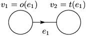
We consider a simple Abelian theory. Abelian gauge fields reside at vertices and scalar fields reside at edges. The $U(1)$ transformation is defined at each vertex. The Lagrangian density is

{\cal L}=-\frac{1}{4}\sum_{v\in V}F_{\mu\nu}^{v}F^{\mu\nu}_{v}-\sum_{e\in E}({\cal D}_{\mu}U_{e})^{\dagger}({\cal D}^{\mu}U_{e})\,,

(1)

where the covariant derivative is

{\cal D}^{\mu}U_{e}=(\partial^{\mu}+igA^{\mu}_{t(e)}-igA^{\mu}_{o(e)})U_{e}\,,

(2)

with $|U_{e}|^{2}=f^{2}$ .

If we rewrite $U_{e}$ as $U_{e}=f\,e^{ia_{e}}$ , the real scalar fields $a_{e}$ act as the Stueckelberg fields.[5] The number of physical massless scalar fields is $q-p+1$ , or the number of closed circuits involved in the graph, because $p-1$ scalar degrees of freedom are absorbed by the to-be massive vector fields. If and only if the graph is tree (or absent from closed circuits), the scalar fields disappear from the physical spectrum.

The $(mass)^{2}$ matrix of vector fields $M^{2}_{A}$ is given by $2g^{2}f^{2}\Delta$ , where the $(p,p)$ matrix

\Delta\equiv EE^{T}\,,

(3)

is called as the graph Laplacian and the $(p,q)$ matrix $E$ is the incidence matrix ¹¹ 1 Unfortunately, the symbol $E$ is used for the incidence matrix and for the set of edges. Please do not confuse them. defined as

(E)_{ve}=\left\{\begin{array}[]{cc}1&{\rm if~}v=o(e)\\ -1&{\rm if~}v=t(e)\\ 0&{\rm otherwise}\end{array}\right.\,.

(4)

Here $v=o(e)$ means that the vertex $v$ is the origin of the edge $e$ and $v=t(e)$ means that the vertex $v$ is the terminus of the edge $e$ . The $(q,p)$ matrix $E^{T}$ is the transposed matrix of $E$ .

For more general cases, one might consider individual coupling constants for vertices as

{\cal D}^{\mu}U_{e}=(\partial^{\mu}+ig_{t(e)}A^{\mu}_{t(e)}-ig_{o(e)}A^{\mu}_{o(e)})U_{e}\,,

(5)

and $|U_{e}|^{2}=f_{e}^{2}$ for each edge. In this case the mass matrix becomes

M^{2}_{A}=2GEF^{2}E^{T}G=2(GEF)(GEF)^{T},

(6)

where the diagonal matrices $G$ and $F$ are given by

(G)_{vv^{\prime}}=\left\{\begin{array}[]{cc}g_{v}&{\rm if~}v=v^{\prime}\\ 0&{\rm otherwise}\end{array}\right.\,,\quad(F)_{ee^{\prime}}=\left\{\begin{array}[]{cc}f_{e}&{\rm if~}e=e^{\prime}\\ 0&{\rm otherwise}\end{array}\right.\,,

(7)

respectively.

To summarize this section: In the GDD model, the mass spectrum is given by eigenvalues of the graph Laplacian or the related matrix constructed from the incidence matrix of the graph.

III The use of the Stueckelberg superfield

Next we incorporate SUSY into the GDD model. We use superfields [6] to this end.

In this paper, we consider that vector superfields $\{V_{v}\}$ exist on vertices. We still impose the $U(1)$ transformation on $V_{v}$ at each vertex as

V_{v}\rightarrow V_{v}+i(\Lambda_{v}-\overline{\Lambda}_{v})\,,

(8)

where $\Lambda_{v}$ is a chiral superfield. Then the invariant superfield is defined as usual: [6]

W_{\alpha}^{v}=-\frac{1}{4}\overline{D}\,\overline{D}\,D_{\alpha}{V_{v}}\,.

(9)

The kinetic term of the vector field can be created from this for each vertex.

Further we introduce a chiral superfield $S_{e}$ at each edge. The superfield $S_{e}$ is assumed to be transformed as:

{S_{e}}\rightarrow S_{e}-i\Lambda_{t(e)}+i\Lambda_{o(e)}\,.

(10)

Then we can write the Stueckelberg term [7]

(V_{t(e)}-V_{o(e)}+S_{e}+\overline{S}_{e})^{2}\,,

(11)

and a gauge invariant term for the interaction with scalars

\displaystyle{\cal L}

\displaystyle=

\displaystyle\sum_{v\in V}\frac{1}{4g_{v}^{2}}\left(\left.W^{\alpha}_{v}W^{v}_{\alpha}\right|_{\theta\theta}+\left.\overline{W}^{v}_{\dot{\alpha}}\overline{W}^{\dot{\alpha}}_{v}\right|_{\bar{\theta}\bar{\theta}}\right)+\sum_{e\in E}\,\left.2f_{e}^{2}(V_{t(e)}-V_{o(e)}+S_{e}+\overline{S}_{e})^{2}\right|_{\theta\theta\bar{\theta}\bar{\theta}}.

(12)

The bosonic part of the theory is found to be

	$\displaystyle{\cal L}_{b}$	$\displaystyle=$	$\displaystyle-\sum_{v\in V}\frac{1}{4g_{v}^{2}}F_{\mu\nu}^{v}F^{\mu\nu}_{v}-\sum_{e\in E}\frac{2f_{e}^{2}}{2}(A_{t(e)}^{\mu}-A_{o(e)}^{\mu}+\partial^{\mu}a_{e})^{2}-\frac{1}{2}\sum_{e\in E}2f_{e}^{2}(\partial^{\mu}\rho_{e})^{2}$		(13)
			$\displaystyle+\sum_{v\in V}\frac{1}{2g_{v}^{2}}D^{2}_{v}+2\sum_{e\in E}2f_{e}^{2}\|F_{Se}\|^{2}+\sum_{e\in E}2f_{e}^{2}(D_{t(e)}-D_{o(e)})\rho_{e}\,,$		(13)

where the notation of component field is rather standard one and is gathered in Appendix A.

Eliminating the auxiliary fields $F_{Se}$ and rescaling $\rho_{e}$ , gauge fields and $D_{v}$ to have canonical kinetic terms we get

	$\displaystyle{\cal L}_{b}$	$\displaystyle=$	$\displaystyle-\frac{1}{4}\sum_{v\in V}F_{\mu\nu}^{v}F^{\mu\nu}_{v}-\sum_{e\in E}\frac{2f_{e}^{2}}{2}(g_{t(e)}A_{t(e)}^{\mu}-g_{o(e)}A_{o(e)}^{\mu}+\partial^{\mu}a_{e})^{2}-\frac{1}{2}\sum_{e\in E}(\partial^{\mu}\rho_{e})^{2}$		(14)
			$\displaystyle-\sum_{e,e^{\prime}\in E}\sum_{v\in V}f_{e}\rho_{e}(E^{T})_{ev}g^{2}_{v}(E)_{ve^{\prime}}f_{e^{\prime}}\rho_{e^{\prime}}+\frac{1}{2}\sum_{v\in V}\left\{D_{v}-\frac{\sqrt{2}}{2}g_{v}\sum_{e\in E}(E)_{ve}f_{e}\rho_{e}\right\}^{2}.$		(14)

Now one can easily find the mass matrices for vectors and scalars:

M^{2}_{A}=2GEF^{2}E^{T}G=2(GEF)(GEF)^{T}\,,\quad M^{2}_{\rho}=2FE^{T}G^{2}EF=2(GEF)^{T}(GEF)\,,

(15)

where $E$ is defined as (4) while $G$ and $F$ are given by (7). Massless scalar fields are absent if and only if the graph is a tree graph. The mass spectrum of the scalar fields is the same as the one for the vector fields except for zero modes.²² 2 It is well known that two square matrices $AB$ and $BA$ have the same eigenvalues up to zero modes. See Appendix B.

The fermionic part of the theory is found to be

	$\displaystyle{\cal L}_{f}$	$\displaystyle=$	$\displaystyle-i\sum_{v\in V}\frac{1}{g_{v}^{2}}\lambda_{v}\sigma^{\mu}\partial_{\mu}\bar{\lambda}_{v}-i\sum_{e\in E}2f_{e}^{2}\chi_{e}\sigma^{\mu}\partial_{\mu}\bar{\chi}_{e}$		(16)
			$\displaystyle+\sum_{e\in E}2f_{e}^{2}\left[\chi_{e}(\lambda_{t(e)}-\lambda_{o(e)})+h.c.\right]\,,$		(16)

and can be rescaled as

	$\displaystyle{\cal L}_{f}$	$\displaystyle=$	$\displaystyle-i\sum_{v\in V}\lambda_{v}\sigma^{\mu}\partial_{\mu}\bar{\lambda}_{v}-i\sum_{e\in E}\chi_{e}\sigma^{\mu}\partial_{\mu}\bar{\chi}_{e}$		(17)
			$\displaystyle-\sum_{e\in E}\sum_{v\in V}\sqrt{2}\left[f_{e}\chi_{e}(E^{T})_{ev}g_{v}\lambda_{v}+h.c.\right].$		(17)

Here $\lambda_{v}$ and $\chi_{e}$ are Weyl spinor fields contained in $V_{v}$ and $S_{e}$ , respectively.

One will find the mass matrices for fermions after rescaling the fields:

M^{2}_{\lambda}=2GEF^{2}E^{T}G=2(GEF)(GEF)^{T}\,,\quad M^{2}_{\chi}=2FE^{T}G^{2}EF=2(GEF)^{T}(GEF).

(18)

Note that the fermions $\lambda$ and $\chi$ form Dirac fields for massive modes. Also note that all field contents are neutral as well as free from interactions.

IV multi-vector, multi-Higgs model

IV.1 general construction

We will construct the model that the symmetry $[U(1)]^{p}$ is spontaneously broken to $U(1)$ . Therefore we will not use the Stueckelberg fields but the Higgs fields.

As the model in the previous section, we consider vector superfields on vertices and suppose that $U(1)$ transformation is defined at each vertex. Moreover in the present case, we introduce a ‘bi-charged’ scalar field $\Sigma$ on each edge, which is transformed under two $U(1)$ symmetries as ³³ 3 Note that the transformation law for $\Sigma_{e}$ is the same as that for $e^{2S_{e}}$ in the previous section.,

\Sigma_{e}\rightarrow e^{-2i\Lambda_{t(e)}}\,\Sigma_{e}\,e^{2i\Lambda_{o(e)}}\,.

(19)

Now we get the $[U(1)]^{p}$ invariant supersymmetric multi-vector, multi-‘Higgs’ model on a graph governed by the following Lagrangian:

	$\displaystyle{\cal L}$	$\displaystyle=$	$\displaystyle\frac{1}{4}\sum_{v\in V}\left(\left.W^{\alpha}_{v}W^{v}_{\alpha}\right\|_{\theta\theta}+\left.\overline{W}^{v}_{\dot{\alpha}}\overline{W}^{\dot{\alpha}}_{v}\right\|_{\bar{\theta}\bar{\theta}}\right)+\sum_{e\in E}\,\left.\overline{\Sigma}_{e}\,e^{2gV_{t(e)}}\Sigma_{e}\,e^{-2gV_{o(e)}}\right\|_{\theta\theta\bar{\theta}\bar{\theta}}$		(20)
		$\displaystyle-$	$\displaystyle 2g\sum_{e\in V}\,\left.\zeta_{e}(V_{t(e)}-V_{o(e)})\right\|_{\theta\theta\bar{\theta}\bar{\theta}}\,,$		(20)

where we rescale the gauge coupling constant to be seen explicitly. The Fayet-Illiopoulos terms are chosen so that they are similar to those in the model of the previous section, when $\zeta_{e}\approx f_{e}^{2}$ .⁴⁴ 4 In most general cases, we can choose the Fayet-Illiopoulos (FI) terms as $\sim\sum_{v}\zeta_{v}V_{v}$ . We would like to study aspects of (gauge and/or super-) symmetry breakdown with the general FI terms elsewhere. This paper will not go into the issue about anomaly and deal with only classical aspects of the model.

The bosonic part of the Lagrangian reads

	$\displaystyle{\cal L}_{b}$	$\displaystyle=$	$\displaystyle-\frac{1}{4}\sum_{v\in V}F_{\mu\nu}^{v}F^{\mu\nu}_{v}+\frac{1}{2}\sum_{v\in V}D^{2}_{v}-\sum_{e\in E}({\cal D}_{\mu}\sigma_{e})^{\dagger}({\cal D}^{\mu}\sigma_{e})$		(21)
		$\displaystyle+$	$\displaystyle\sum_{e\in E}F^{\dagger}_{\Sigma\,e}F_{\Sigma\,e}+g\sum_{e\in E}(D_{t(e)}-D_{o(e)})\sigma^{\dagger}_{e}\sigma_{e}-g\sum_{e\in V}(D_{t(e)}-D_{o(e)})\zeta_{e}\,,$		(21)

where the covariant derivative is

{\cal D}^{\mu}\sigma_{e}=(\partial^{\mu}+igA^{\mu}_{t(e)}-igA^{\mu}_{o(e)})\sigma_{e}\,.

(22)

By use of the incidence matrix of the graph, we rewrite the above Lagrangian as

	$\displaystyle{\cal L}_{b}$	$\displaystyle=$	$\displaystyle-\frac{1}{4}\sum_{v\in V}F_{\mu\nu}^{v}F^{\mu\nu}_{v}+\frac{1}{2}\sum_{v\in V}D^{2}_{v}-\sum_{e\in E}({\cal D}_{\mu}\sigma_{e})^{\dagger}({\cal D}^{\mu}\sigma_{e})$		(23)
		$\displaystyle+$	$\displaystyle\sum_{e\in E}F^{\dagger}_{\Sigma\,e}F_{\Sigma\,e}-g\sum_{e\in E}(\sigma^{\dagger}_{e}\sigma_{e}-\zeta_{e})(E^{T}D)_{e}\,.$		(23)

Substituting the equation of motion for the auxiliary fields

F_{\Sigma\,e}=0\quad{\rm and}\quad D_{v}=g\sum_{e\in E}(\sigma^{\dagger}_{e}\sigma_{e}-\zeta_{e})(E^{T})_{v}\,,

(24)

into the bosonic Lagrangian, we obtain

	$\displaystyle{\cal L}_{b}$	$\displaystyle=$	$\displaystyle-\frac{1}{4}\sum_{v\in V}F_{\mu\nu}^{v}F^{\mu\nu}_{v}-\sum_{e\in E}({\cal D}_{\mu}\sigma_{e})^{\dagger}({\cal D}^{\mu}\sigma_{e})$		(25)
		$\displaystyle-$	$\displaystyle\frac{g^{2}}{2}\sum_{e,e^{\prime}\in E}(\sigma^{\dagger}_{e}\sigma_{e}-\zeta_{e})(E^{T}E)_{ee^{\prime}}(\sigma^{\dagger}_{e^{\prime}}\sigma_{e^{\prime}}-\zeta_{e^{\prime}})\,.$		(25)

Note that $E^{T}E$ is a $(q,q)$ matrix.

IV.2 example: $P_{3}$

The structure of the model depends on the incidence matrix of the graph. For a simple example, let us consider the path graph with three vertices, $P_{3}$ .

The incidence matrix depends on the orientation of edges. For instance, two cases can be considered as follows:⁵⁵ 5 Obviously the overall sign of the incidence matrix is irrelevant.

({E_{A}})_{ve}=\left(\begin{array}[]{cc}1&0\\ -1&1\\ 0&-1\end{array}\right)\,,\quad({E_{B}})_{ve}=\left(\begin{array}[]{cc}1&0\\ -1&-1\\ 0&1\end{array}\right)\,,

(26)

where $E_{A}$ is the incidence matrix of $P_{3}^{A}$ and $E_{B}$ is the one of $P_{3}^{B}$ .

Interestingly, the following matrix is independent of the edge orientation:

{E_{A}E_{A}^{T}}={E_{B}E_{B}^{T}}=\left(\begin{array}[]{ccc}1&-1&0\\ -1&2&-1\\ 0&-1&1\end{array}\right)\equiv\Delta\,.

(27)

This is known as the graph Laplacian.

On the other hand, we find

{E_{A}^{T}E_{A}}=\left(\begin{array}[]{cc}~2&-1\\ -1&~2\end{array}\right)\,,\quad{E_{B}^{T}E_{B}}=\left(\begin{array}[]{cc}~2&~1\\ ~1&~2\end{array}\right)\,.

(28)

Therefore the shape of the ‘Higgs’ potential in Eq. (25) depends on the edge orientation.

Figure 4 illustrates the contour plots of the potentials in Eq. (25) for the graphs $P^{A}_{3}$ and $P^{B}_{3}$ .

IV.3 mass matrices for bosonic and fermionic fields

Individually different gauge coupling constants will also be considered. The consequence of such consideration forces the bosonic part of the Lagrangian to be

	$\displaystyle{\cal L}_{b}$	$\displaystyle=$	$\displaystyle-\frac{1}{4}\sum_{v\in V}F_{\mu\nu}^{v}F^{\mu\nu}_{v}-\sum_{e\in E}({\cal D}_{\mu}\sigma_{e})^{\dagger}({\cal D}^{\mu}\sigma_{e})$		(29)
		$\displaystyle-$	$\displaystyle\frac{1}{2}\sum_{e,e^{\prime}\in E}\sum_{v\in V}(\sigma^{\dagger}_{e}\sigma_{e}-\zeta_{e})(E^{T})_{ev}g^{2}_{v}(E)_{ve^{\prime}}(\sigma^{\dagger}_{e^{\prime}}\sigma_{e^{\prime}}-\zeta_{e^{\prime}})\,,$		(29)

with

{\cal D}^{\mu}\sigma_{e}=(\partial^{\mu}+ig_{t(e)}A^{\mu}_{t(e)}-ig_{o(e)}A^{\mu}_{o(e)})\sigma_{e}\,.

(30)

Here we assume that all $\zeta_{e}$ are positive and $\sqrt{\zeta_{e}}=f_{e}$ . Thus the vacuum expectation value for $|\sigma_{e}|$ is $f_{e}$ and physical scalar fields should be considered as the linear combinations of $|\sigma_{e}|-f_{e}$ . Each phase part of a to-be massive scalar field is eaten by a vector field through the Higgs mechanism. Then the $(mass)^{2}$ matrices $M_{V}^{2}$ for vector fields and $M_{S}^{2}$ for scalar fields in this case are

M^{2}_{V}=2GEF^{2}E^{T}G=2(GEF)(GEF)^{T}\,,\quad M^{2}_{S}=2FE^{T}G^{2}EF=2(GEF)^{T}(GEF)\,,

(31)

where the matrices that appeared in the above equations are the same as (4) and (7).

Although the shape of the potential with respect to $|\sigma_{e}|$ depends on the orientation of edges in the graph, the mass spectrum of the scalar fields is the same as the one for the vector fields except for zero modes, similarly to the model in the previous section.

The number of the moduli of the potential is $q-p+1$ for a general graph. This is equal to the number of independent closed circuits in the graph.⁶⁶ 6 If $q-p+1>0$ , the graph has a closed circuit $C(G)$ . It is possible that we add the term like $\sum_{\{e_{1},e_{2},e_{3}\}\in C(G)}\Sigma_{e_{1}}\Sigma_{e_{2}}\Sigma_{e_{3}}$ to the Lagrangian to give the scalar masses. For tree graphs, the vacuum expectation values of $\sigma_{e}$ are determined rigidly if all $\zeta_{e}$ are positive.

The fermionic part of the Lagrangian is

	$\displaystyle{\cal L}_{f}$	$\displaystyle=$	$\displaystyle-i\sum_{v\in V}\lambda_{v}\sigma^{\mu}\partial_{\mu}\bar{\lambda}_{v}-i\sum_{e\in E}\psi_{e}\sigma^{\mu}{\cal D}_{\mu}\bar{\psi}_{e}$		(32)
		$\displaystyle+$	$\displaystyle i\sqrt{2}\sum_{e\in E}(\sigma_{e}\bar{\psi}_{e}(E^{T})_{ev}g_{v}\bar{\lambda}_{v}-\sigma_{e}^{\dagger}\psi_{e}(E^{T})_{ev}g_{v}\lambda)\,,$		(32)

where $\lambda_{v}$ and $\psi_{e}$ are Weyl spinor fields contained in $V_{v}$ and $\Sigma_{e}$ , respectively. The covariant derivative on $\psi_{e}$ is defined as ${\cal D}^{\mu}\psi_{e}=(\partial^{\mu}+ig_{t(e)}A^{\mu}_{t(e)}-ig_{o(e)}A^{\mu}_{o(e)})\psi_{e}$ . Substituting the vacuum expectation values $\langle\sigma_{e}\rangle=f_{e}$ , we find

M^{2}_{\lambda}=2(GEF)(GEF)^{T}\,,\quad M^{2}_{\psi}=2(GEF)^{T}(GEF)\,.

(33)

Since SUSY is unbroken, the bosonic and fermionic spectra are the same.

In this paper, we have considered models with unbroken SUSY. The model with ‘partially’ broken SUSY is interesting, for some $\zeta_{e}<0$ . The present analysis will not go into such models.

V vortex solution

It is well known that the vortex solution can be found in the Abelian-Higgs model [8]. In many papers, the solution is used as a simple model for a cosmic string [9]. We consider the vortex-type solutions in our model described in the previous section.

Although an academic interest in our toy model is an important motivation for the following study, we also think that topological configurations are a key ingredient in recent studies in theoretical physics. A possibility is expected that a similar model provides an example of a complicated brane/string system. In the present paper, anyway, we study only simple vortex in our theory and their generalizations and possible applications to particle physics and cosmology are left for future work.

Moreover we will consider only tree graphs as the bases of models.

V.1 Bogomolnyi equation

In the Abelian-Higgs model, the vortex solution is well known [8]. Moreover, it is known [10] that supersymmetric $U(1)$ theory satisfies the Bogomolnyi condition [11]. Because our model is also supersymmetric, the Bogomolnyi condition can be found. The equations of motion can be reduced to the following two sets of equations:

F^{ij}_{v}=\mp\varepsilon^{ij}g_{v}\sum_{e\in E}(E)_{ve}(|\sigma_{e}|^{2}-\zeta_{e})\,,

(34)

and

{\cal D}^{i}\sigma_{e}=\mp i\varepsilon^{ij}{\cal D}_{j}\sigma_{e}\,,

(35)

where $i,j$ denote two spatial directions and $\varepsilon^{ij}$ is the antisymmetric tensor.

These equations are the Bogomolnyi equations.

The energy per unit length of a vortex string can be written as

$\displaystyle{\cal E}$	$\displaystyle=$	$\displaystyle\int d^{2}x\left[\frac{1}{4}\sum_{v\in V}F_{ij}^{v}F^{ij}_{v}+\sum_{e\in E}({\cal D}_{i}\sigma_{e})^{\dagger}({\cal D}^{i}\sigma_{e})\right.$	(37)
		$\displaystyle\qquad\qquad+\left.\frac{1}{2}\sum_{e,e^{\prime}\in E}\sum_{v\in V}(\|\sigma_{e}\|^{2}-\zeta_{e})(E^{T})_{ev}g^{2}_{v}(E)_{ve^{\prime}}(\|\sigma_{e^{\prime}}\|^{2}-\zeta_{e^{\prime}})\right]$
	$\displaystyle=$	$\displaystyle\int d^{2}x\left[\frac{1}{4}\sum_{v\in V}\left\{F^{ij}_{v}\pm\varepsilon^{ij}g_{v}(E)_{ve}(\|\sigma_{e}\|^{2}-\zeta_{e})\right\}^{2}+\frac{1}{2}\sum_{e\in E}\left\|{\cal D}^{i}\sigma_{e}\pm i\varepsilon^{ij}{\cal D}_{j}\sigma_{e}\right\|^{2}\right.$
		$\displaystyle\qquad\qquad\pm\left.\left\{\sum_{v\in V}\sum_{e\in E}\frac{1}{2}\varepsilon_{ij}F^{ij}_{v}g_{v}(E)_{ve}\zeta_{e}-i\sum_{e\in E}\varepsilon^{ij}\partial_{i}(\sigma_{e}^{\dagger}{\cal D}_{j}\sigma_{e})\right\}\right].$

For a solution of finite energy density, ${\cal D}_{i}\sigma_{e}$ is equal to zero at spatial infinity. If the asymptotic behavior of $\sigma_{e}$ is expressed by the azimuthal angle $\varphi$ and an integer $n_{e}$ , i.e. $\sigma_{e}\rightarrow\sqrt{\zeta_{e}}e^{in_{e}\varphi}$ , the condition tells $(E^{T}g_{v}A_{i}^{v})_{e}\rightarrow n_{e}\partial_{i}\varphi$ , and then $\int d^{2}x\,(E^{T}\varepsilon_{ij}g_{v}F^{ij}_{v})_{e}=4\pi n_{e}$ . Therefore the energy density becomes

	$\displaystyle{\cal E}$	$\displaystyle=$	$\displaystyle\int d^{2}x\left[\frac{1}{4}\sum_{v\in V}\left\{F^{ij}_{v}\pm\varepsilon^{ij}g_{v}(E)_{ve}(\|\sigma_{e}\|^{2}-\zeta_{e})\right\}^{2}+\frac{1}{2}\sum_{e\in E}\left\|{\cal D}^{i}\sigma_{e}\pm i\varepsilon^{ij}{\cal D}_{j}\sigma_{e}\right\|^{2}\right]$		(38)
			$\displaystyle\pm 2\pi\sum_{e\in E}\|n_{e}\|\zeta_{e}\,.$		(38)

We deal with the lowest bound for the energy density read from this result. The vortex solution satisfying the Bogomolnyi equation (34,35) has the energy density $2\pi\sum_{e\in E}|n_{e}|\zeta_{e}$ .⁷⁷ 7 Because of the presence of many fields, non-Bogomolnyi configuration may have lower energy (i.e., the Bogomolnyi solution may correspond to a local minimum).

V.2 Bogomolnyi vortices and SUSY

It is well known that the SUSY is partially broken in the topological background fields. Here we briefly describe the pattern of SUSY breaking in our model. Notation is indebted in [6]. According to SUSY, the variations of the gauginos $\lambda_{e}$ are

\delta_{\epsilon}\lambda_{v}=i\epsilon D_{v}+\sigma^{\mu\nu}F_{v\,\mu\nu}\epsilon\,.

(39)

Using the Bogomolnyi equations (34), and assuming the vortex string lies in the third direction for simplicity, the above variations are rewritten as

\delta_{\epsilon}\lambda_{v}=\mp iF^{12}_{v}(1\pm\sigma^{3})\epsilon\,.

(40)

This means that the half of the SUSY at the vertex is broken in the presence of the central magnetic flux of the vortex.

The variations of partners of $\sigma_{e}$ are

\delta_{\epsilon}\psi_{e}=i\sqrt{2}\bar{\epsilon}\,\sigma^{\mu}{\cal D}_{\mu}\sigma_{e}\,,

(41)

where ${\cal D}^{\mu}\psi_{e}\equiv\partial^{\mu}\psi_{e}+i((gA)_{t(e)}^{\mu}-(gA)_{o(e)}^{\mu})\psi_{e}$ . If the vortex string lies in the third direction, this reduces when the Bogomolnyi equations (35) hold,

\delta_{\epsilon}\psi_{e}=i\sqrt{2}\bar{\epsilon}\,\left[\sigma^{1}{\cal D}_{1}\psi_{e}+\sigma^{2}{\cal D}_{2}\psi_{e}\right]=i\sqrt{2}\bar{\epsilon}\,(\sigma^{1}\pm i\sigma^{2}){\cal D}_{1}\psi_{e}\,.

(42)

We find again that the half of the SUSY at the edge is broken in the presence of the magnetic flux.

V.3 construction of vortices: ansatz

Next we examine how we can obtain the explicit solutions in our model. For simplicity, we consider a common gauge coupling constant $g$ and a single constant $f=\sqrt{\zeta}$ . In other words, we consider the case that $G=gI$ and $F=fI$ (where $I$ is the identity matrix). Although we cannot tell about most general solutions, we take ansatz for simple, physically admissible type of vortex solutions.⁸⁸ 8 For a reference, we write down the construction of normal vortex solutions in Appendix C. We impose the axially symmetric ansatz

		$\displaystyle\sigma_{e}=\rho_{e}(r)\,e^{in_{e}\varphi}\,,$		(43)
		$\displaystyle A^{v}_{\varphi}=P_{v}(r)\,,$		(44)

on Bogomolnyi equations. Here we express the radial coordinate as $r$ and the azimuthal angle as $\varphi$ . The integers $n_{e}$ are winding numbers. The detailed calculation is shown in the Appendix D. We get the following Bogomolnyi equations,

		$\displaystyle\dfrac{\rho_{e}^{\prime}}{\rho_{e}}=-\dfrac{\left(g\left(E^{T}P\right)-n\right)_{e}}{r}\,,$		(45)
		$\displaystyle\dfrac{P_{v}^{\prime}}{r}=-g\sum_{e\in E}\left(E\right)_{ve}\left(\rho^{2}-f^{2}\right)_{e}\,,$		(46)

where the prime (^′) denotes the derivative with respect to $r$ . These equations are the special case of the Bogomolnyi equations.

V.4 examples of vortex solutions

We show some concrete examples for the vortex solution in our model. To have the vortex solution we restrict the graph structure, or equivalently, the incident matrix $E$ . Here we also consider configurations with the least winding numbers for simplicity and for feasibility in physical systems.

We consider here the cases with the single-centered exact solution similar to the normal vortex. The asymptotic behavior of general cases can be obtained and is shown in Appendix E.

V.4.1 Example 1: $P_{2}$

The simplest case has two vertices and an edge. This graph is $P_{2}$ graph. We show the graph in FIG. 5.

In this case, the incidence matrix and its transposed matrix are

(E)_{ve}=\begin{pmatrix}1\\ -1\\ \end{pmatrix},\ \ \ \ \left(E^{T}\right)_{ev}=\begin{pmatrix}1&-1\\ \end{pmatrix}\,.

(47)

Then considering the Bogomolnyi equations

	$\displaystyle\dfrac{P_{v}^{\prime}}{r}$	$\displaystyle=-g\sum_{e\in E}(E)_{ve}\left(\rho^{2}-f^{2}\right)_{e}\,,$		(48)
	$\displaystyle\dfrac{\rho_{e}^{\prime}}{\rho_{e}}$	$\displaystyle=-\dfrac{\left(g\,E^{T}P-n\right)_{e}}{r}\,,$		(49)

the first one becomes

	$\displaystyle\dfrac{P_{1}^{\prime}}{r}$	$\displaystyle=-g\left(\rho^{2}-f^{2}\right)\,,$		(50)
	$\displaystyle\dfrac{P_{2}^{\prime}}{r}$	$\displaystyle=+g\left(\rho^{2}-f^{2}\right)\,.$		(51)

Therefore it is necessary to find a set of unique equations that we suppose the relation $P_{1}(r)=-P_{2}(r)$ . On the other hand, in the second equation we notice

\sum_{v}(E^{T})_{ev}P_{v}=\begin{pmatrix}1&-1\\ \end{pmatrix}\begin{pmatrix}1\\ -1\\ \end{pmatrix}P_{1}=2P_{1}\,.

(52)

So, we get the following equations

	$\displaystyle\dfrac{P_{1}^{\prime}}{r}$	$\displaystyle=-g\left(\rho^{2}-f^{2}\right)\,,$		(53)
	$\displaystyle\dfrac{\rho^{\prime}}{\rho}$	$\displaystyle=-\dfrac{2gP_{1}-n}{r}\,.$		(54)

These equations can be reduced to

	$\displaystyle\dfrac{\tilde{P}^{\prime}}{x}$	$\displaystyle=-\left(\tilde{\rho}^{2}-1\right)\,,$		(55)
	$\displaystyle\dfrac{\tilde{\rho}^{\prime}}{\tilde{\rho}}$	$\displaystyle=-\dfrac{\tilde{P}-n}{x}\,,$		(56)

if we rescale the variables so that $\tilde{P}(x)=2gP_{1}(r)$ , $\tilde{\rho}(x)={\rho}(r)/{f}$ , $x=\sqrt{2}gfr$ , $n=1$ and the prime (^′) is the derivative with respect to $x$ . These equations are precisely same as the normal Bogomolnyi equations. The normal Bogomolnyi equations is referred in Appendix C.

The energy per unit length of the straight string is given by $2\pi f^{2}$ in this case. Generalization to the case with the winding number $n>1$ is trivial.

V.4.2 Example 2: $P_{3}$

We consider the $P_{3}$ graph, the three-vertex path graph. In this graph, we consider two patterns of the direction of the edges. We show these in FIG. 6.

The condition to reduce the Bogomolnyi equations in these cases to the normal ones (55,56) with $\rho_{1}=\rho_{2}$ and $n_{1}=n_{2}=1$ are $P_{1}(r)=-P_{3}(r)$ and $P_{2}(r)\equiv 0$ in the case with $P_{3}^{A}$ while $P_{1}(r)=P_{3}(r)$ and $P_{2}(r)=-2P_{1}(r)$ in the case with $P_{3}^{B}$ . The necessary scaling is that $\tilde{P}(x)=gP_{1}(r)$ and $x=gfr$ in the case with $P_{3}^{A}$ while $\tilde{P}(x)=3gP_{1}(r)$ and $x=\sqrt{3}gfr$ in the case with $P_{3}^{B}$ . The energy density takes the same value $2\pi f^{2}(1+1)=4\pi f^{2}$ in both cases.

V.4.3 Example 3: $K_{1,N}$

We consider another tree graph, the star graph $K_{1,N}$ . In the star graph, $v_{N+1}$ is adjacent to all the other vertices and no extra edge exists. We recognize two types of edges. One is the edge whose origin is $v_{N+1}$ , another edge is one whose terminus is $v_{N+1}$ . We call the edge of the first type is $e_{o}$ , the one of the second type is $e_{t}$ .

We heuristically find the cases that we get the vortex solution similar to the normal one with $\rho_{1}=\rho_{2}=\cdots=\rho_{N}=\rho_{N+1}$ : Here two cases are shown where the number of edges belonging to two types are

	$\displaystyle K_{1,N}^{A}:\quad$	$\displaystyle\#e_{o}=\#e_{t}=N/2\,,$		(57)
	$\displaystyle K_{1,N}^{B}:\quad$	$\displaystyle\#e_{o}=N\quad{\rm and}\quad\ \#e_{t}=0\,,~or~vice~versa\,,$		(58)

where, off course, $N$ is considered to be even in the case $A$ . The graphs of two types are shown in FIG. 7.

The incidence matrix of $K^{A}_{1,N}$ (where $N$ is even) is $(N+1,N)$ matrix given by

(E_{A})_{ve}=\left(\begin{array}[]{ccccccc}-1&0&0&\cdots&0\\ 0&1&0&\cdots&0\\ 0&0&-1&\cdots&0\\ \vdots&\vdots&\vdots&\ddots&\vdots\\ 0&0&0&\cdots&1\\ 1&-1&1&\cdots&-1\end{array}\right)\,,

(59)

while the incidence matrix of $K^{B}_{1,N}$ is

(E_{B})_{ve}=\left(\begin{array}[]{ccccccc}-1&0&0&\cdots&0\\ 0&-1&0&\cdots&0\\ 0&0&-1&\cdots&0\\ \vdots&\vdots&\vdots&\ddots&\vdots\\ 0&0&0&\cdots&-1\\ 1&1&1&\cdots&1\end{array}\right)\,.

(60)

We found these patterns by extending the analysis of getting the vortex solution in the case with $P_{3}$ graph shown previously, because $K_{1,2}$ is the same as $P_{3}$ .

In the first case (57), we have vortex solutions if $P_{2\ell-1}(r)=-P_{2m}(r)$ ( $\ell,m$ are positive integers and $\ell,m\leq\frac{N}{2}$ ) and $P_{N+1}\equiv 0$ . In the second case (58), we have the solutions if $P_{1}(r)=P_{2}(r)=\cdots=P_{N}(r)$ and $P_{N+1}(r)=-NP_{1}(r)$ . In both cases the energy density is found to be $2\pi Nf^{2}$ if all the winding numbers are unity.

V.4.4 Inclusion of ‘no winding scalar edge’

In the previous two examples, all ‘Higgs’ scalars have nonzero winding number. Conversely we consider that there is an edge where the assigned scalar has no winding number, thus $\rho_{e}\equiv f$ at the edge. We use the dashed line to express such an edge, as in FIG. 8.

For a constant $\rho_{e}$ , $P_{o(e)}(r)\equiv P_{t(e)}(r)$ holds everywhere.⁹⁹ 9 Thus the orientation of the edge is irrelevant (so, there is no arrow assigned to the dashed line). Suppose that one have already constructed the vortex solution in a certain model with specific graph structure. The one might duplicate the solution and the graph. One may connect the identical vertices of the original and copy of the graph by ‘no winding scalar edge’. The number of such connection is arbitrary. This method can be applied to the case with two different models and solutions, if one finds the same functional form of $P_{v}(r)$ in each model. Of course more than two vertices can be connected if $P_{v}$ is common at all vertices.

V.4.5 Example 4: $P_{4}$

We consider the $P_{4}$ graph. The graph $P_{4}$ has two $P_{2}$ as subgraphs and is shown in FIG. 9. We do not show the direction of the edge in this graph. This graph has a left-right symmetry with respect to the dashed edge. This symmetry is connected with the winding number of each vector fields. The vector fields at the both ends of the dashed line must be described by an identical function. For this reason, we should impose the left-right symmetry to the direction of edges. In the $P_{4}$ case, we find two types of the edge orientation graph for admitting the normal vortex solutions, shown in FIG. 10 and FIG. 11.

In the similar way, we consider the model based on $P_{2\ell}$ with normal vortex solutions.

V.4.6 Example 5: $P_{6}$

The graph $P_{6}$ has three $P_{2}$ as subgraphs. We study the model based on $P_{6}$ and their standard solution in the above-mentioned way.

In addition, $P_{6}$ has two $P_{3}$ as subgraphs. Similarly to the case with $P_{4}$ , we can consider the $P_{6}$ graph as two subgraphs connected by an edge. We exhibit the $P_{6}$ graph in FIG. 12. We have the left-right symmetry with respect to the dashed edge also in this case. We classify four types of the graph in terms of the direction of the edges as in FIG. 13.

In the similar way, we can consider the $P_{3\ell}$ graph, and associated models and solutions.

V.4.7 Example 6

We can connect two $K_{1,N}$ graphs by the dashed edge as in FIG. 14.

As this example, we can find the graph structure admitting the normal vortex solutions.

VI Conclusion and Outlook

We have generalized DD into GDD and introduced SUSY to GDD in the Abelian theory. A multi-Abelian-Higgs model has been studied as a further generalization. After getting the Bogomolnyi equations, we explicitly constructed vortex solutions of the normal type. To get the vortex solution, we restricted the graph structure to the special cases shown in the previous section. We showed some examples for the graph which has the normal vortex solution.

We have left the following aspects of the multi-Abelian-Higgs models for future work. First, we discussed single-centered vortex in the present paper. The possibility of multi-vortex solution [12] is an important subject to study. Next, in this paper, we mainly considered tree graphs. If we take general graph structures as the bases of multi-Abelian-Higgs models, we have scalar potentials with (many) flat direction of the lowest energy. The appearance of moduli is the feature of supersymmetric theories and the vortex solution in such a model is crucial for phenomenological models [13]. At the same time, the quantum corrections might become essential. The generalization of the method in [14] will be useful to investigate the quantum effects about vortices. Finally, because our model contains several fields, the possibility of different types of topological defects, such as ‘rings’ [15], must be examined.

We considered the Abelian gauge theory in GDD as well as multi-Higgs models. We are also interested in the non-Abelian theory because the three-site Higgsless model is based on the $[SU(2)]^{2}\otimes U(1)$ gauge theory. While we considered vortices in the Abelian gauge theory in this paper, on the other hand there exist monopoles in the non-Abelian gauge theory. As the future works, we wish to incorporate monopoles, superfields and GDD into non-Abelian theory as some toy models for the Higgsless model.

Acknowledgement

We would like to thank T. Hanada for useful comments.

Appendix A contents of superfields

In this Appendix, we collect the superfields and their component fields. See the reference [6].

A.1 vector superfield

V_{v}=-\theta\sigma_{\mu}\bar{\theta}A^{\mu}_{v}+i\theta\theta\bar{\theta}\bar{\lambda}_{v}-i\bar{\theta}\bar{\theta}\theta\lambda_{v}+\frac{1}{2}\theta\theta\bar{\theta}\bar{\theta}D_{v}\,.

(61)

This satisfies

V_{v}^{2}=-\frac{1}{2}\theta\theta\bar{\theta}\bar{\theta}A_{\mu}^{v}A^{\mu}_{v}\,,\quad V_{v}^{3}=0\,.

(62)

A.2 chiral superfield (Stueckelberg superfield)

	$\displaystyle S_{e}$	$\displaystyle=$	$\displaystyle\frac{1}{2}(\rho_{e}+ia_{e})+\theta\chi_{e}+i\theta\sigma^{\mu}\bar{\theta}\frac{1}{2}(\partial_{\mu}\rho_{e}+i\partial_{\mu}a_{e})$		(63)
			$\displaystyle+\theta\theta F_{Se}+\frac{i}{2}\theta\theta\bar{\theta}\bar{\sigma}^{\mu}\partial_{\mu}\chi_{e}+\frac{1}{8}\theta\theta\bar{\theta}\bar{\theta}(\rho_{e}+ia_{e})\,,$		(63)

	$\displaystyle S_{e}+\overline{S}_{e}$	$\displaystyle=$	$\displaystyle\rho_{e}+\theta\chi_{e}+\bar{\theta}\bar{\chi}_{e}-\theta\sigma^{\mu}\bar{\theta}\partial_{\mu}a_{e}+\theta\theta F_{Se}+\bar{\theta}\bar{\theta}F^{\dagger}_{Se}$		(64)
			$\displaystyle+\frac{i}{2}\theta\theta\bar{\theta}\bar{\sigma}^{\mu}\partial_{\mu}\chi_{e}+\frac{i}{2}\bar{\theta}\bar{\theta}\theta\sigma^{\mu}\partial_{\mu}\bar{\chi}_{e}+\frac{1}{4}\theta\theta\bar{\theta}\bar{\theta}\rho_{e}\,.$		(64)

A.3 chiral superfield (Higgs superfield)

	$\displaystyle\Sigma_{e}$	$\displaystyle=$	$\displaystyle\sigma_{e}+\sqrt{2}\theta\psi_{e}+i\theta\sigma^{\mu}\bar{\theta}\partial_{\mu}\sigma_{e}$		(65)
			$\displaystyle+\theta\theta F_{\Sigma e}+\frac{i}{\sqrt{2}}\theta\theta\bar{\theta}\bar{\sigma}^{\mu}\partial_{\mu}\psi_{e}+\frac{1}{4}\theta\theta\bar{\theta}\bar{\theta}(\sigma_{e})\,.$		(65)

Appendix B The eigenvalues of matrices $AB$ and $BA$

Let $A$ be a $(p,q)$ matrix and $B$ be a $(q,p)$ matrix. Then $(p+q,p+q)$ matrices $U$ and $V$ are defined as

U=\left(\begin{array}[]{cc}I_{p}&A\\ B&xI_{q}\end{array}\right)\,,\quad V=\left(\begin{array}[]{cc}xI_{p}&-A\\ 0_{qp}&I_{q}\end{array}\right)\,,

(66)

where $I_{p}$ is the $(p,p)$ identity matrix while $0_{qp}$ is the $(q,p)$ matrix all of which elements are zero.

The products of two matrices are

UV=\left(\begin{array}[]{cc}xI_{p}&0_{pq}\\ xB&xI_{q}-BA\end{array}\right)\,,\quad VU=\left(\begin{array}[]{cc}xI_{p}-AB&0_{pq}\\ B&xI_{q}\end{array}\right)\,.

(67)

Because $\det UV=\det VU$ , the eigenvalues of $AB$ and $BA$ are equal, except for zero eigenvalues.

Appendix C The normal vortex in Abelian-Higgs model

The Ginzburg-Landau theory is used as a macroscopic theory of the superconductivity. That is nonrelativistic theory, and we know an Abelian-Higgs model as the relativistic version of the Ginzburg-Landau theory. This model includes the normal vortex solution. In this paper we distinguish the vortex solution of the Abelian-Higgs model from the vortex solutions of our multi-Abelian-Higgs models, by using the word “normal”.

In the Abelian-Higgs model, the Lagrangian density is

\mathcal{L}=-\dfrac{1}{4}F^{\mu\nu}F_{\mu\nu}-\left|D_{\mu}\sigma\right|^{2}-\dfrac{1}{2}g^{2}\left(\sigma^{2}-f^{2}\right)^{2}\,,

(68)

where $F_{\mu\nu}=\partial_{\mu}A_{\nu}-\partial_{\nu}A_{\mu}$ is a field strength of the Abelian gauge field $A_{\mu}$ , $\sigma$ is a complex scalar field and $f$ is its vacuum expectation value $\langle\sigma\rangle=f$ . $D_{\mu}\sigma$ is the covariant derivative of the scalar field

D_{\mu}\sigma=\partial_{\mu}\sigma+igA_{\mu}\sigma,

(69)

where $g$ is the gauge coupling constant to the scalar field $\sigma$ .

To obtain the classical solution in this theory, we impose the static, axially-symmetric ansatz:

	$\displaystyle\bm{A}$	$\displaystyle=\bm{e}_{\varphi}P(r)\,,$		(70)
	$\displaystyle\sigma$	$\displaystyle=\rho(r)e^{in\varphi}\,,$		(71)

where the integer $n$ is the winding number. We used the circular cylindrical coordinates $r$ , $\varphi$ , and $z$ .

We use the scale conversion $x\equiv gfr$ , $\tilde{P}\equiv gP$ and $\tilde{\rho}\equiv\rho/f$ . Therefore the energy density of per unit length of the $z$ axis becomes

{\cal E}=2\pi f^{2}\int^{\infty}_{0}dx\ x\left[\dfrac{1}{2}\left(\dfrac{\tilde{P}^{\prime}}{x}+\tilde{\rho}^{2}-1\right)^{2}+\left(\tilde{\rho}^{\prime}+\dfrac{\tilde{P}-n}{x}\tilde{\rho}\right)^{2}-\dfrac{\tilde{P}^{\prime}}{x}\left(\tilde{\rho}^{2}-1\right)-2\tilde{\rho}\tilde{\rho}^{\prime}\dfrac{\tilde{P}-n}{x}\right],

(72)

where the prime (^′) denotes the derivative with respect to $x$ . Asymptotic values are as follows: $\tilde{P}(0)=0$ , $\tilde{P}(\infty)=n$ , $\tilde{\rho}(0)=0$ and $\tilde{\rho}(\infty)=1$ . We can write the following inequality for the energy

{\cal E}\geq 2\pi nf^{2}\int^{\infty}_{0}\left(\tilde{\rho}^{2}\right)^{\prime}dx=2\pi nf^{2}.

(73)

This lower bound on the energy is the Bogomolnyi bound and it is saturated when $\tilde{\rho}$ and $\tilde{P}$ satisfy the following equations

	$\displaystyle\dfrac{\tilde{P}^{\prime}}{x}$	$\displaystyle=-\left(\tilde{\rho}^{2}-1\right),$		(74)
	$\displaystyle\dfrac{\tilde{\rho}^{\prime}}{\tilde{\rho}}$	$\displaystyle=-\dfrac{\tilde{P}-n}{x}.$		(75)

These equations are the Bogomolnyi equations.

Appendix D Action and equation of motion with vortex ansatz

In this Appendix, we show the details about the Bogomolnyi equations for the vortex configuration. We take the axially symmetric ansatz:

\sigma_{e}=\rho_{e}(r)e^{in_{e}\varphi}\,,\quad A_{\varphi}^{v}=P_{v}(r)\,.

(76)

Then we find

{\cal D}_{r}\sigma_{e}=\rho^{\prime}_{e}e^{in_{e}\varphi}\,,\quad{\cal D}_{\varphi}\sigma_{e}=i(n_{e}+(gP)_{t(e)}-(gP)_{o(e)})\rho_{e}e^{in_{e}\varphi}\,,

(77)

where the prime denotes $\frac{d}{dr}$ , the derivative with respect to $r$ , and $(gP)_{v}=g_{v}P_{v}$ . Thus the kinetic term of the scalar reads

|{\cal D}_{i}\sigma_{e}|^{2}=(\rho^{\prime}_{e})^{2}+\frac{(n_{e}+(gP)_{t(e)}-(gP)_{o(e)})^{2}}{r^{2}}\rho_{e}^{2}\,,

(78)

while the Maxwell term becomes

\frac{1}{4}F_{v}^{ij}F_{ij}^{v}=\frac{1}{2}\frac{(P^{\prime}_{v})^{2}}{r^{2}}\,.

(79)

The total action can be rewritten as

	$\displaystyle{\cal E}$	$\displaystyle=$	$\displaystyle 2\pi\int_{0}^{\infty}dr\,r\left[\frac{1}{2}\sum_{v\in V}\frac{(P^{\prime}_{v})^{2}}{r^{2}}+\sum_{e\in E}\left\{(\rho^{\prime}_{e})^{2}+\frac{((E^{T}GP)_{e}-n_{e})^{2}}{r^{2}}\rho_{e}^{2}\right\}\right.$		(80)
			$\displaystyle\qquad\qquad\qquad+\left.\frac{1}{2}\sum_{e,e^{\prime}\in E}(\rho_{e}^{2}-\zeta_{e})(E^{T}G^{2}E)_{ee^{\prime}}(\rho_{e^{\prime}}^{2}-\zeta_{e^{\prime}})\right]\,,$		(80)

and this is no other than the energy density per unit length in the present static case.

Varying this, we obtain the following equations of motion:

	$\displaystyle\frac{(r\rho^{\prime}_{e})^{\prime}}{r}$	$\displaystyle=$	$\displaystyle\frac{((E^{T}GP)_{e}-n_{e})^{2}}{r^{2}}\rho_{e}+\sum_{e,e^{\prime}\in E}\rho_{e}(E^{T}G^{2}E)_{ee^{\prime}}(\rho_{e^{\prime}}^{2}-\zeta_{e^{\prime}})\,,$		(81)
	$\displaystyle\left(\frac{P^{\prime}_{v}}{r}\right)^{\prime}$	$\displaystyle=$	$\displaystyle 2\sum_{e\in E}\frac{((E^{T}GP)_{e}-n_{e})}{r^{2}}\rho_{e}^{2}(E^{T}G)_{ev}\,.$		(82)

These second-order simultaneous equations can be reduced to the first-order Bogomolnyi equations:

	$\displaystyle\rho^{\prime}_{e}$	$\displaystyle=$	$\displaystyle\mp\frac{(E^{T}GP)_{e}-n_{e}}{r}\rho_{e}\,,$		(83)
	$\displaystyle\frac{P^{\prime}_{v}}{r}$	$\displaystyle=$	$\displaystyle\mp\sum_{e\in E}(\rho_{e}^{2}-\zeta_{e})(E^{T}G)_{ev}\,.$		(84)

Appendix E asymptotic profile of the vortex

We investigate the asymptotic behavior of the solution of (83,84) in this Appendix. To this purpose, first we introduce new variables $p_{v}(r)$ and $R_{e}(r)$ :

P_{v}(r)=a_{v}-p_{v}(r)\,,\quad\rho_{e}=f_{e}-R_{e}(r)\,,

(85)

where the constant $a_{v}$ satisfies

n_{e}=(E^{T}Ga)_{e}\,.

(86)

Next we prepare $p$ -dimensional eigenvectors $x^{(a)}$ ( $a=1,\cdots,p-1$ ) for the $(mass)^{2}$ mass matrix for vector fields satisfying

2(GEF)(GEF)^{T}x^{(a)}=(m^{(a)})^{2}x^{(a)}\,,\quad{\rm for~nonzero~modes}

(87)

and $q$ -dimensional eigenvectors $X^{(a)}$ for the $(mass)^{2}$ mass matrix for scalar fields satisfying

2(GEF)^{T}(GEF)X^{(a)}=(m^{(a)})^{2}X^{(a)}\,.

(88)

Hereafter we restrict ourselves on the case with tree graphs treated in the text. Thus $q=p-1$ . The zero mode satisfies

2(GEF)(GEF)^{T}x^{(0)}=0\,.

(89)

The relations of two sets of eigenvectors are

X^{(a)}=\frac{\sqrt{2}}{m^{(a)}}(GEF)^{T}x^{(a)}\,,\quad x^{(a)}=\frac{\sqrt{2}}{m^{(a)}}GEFX^{(a)}\,,\quad(a\neq 0)

(90)

and we adopt the normalization convention:

x^{(a)T}x^{(a)}=X^{(a)T}X^{(a)}=1\,.

(91)

Using the eigensystems, we can expand the variables by eigenvectors as

p_{v}(r)=\sum_{(a)}p^{(a)}x^{(a)}_{v}\,,\quad R_{e}(r)=\sum_{(a)}R^{(a)}X^{(a)}_{e}\,,

(92)

Noticing $R_{e}(\infty)=0$ and $p_{v}(\infty)=0$ , the equations of motion (81,82) becomes at the asymptotic region, $r\rightarrow\infty$ ,

{R^{(a)}}^{\prime\prime}+\frac{1}{r}{R^{(a)}}^{\prime}-(m^{(a)})^{2}{R^{(a)}}=0\,,

(93)

{p^{(a)}}^{\prime\prime}-\frac{1}{r}{p^{(a)}}^{\prime}-(m^{(a)})^{2}{p^{(a)}}=0\,,

(94)

and the Bogomolnyi equations (83,84) become at the asymptotic region, $r\rightarrow\infty$ ,

{R^{(a)}}^{\prime}=-\frac{1}{r}\frac{m^{(a)}}{\sqrt{2}}{p^{(a)}}\,,

(95)

\frac{{{p^{(a)}}^{\prime}}}{r}=-\sqrt{2}m^{(a)}{R^{(a)}}\,.

(96)

The solution of the above equations is

R^{(a)}=C\,K_{0}(m^{(a)}r)\,,\quad p^{(a)}=\sqrt{2}C\,rK_{1}(m^{(a)}r)\,.

(97)

This result can be derived by using the following formulas for the modified Bessel function of the second type, such as $K_{0}(z)$ and $K_{1}(z)$ ;

K_{0}^{\prime\prime}(z)+\frac{1}{z}K_{0}^{\prime}(z)-K_{0}(z)=0\,,\qquad K_{1}^{\prime\prime}(z)+\frac{1}{z}K_{1}^{\prime}(z)-\left(1+\frac{1}{z^{2}}\right)K_{1}(z)=0\,,

(98)

(zK_{1}(z))^{\prime\prime}-\frac{1}{z}(zK_{1}(z))^{\prime}-(zK_{1}(z))=0\,,

(99)

K_{0}^{\prime}(z)=-K_{1}(z)\,,\qquad(zK_{1}(z))^{\prime}=-zK_{0}(z)\,,

(100)

where the prime (^′) means the derivative with respect to $z$ .

More rough estimation can be done with the exponential function because

K_{\nu}(z)\approx\sqrt{\frac{\pi}{2z}}e^{-z}\,,\quad{\rm for~large~}z\,.

(101)

References

[1] C. Csaki, C. Grojean, H. Murayama, L. Pilo and J. Terning, Phys. Rev. D69 (2004) 055006 [arXiv:hep-ph/0305237]. R. Foadi, S. Gopalakrishna and C. Schmidt, JHEP 0403 (2004) 042 [arXiv:hep-ph/0312324]. R. Sekhar Chivukula, H.-J. He, M. Kurachi, E. H. Simmons, M. Tanabashi, Phys. Rev. D71 (2005) 035007 [arXiv:hep-ph/0410154].
[2] R. Sekhar Chivukula, B. Coleppa, S. Di Chiara, E. H. Simmons, H. J. He, M. Kurachi and M. Tanabashi, Phys. Rev. D74 (2006) 075011 [arXiv:hep-ph/0607124], and references therein.
[3] N. Arkani-Hamed, A. G. Cohen and H. Georgi, Phys. Lett. B513 (2001) 232 ; N. Arkani-Hamed, A. G. Cohen and H. Georgi, Phys. Rev. Lett 86 (2001) 4757; C. T. Hill, S. Pokorski and J. Wang, Phys. Rev. D64 (2001) 105005.
[4] N. Kan and K. Shiraishi, J. Math. Phys. 46 (2005) 112301.
[5] For a review, see H. Ruegg and M. Ruiz-Altaba, Int. J. Mod. Phys. A19 (2004) 3265 [arXiv:hep-th/0304245].
[6] I. L. Buchbinder and S. M. Kuzenko, Ideas and Methods of Supersymmetry and Supergravity Or a Walk Through Superspace (IOP, Bristol, Revised edition 1998).
[7] S. V. Kuzmin and D. G. C. McKeon, Mod. Phys. Lett. A17 (2002) 2605 hep-th/0211166; B. Körs and P. Nath, JHEP 0507 (2005) 069 hep-ph/0503208; T. Kawano, Prog. Theor. Phys. 120 (2008) 793 arXiv:0712.2351[hep-th].
[8] H. J. de Vega and F. A. Schaposnik, Phys. Rev. D14 (1976) 1100. F. A. Schaposnik, hep-th/0611028.
[9] A. Vilenkin and E. P. S. Shellard, Cosmic Strings and Other Topological Defects (Cambridge Univ. Press, Cambridge, 1994).
[10] J. D. Edelstein, C. Núñez and F. A. Schaposnik, Phys. Lett. B329 (1994) 39; hep-th/9311055.
[11] E. B. Bogomolnyi, Sov. J. Nucl. Phys. 24 (1976) 449.
[12] E. J. Weinberg, Phys. Rev. D19 (1979) 3008. C. H. Taubes, Commun. Math. Phys. 72 (1980) 277.
[13] A. Achúcarro, A. C. Davis, M. Pickles and J. Urrestilla, Phys. Rev. D66 (2002) 105013; Phys. Rev. D68 (2003) 065006. Y. Cui, S. P. Martin, D. E. Morrissey and J. D. Wells, Phys. Rev. D77 (2008) 043528.
[14] A. Rebhan, P. van Nieuwenhuizen and R. Wimmer, Nucl. Phys. B679 (2004) 382; Braz. J. Phys. 34 (2004) 1273. A. S. Goldhaber, A. Rebhan, P. van Nieuwenhuizen and R. Wimmer, Phys. Rep. 398 (2004), 179.
[15] C. G. Doudoulakis, Physica D228 (2007) 159; Physica D234 (2007) 1;