Holographic superconductors are a class of quantum critical theories which have an instability to a superconducting phase at low temperatures when held at a finite chemical potential $\mu$ [17, 18, 19]. One can equivalently work with a fixed charge density $\rho$. Scale invariance and dimensional analysis imply that the critical temperature $T_{c}\propto\mu$. Our objective is to show that a large number of simple string vacua are holographic superconductors and to determine $T_{c}/\mu$ for these theories.

The minimal bulk action for a holographic superconductor must describe the dynamics of the metric, a Maxwell field and at least one charged field that can condense and spontaneously break the $U(1)$ symmetry. We focus in this work on the case in which the charged field is a scalar in $AdS_{4}$. In general the full nonlinear action is complicated, as a consistent embedding into string theory will typically involve many coupled fields. Physically this implies that there will be many condensates at low temperature. In this work we avoid this problem by only considering the scalar equations of motion to linearised order, at which many fields decouple. This is sufficient to determine the critical temperature.

The bulk action for a minimally coupled scalar field to quadratic order in the scalar is

$${\mathcal{L}}=\frac{M^{2}}{2}R+\frac{3M^{2}}{L^{2}}-\frac{1}{4g^{2}}F_{\mu\nu}F^{\mu\nu}-\left|\nabla\phi-iqA\phi\right|^{2}-m^{2}\left|\phi\right|^{2}\,.$$

(1)

There are four dimensionless quantities in this action: the AdS radius in Planck units $(ML)^{2}$, the mass squared of the scalar field $(mL)^{2}$, the Maxwell coupling $g$ and the charge of the scalar field $q$. We will show in the following section that this action can be consistently obtained from M theory Freund-Rubin compactifications. The internal geometry of the compactification will fix the values of these coefficients. The dimensionless quantities have the following field theory interpretations:

• •

  The central charge of the CFT is

  $$c=192(ML)^{2}\,,\quad\text{where}\quad s=\frac{c\pi^{3}}{54}T^{2}\,.$$

  (2)

  Here $s$ is the entropy density. Recall that for a 2+1 CFT, the central charge can be defined in two ways [25]. Either as a parametrisation of the energy momentum tensor two point function, or as a parametrisation of the entropy density, as we have used in (2). It was noted in [26] that these two notions agree for theories with classical gravity duals.³³ 3 In equation (2) we are using the normalisation of [26] for the central charge. In this normalisation, the central charge of a massless free boson is $c=81\zeta(3)/\pi^{4}\approx 0.9996$.

• •

  The electrical conductivity at zero momentum is frequency independent [27]

  $$\sigma\equiv\sigma_{xx}=\frac{1}{g^{2}}\,.$$

  (3)

  This is the conductivity appearing in Ohm’s law $j=\sigma E$. Recall that conductivity is dimensionless in 2+1 dimensions, and so $\sigma$ may also be thought of as a central charge.

• •

  The scaling dimension of the charged operator ${\mathcal{O}}$ dual to the bulk field $\phi$ is [15, 16]

  $$\Delta(\Delta-3)=(mL)^{2}\,.$$

  (4)

  Both roots to this equation are admissible [28] so long as they satisfy the unitarity bound $\Delta\geq\frac{1}{2}$.

• •

  The charge $q$ is the charge of the dual operator ${\mathcal{O}}$. We will consider cases in which the gauge group is $U(1)$ (rather than ${{\mathbb{R}}}$) and work in units in which the charges take integer values.

The quantum critical theory at finite temperature and chemical potential is dual to the bulk theory in an AdS-Reissner-Nordstom black hole background. This has metric

$$ds^{2}=-fdt^{2}+\frac{dr^{2}}{f}+\frac{r^{2}}{L^{2}}(dx^{2}+dy^{2})\,,$$

(5)

and scalar potential

$$A_{0}=\mu\left(1-\frac{r_{+}}{r}\right)\,.$$

(6)

The function $f$ is given by

$$f=\frac{r^{2}}{L^{2}}-\left(\frac{r_{+}^{2}}{L^{2}}+\frac{\mu^{2}}{2g^{2}M^{2}}\right)\frac{r_{+}}{r}+\frac{\mu^{2}}{2g^{2}M^{2}}\frac{r_{+}^{2}}{r^{2}}\,,$$

(7)

where the horizon radius $r_{+}$ is related to the temperature through

$$T=\frac{1}{8\pi r_{+}}\left(\frac{6r_{+}^{2}}{L^{2}}-\frac{\mu^{2}}{g^{2}M^{2}}\right)\,.$$

(8)

Here $T$ and $\mu$ are the temperature and chemical potential of the field theory, respectively. The charge density of the field theory is

$$\rho=\frac{\mu r_{+}}{g^{2}L^{2}}=\mu\sigma T\left(\frac{2\pi}{3}+\sqrt{\left(\frac{2\pi}{3}\right)^{2}+\frac{32\sigma}{c}\frac{\mu^{2}}{T^{2}}}\,\right)\,.$$

(9)

To see whether the theory develops superconductivity we need to check the stability of this background against fluctuations of the scalar field.

The equations of motion for the charged scalar field following from (1) are

$$-\left(\nabla_{\mu}-iqA_{\mu}\right)\left(\nabla^{\mu}-iqA^{\mu}\right)\phi+m^{2}\phi=0\,.$$

(10)

Looking for an unstable mode of the form $\phi=\phi(r)e^{-i\omega t}$ one obtains

$$-\phi^{\prime\prime}-\left(\frac{2}{r}+\frac{f^{\prime}}{f}\right)\phi^{\prime}-\frac{[r\omega+q\mu(r-r_{+})]^{2}}{r^{2}f^{2}}\phi+\frac{m^{2}}{f}\phi=0\,.$$

(11)

The AdS-Reissner-Nordstrom black hole will be unstable if there is a normalisable solution to this equation, with ingoing boundary conditions at the horizon, such that $\omega$ has a nonzero positive imaginary part.

We will shortly solve (11) numerically. A few prior comments are in order. It is useful to introduce the ratio⁴⁴ 4 Essentially this ratio was also considered in [29].

$$\gamma^{2}\equiv\frac{c}{96\sigma}=2g^{2}(ML)^{2}\,.$$

(12)

A ratio of central charges, $\gamma$ might be thought of as quantifying the efficiency of charge transport in the theory. The BPS bound⁵⁵ 5 This bound can be derived from the superconformal algebra when the $U(1)$ under consideration is the R-symmetry in this algebra, as will in fact be the case for the Sasaki-Einstein compactifications we will consider. Unlike in asymptotically flat space, the BPS bound lies strictly below the black hole extremality bound [30], except in the limit $q\to 0$. Extremal black holes do not preserve any supersymmetry. for charged scalars can then be written as

$$\Delta\geq\gamma q\,.$$

(13)

The normalisation can be obtained, for instance, from the extremality condition of black holes with spherical horizons that are much smaller than the AdS radius in the theory (1). Recall that $q$ is quantised to be integer. We further observe, allowing ourselves to rescale the radial coordinate, that the equation (11) depends only on the following three dimensionless quantities: $\Delta$, $\gamma q$ and $\gamma T/\mu$. Fixing the first two of these, the mass and charge, we solve (11) to obtain the critical temperature $T_{c}$ below which there is an instability. In more detail, the numerical algorithm proceeds as follows. We fix $\gamma T/\mu$, $\gamma q$ and $\Delta$, and start by constructing the solution in the very near horizon region obtained by Taylor series expansion to third order in the coordinate distance from the horizon. We then numerically solve the linear differential equation (11) out to a sufficiently large value of $r$. The equation is solved with $\omega=0$ as we are looking for the onset of an instability. Finally, we match this to the general large $r$ asymptotic solution, obtained by power series expansion to seventh order. (Working to such high order is necessary to get accurate results across the full parameter range.) This procedure thus yields two coefficients as a function of $T$, multiplying the solutions with $r^{-\Delta}$ and $r^{\Delta-3}$ leading asymptotics. Solving for the largest value of $T$ for which the coefficient multiplying the $r^{\Delta-3}$ branch vanishes gives us $T_{c}$ at the given values of $\Delta$ and $\gamma q$. This is then repeated for a fine grid of values of $\Delta$ and $\gamma q$. The result is shown in figure 1.

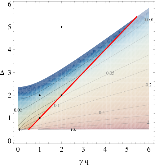
The zero temperature result of this plot can be understood analytically. If we look for a threshold unstable mode, with $\omega=0$, at zero temperature, then near the horizon we find the behaviour

$$\phi\sim(r-r_{+})^{(-3\pm\sqrt{3}\sqrt{3-q^{2}\gamma^{2}+2\Delta(\Delta-3)})/6}\,.$$

(14)

On general grounds one expects an instability to arise when the field oscillates infinitely many times before reaching the horizon [31]. From (14) we see that this requires

$$q^{2}\gamma^{2}\geq 3+2\Delta(\Delta-3)\,.$$

(15)

Therefore we expect an instability when the charge of the scalar field is sufficiently large as given by (15). If the charge is lower than the critical value there will never be an instability, as raising the temperature acts to stabilise the theory. The black line in figure 1, obtained numerically, is precisely the curve (15) separating stable backgrounds from backgrounds that become unstable below some temperature. This is a line of quantum critical points. It would be interesting to study in detail the dynamics close to these points.

The instability criterion (15) reduces to the inequality noted in [19] for the case of neutral scalar fields ($q=0$). There the result was obtained by comparing the mass squared of the field to the Breitenlohner-Freedman bound in the $AdS_{2}$ near horizon region. The full result (15) may be obtained by requiring the near horizon effective mass squared, including the coupling to the Maxwell field [32], to be below the $AdS_{2}$ Breitenlohner-Freedman bound.

The remaining noteworthy feature of figure 1, is that the critical temperature diverges as $\Delta\to{\textstyle{1\over 2}}$. This divergence is exhibited clearly in figure 2, which shows the critical temperature as a function of operator dimension along the BPS line $\Delta=\gamma q$. It is presumably related to the fact that $\Delta={\textstyle{1\over 2}}$ modes form singleton representations of the AdS₄ isometry group. These modes can be gauged to the boundary of AdS, which one thinks of as the UV of the field theory, and hence are not sensitive to the temperature, which only affects the IR physics. Thus the superconducting instability can never be stabilised by the temperature in this case. The field theory statement of this fact is that these modes are decoupled from all others and therefore do not acquire a thermal mass.

If we wish to find string theory realisations of holographic superconductivity, we need to find compactifications of string theory that have charged scalars with masses and charges that fall inside the shaded region to the left of the BPS line in figure 1.

A priori it is not obvious that there exist compactifications with charged scalars that lie in the left hand region of figure 1. An argument in favour of the generic presence of an instability comes from the conjectured ‘weak gravity’ bound [33]. Perhaps the sharpest of the statements in that paper was the requirement that extremal black holes should be able to decay in consistent theories of quantum gravity. In asymptotically Minkowski spacetime, a simple kinematic argument shows that this requirement implies that there must exist a charged particle in the theory that has mass and charge related by $m\leq\sqrt{2}gqM$, where $m,g,q$ and $M$ have the same meanings as they did in the previous subsections. The interest of this statement is that if $gq\ll 1$, then the charged particle is much lighter than would be predicted from standard effective field theory logic.

In asymptotically Anti-de Sitter spacetimes it is less straightforward to make kinematic arguments for a weak gravity bound, as particles may not scatter out to infinity. However, the criterion (15) for a classical instability was obtained from only the near horizon geometry of the extremal black hole. If the preferred decay mode of the black hole is through a minimally coupled scalar, as we have been assuming, then (15) is a natural candidate for the correct weak gravity bound. Namely, in any consistent asymptotically AdS theory of quantum gravity there should exist a charged particle with charge $q$ and energy $\Delta$ such that (15) is satisfied and extremal black holes can decay. We can note that (15) does not reduce to the Minkowski space bound when $\Delta\gg 1$. We are only considering large AdS black holes, smaller black holes can require a more stringent condition in order to decay.

A caveat to the above statement is the possibility of decaying through charged modes that are not minimally coupled scalars. Given a field with a specified spin and coupling to the Maxwell field, it is easy to rerun the above argument involving the near horizon Breitenlohner-Freedman bound and obtain an instability criterion analogous to (15). The weak gravity bound would only require the existence of one unstable mode, of any spin and coupling.

The instability we are describing is essentially Schwinger pair production. Although this is initially a quantum mechanical effect, once there is sufficient condensate accumulated it is described as a classical instability in terms of macroscopic fields. Whatever the microscopic mechanism for emission of charge from the black hole, it seems likely that the classical field instability considered here is the correct description once the number of quanta involved becomes large. Furthermore, numerical investigations in [19] suggested (but not conclusively) that at the endpoint of the extremal black hole instability, if the charge of the scalar field is nonzero, all of the charge is carried by the scalar field condensate. Therefore this instability leads to the complete decay of the extremal black hole, as required by the weak gravity conjecture.

An interesting exception to the statements in the previous paragraph might arise if the preferred decay mode of the black hole were to charged fermionic particles. In the absence of a pairing mechanism these will not develop macroscopic occupation numbers, but rather build up a fermi surface. This could lead to novel black holes with charged fermionic hair.

Whether or not one believes in the weak gravity bound, we shall now show that there indeed exist a large set of vacua in which extremal AdS-Reissner-Nordstrom black holes are unstable. Note that extremal AdS-Reissner-Nordstrom black holes are not supersymmetric and do not saturate the BPS bound.

The M theory bosonic action is (in the conventions of [34])

$$S=\frac{1}{2\kappa^{2}}\int d^{11}x\sqrt{-g}R-\frac{1}{\kappa^{2}}\int\left[G\wedge\star G+\frac{2}{3}C\wedge G\wedge G\right]\,,$$

(16)

with $G=dC$. We are interested in Freund-Rubin vacua with a background electromagnetic field in four dimensions. See for instance [35, 27]. The metric ansatz is

$$ds^{2}_{11}=L^{2}ds^{2}_{M_{4}}+4L^{2}\left[(a[d\psi+A]+\sigma)^{2}+ds^{2}_{M_{6}}\right]\,,$$

(17)

supported by the flux

$$G=\frac{3L^{3}}{2}\text{vol}_{M_{4}}-4L^{3}a\,\omega\wedge\star_{4}F\,,$$

(18)

where $\frac{1}{2}d\sigma=\omega$ is the Kähler form on $M_{6}$, which is taken to be a six real dimensional Kähler-Einstein manifold satisfying ${\rm Ric}_{M_{6}}=8\,g_{M_{6}}$, and $F=dA$. In (17) the coefficient $a$ is such that $\psi$ has range $2\pi$, and we have chosen the four dimensional gauge connection $A$ to be normalised so that excitations have integer charges.

One can check that (17) and (18) solve the eleven dimensional equations of motion if and only if the four dimensional metric $g^{(4)}$ and gauge field $A$ solve the four dimensional Einstein-Maxwell-AdS equations of motion. These come from the effective four dimensional Lagrangian density

$${\mathcal{L}}^{(4)}=\frac{1}{2\kappa^{2}_{4}}\left[R^{(4)}+\frac{6}{L^{2}}-4L^{2}a^{2}F_{\mu\nu}F^{\mu\nu}\right]\,,$$

(19)

where

$$\frac{1}{2\kappa^{2}_{4}}=\frac{(2L)^{7}\text{Vol}(M_{7})}{2\kappa^{2}}\,.$$

(20)

In this expression $M_{7}$ refers to the Sasaki-Einstein manifold⁶⁶ 6 We will only consider quasi regular Sasaki-Einstein manifolds, i.e. those for which the orbits of the Killing vector close. Hence the fibration is $U(1)$ rather than ${{\mathbb{R}}}$, and charges are quantised.

$$ds^{2}_{M_{7}}=(ad\psi+\sigma)^{2}+ds^{2}_{M_{6}}\,,$$

(21)

with unit radius, that is, $ds^{2}_{M_{7}}$ is such that the cone

$$ds_{M_{8}}^{2}=dr^{2}+r^{2}ds^{2}_{M_{7}}\,,$$

(22)

is Ricci flat, i.e. a Calabi-Yau fourfold. The construction of Sasaki-Einstein manifolds as $U(1)$ fibrations over Kähler-Einstein manifolds is reviewed with differing emphases in [36, 37, 38, 39]. The simplest example is $M_{7}=S^{7}$, the round 7-sphere, for which $M_{8}={{\mathbb{C}}}^{4}$, $M_{6}={\mathbb{CP}}^{3}$, $ds^{2}_{M_{6}}$ the Fubini-Study metric, and $a=1$. The $U(1)$ symmetry is the R-symmetry of the dual ${\mathcal{N}}=2$ field theory.

In checking that this ansatz indeed provides a consistent truncation to four dimensional Einstein-Maxwell with a negative cosmological constant, it is important to be precise about orientations. We are taking the Sasaki-Einstein metric to be orientated such that its volume form is

$$\text{vol}_{M_{7}}=+\frac{a}{6}d\psi\wedge\omega\wedge\omega\wedge\omega\,.$$

(23)

This implies, for instance, that

$$\star_{7}(\omega\wedge\omega)=+2(ad\psi+\sigma)\wedge\omega\,,$$

(24)

which is an equation one uses in confirming consistency.

Comparing the effective action (19) to our general expression in section 2 above we find that for these theories the ‘ratio of central charges’

$$\gamma=\sqrt{\frac{c}{96\sigma}}=\frac{1}{2a}\,.$$

(25)

The coefficient $\gamma$ is therefore determined by a single component of the Sasaki-Einstein metric, giving the (constant) radius of the canonical $U(1)$ fibration. This radius is determined topologically. Concretely:

$$\gamma=\frac{2k}{\gcd c_{1}(M_{6})}\,,$$

(26)

where $k$ is a positive integer and $\gcd c_{1}(M_{6})$ is the greatest integer by which the first Chern class $c_{1}(M_{6})$ can be divided such that it remains an integral (orbifold) cohomology class [39]. The freedom to choose $k$ corresponds to the freedom to quotient the circle by ${{\mathbb{Z}}}_{k}$. For example for $M_{7}=S^{7}/{{\mathbb{Z}}}_{k}$, since $\gcd c_{1}({{\mathbb{C}}}{\mathbb{P}}^{3})=4$, we get $\gamma=k/2$. There is a constraint on the values of $k$ that are compatible with supersymmetry. The Killing spinor has a $\psi$ dependence of the form $e^{i2a\psi}$ [36]. In order for the spinor to be well defined we must therefore have $4a\in{{\mathbb{Z}}}$. This constrains $k$ not to be too large, given $\gcd c_{1}(M_{6})$.

By comparison with section 2 we can also obtain the central charge

$$c=\frac{192\,L^{2}}{\kappa^{2}_{4}}=\frac{32\,\pi}{\sqrt{6}\text{Vol}(M_{7})^{1/2}}\,N^{3/2}\,.$$

(27)

In this expression we introduced the M2 brane charge $N\propto\int[*G+C\wedge G]$, which is a positive integer⁷⁷ 7 Specifically, $N=3(2L)^{6}\text{Vol}(M_{7})/(2\pi^{3}\kappa^{4})^{1/3}$. This normalisation can be obtained from the Dirac quantisation condition for M2 and M5 branes in M theory.. The dual 2+1 dimensional CFT, to be discussed below, will have an ultraviolet description as a gauge theory with an $SU(N)$ gauge group. Like the fiber radius $a$, the normalized volume ${\rm Vol}(M_{7})$ can be computed topologically [39]. Bishop’s theorem implies that $\text{Vol}(M_{7})\leq\text{Vol}(S^{7})=\pi^{4}/3$. Therefore the central charge (27) is always larger than the central charge of the maximally supersymmetric theory, $c_{{\mathcal{N}}=8}\approx 7.2\,N^{3/2}$.

A rich landscape of examples of Sasaki-Einstein manifolds is provided by links of Calabi-Yau hypersurface singularities. These are constructed as follows. Consider a weighted homogeneous polynomial $F(z)$ in ${{\mathbb{C}}}^{5}$. That is, satisfying

$$F(\lambda^{w_{1}}z_{1},\ldots,\lambda^{w_{5}}z_{5})=\lambda^{d}F(z_{1},\ldots,z_{5})\,,$$

(28)

where $w_{i}$ and $d$ are positive integers. An example is

$$F(z)=z_{1}^{2}+z_{2}^{5}+z_{3}^{6}+z_{4}^{7}+z_{5}^{8}=0\,,$$

(29)

which has ${\bf w}=(420,168,140,120,105)$ and $d=840$. The scaling action implies that the zero set $F(z)=0$ is a four complex dimensional cone in ${{\mathbb{C}}}^{5}$. By definition, if the hypersurface supports a conical Ricci flat Kähler metric as in (22), the base (link) of the cone is Sasaki-Einstein. The $U(1)$ acting as $\psi\to\psi+\Delta\psi$ on (21) acts as $z_{i}\to e^{iw_{i}\Delta\psi}z_{i}$ on the coordinates $z_{i}$. Thus the integrally quantised charge of the coordinate $z_{i}$ is precisely $w_{i}$. This will shortly enable us to obtain the integrally quantized charge $q$ of various 3-form modes from the weights $\{w_{i}\}$.

For these Sasaki-Einstein spaces the quantities $a$ and ${\rm Vol}(M_{7})$ introduced above, and therefore $\gamma$ and $c$, are known explicitly [40, 39]:

	$\displaystyle a$	$\displaystyle=$	$\displaystyle\frac{\sum_{i}w_{i}-d}{4}\,,$		(30)
	$\displaystyle\text{Vol}(M_{7})$	$\displaystyle=$	$\displaystyle\frac{\pi^{4}a^{4}d}{3\prod_{i}w_{i}}\,.$		(31)

Not every cone constructed in this manner supports a Ricci flat Kähler metric, and correspondingly not every link supports a Sasaki-Einstein metric. A necessary condition for existence is [41] $\min_{i}w_{i}\geq a>0$, with $a$ given by (30). The CFT interpretation of this bound is quite pretty [41]: it is the unitarity bound $\Delta\geq{\textstyle{1\over 2}}$ for chiral primaries corresponding to holomorphic functions on the cone. An example that violates this condition is the $A_{k}$ singularity $F(z)=z_{1}^{k+1}+z_{2}^{2}+z_{3}^{2}+z_{4}^{2}+z_{5}^{2}=0$ for $k>2$. A second necessary condition is the bound following from Bishop’s theorem [41] $\text{Vol}(M_{7})\leq\text{Vol}(S^{7})=\pi^{4}/3$, with $\text{Vol}(M_{7})$ given by (31).

A sufficient condition can be formulated [42] for the special case of Brieskorn-Pham cones, defined by Fermat type polynomials

$$F(z)=z_{1}^{m_{1}}+\cdots+z_{5}^{m_{5}}=0\,.$$

(32)

These are weighted homogeneous polynomials as in (28) above with

$$d=\text{lcm}(m_{i}|i=1..5)\,,\qquad w_{i}=\frac{d}{m_{i}}\,.$$

(33)

According to [42], if the coefficients satisfy the following two conditions, then the link is Sasaki-Einstein:

$$1<\sum_{i}\frac{1}{m_{i}}<1+\frac{4}{3}\min_{i,j}\left\{\frac{1}{m_{i}},\frac{1}{b_{i}b_{j}}\right\}\,.$$

(34)

In this expression

$$b_{j}=\gcd(m_{j},c_{j})\,,\qquad c_{j}=\text{lcm}(m_{i}|i\neq j)\,.$$

(35)

Furthermore, two such Sasaki-Einstein manifolds, corresponding to different exponents $\{m_{i}\}$ and $\{m_{i}^{\prime}\}$, are isomorphic if and only if the two sets of exponents are permutations of each other. These conditions are sufficient but not necessary for existence. A general necessary and sufficient condition is not known.

The example given in (29) satisfies the conditions (34). It yields a Sasaki-Einstein manifold with $a=28.25$ and ${\rm Vol}(M_{7})\approx 0.1396$, so $\gamma\approx 0.0177$ and $c\approx 110\,N^{3/2}$. The results reviewed in [44] imply that this manifold is homotopy equivalent (and therefore, by the generalized Poincaré conjecture, homeomorphic) but not diffeomorphic to the standard sphere $S^{7}$. That is, it can be continuously deformed into the round $S^{7}$ and there is a continuous but no smooth one to one map to the round $S^{7}$. Some further remarkable results about Sasaki-Einstein spaces constructed in this way may be found in [43, 44, 42].

Given the eleven dimensional background (17) and (18) of the previous subsection, we wish to know whether the AdS-Reissner-Nordstrom black hole (5) is unstable against charged excitations of the background. To answer this question systematically one should consider the general linearised perturbation of the eleven dimensional metric and 3-form about the background. While the spectrum of perturbations about neutral Freund-Rubin compactifications is a well-developed subject [34], the analysis is substantially complicated by the presence of a background four dimensional Maxwell field. Generically the various modes that appear diagonally in the spectrum about the neutral vacuum are not minimally coupled to the background Maxwell field and furthermore get mixed amongst each other. For example, one may get couplings such as $|\phi|^{2}F^{2}$, $\phi\,F^{\mu\nu}\partial_{\mu}v_{\nu}$ or $\phi\,\epsilon^{\mu\nu\rho\sigma}F_{\mu\nu}b_{\rho\sigma}$, where $v_{\mu}$ is some charged vector mode and $b_{\mu\nu}$ a charged 2-form mode. Moreover, such non-minimal couplings tend to qualitatively alter the stability analysis of section 2.2.

Rather then perform the full stability analysis we shall focus on particular 3-form modes which, remarkably, turn out to be only minimally coupled to the Maxwell field and decouple from all other perturbations at the linearised level, in any background satisfying the Einstein-Maxwell equations. We will then show that these modes are sufficient to establish instabilities in a large number of Sasaki-Einstein vacua at finite chemical potential. It should be borne in mind however that there may be more unstable modes than the ones we find. Therefore our results for critical temperatures should be taken as lower bounds only.

In order to describe these modes, it is useful to start with the eight dimensional Calabi-Yau cone (22). Consider a closed self-dual or anti-self-dual 4-form $\hat{Y}_{4}$ on the cone. That is

$$d\hat{Y}_{4}=0\,,\qquad\star_{8}\hat{Y}_{4}=s\hat{Y}_{4}\,,\qquad s=\pm 1\,.$$

(36)

These conditions imply that $\hat{Y}_{4}$ is harmonic. Assume furthermore that the 4-form is homogeneous with degree $n$ on the cone. That is

$${\mathcal{L}}_{r\partial_{r}}\hat{Y}_{4}=n\hat{Y}_{4}\,.$$

(37)

Here ${\mathcal{L}}$ denotes the Lie derivative. Then we can decompose the form as

$$\hat{Y}_{4}=r^{n}\left(\frac{dr}{r}\wedge Y_{3}+Y_{4}\right)\,,$$

(38)

with $Y_{3}$ and $Y_{4}$ being forms on the Sasaki-Einstein manifold $M_{7}$, and (36) implies

$$\star_{7}dY_{3}=snY_{3}\,,\qquad d\star_{7}Y_{3}=0\,.$$

(39)

Now consider the 3-form fluctuation

$$\delta C=\phi\,Y_{3}+\text{c.c.}\,,$$

(40)

where $\phi$ only depends on the four dimensional spacetime coordinates. The field $\phi$ will be a pseudoscalar because the 3-form field changes sign under space or time reflections [34]. From (39) one shows that in a neutral background with $A_{\mu}=0$ [34]:

$$\nabla^{\mu}\nabla_{\mu}\phi=m^{2}\phi\,,\qquad m^{2}=\frac{n(n+6s)}{4L^{2}}\,.$$

(41)

Moreover this mode does not source any other KK modes at linear order [34].

The question now is what happens when $A_{\mu}$ is nonzero. We claim the following:

If $\hat{Y}_{4}$ is a primitive and closed (4,0) or (3,1)-form on the Calabi-Yau fourfold, and $\{g_{\mu\nu},A_{\mu}\}$ solve the 4d Einstein-Maxwell equations, then the covariantization of the mode (40) linearly decouples from all other Kaluza-Klein modes and satisfies the covariantized equation of motion (41), with $s=+1$ for $(4,0)$-forms and $s=-1$ for $(3,1)$-forms.

Before sketching the proof, let us clarify the claim. Recall that a primitive middle dimensional form on a Kähler manifold is one that satisfies

$$\hat{\omega}\wedge\hat{Y}_{4}=0\quad\mbox{ or equivalently }\quad\hat{\omega}\cdot\hat{Y}_{4}=0\,,$$

(42)

where $\hat{\omega}$ is the Kähler form on the Calabi-Yau cone. Covariantization means replacing, in the coordinates of (21), $d\psi\to d\psi+A$ in (40), and $\nabla_{\mu}\to\nabla_{\mu}-iqA_{\mu}$ in (41), where we assumed the mode to have a definite charge $q$ under the canonical $U(1)$ symmetry of the cone:

$${\mathcal{L}}_{\partial_{\psi}}\hat{Y}_{4}=iq\hat{Y}_{4}\,.$$

(43)

This charge will be directly inherited by $Y_{3}$ and $Y_{4}$. Thus, explicitly, we take

$$\delta C=\phi\,Y_{3}^{A}+\text{c.c.}\,,$$

(44)

where $Y_{3}^{A}$ is obtained from $Y_{3}$ by replacing $d\psi$ by $d\psi+A$. In components

$$\delta C_{mnp}=\phi\,Y_{3\,mnp}\,,\qquad\delta C_{\mu mn}=\phi\,A_{\mu}Y_{3\,mn\psi}\,,$$

(45)

where $m,n,p$ are indices on $M_{7}$ and $\mu$ on $M_{4}$.

We will discuss the existence of modes $\hat{Y}_{4}$ satisfying all of the above conditions in the next subsection. For the moment we assume existence. To prove our claim, first note that the Kähler form on the cone may be decomposed as (see e.g. [39])

$$\hat{\omega}=r^{2}\left(\frac{dr}{r}\wedge\eta+\omega\right)\,,$$

(46)

where $d\eta=2\omega$, and $\omega$ is as before the Kähler form of $M_{6}$. In terms of the metric we wrote in (21) above, $\eta=ad\psi+\sigma$. The primitivity condition (42) is easily seen to imply

$$\omega\cdot Y_{3}=0\,,\qquad\omega\wedge Y_{3}+s\eta\wedge\star_{7}Y_{3}=0\,.$$

(47)

Here we also used (36). By plugging the mode (44) into the eleven dimensional equations of motion and using (47), we obtain⁸⁸ 8 We will not reproduce the straightforward but tedious computations here. We verified our results using the abstract tensor calculus package xAct [45]. the following three results:

• •

  Decoupling from metric fluctuations: The 3-form mode (44) does not source any linearised metric fluctuations provided that

  $$F\wedge F\left(\omega_{n}{}^{q}Y_{3\,mq\psi}+\omega_{m}{}^{q}Y_{3\,nq\psi}\right)=0\,.$$

  (48)

• •

  Decoupling from other 3-from modes: The 3-form mode (44) does not source any other linearised 3-form fluctuations provided that

  $$(s+1)\,\omega\wedge Y_{3}=0\,.$$

  (49)

• •

  Equation of motion for the pseudoscalar: If decoupling occurs, then the four dimensional pseudoscalar field satisfies

  $$\left(\nabla^{\mu}-iqA^{\mu}\right)\left(\nabla_{\mu}-iqA_{\mu}\right)\phi=m^{2}\phi\,,\qquad m^{2}=\frac{n(n+6s)}{4L^{2}}\,.$$

  (50)

  Solving this equation is sufficient to solve the full 11d linearised supergravity equations.

We now proceed to characterise forms for which (48) and (49) hold. In our electrically charged AdS-Reissner-Nordstrom background, $F\wedge F$ vanishes. Therefore the decoupling of metric fluctuations will be automatic. However, one might certainly wish to consider dyonic black holes also (for instance to study phenomena such as the Hall or Nernst effects [46, 47, 49]) for which this term does not vanish. Therefore in order to solve (48) we will require that $\omega_{n}{}^{q}Y_{3\,mq\psi}+\omega_{m}{}^{q}Y_{3\,nq\psi}=0$. There are (at least) four interesting cases in which this is true. These are if $\hat{Y}_{4}$ is a $(4,0)$, $(0,4)$, $(3,1)$ or $(1,3)$ form on the eight dimensional Calabi-Yau cone. Let us consider these cases one at a time.

If $\hat{Y}_{4}$ is a $(4,0)$ form, then $Y_{3\,mq\psi}$ is zero. This follows from the fact that $dr\wedge\eta$ is a $(1,1)$ form on the Calabi-Yau cone, see for instance (46). If $Y_{3}$ had a $d\psi$ component (i.e. an $\eta$ component), then $\hat{Y}_{4}$ in (38) would necessarily have an antiholomorphic component and could not be $(4,0)$. Hence $Y_{3\,mq\psi}$ is zero.

If $\hat{Y}_{4}$ is a $(3,1)$ form, then $Y_{3\,mq\psi}dx^{m}\wedge dx^{q}$ is a $(2,0)$ form. This again follows from the decomposition of $\hat{Y}_{4}$ in (38) and the fact that $dr\wedge\eta$ is a $(1,1)$ form. Given that both $m$ and $q$ are holomorphic indices it follows that $\omega_{n}{}^{q}Y_{3\,mq\psi}+\omega_{m}{}^{q}Y_{3\,nq\psi}=i(Y_{3\,mn\psi}+Y_{3\,nm\psi})=0$. The first of these equalities follows from the fact that $\omega_{m}{}^{q}$ is proportional to the complex structure while the second equality follows from antisymmetry of $Y_{3}$.

These arguments clearly go through identically when $\hat{Y}_{4}$ is $(0,4)$ or $(1,3)$. They do not work however when $\hat{Y}_{4}$ is a $(2,2)$ form. We can recall at this point that $(4,0)$ forms are always primitive (from (42)) and self-dual whereas primitive $(3,1)$ forms are anti-self-dual, in the canonical orientation with which we are working.

In order for (49) to vanish and other 3-form modes to decouple, we need that either $s=-1$ or that $\omega\wedge Y_{3}=0$. The first of these will hold if and only if $\hat{Y}_{4}$ is anti-self-dual whereas the second holds if $\hat{Y}_{4}$ is a $(4,0)$ form. This last statement follows from noting that the structure of the eight dimensional Kähler form (46) implies that $\frac{dr}{r}+i\eta$ is a holomorphic 1-form on the Calabi-Yau cone. Therefore in order for $\hat{Y}_{4}$ to be $(4,0)$ the decomposition (38) must take the form $\hat{Y}_{4}=r^{n}(\frac{dr}{r}\pm i\eta)\wedge Y_{3}$, with $Y_{3}$ a $(3,0)$ on the six dimensional Kähler-Einstein base of the Sasaki-Einstein manifold. However, if $Y_{3}$ is a $(3,0)$ form, then $\omega\wedge Y_{3}$ is zero.

This proves our claim. Summarising: The mode (44) decouples from all other perturbations if the closed 4-form $\hat{Y}_{4}$ is a $(4,0)$ or primitive $(3,1)$-form on the Calabi-Yau cone. It is described by a minimally coupled pseudoscalar in four dimensions with charge $q$ and mass squared

	$\displaystyle L^{2}m^{2}_{(4,0)}=\left(\frac{n}{2}+3\right)\frac{n}{2}\,,$		(51)
	$\displaystyle L^{2}m^{2}_{(3,1)}=\frac{n}{2}\left(\frac{n}{2}-3\right)\,.$		(52)

The same expressions hold for $(0,4)$ and $(1,3)$ forms, respectively. Using the relation $(Lm)^{2}=\Delta(\Delta-3)$, we can read off the possible conformal dimensions of the dual operators.

We will now establish the existence of modes in the classes described above, and confirm that in many examples they lead to instabilities and superconductivity at low temperatures.

All Calabi-Yau cones admit a canonical holomorphic $(4,0)$ form. This form is thus closed and self-dual. If we introduce holomorphic vielbeins $\theta^{a}$, $a$ runs from 1 to 4, such that the metric is written $ds^{2}_{M_{8}}=\theta^{a}\bar{\theta}^{a}$, then the form is given by

$$\hat{Y}_{4}=\hat{\Omega}_{4}\equiv\theta^{1}\wedge\theta^{2}\wedge\theta^{3}\wedge\theta^{4}\,.$$

(53)

It is immediate that this form has scaling dimension $n=4$ under the homothetic vector $r\partial_{r}$, as the metric has scaling dimension 2 and hence the $\theta^{a}$ have scaling dimension 1. Furthermore, we can easily obtain the charge $q=4a$ by noting that for this mode

$${\mathcal{L}}_{\partial_{\psi}}\hat{Y}_{4}=\partial_{\psi}\cdot d\hat{Y}_{4}+d(\partial_{\psi}\cdot\hat{Y}_{4})=d(\partial_{\psi}\cdot\hat{Y}_{4})=ai\,d(r^{4}Y_{3})=4ai\,\hat{Y}_{4}\,.$$

(54)

In the third and fourth equalities we used the fact noted previously that holomorphic 4-forms must take the form $\hat{Y}_{4}=r^{n}\left(\frac{dr}{r}+i\eta\right)\wedge Y_{3}$. In the last equality we also used the first expression in (47). It is clear that this argument will apply to any closed (4,0)-form with scaling dimension $n$, giving charge $q=na$. Such forms are readily obtained by multiplying $\hat{\Omega}_{4}$ by a homogeneous holomorphic function of degree $n-4$.

It follows from (25) that all of the Sasaki-Einstein vacua have a decoupled pseudoscalar mode with charge $\gamma q=2$ and, from (51), mass squared $m^{2}L^{2}=10$. This corresponds to an operator of dimension $\Delta=5$. Comparing with figure 1 or equation (15) we see that this mode never leads to an instability.

The recent results of [50] imply that this mode is part of a long vector⁹⁹ 9 And hence not part of a short hypermultiplet as was claimed in [51]. ${\rm OSp}(2|4)$ supermultiplet (the $E_{0}=4$, $y=0$ case in table 1 of [51]) which consistently decouples from all other Kaluza-Klein modes even at the nonlinear level. There are no other charged scalars in this multiplet.

Before moving on to consider a general class of $(3,1)$-forms, we can consider the special case of $M_{7}=S^{7}$ for which the Calabi-Yau cone is simply $M_{8}={{\mathbb{C}}}^{4}$. A $(3,1)$-form on ${{\mathbb{C}}}^{4}$ is given by, for instance,

$$\hat{Y}_{4}=d\bar{z}_{1}\wedge dz_{2}\wedge dz_{3}\wedge dz_{4}\,.$$

(55)

This is a closed, primitive, anti-self-dual $(3,1)$-form with $n=4$ and $\gamma q=1$, recalling that $a=1$ for the seven sphere. From (51) the four dimensional mass will be $m^{2}L^{2}=-2$, corresponding to $\Delta=2$ or $\Delta=1$. This is precisely the value of the mass studied in detail in [18, 19]. The two different dimensions of the dual operator correspond to theories that are related via a renormalisation group flow generated by a double trace deformation [52] . From figure 1 or equation (15) we see that this mode does condense at low temperatures. Therefore, the IR conformal fixed point of ${\mathcal{N}}=8$ $SU(N)$ Yang-Mills theory at large $N$ spontaneously breaks $U(1)_{R}$ and becomes a superconductor at low temperatures and nonzero chemical potential. Taking $\Delta=2$, we numerically find that the critical temperature is $T_{c}\approx 0.007\,\mu$. For $\Delta=1$, we get $T_{c}\approx 0.35\,\mu$. We recall this is a lower bound.¹⁰¹⁰ 10 There is another known instability for the case of $M_{7}=S^{7}$, the Gubser-Mitra instability [53, 54]. That instability corresponds to the charge becoming redistributed among the more than one $U(1)$ symmetry in the theory, and does not induce superconductivity, as all the operators involved are neutral. In our units $T_{\text{G-M}}=\mu/\pi\approx 0.32\mu$. Thus in the $\Delta=1$ case the superconducting instability kicks in before the Gubser-Mitra instability.

We now turn to our main source of examples, namely $(3,1)$-forms associated to complex structure moduli of the Calabi-Yau fourfold cone. Consider a metric deformation $\delta g_{ab}$, with $a$ and $b$ both holomorphic indices, preserving Ricci flatness. Then this is a Lichnerowicz zero mode and

$$\hat{Y}_{4}\equiv\delta g_{\bar{a}\bar{e}}\,{\hat{\Omega}_{4}^{\bar{e}}}{}_{bcd}\,d\bar{z}^{\bar{a}}\wedge dz^{b}\wedge dz^{c}\wedge dz^{d}\,,$$

(56)

is a harmonic (3,1) form [55]. In this equation a bar denotes an antiholomorphic index. It is easy to see that this form is furthermore primitive. We thus get an example of an anti-self-dual closed (3,1)-form, as considered above. Calabi-Yau metric deformations which preserve the cone structure (21)-(22), and are therefore moduli of the Sasaki-Einstein manifold, have the same scaling dimension as the metric and are neutral under the $U(1)$ isometry (otherwise they would not preserve the isometry and the metric would no longer be Sasaki-Einstein). Thus the associated $\hat{Y}_{4}$ has the same scaling dimension $n=4$ as $\hat{\Omega}_{4}$, and the same charge $\gamma q=2$. The mass formula (51) now implies $\Delta_{+}=2$, saturating the BPS bound.¹¹¹¹ 11 This mode is thus the lowest component of an OSp(2,4) hypermultiplet. Its scalar superpartner is the metric modulus fluctuation, which has $\gamma q=0$ and $\Delta_{+}=3$, as expected for a marginal deformation. Such modes always condense at low temperature, with (see figure 2 above)

$$T_{c}\approx 0.0416\,\frac{\mu}{\gamma}\,.$$

(57)

Therefore: The IR fixed point of ${\mathcal{N}}=2$ $SU(N)$ Yang-Mills theories at large $N$ with Sasaki-Einstein duals with at least one metric modulus become superconducting at temperatures below (57). As previously, this is a lower bound on $T_{c}$, there may be other unstable modes with higher critical temperatures.

Not all Sasaki-Einstein metrics have deformation moduli. For example the round sphere has none. However, many of the Brieskorn-Pham links introduced in section 3.2 have plenty of moduli, obtained as polynomial deformations of the same weight $d$ as the original polynomial (28). The number of such moduli equals the number of monomials of weight $d$ minus the number of coordinate transformations respecting the weights [56], that is

$$N_{\rm mod}=N_{\rm mon}(d)-\sum_{i}N_{\rm mon}(w_{i})\,,$$

(58)

where $N_{\rm mon}(w)$ stands for the number of monomials of weight $w$. For the example (29), $N_{\rm mod}=1$: There is precisely one deformation which cannot be reabsorbed in a weight preserving coordinate transformation, namely $\delta F(z)=\epsilon z_{3}^{3}z_{5}^{4}$. We shall look more systematically at the existence of moduli in the following section.

One could also consider deformations $\delta F=\epsilon F^{\prime}$ of the defining equation (28) with weight $d^{\prime}\neq d$. Such deformations do not preserve the cone structure, and so they are not moduli of the Sasaki-Einstein space. However if the fluctuation preserves the Ricci flatness of the cone metric to linear order, then (56) still gives a harmonic (3,1) form, and the corresponding pseudoscalar mode still satisfies all the required properties to be minimally coupled. To determine the charge of such a metric fluctuation it is useful to formally associate a charge $q_{\epsilon}=w_{\epsilon}=d-d^{\prime}$ to $\epsilon$. This way the polynomials $F$ and $\delta F$ would have the same charge $d$. The charge of the metric mode $\delta g_{ab}=\partial_{\epsilon}g_{ab}|_{\epsilon=0}$ is thus seen to be $-q_{\epsilon}=d^{\prime}-d$. The associated form mode (56) thus has charge $q$ and radial scaling dimension $n$ given by

$$\frac{n}{2}=\gamma q=2+\gamma(d^{\prime}-d)\,.$$

(59)

As an example, consider the deformation $\delta F=\epsilon z_{1}z_{2}^{2}$ of (29). This has $d^{\prime}=756$, and so, using $\gamma=\frac{2}{113}$, we get $\frac{n}{2}=\gamma q=\frac{58}{113}\approx 0.5132$. If this truly corresponded to a Calabi-Yau preserving deformation, it would give rise to a minimally coupled BPS pseudoscalar with this value of $\Delta=\gamma q$. This leads to $T_{c}=1.47318\frac{\mu}{\gamma}$, substantially higher than the cone-preserving modes (57). Determining in general when such modes are indeed Calabi-Yau preserving appears to be an interesting open mathematical problem [57]. We shall not address this problem here, but note that it could lead to higher values of $T_{c}$ than the ones we will discuss.

The gravity backgrounds that we have been describing are dual to ${\mathcal{N}}=2$ superconformal field theories. The supersymmetry and conformality follow directly from the global (super)symmetries of the gravitational solutions. In special cases there may be an enhancement of supersymmetry. For instance, when $M_{7}=S^{7}$ the theory has ${\mathcal{N}}=8$ supersymmetry and if $M_{7}$ is tri-Sasakian then the theory will have ${\mathcal{N}}=3$ supersymmetry.

More specifically, the dual field theory is that describing the worldvolume dynamics of $N$ M2 branes placed at the tip of a Calabi-Yau fourfold cone over the Sasaki-Einstein manifold $M_{7}$ [58]. Until recently, this relationship was not useful for obtaining an explicit description of the field theory degrees of freedom. On general grounds one might expect the M2 brane theories to arise as IR fixed points of multiple D2 brane gauge theories in a background obtained by dimensionally reducing the M theory geometry along the $U(1)$ isometry of the Sasaki-Einstein metric [59]. This reduction will break all the manifest supersymmetry of the background for generic (${\cal N}=2$) Sasaki-Einstein manifolds. This occurs because the Killing spinor is charged under the $U(1)$ isometry, as we recalled below (26).

A different brane construction for the case $M_{7}=S^{7}/{{\mathbb{Z}}}_{k}$ was presented in [60] (ABJM), following the renewed interest in multiple M2 brane theories initiated by [61, 62, 63]. The construction involves 2 NS5 branes, $N$ D3 branes and $k$ D5 branes. Upon T dualising and lifting to M theory one obtains $N$ multiple M2 branes probing a geometry that has local ${{\mathbb{C}}}^{4}/{{\mathbb{Z}}}_{k}$ singularities. The brane construction allowed [60] to identify the field theory as a specific superconformal $U(N)\times U(N)$ Chern-Simons theory at levels $k$ and $-k$.

The ABJM brane construction was generalised to a family of ${\mathcal{N}}=3$ field theories in [64]. These are dual to backgrounds in which $M_{7}$ is a tri-Sasakian manifold. The field theory dual for general ${\mathcal{N}}=2$ theories is not yet available, it appears that the most tractable subset of ${\mathcal{N}}=2$ theories are those in which the Calabi-Yau cone $M_{8}$ is toric (the Brieskorn-Pham cones we considered above are generally not toric). Combining the extensive intuition gained from toric ${\mathcal{N}}=1$ superconformal field theories in 3+1 dimensions and the ABJM construction, it has been proposed that the worldvolume theory of M2 branes probing toric Calabi-Yau cones is given by a quiver Chern-Simons theory [65, 66, 67, 68, 69, 70]. These have large gauge symmetries with associated gauge fields $A_{i}$ and complex scalar fields $\phi_{a}$ that are charged under the gauge symmetries. The supermultiplets are then completed with additional scalar and spinor fields. The action takes the form

	$\displaystyle S$	$\displaystyle=$	$\displaystyle\sum_{i}\frac{k_{i}}{4\pi}\int d^{3}x{\rm Tr}\left(A_{i}\wedge dA_{i}+\frac{2}{3}A_{i}\wedge A_{i}\wedge A_{i}+\text{superpartners}\right)$		(60)
		$\displaystyle+$	$\displaystyle\sum_{a}\int d^{3}x\left(\left|D\phi_{a}\right|^{2}-\left|\frac{\partial W}{\partial\phi_{a}}\right|^{2}+\text{superpartners}\right)\,.$

We are being somewhat schematic. The superpotential $W$ is a holomorphic function of the $\phi_{a}$. A thorough discussion of ${\mathcal{N}}=2$ Chern-Simons theories may be found in [71]. The point we would like to emphasise is that concrete field theory duals have been proposed for certain Sasaki-Einstein manifolds. One can therefore hope to identify the precise operator ${\mathcal{O}}$ which condenses at the superconducting instability.

The first mode we discussed in section 3.4 was obtained from the canonical holomorphic $(4,0)$-form on the Calabi-Yau cone. Although this mode did not lead to an instability, it is instructive to consider its dual field theory operator. The mode must be dual to a canonical operator which is present in all ${\mathcal{N}}=2$ theories. The most natural candidate is the superpotential itself: ${\mathcal{O}}=W$.¹²¹² 12 An analogous identification is implicitly made in the AdS₅/CFT₄ case with ${\mathcal{N}}=1$ supersymmetry in 3+1 dimensions in, for instance, [39]. As well as being holomorphic and canonical, this mode had charge $\gamma q=2$ which is also the R-charge of the superpotential. However, the mode has dimension $\Delta=5$, whereas the superpotential has classical dimension $\Delta=2$, as a consequence of being chiral. This identification would therefore imply that the dimension of the superpotential is renormalised in these 2+1 theories. This is consistent with the fact, mentioned in section 3.4, that this mode is part of a long multiplet [50], so its dimension is not protected.

The second set of modes we discussed were $(3,1)$-forms corresponding to complex moduli deformations of the Calabi-Yau cone. These must be canonically dual to deformations of the field theory that preserve supersymmetry and conformality. The most natural candidate dual operators are deformations of the superpotential, ${\mathcal{O}}=\delta W$. In this case our bulk mode was BPS, with charge and dimension $\Delta=\gamma q=2$, equal to those of bare superpotentials. These are relevant charged operators. This identification would indicate that whereas the overall superpotential is renormalised, deformations of the superpotential (if they exist) are not.

We also noted in section 3.4 that the $(3,1)$-form modes lie in a hypermultiplet which contained a scalar superpartner with $\gamma q=0$ and $\Delta=3$. This mode will be dual to a marginal deformation of the Lagrangian. If our previous identification with deformations of the superpotential is correct, these operators will be of the form ${\mathcal{O}}=\int d^{2}\theta\,\delta W+c.c.=\partial_{\phi^{a}}\partial_{\phi^{b}}\delta W\psi^{a}\psi^{b}+\cdots$, with $\psi^{a}$ fermionic superpartners of the $\phi^{a}$.

It is certainly of interest to flesh out these identifications further for cases in which the superpotential and its deformations are known explicitly. We will leave this for future work.

Given a (neutral) Freund-Rubin compactification from eleven to four dimensions, a different solution may be constructed by skew-whiffing [34]. One way to describe the skew-whiffed solution is to change the sign of the 3-form background with everything else held fixed. In terms of the ansatz (17) and (18), with $A=0$, this corresponds to letting $L\to-L$. In terms of brane constructions, this means that instead of $N$ M2 branes at the tip of a Calabi-Yau cone, one takes $N$ anti-M2 branes. This operation is not as innocuous as it might seem. With the exception of the case $M_{7}=S^{7}$, only one of the two solutions can be supersymmetric [34]. At the strict classical level, skew-whiffed solutions obtained from supersymmetric Freund-Rubin compactifications give examples of stable non-supersymmetric vacua [34]. Stability beyond the classical level is not known.

In the skew-whiffed backgrounds ($L\to-L$) it turns out that the construction of section 3.1 above does not give a consistent reduction to Einstein-Maxwell theory in general. This is because a relative sign changes between the kinetic and Chern-Simons term in the 3-form equations of motion. However, for a purely electric (or purely magnetic) background, such as the AdS-Reissner-Nordstrom black holes of interest to us, the Chern-Simons term vanishes and one does obtain a solution.

Perturbing the skew-whiffed charged background by our mode (44) one finds that both the decoupling conditions (48) and (49) and the equation of motion for the pseudoscalar (50) are changed by $s\to-s$. It follows from our previous arguments that only the modes obtained from closed $(4,0)$ and $(0,4)$ forms on the Calabi-Yau cone decouple in this case. Their mass squared is now given by

$$m^{2}_{(4,0)}=m^{2}_{(0,4)}=\frac{n(n-6)}{4L^{2}}\,.$$

(61)

We recalled above that all Calabi-Yau cones admit a closed $(4,0)$ form with $n=4$ and charge $\gamma q=2$. Therefore, all of the skew-whiffed backgrounds have a minimally coupled pseudoscalar with $m^{2}=-2$, corresponding to $\Delta=2$ or $\Delta=1$. We noted above (see figure 1) that these values of the charge and $\Delta$ lead to a superconducting instability at low temperatures. Therefore all theories dual to skew-whiffed Sasaki-Einstein compactifications of M theory are superconducting at low temperatures when placed at a finite chemical potential.

References

- [1] J. M. Maldacena, “The large N limit of superconformal field theories and supergravity,” Adv. Theor. Math. Phys. 2 (1998) 231 [Int. J. Theor. Phys. 38 (1999) 1113] [arXiv:hep-th/9711200].
- [2] R. Bousso and J. Polchinski, “Quantization of four-form fluxes and dynamical neutralization of the cosmological constant,” JHEP 0006, 006 (2000) [arXiv:hep-th/0004134].
- [3] S. Kachru, R. Kallosh, A. Linde and S. P. Trivedi, “De Sitter vacua in string theory,” Phys. Rev. D 68, 046005 (2003) [arXiv:hep-th/0301240].
- [4] L. Susskind, “The anthropic landscape of string theory,” arXiv:hep-th/0302219.
- [5] M. R. Douglas, “The statistics of string / M theory vacua,” JHEP 0305, 046 (2003) [arXiv:hep-th/0303194].
- [6] M. R. Douglas and S. Kachru, “Flux compactification,” Rev. Mod. Phys. 79, 733 (2007) [arXiv:hep-th/0610102].
- [7] F. Denef, “Les Houches Lectures on Constructing String Vacua,” arXiv:0803.1194 [hep-th].
- [8] M. Greiner and S. Fölling, “Condensed-matter physics: Optical lattices,” Nature 453, 736 (2008).
- [9] S. Sachdev, Quantum Phase Transitions, CUP, 1999.
- [10] S. Sachdev, “Quantum magnetism and criticality,” Nature Physics 4, 173 - 185 (2008) [arXiv:0711.3015 [cond-mat.str-el]].
- [11] O. Aharony, “The non-AdS/non-CFT correspondence, or three different paths to QCD,” arXiv:hep-th/0212193.
- [12] D. T. Son, “Toward an AdS/cold atoms correspondence: a geometric realization of the Schroedinger symmetry,” Phys. Rev. D 78, 046003 (2008) [arXiv:0804.3972 [hep-th]].
- [13] K. Balasubramanian and J. McGreevy, “Gravity duals for non-relativistic CFTs,” Phys. Rev. Lett. 101, 061601 (2008) [arXiv:0804.4053 [hep-th]].
- [14] S. Kachru, X. Liu and M. Mulligan, “Gravity Duals of Lifshitz-like Fixed Points,” Phys. Rev. D 78, 106005 (2008) [arXiv:0808.1725 [hep-th]].
- [15] E. Witten, “Anti-de Sitter space and holography,” Adv. Theor. Math. Phys. 2, 253 (1998) [arXiv:hep-th/9802150].
- [16] S. S. Gubser, I. R. Klebanov and A. M. Polyakov, “Gauge theory correlators from non-critical string theory,” Phys. Lett. B 428, 105 (1998) [arXiv:hep-th/9802109].
- [17] S. S. Gubser, “Breaking an Abelian gauge symmetry near a black hole horizon,” arXiv:0801.2977 [hep-th].
- [18] S. A. Hartnoll, C. P. Herzog and G. T. Horowitz, “Building a Holographic Superconductor,” Phys. Rev. Lett. 101, 031601 (2008) [arXiv:0803.3295 [hep-th]].
- [19] S. A. Hartnoll, C. P. Herzog and G. T. Horowitz, “Holographic Superconductors,” arXiv:0810.1563 [hep-th].
- [20] S. S. Gubser, “Colorful horizons with charge in anti-de Sitter space,” Phys. Rev. Lett. 101, 191601 (2008) [arXiv:0803.3483 [hep-th]].
- [21] S. S. Gubser and S. S. Pufu, “The gravity dual of a p-wave superconductor,” JHEP 0811, 033 (2008) [arXiv:0805.2960 [hep-th]].
- [22] M. M. Roberts and S. A. Hartnoll, “Pseudogap and time reversal breaking in a holographic superconductor,” JHEP 0808, 035 (2008) [arXiv:0805.3898 [hep-th]].
- [23] M. Ammon, J. Erdmenger, M. Kaminski and P. Kerner, “Superconductivity from gauge/gravity duality with flavor,” arXiv:0810.2316 [hep-th].
- [24] P. Basu, J. He, A. Mukherjee and H. H. Shieh, “Superconductivity from D3/D7: Holographic Pion Superfluid,” arXiv:0810.3970 [hep-th].
- [25] J. L. Cardy, “Anisotrpoic corrections to correlation functions in finite size systems,” Nucl. Phys. B 290, 355 (1987).
- [26] P. Kovtun and A. Ritz, “Black holes and universality classes of critical points,” Phys. Rev. Lett. 100, 171606 (2008) [arXiv:0801.2785 [hep-th]].
- [27] C. P. Herzog, P. Kovtun, S. Sachdev and D. T. Son, “Quantum critical transport, duality, and M-theory,” Phys. Rev. D 75, 085020 (2007) [arXiv:hep-th/0701036].
- [28] I. R. Klebanov and E. Witten, “AdS/CFT correspondence and symmetry breaking,” Nucl. Phys. B 556, 89 (1999) [arXiv:hep-th/9905104].
- [29] P. Kovtun and A. Ritz, “Universal conductivity and central charges,” arXiv:0806.0110 [hep-th].
- [30] L. J. Romans, “Supersymmetric, cold and lukewarm black holes in cosmological Einstein-Maxwell theory,” Nucl. Phys. B 383, 395 (1992) [arXiv:hep-th/9203018].
- [31] G. Gibbons and S. A. Hartnoll, “A gravitational instability in higher dimensions,” Phys. Rev. D 66, 064024 (2002) [arXiv:hep-th/0206202].
- [32] S. S. Gubser and A. Nellore, “Low-temperature behavior of the Abelian Higgs model in anti-de Sitter space,” arXiv:0810.4554 [hep-th].
- [33] N. Arkani-Hamed, L. Motl, A. Nicolis and C. Vafa, “The string landscape, black holes and gravity as the weakest force,” JHEP 0706, 060 (2007) [arXiv:hep-th/0601001].
- [34] M. J. Duff, B. E. W. Nilsson and C. N. Pope, “Kaluza-Klein Supergravity,” Phys. Rept. 130, 1 (1986).
- [35] J. P. Gauntlett and O. Varela, “Consistent Kaluza-Klein Reductions for General Supersymmetric AdS Solutions,” Phys. Rev. D 76, 126007 (2007) [arXiv:0707.2315 [hep-th]].
- [36] G. W. Gibbons, S. A. Hartnoll and C. N. Pope, “Bohm and Einstein-Sasaki metrics, black holes and cosmological event horizons,” Phys. Rev. D 67, 084024 (2003) [arXiv:hep-th/0208031].
- [37] C. P. Boyer and K. Galicki, “Sasakian Geometry, Hypersurface Singularities, and Einstein Metrics,” arXiv:math/0405256.
- [38] C. P. Boyer, “Sasakian Geometry: The Recent Work of Krzysztof Galicki,” arXiv:0806.0373 [math.DG].
- [39] D. Martelli, J. Sparks and S. T. Yau, “Sasaki-Einstein manifolds and volume minimisation,” arXiv:hep-th/0603021.
- [40] A. Bergman and C. P. Herzog, “The volume of some non-spherical horizons and the AdS/CFT correspondence,” JHEP 0201, 030 (2002) [arXiv:hep-th/0108020].
- [41] J. P. Gauntlett, D. Martelli, J. Sparks and S. T. Yau, “Obstructions to the existence of Sasaki-Einstein metrics,” Commun. Math. Phys. 273, 803 (2007) [arXiv:hep-th/0607080].
- [42] C. P. Boyer, K. Galicki and J. Kollar, “Einstein Metrics on Spheres,” Ann Math 162, 557 (2005) [arXiv:math/0309408].
- [43] C. P. Boyer and K. Galicki, “Einstein Metrics on Rational Homology Spheres,” arXiv:math/0311355.
- [44] C. P. Boyer, K. Galicki, J. Kollar and E. Thomas, “Einstein Metrics on Exotic Spheres in Dimensions 7, 11, and 15,” arXiv:math/0311293.
- [45] The xAct package is developed by José Martín-García and can be downloaded from http://metric.iem.csic.es/Martin-Garcia/xAct/index.html.
- [46] S. A. Hartnoll and P. Kovtun, “Hall conductivity from dyonic black holes,” Phys. Rev. D 76, 066001 (2007) [arXiv:0704.1160 [hep-th]].
- [47] S. A. Hartnoll, P. K. Kovtun, M. Muller and S. Sachdev, “Theory of the Nernst effect near quantum phase transitions in condensed matter, and in dyonic black holes,” Phys. Rev. B 76, 144502 (2007) [arXiv:0706.3215 [cond-mat.str-el]].
- [48] D. Adams, “The Hitchhiker’s Guide to the Galaxy”, Ballantine Books, 1979.
- [49] S. A. Hartnoll and C. P. Herzog, “Ohm’s Law at strong coupling: S duality and the cyclotron resonance,” Phys. Rev. D 76, 106012 (2007) [arXiv:0706.3228 [hep-th]].
- [50] J. P. Gauntlett, S. Kim, O. Varela and D. Waldram, “Consistent supersymmetric Kaluza–Klein truncations with massive modes,” arXiv:0901.0676 [hep-th].
- [51] A. Ceresole, P. Fre and H. Nicolai, “Multiplet Structure And Spectra Of N=2 Supersymmetric Compactifications,” Class. Quant. Grav. 2, 133 (1985).
- [52] E. Witten, “Multi-trace operators, boundary conditions, and AdS/CFT correspondence,” arXiv:hep-th/0112258.
- [53] S. S. Gubser and I. Mitra, “Instability of charged black holes in anti-de Sitter space,” arXiv:hep-th/0009126.
- [54] S. S. Gubser and I. Mitra, “The evolution of unstable black holes in anti-de Sitter space,” JHEP 0108, 018 (2001) [arXiv:hep-th/0011127].
- [55] P. Candelas and X. de la Ossa, “Moduli space of Calabi-Yau manifolds,” Nucl. Phys. B 355, 455 (1991).
- [56] C. P. Boyer and K. Galicki, “Sasakian Geometry”, Oxford Mathematical Monographs.
- [57] S.T. Yau, private communications.
- [58] I. R. Klebanov and E. Witten, “Superconformal field theory on threebranes at a Calabi-Yau singularity,” Nucl. Phys. B 536, 199 (1998) [arXiv:hep-th/9807080].
- [59] N. Itzhaki, J. M. Maldacena, J. Sonnenschein and S. Yankielowicz, “Supergravity and the large N limit of theories with sixteen Phys. Rev. D 58, 046004 (1998) [arXiv:hep-th/9802042].
- [60] O. Aharony, O. Bergman, D. L. Jafferis and J. Maldacena, “N=6 superconformal Chern-Simons-matter theories, M2-branes and their JHEP 0810, 091 (2008) [arXiv:0806.1218 [hep-th]].
- [61] J. Bagger and N. Lambert, “Modeling multiple M2’s,” Phys. Rev. D 75, 045020 (2007) [arXiv:hep-th/0611108].
- [62] A. Gustavsson, “Algebraic structures on parallel M2-branes,” arXiv:0709.1260 [hep-th].
- [63] J. Bagger and N. Lambert, “Gauge Symmetry and Supersymmetry of Multiple M2-Branes,” Phys. Rev. D 77, 065008 (2008) [arXiv:0711.0955 [hep-th]].
- [64] D. L. Jafferis and A. Tomasiello, “A simple class of N=3 gauge/gravity duals,” JHEP 0810, 101 (2008) [arXiv:0808.0864 [hep-th]].
- [65] D. Martelli and J. Sparks, “Notes on toric Sasaki-Einstein seven-manifolds and AdS4/CFT3,” JHEP 0811, 016 (2008) [arXiv:0808.0904 [hep-th]].
- [66] D. Martelli and J. Sparks, “Moduli spaces of Chern-Simons quiver gauge theories and AdS(4)/CFT(3),” arXiv:0808.0912 [hep-th].
- [67] A. Hanany and A. Zaffaroni, “Tilings, Chern-Simons Theories and M2 Branes,” JHEP 0810, 111 (2008) [arXiv:0808.1244 [hep-th]].
- [68] K. Ueda and M. Yamazaki, “Toric Calabi-Yau four-folds dual to Chern-Simons-matter theories,” JHEP 0812, 045 (2008) [arXiv:0808.3768 [hep-th]].
- [69] Y. Imamura and K. Kimura, “Quiver Chern-Simons theories and crystals,” JHEP 0810, 114 (2008) [arXiv:0808.4155 [hep-th]].
- [70] A. Hanany, D. Vegh and A. Zaffaroni, “Brane Tilings and M2 Branes,” arXiv:0809.1440 [hep-th].
- [71] D. Gaiotto and X. Yin, “Notes on superconformal Chern-Simons-matter theories,” JHEP 0708, 056 (2007) [arXiv:0704.3740 [hep-th]].
- [72] G. T. Horowitz and M. M. Roberts, “Holographic Superconductors with Various Condensates,” Phys. Rev. D 78, 126008 (2008) [arXiv:0810.1077 [hep-th]].
- [73] P. A. Lee, N. Nagaosa and X.-G. Wen, “Doping a Mott insulator: Physics of high temperature superconductivity”, Rev. Mod. Phys. 78, 17 (2006). [arXiv:cond-mat/0410445].