Studying Gaugino Mass Unification at the LHC
Baris Altunkaynak,(1) Phillip Grajek,(2) Michael Holmes,(1)
Gordon Kane,(2) and Brent D. Nelson(1)
(1) Department of Physics, Northeastern University, Boston, MA 02115
(2) Michigan Center for Theoretical Physics, Randall Lab.,
University of Michigan, Ann Arbor, MI 48109
We begin a systematic study of how gaugino mass unification can be probed at the CERN Large Hadron Collider (LHC) in a quasi-model independent manner. As a first step in that direction we focus our attention on the theoretically well-motivated mirage pattern of gaugino masses, a one-parameter family of models of which universal (high scale) gaugino masses are a limiting case. We improve on previous methods to define an analytic expression for the metric on signature space and use it to study one-parameter deviations from universality in the gaugino sector, randomizing over other soft supersymmetry-breaking parameters. We put forward three ensembles of observables targeted at the physics of the gaugino sector, allowing for a determination of this non-universality parameter without reconstructing individual mass eigenvalues or the soft supersymmetry-breaking gaugino masses themselves. In this controlled environment we find that approximately 80% of the supersymmetric parameter space would give rise to a model for which our method will detect non-universality in the gaugino mass sector at the 10% level with of integrated luminosity. We discuss strategies for improving the method and for adding more realism in dealing with the actual experimental circumstances of the LHC.
1 Introduction
As the Large Hadron Collider (LHC) era fast approaches, the theoretical community is increasingly focused on how the new discoveries made there will be interpreted. The first step, most obviously, is to establish the presence of physics beyond the Standard Model. This will be done using search strategies that are by now well-established, though many interesting “what-if” scenarios continue to be proposed and investigated [1]. We continue to believe that supersymmetry (SUSY) is the best-motivated extension to the Standard Model for physics at the LHC energy scale. Furthermore, if supersymmetry is indeed relevant at the electroweak scale there are many reasons to expect that its presence will be established early on in the LHC program [2]. Indeed, even some properties of the spectrum, such as the masses and spins of low-lying new states, may be crudely known even after relatively little integrated luminosity [3, 4, 5]. In this paper we begin a research program into what comes next: how to connect the multiple LHC observations to organizing principles in some (high-energy) effective Lagrangian of underlying physics.
This secondary problem can be further divided into two sub-problems. The first has come to be called the “inversion” problem. Briefly stated, the inversion problem is the recognition that even in very restrictive model frameworks it is quite likely that more than one set of model parameters will give predictions for LHC observations that are in good agreement with the experimental data [6]. Much recent work has focused on how to address this issue [7, 8, 9, 10, 11], and we will borrow much of the philosophy and many of the useful techniques from this recent literature. But our focus here is on what we might call the second sub-problem: how to turn the ensemble of distinct LHC signatures into a determination of certain broad properties of the underlying Lagrangian at low energies. Clearly the most direct attack on this second sub-problem is to perform a global fit to the parameters of a particular model [12, 13], modulo the degeneracy issue just described above. Not surprisingly, therefore, the work we will describe in this paper will make significant use of likelihood fits. But our ultimate goal is to fit to certain broad properties of the underlying physics itself – and not simply to a particular model of that physics.
We will refine this rather vague-sounding goal in a moment. But it is helpful to first consider an example of what we mean by the phrase “broad properties of the underlying physics.” Consider a high energy theorist interested in connecting the (supersymmetric) physics at the LHC to physics at an even higher energy scale, such as some underlying string theory. What sort of information would be of most use to him or her in this pursuit? Would it be a precise measurement of the gluino mass, or of the mass splitting in the top squark sector, or some other such measurement? Obtaining such information is (at least in principle) possible at the LHC, but far more valuable would be knowledge of the size of the supersymmetric -parameter or whether is very small. Such information is far more difficult to obtain at the LHC [14] but is more correlated with moduli stabilization and/or how the -parameter is generated in string models [15]. For example, this knowledge may tell us whether the -parameter is fundamental in the superpotential or generated via the Kähler potential as in the Giudice-Masiero mechanism [16]. This, in turn, is far more powerful in discriminating between potential string constructions than the gluino mass itself – no matter how accurately it is determined. We might refer to the genesis of the -parameter as a “broad property of the underlying physics.”
If all such key broad properties of the underlying physics were enumerated, it is our view that one of the most important such properties would be the question of gaugino mass universality. That is, the notion that at the energy scale at which supersymmetry breaking is transmitted to the observable sector, the gauginos of the minimal supersymmetric Standard Model (MSSM) all acquired soft masses of the same magnitude. This issue is intimately related to another, perhaps equally important issue: the wave-function of the lightest supersymmetric particle, typically the lightest neutral gaugino. Few properties of the superpartner spectrum have more far-reaching implications for low-energy phenomenology, the nature of supersymmetry breaking, and the structure of the underlying physics Lagrangian [17]. If the theorist could be told only one “result” from the LHC data the answer to the simple question “Is there evidence for gaugino mass universality?” might well be it. But these soft parameters are not themselves directly measurable at the LHC [18].11 1 Even a measurement of the physical gluino mass is not a direct measurement of the associated soft mass . Quantum corrections to the gluino bare mass can be sizable and their theoretical computation involves a large set of other MSSM soft parameters [19, 20] – which are also not directly measurable! One might consider performing a fit to some particular theory, such as minimal supergravity (mSUGRA), in which universal gaugino masses are assumed [21] – or perhaps to certain models with fixed, non-universal gaugino mass ratios [22, 23]. But we are not so much interested in whether mSUGRA – or any other particular theory for which gaugino mass universality is a feature – is a good fit to the data. Rather, we wish to know whether gaugino mass universality is a property of the underlying physics independent of all other properties of the model. From this example both the ambitiousness and the difficulty inherent in our task is clear.
We have therefore decided to begin our attack by considering a concrete parametrization of non-universalities in soft gaugino masses. Many such frameworks present themselves, but we will choose a parametrization that has the virtue of also having a strong theoretical motivation from string theory. In recent work by Choi and Nilles [24] soft supersymmetry-breaking gaugino mass patterns were explored in a variety of string-motivated contexts. In particular, the so-called “mirage pattern” of gaugino masses provides an interesting case study in gaugino mass non-universality. Yet as mentioned above, these soft supersymmetry breaking parameters are not themselves directly measurable. Linking the soft parameters to the underlying Lagrangian is important, but without the crucial step of linking the parameters to the data itself it will be impossible to reconstruct the underlying physics from the LHC observations.
The mirage paradigm gets its name from the fact that should the mirage pattern of gaugino masses be used as the low-energy boundary condition of the (one-loop) renormalization group equations then there will exist some high energy scale at which all three gaugino masses are identical. This unification has nothing to do with grand unification of gauge groups, however, and the gauge couplings will in general not unify at this particular energy scale – hence the name “mirage.” The set of all such low-energy boundary conditions that satisfy the mirage condition defines a one-parameter family of models. This parameter can be taken to be the mirage unification scale itself, or some other parameter, such as the ratio between various contributions to the gaugino soft masses. We note that the minimal supergravity paradigm of soft supersymmetry breaking is itself a member of this family of models since it is defined by the property that gaugino masses are universal at the scale . Indeed, in the parametrization we adopt from [24], the gaugino mass ratios at the electroweak scale take the form
| (1.1) |
where the case is precisely the unified mSUGRA limit. Note that when we speak of testing gaugino mass universality, therefore, we do not imagine a common gaugino soft mass at the low-energy scale. Instead, the “universality” paradigm implies the ratios
| (1.2) |
The goal of this work is to ask whether it is possible to determine that the parameter of (1.1) is different from zero – and if so, how.
The theoretical details behind the ratios of (1.1) will be the topic of Section 2 in this paper. These details are largely irrelevant for the analysis that follows in Sections 3 and 4, but may nevertheless be of interest to many readers. For those who are only interested in the methodology we will pursue and the results, this section can be omitted. At the end of Section 2 we will present two benchmark scenarios that arise from concrete realizations of the mirage pattern of gaugino masses in certain classes of string models. As this is a paper about the interface of theory and experiment at the LHC – and not about string phenomenology per se – we will leave the theoretical description of these models to the Appendix. In Section 3 we discuss how we will go about attempting to measure the value of the parameter in (1.1) and describe the process that led us to an ensemble of specific LHC observables targeted for precisely this purpose. In Section 4 this list of signatures is tested on a large collection of MSSM models, as well as on our two special benchmarks from Section 2. We will see that the signature lists constructed using the method of Section 3 do an excellent job of detecting the presence of non-universality in the gaugino soft masses over a very wide array of supersymmetric spectra hierarchies and mass ranges. Non-universality on the order of 30-50% should become apparent within the first 10 of analyzed data for most supersymmetric models consistent with current experimental constraints. Detecting non-universality at the 10% level would require an increase in data by roughly a factor of two. Nevertheless, depending on the details of the superpartner spectrum, some cases will require far more data to truly measure the presence of non-universality. Of course all of these statements must here be understood in the context of the very particular assumptions of this study. Some thoughts on how the process can be taken further in the direction of increased realism are discussed in the concluding section.
Before moving to the body of the paper, however, we would like to take a moment to emphasize a few broad features of the theoretical motivation behind the parametrization in (1.1). In the limit of very large values for the parameter the ratios among the gaugino masses approach those of the anomaly-mediated supersymmetry breaking (AMSB) paradigm [25, 26]. In fact, the mirage pattern is most naturally realized in scenarios in which a common contribution to all gaugino masses is balanced against an equally sizable contribution proportional to the beta-function coefficients of the three Standard Model gauge groups. Such an outcome arises in string-motivated contexts, such as KKLT-type moduli stabilization in D-brane models [27, 28] and Kähler stabilization in heterotic string models [29]. These string-derived manifestations can also be extended easily to include the presence of gauge mediation, in which the mirage pattern is maintained in the gaugino sector [30, 31]. Importantly, however, it can arise in non-stringy models, such as deflected anomaly mediation [32, 33]. We note that in none of these cases is the pure-AMSB limit likely to be obtained, so our focus here will be on small to moderate values of the parameter in (1.1).22 2 In any event, the phenomenology of the AMSB scenario is sufficiently distinct from the models we will consider that distinguishing between them should not be difficult [34]. We will further refine these observations in Section 2 before turning our attention to the measurement of the parameter at the LHC.
2 Theoretical Motivation and Background
In this section we wish to understand the origin of the mass ratios in (1.1) from first principles. We will treat the mirage mass pattern here in complete generality, without any reference to its possible origin from string-theoretic considerations. This short section concludes with two specific sets of soft parameters, both of which represent models with the mirage gaugino mass pattern (though the physics behind the rest of their soft supersymmetry breaking parameters are quite different). In the Appendix we will recast the discussion of this section in terms of the degrees of freedom present in low-energy effective Lagrangians from string model building. There we will also present the string theory origin of the two benchmark models that appear in Table 1 at the end of this section.
Let us begin by imagining a situation in which there are two contributions to the soft supersymmetry breaking gaugino masses. We assume that these contributions arise at some effective high-energy scale at which supersymmetry breaking is transmitted from some hidden sector to the observable sector. Let us refer to this scale as simply the ultraviolet scale . It is traditional in phenomenological treatments to take this scale to be the GUT scale at which gauge couplings unify, but in string constructions one might choose a different (possibly higher scale) at which the supergravity approximation for the effective Lagrangian becomes valid. We will further assume that one contribution to gaugino masses is universal in nature while the other contribution is proportional to the beta-function coefficient of the Standard Model gauge group. More specifically, consider the universal piece to be given by
| (2.3) |
where labels the Standard Model gauge group factors and represents some mass scale in the theory. The second piece is the so-called anomaly mediated piece, which arises from loop diagrams involving the auxiliary scalar field of supergravity [35, 36]. It will take the form
| (2.4) |
where the are the beta-function coefficients for the Standard Model gauge groups. In our conventions these are given by
| (2.5) |
where , are the quadratic Casimir operators for the gauge group , respectively, in the adjoint representation and in the representation of the matter fields charged under that group.33 3 The convention chosen in (2.5) is opposite of the one chosen in [37]. For the MSSM these are
| (2.6) |
Note that if we take then we have
| (2.7) |
The mass scale is common to all three gauge groups; the subscript is meant to indicate that the contribution in (2.4) is related to the gravitino mass. The full gaugino mass at the high energy boundary condition scale is therefore
| (2.8) |
Now imagine evolving the boundary conditions in (2.8) to some low-energy scale via the (one-loop) renormalization group equations (RGEs). For the anomaly-generated piece of (2.4) we need only replace the gauge coupling with the value at the appropriate scale
| (2.9) |
while for the universal piece we can use the fact that is a constant for the one-loop RGEs. After some manipulation this yields
| (2.10) |
Combining (2.10) and (2.9) gives the low scale expression
| (2.11) |
For gaugino masses to be unified at the low scale then the quantity in the square brackets in (2.11) must be engineered to vanish. This can be achieved with a judicious choice of the values and for a particular high-energy input scale . Put differently, for a given (such as the GUT scale) and a given overall scale , there is a one-parameter family of models defined by the choice .
It is possible, however, to find a more convenient parametrization of the family of gaugino mass patterns defined by (2.11). Consider defining the parameter by
| (2.12) |
so that (2.11) becomes
| (2.13) |
and the requirement of universality at the scale now implies . Normalizing the three gaugino masses by and evaluating the gauge couplings at a scale we obtain the mirage ratios
| (2.14) |
for , in good agreement with the expression in (1.1).
Let us generalize the parametrization in (2.12) once more. Instead of defining the parameter in terms of the starting and stoping points in the RG evolution of the gaugino mass parameters, we will fix them in terms of mass scales in the theory itself. Thus we follow the convention of Choi et al. [38] and define
| (2.15) |
where is the reduced Planck mass . Our parametrization is now divorced from the boundary condition scales of the RG flow and can be fixed in advance. The choice of mass parameters in the logarithm of (2.15) may seem arbitrary – and at this point it is indeed completely arbitrary – but they have been chosen so as to make better contact with string constructions, such as those which we present in the Appendix. Inserting (2.15) into (2.11) yields
| (2.16) | |||||
Comparing this expression with (2.10) it is clear if gauge couplings unify at a scale , then we should expect the soft supersymmetry breaking gaugino masses to unify at an effective scale given by
| (2.17) |
We see that our parametrization in terms of is indeed equivalent to a parametrization in terms of the effective unification scale, as suggested in the introduction.
The value of as defined in (2.12) or (2.15) can be crudely thought of as the ratio of the anomaly contribution to the universal contribution to gaugino masses. Indeed, the limit is the limit of the minimal supergravity paradigm, while is the AMSB limit. But as (2.8) makes clear, these two contributions will be of comparable size only if is at least an order of magnitude larger than . We could therefore have chosen a parametrization based on the ratio , with interesting values being in the range . But such a parametrization spoils the simple relation with the mirage unification scale (2.17). Furthermore, the introduction of the factor in (2.15) provides the needed large factor, taking a value of for TeV. To obtain the mirage pattern it is therefore necessary for the underlying theory to generate some large number . Specific examples of how this is achieved in explicit string-based models are given in the Appendix to this paper.
| Parameter | Point A | Point B | Parameter | Point A | Point B | |
| 0.3 | 1.0 | |||||
| 1.5 TeV | 16.3 TeV | |||||
| 198.7 | 851.6 | |||||
| 172.1 | 553.3 | , | ||||
| 154.6 | 339.1 | |||||
| 193.0 | 1309 | |||||
| 205.3 | 1084 | |||||
| 188.4 | 1248 | |||||
In Table 1 we have collected the necessary soft supersymmetry-breaking parameters to completely specify two benchmark points for further analysis in what follows. The details behind these two models are described in the Appendix. Here we will simply indicate that point A represents a heterotic string model with Kähler stabilization of the dilaton which was studied in detail in [37]. This particular example has a value of . Point B is an example from a class of Type IIB string compactifications with fluxes which was studied in [38]. This second example has a value . Both are examples of the mirage pattern of gaugino masses, having mirage unification scales of and , respectively. Note that these soft supersymmetry breaking terms are taken to be specified at the GUT energy scale of and must be evolved to electroweak scale energies through the renormalization group equations.
3 Determining : Methodology
3.1 Setting Up the Problem
As mentioned in the introduction, the ultimate goal of this avenue of study is to determine whether or not soft supersymmetry breaking gaugino masses obey some sort of universality condition independent of all other facts about the supersymmetric model. Such a goal cannot be met in a single paper so we have begun by asking a simpler question: assuming the world is defined by the MSSM with gaugino masses obeying the relation (1.1), how well can we determine the value of the parameter . At the very least we would like to be able to establish that with a relatively small amount of integrated luminosity. The first step in such an incremental approach is to demonstrate that some set of “targeted observables” [12] (we will call them “signatures” in what follows) is sensitive to small changes in the value of the parameter in a world where all other parameters which define the SUSY model are kept fixed. In subsequent work we intend to relax this strong constraint and treat the issue of gaugino mass universality more generally. Despite the lack of realism we feel this is a logical point of departure – very much in the spirit of the “slopes” of the Snowmass Points and Slopes [39] and other such benchmark studies. Thus, where the Snowmass benchmarks talk of slopes, we will here speak of “model lines” in which all parameters are kept fixed but the value of is varied in a controlled manner.
To construct a model line we must specify the supersymmetric model in all aspects other than the gaugino sector. The MSSM is completely specified by 105 distinct parameters, but only a small subset are in any way relevant for the determination of LHC collider observables [14]. We will therefore choose a simplified set of 17 parameters as in the two benchmark models of Table 1
| (3.18) |
The parameters in (3.18) are understood to be taken at the electroweak scale (specifically ) so no renormalization group evolution is required. The gluino soft mass will set the overall scale for the gaugino mass sector. The other two gaugino masses and are then determined relative to via (2.14). A model line will take the inputs of (3.18) and then construct a family of theories by varying the parameter from (the mSUGRA limit) to some non-zero value in even increments.
For each point along the model line we pass the model parameters to PYTHIA 6.4 [40] for spectrum calculation and event generation. Events are then sent to the PGS4 [41] package to simulate the detector response. Additional details of the analysis will be presented in later sections. The end result of our procedure is a set of observable quantities that have been designed and (at least crudely) optimized so as to be effective at separating from other points along the model line in the least amount of integrated luminosity possible. In Section 3.2 we describe the manner in which we perform this separation between models. The signature lists, and the analysis behind their construction, is presented in Section 3.3. In Section 4 we will demonstrate the effectiveness of these signature lists on a large sample of randomly generated model lines and provide some deeper insight on why the whole procedure works by examining our benchmarks in greater detail.
3.2 Distinguishability
The technique we will employ to distinguish between candidate theories using LHC observables was suggested in [12] and subsequently refined in [6]. The basic premise is to construct a variable similar to a traditional chi-square statistic
| (3.19) |
where is some observable quantity (or signature). The index labels these signatures, with being the total number of signatures considered. The labels and indicate two distinct theories which give rise to the signature sets and , respectively. Finally, the error term is an appropriately-constructed measure of the uncertainty of the term in the numerator, i.e. the difference between the signatures. In this work we will always define a signature as an observation interpreted as a count (or number) and denote it with capital . One example is the number of same-sign, same-flavor lepton pairs in a certain amount of integrated luminosity. Another example is taking the invariant mass of all such pairs and forming a histogram of the results, then integrating from some minimum value to some maximum value to obtain a number. In principle there can be an infinite number of signatures defined in this manner. In practice experimentalists will consider a finite number and many such signatures are redundant.
We can identify any signature with an effective cross section via the relation
| (3.20) |
where is the integrated luminosity. We refer to this as an effective cross-section as it is defined by the counting signature which contains in its definition such things as the geometric cuts that are performed on the data, the detector efficiencies, and so forth. Furthermore these effective cross sections, whether inferred from actual data or simulated data, are subject to statistical fluctuations. As we increase the integrated luminosity we expect that this effective cross section (as inferred from the data) converges to an “exact” cross section given by
| (3.21) |
These exact cross sections are (at least in principle) calculable predictions of a particular theory, making them the more natural quantities to use when trying to distinguish between theories. The transformation in (3.20) allows for a comparison of two signatures with differing amounts of integrated luminosity. This will prove useful in cases where the experimental data is presented after a limited amount of integrated luminosity , but the simulation being compared to the data involves a much higher integrated luminosity . Using these notions we can re-express our chi-square variable in terms of the cross sections
| (3.22) |
We will assume that the errors associated with the signatures are purely statistical in nature and that the integrated luminosities and are precisely known, so that
| (3.23) |
and therefore is given by
| (3.24) |
where each cross section includes the (common) Standard Model background, i.e. .
The variable forms a measure of the distance between any two theories in the space of signatures defined by the . We can use this metric on signature space to answer the following question: how far apart should two sets of signatures and be before we conclude that theories and are truly distinct? The original criterion used in [6] was as follows. Imagine taking any supersymmetric theory and performing a collider simulation. Now choose a new random number seed and repeat the simulation. Due to random fluctuations we expect that even the same set of input parameters, after simulation and event reconstruction, will produce a slightly different set of signatures. That is, we expect since it involves the effective cross-sections as extracted from the simulated data. Now repeat the simulation a large number of times, each with a different random number seed. Use (3.24) to compute the distance of each new simulation with the original simulation in signature space. The set of all values so constructed will form a distribution. Find the value of in this distribution which represents the 95th percentile of the distribution. This might be taken as a measure of the uncertainty in “distance” measurements associated with statistical fluctuations.
This procedure for defining distinguishability is unwieldy in a number of respects. Determining the threshold for separating models by is computationally intensive as it requires many repeated simulations of the same model (as well as the Standard Model background). More importantly, the “brute force” determination of is particular to model as well as the list of signatures used in (3.24). Each change in either the model parameters or the signature mix demands a new determination of the threshold for distinguishability. We will therefore propose a new criterion that has the benefit of being analytically calculable with a form that is universal to any pair of models and any set of signatures.
To do that let us reconsider the quantum fluctuations. At a finite integrated luminosity we can describe the outcome of a counting experiment as a Poisson distribution approximated by a normal distribution (this is a good approximation for approximately 10 counts or more), which can be expressed as
| (3.25) |
Here is a standard random variable, i.e. a random variable having a normal distribution centered at 0 with a standard deviation of 1. Note that by introducing statistical fluctuations via the variable we can replace in (3.25) with the exact cross section. Equation (3.25) then merely states the well known fact that the distribution in measured values should form a normal distribution about the value . To combine two such distributions and we may write
| (3.26) | |||||
where is a new standard random variable and is the total cross-section. For example, might be the contribution to a particular final state arising from Standard Model processes while might be the contribution arising from production of supersymmetric particles.
With the above in mind we can re-visit the definition (3.24) and obtain an analytic approximation for the distribution in values by using random variables to represent the signatures. The measured cross sections can be related to the exact cross sections via
| (3.27) |
with a similar expression for the model . Substituting (3.27) into (3.24) gives
| (3.28) | |||||
where we have combined and into the random variables and and have assumed that and are sufficiently large to be able to neglect the term proportional to . In this limit we immediately see that is itself a random variable with a probability distribution for the quantity given by
| (3.29) |
where is the non-central chi-squared distribution for degrees of freedom.44 4 If we had chosen to define the separation variable (3.19) without the factor of we would have found that the distribution of values was exactly given by the non-central chi-square distribution. The two are related by a simple change of variables. The non-centrality parameter is given by
| (3.30) |
and now the represent exact cross sections. This is actually the result we expect since the original in (3.24) is essentially a chi-square like function. Note that since the in the distribution of (3.28) are exact, we have the anticipated result that fluctuations of the quantity should be given by the central chi-square distribution . We note, however, that the derivation of (3.28) implicitly assumed that the signatures which we consider are uncorrelated – or more precisely that the fluctuations in these signatures are uncorrelated. We will have more to say about signature correlations in Section 3.3 below. We now have a measure of separation in signature space that is related to well known functions in probability theory.55 5 In fact, the non-central chi-square distribution is related to the regularized confluent geometric functions .

Armed with this technology, let us return to the issue of distinguishing a model from itself. From (3.28), (3.29) and (3.30) it is apparent that all the physics behind the distribution of possible values is contained in the values of and . In particular the distribution of possible values (a central chi-square distribution) should depend only on the number of signatures considered – not on the model point nor on the nature of those signatures. When comparing a model with itself we can therefore dispense with the subscript and write . We plot the probability distribution of (3.29) for and various values of in the top panel of Figure 1. We have also plotted the cumulative distribution function for the same values in the lower panel of Figure 1. To rule out the null hypothesis (i.e. the hypothesis that models and are in fact the same model) to a level of confidence requires demanding that is larger than the -th percentile value for the distribution (3.29) for the appropriate value. For example, if we use the criterion from [6] and require then . We have indicated this value for the cumulative distribution function by the horizontal dashed line in Figure 1. In general we will denote this particular value of for each value of by the symbol . It can be found via the cumulative distribution function as in Figure 1, or by numerically solving the equation
| (3.31) |
where is Euler’s gamma function and is the incomplete gamma function. A summary of these values for smaller values is given in Table 2. If we measure our signatures, extract the cross-sections, form and the number is greater than then we can say that the null hypothesis can be ruled out at a level of confidence given by %. The value of this critical is a universal number determined only by our choice of value and the number of signatures that we choose to consider.
| Confidence Level | ||||
|---|---|---|---|---|
| n | 0.95 | 0.975 | 0.99 | 0.999 |
| 1 | 3.84 | 5.02 | 6.64 | 10.83 |
| 2 | 3.00 | 3.69 | 4.61 | 6.91 |
| 3 | 2.61 | 3.12 | 3.78 | 5.42 |
| 4 | 2.37 | 2.79 | 3.32 | 4.62 |
| 5 | 2.21 | 2.57 | 3.02 | 4.10 |
| 6 | 2.10 | 2.41 | 2.80 | 3.74 |
| 7 | 2.01 | 2.29 | 2.64 | 3.48 |
| 8 | 1.94 | 2.19 | 2.51 | 3.27 |
| 9 | 1.88 | 2.11 | 2.41 | 3.10 |
| 10 | 1.83 | 2.05 | 2.32 | 2.96 |
If, however, our measurement gives then we cannot say the two models are distinct, at least not at the confidence level . But they may still be separate models and we were simply unfortunate, with statistical fluctuations producing a small value of . If we accumulate more data and measure again, we may find a different result. To quantify the probability that two different models and will give a particular value of requires the use of the non-central chi-square distribution in (3.29). The degree of non-centrality is given by the quantity in (3.30). Clearly, the more distinct the predictions and are from one another, the larger this number will be. In Figure 2 we plot the distribution for for signatures and several values of . As expected, the larger this parameter is, the more likely we are to find large values of .

Let us assume for the moment that “model ” is the experimental data, which corresponds to an integrated luminosity of . Our “model ” can then be a simulation with integrated luminosity . We might imagine that can be arbitrarily large, limited only by computational resources.66 6 Among other benefits of a large value for would be the reduction in uncertainties arising from the simulation side of the comparison, i.e. assuming that the simulation perfectly captures both the physics and the detector response, the remaining uncertainty would be that associated with the experimental observation associated with . We can then rewrite (3.30) as
| (3.32) |
From this expression it is clear that we can expect the value of this parameter to increase as experimental data is collected. The larger the value of the less likely it becomes to find a particularly small value of . This confirms out basic intuition that given any observable (or set of observables) for which the two models predict different values then with sufficient integrated luminosity it should always be possible to distinguish the models to arbitrary degree of confidence.
For any given value of , the probability that a measurement of will fluctuate to a value so small that it is not possible to separate two distinct models (to confidence level ) is simply the fraction of the probability distribution in (3.29) that lies to the left of the value . If we wish to be at least 95% certain that our measurements will correctly recognize that two different models are indeed distinct we must require
| (3.33) |
Since the value of the integral in (3.33) decreases monotonically as increases the value of this parameter which makes (3.33) an equality is the minimum non-centrality value such that the two models can be distinguished.
| Confidence Level | ||||
|---|---|---|---|---|
| n | 0.95 | 0.975 | 0.99 | 0.999 |
| 1 | 12.99 | 17.65 | 24.03 | 40.71 |
| 2 | 15.44 | 20.55 | 27.41 | 44.99 |
| 3 | 17.17 | 22.60 | 29.83 | 48.10 |
| 4 | 18.57 | 24.27 | 31.79 | 50.66 |
| 5 | 19.78 | 25.71 | 33.50 | 52.88 |
| 6 | 20.86 | 26.99 | 35.02 | 54.88 |
| 7 | 21.84 | 28.16 | 36.41 | 56.71 |
| 8 | 22.74 | 29.25 | 37.69 | 58.40 |
| 9 | 23.59 | 30.26 | 38.89 | 59.99 |
| 10 | 24.39 | 31.21 | 40.02 | 61.48 |
In other words for two distinct models and , any combination of experimental signatures such that will be effective in demonstrating that the two models are indeed different 95% of the time, with a confidence level of 95%. We have successfully reduced the problem to an exercise in pure mathematics, as these values can be calculated analytically without regard to the physics involved. A collection of values for small values of are given in Table 3. Note that as we increase the necessary value increases, reflecting the fact that as more observations are made we should expect that it will become increasingly likely that at least one will show a large deviation. Indeed, the quantity can be thought of as a measure of the overall distance from in the -dimensional signature space in units of the variances. As an example, again consider the case where . For this value of the corresponding value can be found from Table 2, while we can find from Table 3. We plot the distributions (3.29) for and simultaneously in Figure 3. By construction, the area of the non-central distribution to the left of the indicated value of will be precisely 5% of the total area.

Having reached the end of our somewhat lengthy digression on probability theory we now return to the physics issue at hand. The requirement that can be translated into a condition on the signature set and/or luminosity via the definition in (3.32). Let us make one final notational definition
| (3.34) |
where has the units of a cross section. Our condition for 95% certainty that we will be able to separate two truly distinct models at the 95% confidence level becomes
| (3.35) |
Given two models and and a selection of signatures both and are completely determined. Therefore the minimum amount of integrated luminosity needed to separate the models experimentally will be given by
| (3.36) |
We will be using (3.36) repeatedly throughout the rest of this paper. A well-chosen set of signatures will be the set that makes the resulting value of determined from (3.36) as small as it can possibly be.
3.3 Specific Signature Choice
Following the discussion in Section 3.2 we are in a position to define the goal behind our signature selection more precisely. We wish to select a set of signatures such that the quantity as defined in (3.36), for a given value of , is as small as it can possibly be over the widest possible array of model pairs and . We must also do our best to ensure that the signatures we choose to consider are reasonably uncorrelated with one another so that the statistical treatment of the preceding section is applicable. We will address the latter issue below, but let us first turn our attention to the matter of optimizing the signature list.
We took as our starting point an extremely large initial set of possible signatures. These included all the counting signatures and most of the kinematic distributions used in [6], all of the signatures of [42], several “classic” observables common in the literature [43] and several more which we constructed ourselves. Removing redundant instances of the same signature this yielded 46 independent counting signatures and 82 kinematic distributions represented by histograms, for 128 signatures in total. We might naively think that the best strategy is to include all of these signatures in the analysis (neglecting for now the issue of possible correlations among them). In fact, if the goal is statistically separating two models, the optimal strategy is generally to choose a rather small subset of the total signatures. Let us understand why that is the case. To do so we need a quantitative way of establish an absolute measure of the “power” of any given signature to separate two models and . This can be provided by considering the condition in (3.36). For any signature we can define an individual by
| (3.37) |
where, for example, . This quantity is exactly the integrated luminosity required to separate models and , to confidence level , by using the single observable . For a list of signatures it is possible to construct such values and order them from smallest value (most powerful) to largest value (least powerful). If we take any subset of these, then the requisite that results from considering all simultaneously is given by
| (3.38) |
Referring back to Table 3 we see that the ratio grows with . This indicates that as we add signatures with ever diminishing values we will eventually encounter a point of negative returns, where the resulting overall starts to grow again.
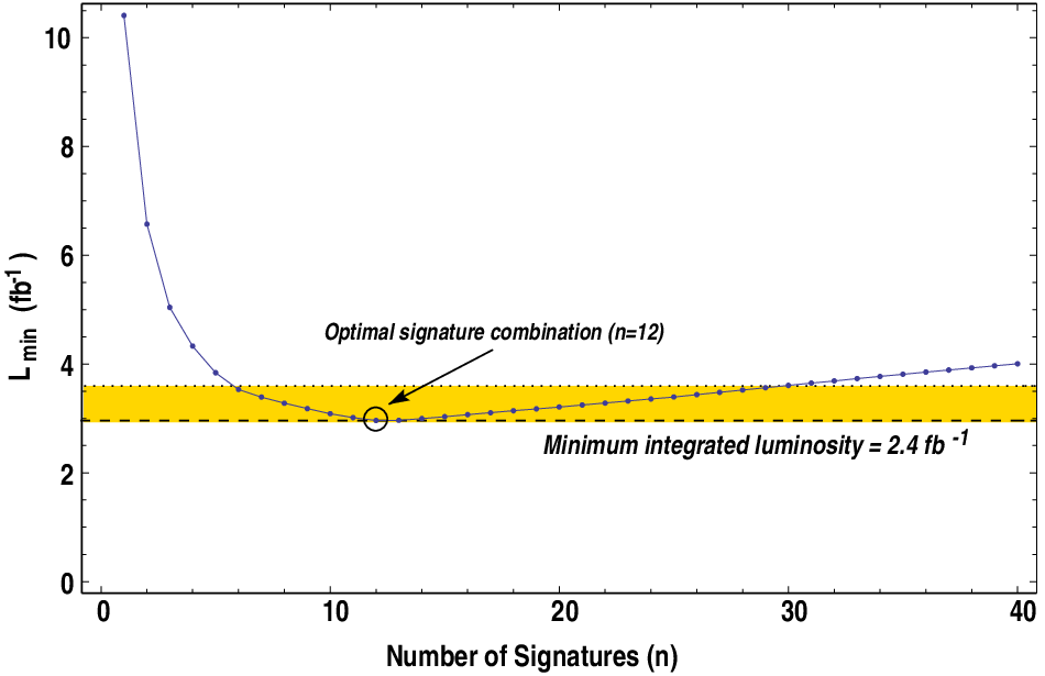
As more signatures are added, the threshold for adding the next signature in the list gets steadily stronger. For a particular pair of models, and , it is always possible to find the optimal list of signatures from among a given grand set by ordering the resulting values and adding them sequentially until a minimum of is observed. To do so, we note that kinematic distributions must be converted into counts (and all counts are then converted into effective cross sections). This conversion requires specifying an integration range for each histogram. The choice of this range can itself be optimized, by considering each integration range as a separate signature and choosing the values such that is minimized.
Figure 4, based on an actual pair of models from one of our model lines, represents the outcome of just such an optimization procedure. In this case a clearly optimal signature set is given by the 12 signatures represented by the circled point, which yields fb-1. The situation in Figure 4 is typical of the many examples we studied: the optimal signature set usually consisted of signatures. If we are willing to settle for a luminosity just 20% higher than this minimal value then we need only signatures, typically.77 7 It is interesting to compare this to the results of [6] in which the effective dimension of signature space was found to be also to . This 20% range is indicated by the shaded band in Figure 4. Of course this “optimal” set of signatures is only optimal for the specific pair of models and . We must repeat this optimization procedure on a large collection of model pairs and form a suitable average of the results in order to find a set of signatures that best approximates the truly optimal set over the widest possible set of model pairs . The lists we will present at the end of this section represent the results of just such a procedure.
But before we present them, we must now address the issue of correlations. To be able to use the analytic results of our statistical presentation of the problem in Section 3.2 we must be careful to only choose signatures from a list in which all the members are uncorrelated with one another. This immediately suggests a dilemma: once a signature is chosen, many others in the grand set will now be excluded for being correlated with the first. This complicates the process of optimization considerably – the task now becomes to perform the above optimization procedure over the largest possible list of uncorrelated (or at least minimally correlated) signatures. To find the correlation between any two signatures and it is sufficient to construct their correlation coefficient , given by
| (3.39) |
where the represent the individual results obtained from each of the cross section measurements, labeled by the index .
In our analysis we estimated the entries in the dimensional matrix of (3.39) in the following crude manner. We began with a simple MSSM model specified by a parameter set as in (3.18), with gaugino masses having the unified ratios of (1.2). We simulated this model times, each time with a different random number seed. The simulation involved generating 5 fb-1 of events using PYTHIA 6.4, which were passed to the detector simulator PGS4. After simulating the detector response and object reconstruction the default level-one triggers included in the PGS4 detector simulation were applied. Further object-level cuts were then performed, as summarized in Table 4. After these object-specific cuts we then applied an event-level cut on the surviving detector objects similar to those used in [6]. Specifically we required all events to have missing transverse energy , transverse sphericity , and (400 GeV for events with 2 or more leptons) where . Once all cuts were applied the grand list of 128 signatures was then computed for each run, and from these signatures the covariance matrix in (3.39) was constructed. All histograms and counting signatures were constructed and analyzing using the ROOT-based analysis package Parvicursor [44].
| Object | Minimum | Minimum |
|---|---|---|
| Photon | 20 GeV | 2.0 |
| Electron | 20 GeV | 2.0 |
| Muon | 20 GeV | 2.0 |
| Tau | 20 GeV | 2.4 |
| Jet | 50 GeV | 3.0 |
Not surprisingly, many of the signatures considered in our grand list of 128 observables were highly correlated with one another. For example, the distribution of transverse momenta for the hardest jet in any event was correlated with the overall effective mass of the jets in the events (defined as the scalar sum of all jet values: ). Both were correlated with the distribution of values for the events, and so forth. The consistency of our approach would then require that only a subset of these signatures can be included. One way to eliminate correlations is to partition the experimental data into mutually-exclusive subsets through some topological criteria such as the number of jets and/or leptons. For example, the distribution of values in the set having any number of jets and zero leptons will be uncorrelated with the same signature in the set having any number of jets and at least one lepton. Our analysis indicated that this partitioning strategy has its limitations, however. The resolving power of any given signature tends to diminish as the set it is applied to is made ever more exclusive. This is in part due to the diminishing cross-section associated with the more exclusive final state (recall that our metric for evaluating signatures is proportional to the cross-section). It is also the case that the statistical error associated with extracting these cross-section values from the counts will grow as the number of events drops. We were thus led to consider a very simple two-fold partitioning of the data:
| (3.40) |
This choice of data partitioning is reflected in the signature tables at the end of this section.
Within each if the four subsets it is still necessary to perform a correlation analysis and construct the matrix in (3.39). Let us for the moment imagine that we are willing to tolerate a correlation among signatures given by some value . Then the matrix of correlations in (3.39) can be converted into a matrix which defines the uncorrelated signatures by assigning the values
| (3.41) |
The matrix is actually the adjacency matrix of a graph88 8 A graph is a set of vertices connected by edges. An element of an adjacency matrix of a graph is 1 if there is an edge between two vertices, 0 otherwise. and the problem of finding all the possible sets of uncorrelated signatures is equivalent to finding all the complete subgraphs (or ‘clique’) of that graph. A complete graph is a graph which has an edge between each vertex. In terms of our problem, this means a set of signatures having at most a correlation at the level of between any two of them. This is a well-known problem in combinatorics that becomes exponentially more difficult to solve as the number of signatures increases. For our purposes we will be working with relatively small sets of signatures which were pre-selected on the basis of their effectiveness for separating from non-zero values of this parameter. Then from these sets we will proceed to build the maximal subgraph for our choice of allowed correlation .
| Description | Min Value | Max Value | |
|---|---|---|---|
| 1 | = + [All events] | 1250 GeV | End |
We constructed a large number of model families in the manner described in Section 3.1, each involving the range for the parameter in steps of . For each point along these model lines we generated 100,000 events using PYTHIA 6.4 and PGS4. To this we added an appropriately-weighted Standard Model background sample consisting of 5 fb-1 each of / and / pair production, high- QCD dijet production, single and -boson production, pair production of electroweak gauge bosons (, and ), and Drell-Yan processes. To examine which of our 128 signatures would be effective in measuring the value of the parameter we fixed “model ” to be the point on each of the model lines with and then treated each point along the line with as a candidate “model .” Clearly each model line we investigated – and each value along that line – gave slightly different sets of maximally effective signatures. The lists we will present in Tables 5, 6 and 7 represent an ensemble average over these model lines, restricted to a maximum correlation amount as described above.
| Description | Min Value | Max Value | |
|---|---|---|---|
| 1 | [0 leptons, jets] | 1100 GeV | End |
| 2 | [0 leptons, jets] | 1450 GeV | End |
| 3 | [ leptons, jets] | 1550 GeV | End |
| 4 | (Hardest Lepton) [ lepton, jets] | 150 GeV | End |
| 5 | [0 leptons, jets] | 0 GeV | 850 GeV |
Let us begin with Table 5, which gives the single most effective signature at separating models with different values of the parameter . It is the effective mass formed from all objects in the event
| (3.42) |
where we form the distribution from all events which pass our initial cuts. That this one signature would be the most powerful is not a surprise given the way we have set up the problem. It is the most inclusive possible signature one can imagine (apart from the overall event rate itself) and therefore has the largest overall cross-section. Furthermore, the variable in (3.42) is sensitive to the mass differences between the gluino mass and the lighter electroweak gauginos – precisely the quantity that is governed by the parameter . Yet as we will see in Section 4 this one signature can often fail to be effective at all in certain circumstances, resulting in a rather large required to be able to separate from non-vanishing cases. In addition it is built from precisely the detector objects that suffer the most from experimental uncertainty. This suggests a larger and more varied set of signatures would be preferable.
We next consider the five signatures in Table 6. These signatures were chosen by taking our most effective observables and restricting ourselves to that set for which = 10%. We again see the totally inclusive effective mass variable of (3.42) as well as the more traditional effective mass variable, , defined via (3.42) but with the scalar sum of values now running over the jets only. We now include the of the hardest lepton in events with at least one lepton and five or more jets, as well as the invariant mass of the jets in events with zero leptons and 4 or less jets. The various jet-based effective mass variables would normally be highly correlated with one another if we were not forming them from disjoint partitions of the overall data set. The favoring of jet-based observables to those based on leptons is again largely due to the fact that jet-based signatures will have larger effective cross-sections for reasonable values of the SUSY parameters in (3.18) than leptonic signatures. The best signatures are those which track the narrowing gap between the gluino mass and the electroweak gauginos and the narrowing gap between the lightest chargino/second-lightest neutralino mass and the LSP mass. In this case the first leptonic signature to appear – the transverse momentum of the leading lepton in events with at least one lepton – is an example of just such a signature.
| Description | Min Value | Max Value | |
|---|---|---|---|
| Counting Signatures | |||
| 1 | [ leptons, jets] | ||
| 2 | [] | ||
| 3 | [ B-jets] | ||
| [0 leptons, jets] | |||
| 4 | 1000 GeV | End | |
| 5 | 750 GeV | End | |
| 6 | 500 GeV | End | |
| [0 leptons, jets] | |||
| 7 | 1250 GeV | 3500 GeV | |
| 8 | [3 jets 200 GeV] | 0.25 | 1.0 |
| 9 | (4th Hardest Jet) | 125 GeV | End |
| 10 | / | 0.0 | 0.25 |
| [ leptons, jets] | |||
| 11 | / | 0.0 | 0.25 |
| 12 | (Hardest Lepton) | 150 GeV | End |
| 13 | (4th Hardest Jet) | 125 GeV | End |
| 14 | + | 1250 GeV | End |
Finally, let us consider the larger ensemble of signatures in Table 7. In this final set we have relaxed our concern over the issue of correlated signatures, allowing as much as 30% correlation between any two signatures in the list. This allows for a larger number as well as a wider variety of observables to be included. As we will see in Section 4 this can be very important in some cases in which the supersymmetric model has unusual properties, or in cases where the two values being considered give rise to different mass orderings (or hierarchies) in the superpartner spectrum. In displaying the signatures in Table 7 we find it convenient to group them according to the partition of the data being considered. Note that the counting signatures are taken over the entire data set.
The first counting signature is simply the total size of the partition from (3.40) in which the events have at least one lepton and 4 or less jets. This was the only observable taken on this data set that made our list of the most effective observables. The next two signatures are related to “spoiler” modes for the trilepton signal. Note that the trilepton signal itself did not make the list: this is a wonderful discovery mode for supersymmetry, but the event rates between a model with and one with non-vanishing were always very similar (and low). This made the trilepton counting signature ineffective at distinguishing between models. By contrast, counting the number of b-jet pairs (a proxy for counting on-shell Higgs bosons) or the number of opposite-sign electron or muon pairs whose invariant mass was within 5 GeV of the Z-mass (a proxy for counting on-shell Z-bosons) were excellent signatures for separating models from time to time. This was especially true when the two models in question had very different values of such that the mass differences between and were quite different in the two cases. We will give specific examples of such outcomes in Section 4.
The following three sections of Table 7 involve some of the same types of observables as in the previous tables, with a few notable changes and surprises. First note that several of the observables in Table 7 involve some sort of normalization. In particular numbers 8, 10 and 11. Our estimate of the correlations among signatures found that the fluctuations of these normalized signatures tended to be less correlated with other observables for that partition than the un-normalized quantities. However, normalizing signatures in this way also tended to reduce their ability to distinguish models. Signature #8 is defined as the following ratio
| (3.43) |
where is the transverse momentum of the -th hardest jet in the event. For this signature we require that there be at least three jets with . This signature, like the of the hardest lepton or the of the 4th hardest jet, was effective at capturing the increasing softness of the products of cascade decays as the value of was increased away from .
Let us note that Lists A, B and C are not mutually disjoint. For example, signatures 4, 5 and 12 of Table 7 also appear in Table 6. The signature mix is determined by attempting to minimize via the formula in (3.38) while attempting to keep the correlations between any pair of signatures below the targets set above in the text. As mentioned earlier, larger lists are not always better – the more signatures one adds, the larger the likelihood that some pair will be correlated with one another to an unsatisfactory amount. Furthermore, when signatures are added which are only occasionally useful, the resolving power of the ensemble can actually be degraded since the statistical threshold defined by in Table 3 grows with the number of signatures.
We will see some examples of this perverse effect in the next section in which we will examine the effectiveness of these three lists. We will do this first against our benchmark models from Section 2 and then against a large ensemble of random MSSM model lines. Before doing so let us note that by fixing a particular set of signatures in every instance – and indeed, with the fixed integration ranges indicated in the Tables – we are very likely to often be far from the optimal signature mix and integration ranges. That is, we should not expect to achieve the absolute value of Figure 4 for any particular pair or points along a model line. If we have chosen our signature list well, however, then we can hope that the result of adding the contributions of all signatures using (3.38) will be close to the optimal value over a large array of model pairs.
4 Analysis Results
In this section we will examine how well our signature lists in Tables 5, 6 and 7 perform in measuring the value of the parameter which appears in (1.1). Recall that our specific goal is to distinguish between a model with and another with all other soft terms held equal, but with . We would like to do this with the least amount of data (or integrated luminosity) as possible for the smallest values of possible. We will first demonstrate how the lists perform on our benchmark cases before turning to an analysis of their performance on a large ensemble of randomly-generated supersymmetric models.
4.1 Benchmark Models Analysis
We begin with the theory-motivated benchmark models briefly mentioned at the end of Section 2 and discussed at length in the Appendix. The input values for the soft supersymmetry-breaking parameters are listed in Table 1 at the very end of Section 2. To remind the reader, model A is an example of a heterotic string compactification with Kähler stabilization of the dilaton while model B is an example of a Type IIB string model with flux compactification. Each of these examples predicts a particular value of as a function of other parameters in the theory; specifically, model A predicts , while model B predicts . Further details can be found in the Appendix (and references therein), but these details are not relevant for our purposes in this section.
| Parameter | Point A | Point B | Parameter | Point A | Point B | |
|---|---|---|---|---|---|---|
| 85.5 | 338.7 | 844.7 | 379.9 | |||
| 147.9 | 440.2 | 1232 | 739.1 | |||
| 485.3 | 622.8 | , | 1518 | 811.7 | ||
| 494.0 | 634.3 | , | 1520 | 793.3 | ||
| 147.7 | 440.1 | 1224 | 676.8 | |||
| 494.9 | 635.0 | 1507 | 782.4 | |||
| 510.0 | 818.0 | , | 1520 | 815.4 | ||
| 476.1 | 625.2 | , | 1520 | 793.5 | ||
| 115.2 | 119.5 | 1487 | 500.4 | |||
| 1557 | 807.4 | 1495 | 540.4 | |||
| 1557 | 806.8 | , | 1500 | 545.1 | ||
| 1559 | 811.1 | , | 1501 | 514.6 |
The input values of Table 1 were evolved from the input scale to the electroweak scale of 1 TeV by solving the renormalization group equations. For this we use the computer package SuSpect [45], utilizing two-loop running for all parameters except for the gaugino masses. For these we use one-loop RGEs only in order to maintain the parametrization for the gaugino soft parameters in terms of given by (1.1). Once run to the low scale the physical spectra and mixings of the models were computed by SuSpect. The result of this process for our two benchmark models is given in Table 8.
From here we performed a simulation using the combined package of PYTHIA + PGS4 as described in Section 3.3. For each of these two models a model-line was generated by varying the parameter from to , in increments of 0.05, while keeping all other soft parameters fixed. Along these model lines the gluino soft mass was held constant to set the overall scale, and the two parameters and were varied according to the ratios in (1.1). For each point 500,000 events were generated using the L1 trigger options in PGS4. After applying further initial cuts as described in Section 3.3 the signatures associated with each of the three lists in Tables 5, 6 and 7 were constructed. We then used the criterion for distinguishability described in Section 3.2 to determine the minimum luminosity needed to separate from all other points along the line.


The results of this analysis are presented in the top panels of Figure 5. The plot on the left corresponds to benchmark model A while the one on the right corresponds to benchmark model B. The vertical axis shows the minimum luminosity needed to separate a given scenario from the unified case of . The three shaded regions represent the three model lists we used to analyze the data. At the lower edge of each region is the value of as calculated using the relations in (3.37) and (3.38). The upper edge of each region represents an estimate of the 1 sigma upper bound on the calculated value of caused by statistical fluctuations (i.e. the fact that the cross-sections extracted from the data or simulation are not the true cross-sections for each signature). The lower panels in Figure 5 represent the same analysis, but now each of the two models are compared to their predicted values: for model A and for model B. With the exception of the straw-man List A in the case of benchmark model A, all the lists do an adequate job of distinguishing points along these alpha-lines with moderate amounts of integrated luminosity. Naturally, as the two points being compared approach one another the signature difference between them become smaller and the needed increases. It is instructive to consider the case of model A to understand why some approaches to extracting the parameter succeed and others fail.
Model A has nearly universal scalar masses at a rather high scale of approximately 1.5 TeV, yet the light gluino makes this the model with the higher overall cross-section. All supersymmetric observables in this benchmark model are therefore dominated by gluino pair production and their eventual cascade decays through highly off-shell squarks. In the analysis the gluino mass is kept constant along an alpha-line, so the cross-section for the dominant process is fixed at for this alpha-line. Any signatures related to this variable will depend on only via the change in the gluino branching fractions, which are nearly constant as a function of the parameter .99 9 Only the highly suppressed three-body decay with and representing third-generation quarks shows any significant dependence on the value of the parameter for this benchmark model. Blunt signatures like the total variable of (3.42) indicate roughly the total production cross-section and crude mass scale of the superpartner being predominantly produced. This is an example in which the most inclusive possible observable is simply too inclusive to detect the change in gaugino mass ratios. For this one must consider processes that produce electroweak gauginos, which are subdominant by as much as a factor of ten in the case of benchmark model A.
Further compounding the problems for the inclusive signature of List A is the fact that the count rate for this particular final state is varying only very slowly with . Despite the fact that this count rate can be quite large in this model, the resulting value of is high because the value for this particular signature is very near zero. As a result, small statistical fluctuations in the data or the simulation result in large fluctuations in the resulting value of needed to truly separate different values of the parameter . This reflects itself in both the width of the shaded region in the left panels of Figure 5 and in the volatility of the extracted value itself. In Figure 6 we plot the distribution of the List A variable (3.42) in benchmark model A for the case of (solid line) and (dashed line). Above our integration cut of 1250 GeV there is very little difference between the distributions, even for this extreme case. However, it is clear that some discrimination power is available had we chosen a different lower bound for integration. When the lower bound on this particular variable is relaxed to 500 GeV the inclusive variable becomes competitive with the other signature lists, as shown in Figure 7.

Benchmark model A therefore provides us with an example where the procedure of optimizing the signature list over a wide ensemble of models has produced a prescription that is most definitely not optimal for this particular case. Once a particular model framework is established it will of course be possible to tailor analysis techniques to optimize the statistical power of any given signature. But for our quasi-model-independent analysis we must forgo optimization in favor of generality. Nevertheless, we gain resolving power by simply expanding the list of signatures to include those which are more sensitive to the changes in the lower-mass electroweak gaugino spectrum. Returning to the left panels of Figure 5 it is clear that Lists B and C do far better at measuring the parameter than the single variable alone. For example, the jet invariant mass variables in both lists, as well as the normalized signatures and observable of List C are much more sensitive to changes in for this benchmark model than the observable in (3.42).

But note the reduction in resolving power that occurs when we choose the largest signature list. As discussed in Section 3.3, it is clear that the largest possible signature list is not always the most effective at separating two theories. In this particular example many of the additional observables in List C are not at all helpful in separating different values – particularly the counting variables for which the total rates are low and the differences across the alpha-line are small. These additional variables were designed to be most effective when the mass hierarchies in the superpartner spectrum change as the value of is modified, so that dramatic changes in production rates and/or branching ratios occur. Such threshold effects do not occur over the range probed in benchmark model A, but do in fact occur for benchmark model B. This is clearly evident in the right panels of Figure 5, where additional resolving power is obtained when using the expanded signature List C.

We note that the single inclusive variable of (3.42) is much more effective in benchmark model B in part because the production cross-sections for all -charged superpartners are roughly equal in magnitude. The inclusive variable no longer tracks the mass and decay products of a single heavy state so variations with the parameter are now more prominent. This is shown in Figure 8, which should be compared to the case of model A in Figure 6. Note that the total area under the two curves in Figure 8 is nearly identical, highlighting the need to choose a wise value of the lower bound on the integration region to achieve a high degree of differentiation. Model B is similar to the randomly-generated models we used to design our signature lists and thus the chosen value of 1250 GeV for this particular observable is close to what would be the optimal choice for this particular model comparison.

Despite the lower overall cross-section for the supersymmetric signal in benchmark model B, the three signature lists succeed in distinguishing the case from non-vanishing cases with far less integrated luminosity. In large part this is due to the richness of the particle spectrum for this model. The superpartner masses given in Table 8 are for the case . As approaches zero the masses of the lighter neutralinos and lightest chargino fall relative to that of the gluinos and squarks (which remain constant). Along this alpha-line several important thresholds are crossed, resulting in dramatic changes in the relevant branching fractions for the heavier states. The mix of signatures in List B and List C that contribute most strongly to the resolving power of the overall list changes as we move along the alpha-line. For example, consider the values of (3.34) for the five signatures of List B. We plot these values in Figure 9 for model A corresponding to and model B corresponding to the indicated value of .


To understand these curves, we first note that the dominant SUSY production processes in benchmark model B are the pair production of stops and associated production of light squarks with a gluino. The branching fraction for three of the more important decay modes of the stop are plotted versus the parameter in the left panel of Figure 10. For values of , when both the chargino and the LSP are sufficiently light, the direct two-body decay into the LSP and a top quark is dominant. About 50% of the time the W-bosons from the top decays on both sides of the events will decay hadronically and the event will be captured by the first observable in List B. For the intermediate region the stop decays predominantly via and the final state topology is determined by the subsequent decay of the chargino. The branching fractions for the primary decay channels of the chargino are given in the right panel of Figure 10. In this intermediate region the chargino is decaying primarily to a W-boson, populating all of the signatures in List B.
For larger values of the chargino and the LSP are now massive enough that the only decay channel available for the stops is the process , producing and two jets only. These events are captured by the second and (especially) fifth observables in List B, as evidenced by their rapid growth in significance. For charginos that are directly produced (or produced through cascade decays of heavier squarks) will now decay into stops via . This boosts the resolving power of the signatures with lepton vetoes relative to the other signatures in List B.


Similar arguments explain the behavior of the expanded list of observables in List C. Here we will only take a moment to mention the counting signatures which make their first appearance in our analysis. Generally speaking, counting signatures are sensitive only to the total cross-section for the final state being counted. Changes in the of Standard Model particles produced in cascades are washed out, making them less useful for comparing different gaugino mass hierarchies. Counting signatures are therefore only effective when the two values being compared correspond to different decay patterns altogether. This happens in several instances in benchmark model B, as we indicated above. The counting signatures in List C are specifically designed to consider changes in the decay table for the next-to-lightest neutralino – particularly the appearance of the so-called “spoiler” modes for the classic trilepton signal. In the left panel of Figure 11 the primary decay modes of the next-to-lightest neutralino are given. We observe that both of the on-shell decays and are available for this state when , with the Higgs mode peaking around before becoming kinematically inaccessible. This changeover is reflected in the values for the leptonic counting signature and the B-jet counting signature of List C, as shown in the right panel of Figure 11. Note that the light stop in benchmark model B makes this a very B-jet rich point. In fact, this particular counting signature is one of the most effective observables in List C along the alpha-line for this point.
4.2 Analysis of a Large Set of Model Variations
| Input Parameter Range | Variation |
|---|---|
| 5 steps | |
| 5 steps | |
| 5 steps | |
| 5 steps | |
| Fixed | |
| Fixed | |
| , , , , , | Fixed |
We next examine the efficacy of our method by testing it on a large sample of varying model points. We will do this in two steps: first on a controlled sample of models and subsequently on a random collection of model lines. Ranges for the MSSM input parameters and variation steps used for our controlled sample are given in Table 9. Only , , , and were allowed to vary across 5 uniform steps. All other soft parameters were held constant. The gaugino universality parameter was also varied in 4 steps from , to 0.33, 0.66, and 1.0. These choices discretize the range of parameter space into 2500 individual model points. Note that the parameters of Table 9 are given at the low-energy electroweak scale. We emphasize the fact that in this first step we have chosen to sample the parameter space on a discrete grid rather than sampling it randomly. While a truly random sampling is necessary for ultimately testing our method, we here wish to study the performance of our signature sets as key parameters are varied. Our discrete grid is designed to keep the overall supersymmetric production rate roughly fixed, allowing for a more straightforward comparison of values. This course sampling also allows a large degree of model variation while keeping computation time to a minimum. Our analysis of a random collection of models will appear at the end of this subsection.
Simulated data for the model points was generated with the following procedure. For each model, the SuSpect partner code SusyHIT [46] was used to compute the low-scale spectrum from the input MSSM soft terms. No renormalization group evolution was necessary because the input parameters were given at the electroweak scale. As before PYTHIA + PGS4 was used to simulate the detector response for each point. A check was performed to ensure that each model point had a neutralino LSP, and also that each model point simulated had an associated counterpart, so that the minimum luminosity required to distinguish between the two models, , could be computed. Only models satisfying these requirements were retained for analysis. Exactly 1449 model pairs ( and ) were retained after applying this selection procedure.
| Largest Production Channel | ||||
|---|---|---|---|---|
| Mode | ||||
| 44.6% | 45.2% | 42.9% | 44.8% | |
| 31.1% | 30.2% | 33.1% | 35.7% | |
| 24.3% | 25.5% | 23.9% | 19.4% | |
| Second Largest Production Channel | ||||
| Mode | ||||
| 2.7% | 2.1% | 2.8% | 1.4% | |
| 42.0% | 48.8% | 47.5% | 45.2% | |
| 42.0% | 47.1% | 49.6% | 53.3% | |
| 13.2% | 1.9% | - | - | |
Table 10 gives the dominant production modes across the entire set of model variations. The upper table indicates the mode and percentage of models, for a given choice, that occur with the largest cross-section. The lower table gives the same information for the modes that occur with the second-largest cross-section. The majority of models exhibit squark-gluino associated production, or gluino pair production as the dominant production mechanism. Approximately 13% of models, and about 2% of models have neutralino-chargino production as the second most dominant mode.
The particle decay behavior varies throughout the range of model simulations. However, gluino decays are largely insensitive to changes in . For the case , approximately 68% of models have as the primary decay channel (the channel having the largest branching fraction), while 31% of models have instead as the primary channel. The and 0.66 models exhibit similar ratios. The models show a slight variation, with the distribution shifting to 70% and 30% respectively. For all values, approximately 68% of model variations also exhibit as the dominant secondary channel (having the second-largest branching fraction), while 30% have decays to an on-shell second-generation squark + quark as the secondary channel.
The first- and second-generation squark decays are equally insensitive to variations in . For all , approximately 50% of models indicate is the primary decay channel, while the other 50% have as the primary channel. This is also the dominant secondary channel in 48% of the models. Another 40% have as the secondary channel. The are slightly different, with approximately 62% of models indicating as the primary channel, and another 37% . This is also the dominant secondary channel in 63% of models, with the secondary channel for another 32%, and the remaining 5% having .
Due to dependence on the gaugino mass parameters, the chargino decays are significantly more sensitive to variations of . For the case, approximately 74% of models have as the primary decay channel. Another 25% have as the primary channel (here the quarks are from the first or second generation), while the remaining 1% have instead . As increases these three decay channels persist, however their distribution across each set of models begins to change, and additional channels begin to appear. For the case, the above channels occur in 65%, 31%, and 1% of models, respectively. However, now the remaining 3% of models have as the primary channel. The channel is the dominant secondary channel for all variations.
The decay behavior is similarly diverse. For case , approximately 39% of models have as the primary decay channel, while 23% have , 28% have , and another 10% have as the primary channel. This distribution shifts slightly for to 40%, 26%, 18%, and 13%, respectively. Here, another 3% of models have as the dominant channel. For it is shifted further to 46%, 18%, 15%, 15%, where here the remaining 3.4% of models now having as the primary channel. For , the and decays occur less frequently, with only 8% and 5% of models having these as the primary channel. The , , and channels appear with the largest branching fraction in 56%, 19%, and 9% of models, respectively.
| value | List A | List B | List C | List A | List B | List C | List A | List B | List C |
|---|---|---|---|---|---|---|---|---|---|
| 115 | 206 | 282 | 271 | 417 | 474 | 410 | 475 | 484 | |
| 35 | 93 | 86 | 52 | 36 | 10 | 38 | 9 | 0 | |
| 49 | 57 | 42 | 52 | 35 | 2 | 24 | 0 | 0 | |
| 42 | 73 | 50 | 48 | 8 | 0 | 10 | 0 | 0 | |
| 130 | 40 | 8 | 72 | 0 | 0 | 2 | 0 | 0 | |
| 98 | 0 | 0 | 1 | 0 | 0 | 0 | 0 | 0 | |
As with the benchmark models, we analyze the 1449 model pairs using the three signature sets given in Tables 5, 6 and 7. Due to the large number of model points we present results statistically in the form of the observed distribution of . Table 11 shows the minimum luminosity required to distinguish between models with and those with when using, respectively, signature Lists A, B and C. Considering the case of first, signature List A is able to successfully resolve a large number of model pairs with fairly low luminosity. However, only 241 out of the 469 model variations analyzed for this value of can be resolved with less than . Signature Lists B and C exhibit significantly stronger resolving power, with List B able to distinguish 429 variations, and List C 461 out of the 469 total model variations considered. Both Lists B and C allow the majority of model variations to be distinguished with integrated luminosity, however List C exhibits the best performance overall, as it is able to distinguish the models with a consistently lower luminosity requirement. For the models, all three signature sets allow the majority of model points to be distinguished from with less than integrated luminosity. Only List A was unable to resolve all model variations with less than , as 73 out of 496 models required higher luminosity. Signature List C exhibits the best performance, allowing nearly all model variations to be resolved with . The models are sufficiently different from the case that all three of the signature sets are able to distinguish the two cases with exceptionally low luminosity. Signature List C again exhibits the best performance, allowing all models to be distinguished with less than of data.

We can understand these results by examining the individual response of each signature. From equation (3.36), the minimum luminosity required to distinguish two models, A and B, is inversely proportional to , which is the sum of the individual values of each signature. Because reflects the sensitivity of the -th signature to changes between models A and B (a larger value being more sensitive), signatures that have high sensitivity to physical changes associated with provide a greater contribution to the total , and thus reduce the requirement.
The distribution of values for the single signature of List A is shown in Figure 12. For the case the distribution is localized to relatively low values of . For the and cases the distribution begins to spread out, with many models having significantly larger values. This indicates the signature is becoming increasingly more sensitive to the differences brought on by changes in as this parameter is increased. However, with only a single signature it is not possible to guarantee that it will be as effective for other models as it is in this example. In order for this approach to work across a broad range of potential physics scenarios it is advantageous to adopt a combination of signatures, where each may be sensitive to one or more aspects of a particular class of models.


Figures 13 and 14 show the distributions of obtained for the five signatures of signature List B. Each figure represents five histograms where the variable being considered is , with the comparison being between and in Figure 13 and between and in Figure 14. In a similar fashion to the single signature of List A, the distributions are in general clustered at low for , and begin to spread out considerably, taking on much larger values as increases. Comparing the individual distributions to those in the single signature of List A, the overall spread of values is not significantly different. However, recall that is the sum of the individual values. Therefore we gain a significant enhancement by simply including additional signatures. A similar effect occurs with the larger set of signatures in List C. As we saw in Section 3, however, there is ultimately a point of negative returns and a maximum efficacy is obtained.
Thus far we have presented the results of our approach in terms of the minimum integrated luminosity required to resolve two model classes ( and ) using our set of optimized signatures. To understand why this approach works, it is useful to examine the signature results themselves. Figures 15 and 16 show examples of two-dimensional slices of the signature space “footprint” for our large set of model variations. In these figures the results have been normalized to of data.


Figure 15 compares the count rates for the third and fourth signatures of List B for the case versus (left panel) and (right panel). Figure 16 compares the count rates for signatures #11 and #13 of List C for the case versus (left panel) and (right panel). In this case the two signatures are both taken from the set of events containing at least one lepton and five or more jets (see Table 7). We have chosen this pair for the dramatic separation that can be achieved, though similar results can be obtained with other pairs of signatures.
The power of our inclusive signature list approach lies in the choice of signatures and their ability to remain highly sensitive to changes in the physical behavior of each model. This feature is reflected qualitatively in the visual clustering of the data points, which become progressively more distinct as the parameter is increased. As the regions separate it becomes increasingly less likely that a model from one class can be confused with a model from the other class, even when considering statistical fluctuations. In our approach this manifests itself when one computes , which reflects the “distance” in signature space between the two models under comparison, and which becomes large when the models are sufficiently different from one another.
The idea of using repeated pairings of targeted observables in order to separate model classes was studied in previous “footprint-style” analyses [47, 48, 49]. If we consider the universal gaugino mass scenario (i.e. ) as a “model,” and the case of non-universal gaugino masses as a separate model, then a set of signatures will be truly targeted at this particular model feature if the set of all such two-dimensional planes implies complete separation between the models. With this in mind it is interesting to examine distinguishability between the two values of from a somewhat different perspective. Adopting the approach of [49] we can ask how many degeneracies exist between the two classes of models, where by degeneracy we mean two models that exist at different points in the microscopic parameter space, but occupy the same point in signature space (up to statistical fluctuations). If it is possible, through application of one or more signatures, to ensure that no degeneracies exist we can claim to that it is possible to completely discriminate between the two classes.
As an example of how this idea can be applied, we can consider the analysis performed in [49]. Let one particular value of the parameter (such as ) be “model A” and let some other value of the parameter be “model B.” Choose any pair of signatures in one of the signature lists. From our controlled sample we can choose an individual case and compute the quantity between that particular point and all the points for this pair of signatures. If the value for all such is always greater than the two-signature threshold given by in Table 2 we will claim the point has been separated from the entire footprint of model A. We can then repeat this exercise over all cases of model B. The number of cases of model B that have not been separated from the entire footprint of model A we will denote as . This is a type of degeneracy count for model B with respect to model A. Clearly the process can be performed for model A with respect to model B, producing a degeneracy count . In general we expect these two numbers to be roughly equivalent in magnitude, but not necessarily precisely equal.


If either or are non-vanishing then the two footprints are not yet disjoint in the multi-dimensional signature space. We can then choose any other pair of signatures and repeat the procedure, this time restricting and to run only over the degenerate cases. If we have chosen a good set of signatures the quantities and should rapidly converge to zero as the algorithm is successively applied. The results of performing this exercise on the controlled model sample generated by the parameters of Table 9 is shown in Figure 17. In the left panel we show the successive values of and as pairs of signatures from List B are used to compute the separability parameter , while the right panel uses pairs of signatures from List C. In both cases “model A” represents the set of models with , while “model B” represents the case with the indicated value of , 0.66 and 1.0. For all three values of the parameter the lists do an excellent job of converging towards after only a few pairings are considered. This suggests that the signature lists of Tables 6 and 7 should be able to reveal the departure of the gaugino soft masses from the universal ratios on a truly general supersymmetric model with a high degree of reliability and in a small amount of integrated luminosity.

To honestly confirm this hypothesis we must generate a more random set of models. After all, the signature lists of Tables 5, 6 and 7 were constructed precisely with the sorts of models of our controlled sample in mind. But as we saw in Section 4.1, models such as benchmark model A can prove more challenging for our analysis algorithm. To allow for the possibility of more perverse cases than those of our controlled sample, an additional set of 500 models were generated with six points on the -lines ranging from 0 to 0.5. In this case a 16-dimensional parameter space defined by the quantities in (3.18) was considered. Specifically, slepton and squark masses were allowed to vary in the range 300 GeV to 1200 GeV with the masses of the first and second generation scalars kept equal. The gaugino mass scale given by and the -parameter were also allowed to vary in this range. The pseudoscalar Higgs mass was fixed to be 850 GeV and the value of was allowed to vary from 2 to 50. If all points along the -line satisfied all experimental constraints on the superpartner mass spectrum, then 100,000 events were generated for each of the six points along the -line in the manner described in Section 3. Using this data the value of was computing using (3.37) and (3.38) for each of our three signature sets.


The results of this analysis are given in Figures 18 and 19. Figure 18 considers the ability of our signature lists to separate the case from (top pair of plots) and the simpler case from (bottom pair of plots). On the left, the percentage of cases that could be distinguished using each of the three signature lists of Tables 5, 6 and 7 is given as a function of integrated luminosity in units of . Since the random model sample includes examples with very different superpartner mass scales, the overall supersymmetric production cross-section varies much more across this sample than in the controlled model sample described above. We therefore take this into account by plotting the same percentage in terms of the number of supersymmetric events on the right side of Figure 18. The 95% separability threshold is indicated by the dashed horizontal line. Even using our best set of signatures (List C) it will require nearly 100 to be able to detect non-universality at the level of for an arbitrary supersymmetric model. Yet for the vast majority of models the departure from universality should become apparent after just 10-20 . Departures from universality at the level of should be apparent using this method for most supersymmetric models after just a few . In Figure 19 the integrated luminosity (or number of supersymmetric events) needed to detect for 95% of our random models is given as a function of the five non-vanishing values simulated.
5 Conclusions
If supersymmetry is discovered at the LHC the high energy community will be blessed with a large number of new superpartners whose masses and interactions will need to be measured. At the same time the community will be cursed by a large model space with many Lagrangian parameters which cannot themselves be directly measured experimentally. Undoubtedly performing global fits of the many observables to the parameter space of certain privileged and well-defined benchmark models will be of great help in making sense of this embarrassment of richness. But recent work suggests that unless these models are determined by very few parameters it is likely (if not perhaps inevitable) that multiple points in the parameter space will fit the data well. It then becomes an interesting question to ask whether it is possible to fit to certain model characteristics rather than to any particular model itself.
In our opinion one of the most important such characteristic is the pattern of soft supersymmetry-breaking gaugino masses. No other property of the low-energy soft Lagrangian is more easily linked to underlying high-scale physics, particularly if that high-scale physics is of a string-theoretic origin. Only the related issue of the wavefunction of the LSP is of more importance to low-energy physics and cosmology. We are thus interested in asking whether we can identify the presence on non-universalities in the gaugino sector independent of all other properties of the superpartner spectrum. The manner by which any such undertaking can be tackled is by no means clear – though neither is it clear that such an undertaking is inherently impossible. In the present work we have decided to begin this process with a simple parametrization of the gaugino masses determined by a single parameter which can be thought of as the ratio of bulk gravity and anomaly contributions to gaugino masses. We developed model “lines” in the spirit of previous benchmark studies such as the Snowmass Points & Slopes in which only the single non-universality parameter is varied. By understanding how the observable physics at the LHC is affected by this parameter – and then repeating the analysis many times with the other supersymmetric parameters varied – we can learn which LHC signatures are most directly “targeted” at this important underlying characteristic.
Our procedure depends on certain analytic results that improve on the methods first introduced concretely by Arkani-Hamed et al. These analytic results in turn depend on the assumption that the signatures considered have fluctuations which are largely uncorrelated with one another. This severely limits the type of signature ensembles one might construct. Yet this restriction does not imply a loss of resolving power, as the “optimal” signature list is rarely the largest possible list one can imagine. Our analysis has suggested two signatures ensembles which perform remarkable well at the task of measuring the value of the non-universality parameter we introduce. Broadly speaking, we find that a non-universality at the 10% level can be measured with 10-20 fb-1 of integrated luminosity over approximately 80% of the supersymmetric parameter space relevant for LHC observables. If we are interested in measurements at only the 30% level these numbers change to 5-10 fb-1 over approximately 95% of the relevant parameter space.
This is remarkable progress, but the task we set out for ourselves is admittedly still somewhat artificial. There are two independent mass ratios that can be constructed from the three soft supersymmetry breaking gaugino masses – our parametrization is therefore not fully general. It would be of great interest to study more general departures from non-universality to see if the optimal signature lists change substantially. Of greater import is the need to perform a Monte Carlo simulation in order to compare a candidate model to the “data” at the LHC. To perform such a comparison we must assume knowledge of all input parameters apart from the one we are attempting to measure. While this is a common practice in benchmark studies at colliders, it is far from the reality that theorists and experimentalists will encounter in the early stages of the LHC era. Our study demonstrated the efficacy of certain targeted observables in extracting the non-universality parameter while keeping all other parameters fixed for the two models. This is quite a strong assumption and future work should relax this constraint. In other words, one would like to distinguish between two models (with different values of ) even if the other parameters for the two models are not the same. There are many directions by which this may be pursued. For example, in the current analysis we have not allowed ourselves any knowledge of the mass spectrum, though analysis of kinematic end-points will certainly provide some information in this regard early on in LHC data-taking. In addition, techniques such as the use of on-shell effective theories [50] might provide sufficient information about the dominant production and decay modes for new mass eigenstates to allow an approximation to our analysis to be performed before the full mass spectrum is reconstructed. We hope to pursue both avenues for introducing greater realism in future work.
Acknowledgments
The authors would like to thank Piyush Kumar for important discussions at the beginning of this project. B.A. and B.D.N. would like to thank the Michigan Center for Theoretical Physics for hospitality during the early stages of this work. B.A., M.H. and B.D.N. are supported by National Science Foundation Grant PHY-0653587. G.K. and P.G. are supported in part by the Department of Energy.
Appendix: Some Specific Examples
The low energy limit of four-dimensional string constructions can be studied as a supergravity theory defined by three functions of the massless chiral superfields: the Kähler potential , the superpotential and the gauge kinetic function . As in the previous subsection the label refers to a particular gauge group . This last function is naturally of most import for the soft supersymmetry breaking gaugino masses, but all three functions play a role in determining the nature of supersymmetry breaking in the observable sector. In string models the gauge kinetic function is typically determined by gauge-singlet chiral superfields which we will simply refer to as moduli. The Kähler potential and superpotential are generally functions of both moduli and gauge-charged matter superfields.
Let us assume, as is so often the case at tree-level in string theory models, that the gauge kinetic function is linear in the moduli1010 10 Unless explicitly written otherwise, in this appendix we are always using Planck units in which .
| (A.1) |
Here represents a generic modulus field and we have allowed for the possibility that each gauge group can have its own modulus dependence. The proportionality constant can be thought of as the affine level at which the gauge group is realized in the underlying conformal field theory. We will hereafter always set this constant to unity. Note that the real part of the lowest (scalar) component of must acquire a vacuum expectation value (VEV) in order to determine the size of the corresponding gauge coupling
| (A.2) |
where . If we wish to entertain the notion of gauge coupling unification then we must either arrange these VEVs to be equal, or there must be a single universal modulus to couple to all gauge groups with equal strength. The latter is the case for the two models we will consider below so we will assume
| (A.3) |
where is the universal gauge coupling at the string scale. The highest component of the chiral superfield is the auxiliary field . A non-zero expectation value for this field, or indeed of any other such auxiliary field, is an indication of spontaneous breaking of supersymmetry. The manifestation of this supersymmetry breaking in the form of gaugino masses is given (at tree level) by the expression
| (A.4) |
where the repeated index sums over all chiral superfields present in the function and the expression on the left is understood to be evaluated in the vacuum. For the case of (A.3) this implies
| (A.5) | |||||
where in the last line we have made explicit the vacuum evaluation at the string scale. Now we have arrived at a universal contribution to the three gaugino masses of the Standard Model, which gives rise to the term of (2.3).
Additional contributions to (A.4) appear at the loop level. The structure of these terms have been computed elsewhere [35, 36, 51] and they generally depend on details of the complete theory beyond the form of the tree level gauge kinetic function. A subset of these terms can be derived completely from the superconformal anomaly, the most important of which is universal for any supergravity theory
| (A.6) |
The coefficient is as defined in (2.5) and the field is the auxiliary field of the supergravity multiplet whose expectation value determines the gravitino mass . In the limit where this is the only significant one loop correction to the gaugino masses we recover the expression in (2.4) where .
We now have our two components to the mirage gaugino mass pattern. Our next task is to ask how the magnitudes of and might be related to one another. As both and are auxiliary fields their equations of motion are easy to obtain, relating these quantities to the Kähler potential and superpotential via
| (A.7) |
with , and being the inverse of the Kähler metric . Here represents any chiral superfield, including our particular modulus from the gauge kinetic functions. Given a specific model of supersymmetry breaking – such as gaugino condensation – the modulus dependence on the non-perturbatively generated superpotential terms can be computed and (A.7) can be used to explicitly relate the size of the gravitino mass to the size of . However, if we make the assumption that the scalar potential has vanishing vacuum expectation value in the ground state of the theory then we can bypass this complication and use this assumed constraint directly [52]. The scalar potential is given by
| (A.8) |
where repeated indices are again summed. The condition immediately relates the auxiliary -terms to the gravitino mass. In particular, if is the only non-vanishing -term component in the theory then we have
| (A.9) |
up to a possible phase. For the moduli we will consider in this paper the tree level Kähler potential is typically and thus the imposition of vanishing scalar potential in the vacuum implies
| (A.10) |
Clearly such a situation will not result in the ratio and therefore if (A.10) holds the contribution from (A.6) will be only a small perturbation on the universal contribution from (A.5).
But this is where a thorny “problem” for string phenomenology becomes an opportunity. The problem is that the vast majority of simple, explicit models of dynamical supersymmetry breaking (such as the gaugino condensation mentioned above) do not produce vanishing vacuum energy. In other words, when the values of and are computed from first principles via (A.7) the relation in (A.9) typically fails to be true. This is often considered an embarrassment for string models and much effort in string phenomenology is devoted to stabilizing moduli and breaking supersymmetry while simultaneously achieving . While many solutions have been postulated through the years, we can group them here into two broad classes. In the first class the simple structure of the scalar potential in (A.8) is retained, with a single modulus carrying non-vanishing auxiliary VEV, but the Kähler potential is assumed to differ from the tree level form so that (A.10) is modified and is obtained. For the second class a new sector is brought into the theory to produce a new contribution to the scalar potential of approximate magnitude . If this new sector does not interact with the observable sector then its sole impact is to approximately cancel the large (negative) vacuum energy associated with the second term in (A.8), leaving essentially disconnected from the size of the gravitino mass. As we will see below, explicit examples of both classes of solutions have the remarkable property of giving rise to the same general pattern of gaugino masses as in (2.16).
A.1 Class 1: Kähler Stabilization Models
As an example of the first class of models we will consider the weakly coupled heterotic string models studied by Binetruy, Gaillard and Wu (BGW) [53, 54] and reviewed in [29]. The presentation here will follow that of [37] from which we will take our benchmark scenario.
For the heterotic string gauge coupling unification is a result of a single modulus, the dilaton , appearing universally in all gauge kinetic functions. The BGW construction postulates the existence of some non-perturbative correction to the action for the dilaton field, along the lines of that originally suggested by Shenker [55], which results in a modification of the Kähler metric for the dilaton scalar. Borrowing the notation of (A.9) with it is sufficient for our purposes to parameterize this modification as follows
| (A.11) |
where we have introduced the parameter
| (A.12) |
designed to measure the departure of the dilaton Kähler potential from its tree level value. Recall that and .
In order to be more concrete we must build a model for supersymmetry breaking in which is calculable. Here we will take an indirect approach. Consider the field-theoretic non-perturbative phenomenon of gaugino condensation. Using the relation between the dilaton and the gauge coupling it is easy to see that the effective superpotential generated by the gaugino condensate will have the form were is the beta-function coefficient of a condensing gauge group of the hidden sector. Let us simplify things by assuming a single condensing gauge group, which we will denote by , with beta-function coefficient . The values of can be quite a bit larger than analogous values for the Standard Model groups, but a limiting case for the weakly coupled heterotic string is that of a single gauge group condensing in the hidden sector, so that and . Clearly we must insist in order for gaugino condensation to happen at all.
However, if we do not insist on the tree level dilaton Kähler potential then the vanishing of the vacuum energy implies [56]
| (A.13) |
where we have used the equations of motion (A.7) for and . So provided so that we can immediately see that a Kähler potential which stabilizes the dilaton while simultaneously providing zero vacuum energy will necessarily imply a suppressed dilaton contribution to soft supersymmetry breaking. Indeed, from (A.12)
| (A.14) |
and
| (A.15) |
It is not hard to construct explicit examples which achieve the outcome in (A.13) and (A.14) [57, 58].

The value of the parameter associated with (A.15) can be readily computed from (2.15)
| (A.16) |
Using (A.14) and the assumption that we can plot the predicted value of as a function of condensing group beta-function coefficient . The result is shown in Figure 20. Note that the largest possible value of () corresponds to the smallest possible value. We immediately see that if this class of models is realized in Nature then the limit cannot be obtained and departures from the mSUGRA gaugino mass regime are a prediction of the theory. Our benchmark point will take which corresponds to . Such a value for could arise from a condensation of a sector consisting only of Yang-Mills fields and no matter charged under the group. This benchmark point was studied in [37] and we give the explicit soft supersymmetry breaking mass parameters for the point in Table 1 at the end of this Appendix.
The corresponding effective value at the scale is . We note that extraction of the value of from low-scale gaugino soft masses depends on the renormalization group scale, as is apparent from expressions such as (2.13) and (2.16). In particular, the value of can be extracted using the ratios in (1.1) provided the gaugino masses are evaluated at the scale . The value of at other scales can be found by using the more general formula (2.13).
A.2 Class 2: Type IIB Models with Flux Compactifications
The second type of solution to the vacuum energy problem – introducing a new sector whose purpose is to cancel negative contributions to the vacuum energy arising from the last term of (A.8) – is realized in certain constructions of Type IIB string theory compactified on Calabi-Yau orientifolds [27]. In this class of theories NS and RR three-form fluxes are introduced to stabilize many of the moduli upon compactification. The presence of this flux warps the bulk geometry of the Calabi-Yau, resulting in a “throat” of the Klebanov-Strassler type [59]. At the infrared end of this throat a hidden sector gaugino condensate exists on a set of -branes and is thus “sequestered” from the observable sector, in the language of Randall and Sundrum [26]. For gauge theories living on branes the gauge coupling is determined by the Kähler modulus , as opposed to the dilaton of the heterotic example presented previously. But apart from this small notational change much of the phenomenology is strikingly similar to the example in the previous subsection.
The Kähler potential for the modulus is again taken to be and we assume that the Standard Model exists on a second collection of branes such that the (tree level) gauge kinetic functions for the Standard Model gauge groups are universal and of the form . In the effective supergravity theory just below the string compactification scale, the presence of the three-form fluxes is represented by a constant in the effective superpotential. Combined with the effect of gaugino condensation in the hidden sector the total effective superpotential is then
| (A.17) |
For simplicity, let us assume a single condensate from the gauge group with coefficients and . To make contact with the notation of the previous section we need merely identify1111 11 We have changed notation so as to ease comparisons with the original literature.
| (A.18) |
Minimizing the resulting scalar potential with generates a non-vanishing value for at which the auxiliary field vanishes [60]. Restoring the Planck units to the second term in (A.8) we see that the vacuum must therefore have an energy density given by . The size of the VEV for , as well as the size of the gravitino mass are determined by the size of the constant term in (A.17). In particular we have [60]
| (A.19) |
An acceptable phenomenology requires that the constant be finely-tuned to a value in Planck units. That such a fine-tuning is possible at all is a particular feature of Type IIB compactifications with three-form fluxes. Combining the two relations in (A.19) we see that the model will assume an appropriate value of such that
| (A.20) |
The remaining component to the model is the sector that resolves the issue of the large negative vacuum energy. Here it is postulated that at the far tip of the Klebanov-Strassler throat there is an additional source of supersymmetry breaking. In this case we assume the presence of -branes which break supersymmetry explicitly. Being at the end of the warped throat the effect of this hard supersymmetry breaking is presumed to be mild on the observable sector -branes. The vacuum stabilization for the Kähler modulus is thus largely unaffected. Being an explicit breaking of supersymmetry it is not possible to perfectly capture the effects of the -branes in the form of corrections to the supergravity effective Lagrangian in superspace. However, it can be approximated [61, 38] by assuming a correction to the pure-supergravity part of the action
| (A.21) |
which gives rise to a new contribution to the scalar potential for the modulus . When the modulus-dependence of is trivial and then the resulting scalar potential contribution is simply
| (A.22) |
and the more general case of gives rise to
| (A.23) |
Under these conditions the equations of motion for the auxiliary field for the Kähler modulus has the approximate solution
| (A.24) |
To see how this generates a mirage pattern of masses, we look again at the ratio
| (A.25) |
Provided the VEVs in (A.19) can be arranged, the mirage pattern of gaugino masses necessarily follows. The implied value of follows from the definition in (2.15)
| (A.26) |
In the minimal case with we therefore have the prediction that for this class of theories.
We note that in the case we can rewrite the quantity in (A.25) in the following way
| (A.27) |
Our two classes of theories are very different, yet they both result in a mirage pattern of gaugino masses in which the relative sizes of the contributions to soft supersymmetry breaking depend on the hidden sector gaugino condensation in a similar manner, as seen by their functional dependence on the parameters and/or . Should we find this surprising? Perhaps not, since both aim to solve the same problem (namely, large negative vacuum energy) using the dynamics of a single real scalar field. And both methods ultimately involve adding a correction to the action for this real scalar of the form (A.21).1212 12 Furthermore, in both constructions there are elements of this addition (A.21) that are not under full calculational control. The requirement that in the ground state then dictates the necessary values for the parameters such that the ratio dependence on the gaugino condensate is as in (A.27). We hasten to add, however, that the two models are indeed quite distinct in other regards. In particular they make quite different predictions for the other soft supersymmetry breaking parameters. For the case of the flux compactifications of Type IIB we refer the reader to the relevant literature [38, 62] for more details on how these additional terms are computed. We have chosen as a benchmark point a scenario studied in [38] in which so that . The overall scale was treated as a free parameter in [38] and we here take that scale to be . The precise values of the soft supersymmetry breaking parameters for both benchmark models are collected in Table 1 in Section 2 of the main text.
References
- [1]
See, for example,
G. F. Giudice, “Theories for the Fermi Scale,” J. Phys. Conf. Ser. 110, 012014 (2008) [arXiv:0710.3294 [hep-ph]];
G. Brooijmans et al., “New Physics at the LHC: A Les Houches Report. Physics at Tev Colliders 2007 – New Physics Working Group,” arXiv:0802.3715 [hep-ph];
M. Fairbairn, A. C. Kraan, D. A. Milstead, T. Sjostrand, P. Skands and T. Sloan, “Stable massive particles at colliders,” Phys. Rept. 438, 1 (2007) [arXiv:hep-ph/0611040]. - [2] G. L. Kane, J. D. Lykken, B. D. Nelson and L. T. Wang, “Re-examination of electroweak symmetry breaking in supersymmetry and implications for light superpartners,” Phys. Lett. B 551, 146 (2003) [arXiv:hep-ph/0207168].
- [3] G. L. Kane, A. A. Petrov, J. Shao and L. T. Wang, “Initial determination of the spins of the gluino and squarks at LHC,” arXiv:0805.1397 [hep-ph].
- [4] J. Hubisz, J. Lykken, M. Pierini and M. Spiropulu, “Missing energy look-alikes with 100 pb-1 at the LHC,” arXiv:0805.2398 [hep-ph].
- [5] S. Yamamoto [ATLAS Collaboration], “Strategy for early SUSY searches at ATLAS,” arXiv:0710.3953 [hep-ex].
- [6] N. Arkani-Hamed, G. L. Kane, J. Thaler and L. T. Wang, “Supersymmetry and the LHC inverse problem,” JHEP 0608, 070 (2006) [arXiv:hep-ph/0512190].
- [7] G. L. Kane, P. Kumar, D. E. Morrissey and M. Toharia, “Connecting (supersymmetry) LHC measurements with high scale theories,” Phys. Rev. D 75, 115018 (2007) [arXiv:hep-ph/0612287].
- [8] C. F. Berger, J. S. Gainer, J. L. Hewett, T. G. Rizzo and B. Lillie, “The LHC Inverse Problem, Supersymmetry, and the ILC,” arXiv:0711.1374 [hep-ph].
- [9] C. F. Berger, J. S. Gainer, J. L. Hewett, B. Lillie and T. G. Rizzo, “General Features of Supersymmetric Signals at the ILC: Solving the LHC Inverse Problem,” arXiv:0712.2965 [hep-ph].
- [10] B. Altunkaynak, M. Holmes and B. D. Nelson, “Solving the LHC Inverse Problem with Dark Matter Observations,” arXiv:0804.2899 [hep-ph].
- [11] G. Kane and S. Watson, “Dark Matter and LHC: What is the Connection?,” arXiv:0807.2244 [hep-ph].
- [12] P. Binetruy, G. L. Kane, B. D. Nelson, L. T. Wang and T. T. Wang, “Relating incomplete data and incomplete theory,” Phys. Rev. D 70, 095006 (2004) [arXiv:hep-ph/0312248];
- [13]
B. C. Allanach, K. Cranmer, C. G. Lester and A. M. Weber,
“Natural Priors, CMSSM Fits and LHC Weather Forecasts,”
JHEP 0708, 023 (2007)
[arXiv:0705.0487 [hep-ph]];
B. C. Allanach, “Naturalness priors and fits to the constrained minimal supersymmetric standard model,” Phys. Lett. B 635, 123 (2006) [arXiv:hep-ph/0601089];
B. C. Allanach and C. G. Lester, “Multi-Dimensional mSUGRA Likelihood Maps,” Phys. Rev. D 73, 015013 (2006) [arXiv:hep-ph/0507283];
J. R. Ellis, S. Heinemeyer, K. A. Olive, A. M. Weber and G. Weiglein, “The Supersymmetric Parameter Space in Light of B-physics Observables and Electroweak Precision Data,” JHEP 0708, 083 (2007) [arXiv:0706.0652 [hep-ph]];
R. R. de Austri, R. Trotta and L. Roszkowski, “A Markov chain Monte Carlo analysis of the CMSSM,” JHEP 0605 (2006) 002 [arXiv:hep-ph/0602028];
L. Roszkowski, R. Ruiz de Austri and R. Trotta, “Implications for the Constrained MSSM from a new prediction for b to s gamma,” JHEP 0707, 075 (2007) [arXiv:0705.2012 [hep-ph]];
J. R. Ellis, S. Heinemeyer, K. A. Olive and G. Weiglein, “Phenomenological indications of the scale of supersymmetry,” JHEP 0605, 005 (2006) [arXiv:hep-ph/0602220]. - [14] M. Brhlik and G. L. Kane, “Measuring the supersymmetry Lagrangian,” Phys. Lett. B 437, 331 (1998) [arXiv:hep-ph/9803391].
- [15] P. Nath and T. R. Taylor, “Modular invariance, soft breaking, mu and tan(beta) in superstring models,” Phys. Lett. B 548, 77 (2002) [arXiv:hep-ph/0209282].
- [16] G. F. Giudice and A. Masiero, “A Natural Solution to the mu Problem in Supergravity Theories,” Phys. Lett. B 206, 480 (1988).
- [17] P. Binetruy, G. L. Kane, J. D. Lykken and B. D. Nelson, “Twenty-five questions for string theorists,” J. Phys. G 32, 129 (2006) [arXiv:hep-th/0509157].
- [18] J. L. Kneur and G. Moultaka, “Inverting the supersymmetric standard model spectrum: From physical to Lagrangian ino parameters,” Phys. Rev. D 59, 015005 (1999) [arXiv:hep-ph/9807336].
- [19] S. P. Martin and M. T. Vaughn, “Regularization dependence of running couplings in softly broken supersymmetry,” Phys. Lett. B 318, 331 (1993) [arXiv:hep-ph/9308222].
- [20] N. V. Krasnikov, “The Relation between pole and running masses for gluino and squarks,” Phys. Lett. B 345, 25 (1995).
- [21] R. L. Arnowitt and P. Nath, “SUSY mass spectrum in SU(5) supergravity grand unification,” Phys. Rev. Lett. 69, 725 (1992).
- [22] S. Bhattacharya, A. Datta and B. Mukhopadhyaya, “Non-universal gaugino masses: a signal-based analysis for the Large Hadron Collider,” JHEP 0710, 080 (2007) [arXiv:0708.2427 [hep-ph]].
- [23] S. Bhattacharya, A. Datta and B. Mukhopadhyaya, “Non-universal gaugino and scalar masses, hadronically quiet trileptons and the Large Hadron Collider,” arXiv:0809.2012 [hep-ph].
- [24] K. Choi and H. P. Nilles, “The gaugino code,” JHEP 0704, 006 (2007) [arXiv:hep-ph/0702146].
- [25] G. F. Giudice, M. A. Luty, H. Murayama and R. Rattazzi, “Gaugino mass without singlets,” JHEP 9812, 027 (1998) [arXiv:hep-ph/9810442].
- [26] L. Randall and R. Sundrum, “Out of this world supersymmetry breaking,” Nucl. Phys. B 557, 79 (1999) [arXiv:hep-th/9810155].
- [27] S. Kachru, R. Kallosh, A. Linde and S. P. Trivedi, “De Sitter vacua in string theory,” Phys. Rev. D 68, 046005 (2003) [arXiv:hep-th/0301240].
- [28] M. Grana, “Flux compactifications in string theory: A comprehensive review,” Phys. Rept. 423, 91 (2006) [arXiv:hep-th/0509003].
- [29] M. K. Gaillard and B. D. Nelson, “Kähler stabilized, modular invariant heterotic string models,” Int. J. Mod. Phys. A 22, 1451 (2007) [arXiv:hep-th/0703227].
- [30] L. L. Everett, I. W. Kim, P. Ouyang and K. M. Zurek, “Deflected Mirage Mediation: A Framework for Generalized Supersymmetry Breaking,” Phys. Rev. Lett. 101, 101803 (2008) [arXiv:0804.0592 [hep-ph]].
- [31] L. L. Everett, I. W. Kim, P. Ouyang and K. M. Zurek, “Moduli Stabilization and Supersymmetry Breaking in Deflected Mirage Mediation,” JHEP 0808, 102 (2008) [arXiv:0806.2330 [hep-ph]].
- [32] E. Katz, Y. Shadmi and Y. Shirman, “Heavy thresholds, slepton masses and the mu term in anomaly mediated supersymmetry breaking,” JHEP 9908, 015 (1999) [arXiv:hep-ph/9906296].
- [33] R. Rattazzi, A. Strumia and J. D. Wells, “Phenomenology of deflected anomaly-mediation,” Nucl. Phys. B 576, 3 (2000) [arXiv:hep-ph/9912390].
- [34]
T. Gherghetta, G. F. Giudice and J. D. Wells,
“Phenomenological consequences of supersymmetry with anomaly-induced
masses,”
Nucl. Phys. B 559, 27 (1999)
[arXiv:hep-ph/9904378];
J. L. Feng, T. Moroi, L. Randall, M. Strassler and S. f. Su, “Discovering supersymmetry at the Tevatron in Wino LSP scenarios,” Phys. Rev. Lett. 83 (1999) 1731 [arXiv:hep-ph/9904250];
A. J. Barr, C. G. Lester, M. A. Parker, B. C. Allanach and P. Richardson, “Discovering anomaly-mediated supersymmetry at the LHC,” JHEP 0303, 045 (2003) [arXiv:hep-ph/0208214];
M. Ibe, T. Moroi and T. T. Yanagida, “Possible signals of Wino LSP at the Large Hadron Collider,” Phys. Lett. B 644, 355 (2007) [arXiv:hep-ph/0610277];
S. Asai, T. Moroi, K. Nishihara and T. T. Yanagida, “Testing the Anomaly Mediation at the LHC,” Phys. Lett. B 653, 81 (2007) [arXiv:0705.3086 [hep-ph]];
S. Asai, T. Moroi and T. T. Yanagida, “Test of Anomaly Mediation at the LHC,” Phys. Lett. B 664 (2008) 185 [arXiv:0802.3725 [hep-ph]]. - [35] M. K. Gaillard, B. D. Nelson and Y. Y. Wu, “Gaugino masses in modular invariant supergravity,” Phys. Lett. B 459, 549 (1999) [arXiv:hep-th/9905122].
- [36] J. A. Bagger, T. Moroi and E. Poppitz, “Anomaly mediation in supergravity theories,” JHEP 0004, 009 (2000) [arXiv:hep-th/9911029].
- [37] G. L. Kane, J. D. Lykken, S. Mrenna, B. D. Nelson, L. T. Wang and T. T. Wang, “Theory-motivated benchmark models and superpartners at the Tevatron,” Phys. Rev. D 67, 045008 (2003) [arXiv:hep-ph/0209061].
- [38] K. Choi, K. S. Jeong and K. i. Okumura, “Phenomenology of mixed modulus-anomaly mediation in fluxed string compactifications and brane models,” JHEP 0509, 039 (2005) [arXiv:hep-ph/0504037].
- [39] B. C. Allanach et al., “The Snowmass points and slopes: Benchmarks for SUSY searches,” in Proc. of the APS/DPF/DPB Summer Study on the Future of Particle Physics (Snowmass 2001) ed. N. Graf, In the Proceedings of APS / DPF / DPB Summer Study on the Future of Particle Physics (Snowmass 2001), Snowmass, Colorado, 30 Jun - 21 Jul 2001, pp P125 [arXiv:hep-ph/0202233].
- [40] T. Sjostrand, S. Mrenna and P. Skands, “PYTHIA 6.4 physics and manual,” JHEP 0605, 026 (2006) [arXiv:hep-ph/0603175].
- [41] http://www.physics.ucdavis.edu/~conway/research/software/pgs/pgs4-general.htm
- [42] D. Feldman, Z. Liu and P. Nath, “Sparticles at the LHC,” JHEP 0804, 054 (2008) [arXiv:0802.4085 [hep-ph]].
- [43]
J. G. Branson, D. Denegri, I. Hinchliffe, F. Gianotti, F. E. Paige and P. Sphicas
[ATLAS and CMS Collaborations],
“High transverse momentum physics at the Large Hadron Collider: The ATLAS
and CMS Collaborations,”
Eur. Phys. J. direct C 4 (2002) N1
[arXiv:hep-ph/0110021];
H. Baer, X. Tata and J. Woodside, “Multi - lepton signals from supersymmetry at hadron super colliders,” Phys. Rev. D 45, 142 (1992);
H. Baer, C. h. Chen, F. Paige and X. Tata, “Trileptons from chargino - neutralino production at the CERN Large Hadron Collider,” Phys. Rev. D 50, 4508 (1994) [arXiv:hep-ph/9404212];
H. Baer, C. h. Chen, F. Paige and X. Tata, “Signals for minimal supergravity at the CERN large hadron collider: Multi - jet plus missing energy channel,” Phys. Rev. D 52, 2746 (1995) [arXiv:hep-ph/9503271];
H. Baer, C. h. Chen, F. Paige and X. Tata, “Signals for Minimal Supergravity at the CERN Large Hadron Collider II: Multilepton Channels,” Phys. Rev. D 53, 6241 (1996) [arXiv:hep-ph/9512383];
I. Hinchliffe, F. E. Paige, M. D. Shapiro, J. Soderqvist and W. Yao, “Precision SUSY measurements at LHC,” Phys. Rev. D 55, 5520 (1997) [arXiv:hep-ph/9610544]. - [44] http://www.atsweb.neu.edu/ialtunkaynak/heptools.html#parvicursor
- [45] A. Djouadi, J. L. Kneur and G. Moultaka, “SuSpect: A Fortran code for the supersymmetric and Higgs particle spectrum in the MSSM,” Comput. Phys. Commun. 176, 426 (2007) [arXiv:hep-ph/0211331].
- [46] A. Djouadi, M. M. Muhlleitner and M. Spira, “Decays of Supersymmetric Particles: the program SUSY-HIT (SUspect-SdecaY-Hdecay-InTerface),” Acta Phys. Polon. B 38, 635 (2007) [arXiv:hep-ph/0609292].
- [47] J. L. Bourjaily, G. L. Kane, P. Kumar and T. T. Wang, “Outside the mSUGRA box,” [arXiv:hep-ph/0504170].
- [48] G. L. Kane, P. Kumar and J. Shao, “LHC String Phenomenology,” J. Phys. G 34, 1993 (2007) [arXiv:hep-ph/0610038].
- [49] G. L. Kane, P. Kumar and J. Shao, “Unravelling Strings at the LHC,” Phys. Rev. D 77, 116005 (2008) [arXiv:0709.4259 [hep-ph]].
- [50] N. Arkani-Hamed, P. Schuster, N. Toro, J. Thaler, L. T. Wang, B. Knuteson and S. Mrenna, “MARMOSET: The Path from LHC Data to the New Standard Model via On-Shell Effective Theories,” arXiv:hep-ph/0703088.
- [51] P. Binetruy, M. K. Gaillard and B. D. Nelson, “One loop soft supersymmetry breaking terms in superstring effective theories,” Nucl. Phys. B 604, 32 (2001) [arXiv:hep-ph/0011081].
- [52] A. Brignole, L. E. Ibanez and C. Munoz, “Towards a theory of soft terms for the supersymmetric Standard Model,” Nucl. Phys. B 422, 125 (1994) [Erratum-ibid. B 436, 747 (1995)] [arXiv:hep-ph/9308271].
- [53] P. Binetruy, M. K. Gaillard and Y. Y. Wu, “Dilaton Stabilization in the Context of Dynamical Supersymmetry Breaking through Gaugino Condensation,” Nucl. Phys. B 481, 109 (1996) [arXiv:hep-th/9605170].
- [54] P. Binetruy, M. K. Gaillard and Y. Y. Wu, “Modular invariant formulation of multi-gaugino and matter condensation,” Nucl. Phys. B 493, 27 (1997) [arXiv:hep-th/9611149].
- [55] S. H. Shenker, “The Strength Of Nonperturbative Effects In String Theory,” RU-90-47, Presented at the Cargese Workshop on Random Surfaces, Quantum Gravity and Strings, Cargese, France, May 28 - Jun 1, 1990.
- [56] J. A. Casas, “The generalized dilaton supersymmetry breaking scenario,” Phys. Lett. B 384, 103 (1996) [arXiv:hep-th/9605180].
- [57] P. Binetruy, M. K. Gaillard and Y. Y. Wu, “Supersymmetry breaking and weakly vs. strongly coupled string theory,” Phys. Lett. B 412, 288 (1997) [arXiv:hep-th/9702105].
- [58] M. K. Gaillard and B. D. Nelson, “Constraints on hidden sector gaugino condensation,” Nucl. Phys. B 571, 3 (2000) [arXiv:hep-ph/9909563].
- [59] I. R. Klebanov and M. J. Strassler, “Supergravity and a confining gauge theory: Duality cascades and chiSB-resolution of naked singularities,” JHEP 0008, 052 (2000) [arXiv:hep-th/0007191].
- [60] K. Choi, A. Falkowski, H. P. Nilles, M. Olechowski and S. Pokorski, “Stability of flux compactifications and the pattern of supersymmetry breaking,” JHEP 0411, 076 (2004) [arXiv:hep-th/0411066].
- [61] K. Choi, A. Falkowski, H. P. Nilles and M. Olechowski, “Soft supersymmetry breaking in KKLT flux compactification,” Nucl. Phys. B 718, 113 (2005) [arXiv:hep-th/0503216].
- [62] A. Falkowski, O. Lebedev and Y. Mambrini, “SUSY phenomenology of KKLT flux compactifications,” JHEP 0511, 034 (2005) [arXiv:hep-ph/0507110].