Rigidity versus flexibility of tight confoliations
Abstract.
In [9] Y. Eliashberg and W. Thurston gave a definition of tight confoliations. We give an example of a tight confoliation on violating the Thurston-Bennequin inequalities. This answers a question from [9] negatively. Although the tightness of a confoliation does not imply the Thurston-Bennequin inequalities, it is still possible to prove restrictions on homotopy classes of plane fields which contain tight confoliations.
The failure of the Thurston-Bennequin inequalities for tight confoliations is due to the presence of overtwisted stars. Overtwisted stars are particular configurations of Legendrian curves which bound a disc with finitely many punctures on the boundary. We prove that the Thurston-Bennequin inequalities hold for tight confoliations without overtwisted stars and that symplectically fillable confoliations do not admit overtwisted stars.
1. Introduction
In [9] Eliashberg and Thurston explore the relationship between foliations and contact structures on oriented -manifolds. Foliations respectively contact structures are locally defined by -forms such that respectively (more precisely this defines positive contact structures).
One of the main results of [9] is the following remarkable theorem.
Theorem 1.1 (Theorem 2.4.1 in [9]).
Suppose that a -foliation on a closed oriented -manifold is different from the product foliation of by spheres. Then can be -approximated by a positive contact structure.
In the main part of the proof of this theorem a given foliation on is modified so that the resulting plane field is somewhere integrable while it is a positive contact structure on other parts of . This motivates the following definition.
Definition 1.2.
A positive confoliation on is a -smooth plane field on a -manifold which is locally defined by a -form such that . We denote the region where is a contact structure by .
Theorem 1.1 remains true when foliations are replaced by confoliations. Like foliations and contact structures the definition of confoliations can be generalized to higher dimensions (cf. [2, 9]) but in this article we are only concerned with dimension . All plane fields appearing in this article will be oriented, in particular these plane fields have an Euler class.
In the last chapter of [9] Eliashberg and Thurston discuss several properties of foliations (tautness, absence of Reeb components) and contact structures (symplectic fillability, tightness) and what can be said about a contact structure approximating a taut or Reebless foliation. For example they establish the following theorem.
Theorem (Eliashberg, Thurston, [9]).
If a contact structure on a closed -manifold is sufficiently close to a taut foliation in the -topology, then is symplectically fillable and therefore tight.
Another result in this direction is due to V. Colin.
Theorem (Colin, [7]).
A -foliation without Reeb components on a closed oriented -manifold can be -approximated by tight contact structures.
In [12] J. Etnyre shows that every contact structure (tight or not) may be obtained by a perturbation of a foliation with Reeb components. This result is implicitly contained in [22]. Moreover, J. Etnyre improved Theorem 1.1 by showing that -smooth foliations can be -approximated by contact structures provided that (a written account will hopefully be available in the near future, cf. [13]).
In order to understand better the relationship between geometric properties of foliations and properties of the contact structures approximating them, it is interesting to ask about properties of confoliations which appear in the approximation process. For example the notion of symplectic fillability can be extended to confoliations in an obvious fashion.
The question how to generalize the notion of tightness is more complicated. One aim of this article is to clarify this point. The following definition is suggested in [9].
Definition 1.3.
A confoliation on is tight if for every embedded disc such that
- (i)
is tangent to ,
- (ii)
and are transverse along
there is an embedded disc satisfying the following requirements
- (1)
,
- (2)
is everywhere tangent to ,
- (3)
.
This definition is motivated by the following facts. If is a contact structure, then there are no surfaces tangent to and Definition 1.3 reduces to a definition of tightness for contact structures. In the case when is a foliation on a closed manifold Definition 1.3 is equivalent to the absence Reeb components by a theorem of Novikov [24]. Thus Definition 1.3 interpolates between tight contact structures and Reebless foliations. The following theorem is also shown in [9] (we recall the definition of symplectic fillability in Section 2.3).
Theorem 1.4 (Theorem 3.5.1. in [9]).
Symplectically fillable confoliations are tight.
As pointed out in [9] there are inequalities imposing restrictions on the Euler class of when is a tight contact structure or a Reebless foliation. Before we can state these inequalities we need one more definition.
Definition 1.5.
Let be a nullhomologous knot in a confoliated manifold which is positively transverse to . For each choice of an oriented Seifert surface of we define the self linking number of as follows. Choose a nowhere vanishing section of and let be the knot obtained by pushing off itself by . Then
Obviously depends only on .
In [3] D. Bennequin proved an inequality between of a transverse knot in the standard contact structure on and the Euler number of a Seifert surface of . This inequality was extended to all tight contact structures by Eliashberg in [8]. From Thurston’s work in [28] it follows that the same inequalities hold for surfaces in foliated manifolds without Reeb components. We summarize these results as follows.
Theorem 1.6 (Eliashberg [8], Thurston [28]).
Let be a tight contact structure or a foliation without Reeb components on a closed manifold (different from a foliation by spheres) and an embedded oriented surface.
- a)
If , then .
- b)
If and , then .
- c)
If is positively transverse to , then .
The inequalities stated in this theorem are usually referred to as Thurston-Bennequin inequalities. They imply that only finitely many classes in are Euler classes of tight contact structures or foliations without Reeb components. Foliations by spheres violate a) and we exclude such foliations from our discussion.
It was conjectured (Conjecture 3.4.5 in [9]) that tight confoliations satisfy the Thurston-Bennequin inequalities. We give a counterexample with the property that for an embedded torus in . Therefore every contact structure which is close to must be overtwisted. This yields a negative answer to Question 1 on p. 63 of [9]. The construction of is based on the classification of tight contact structures on due to E. Giroux and K. Honda.
In this article we show that a) is true for tight confoliations and c) holds when is a disc. On the other hand we give an example of a tight confoliation on which violates b) and c) for surfaces which are not simply connected.
Our example indicates that tight confoliations are much more flexible objects than tight contact structures or foliations without Reeb components. For example infinitely many elements of are Euler classes of tight confoliations. Nevertheless, tight confoliations have some rigidity properties. In addition to the Thurston-Bennequin inequalities for simply connected surfaces we show the following theorem.
Theorem 5.1.
Let be a manifold carrying a tight confoliation and a closed embedded ball in . There is a neighbourhood of in the space of plane fields with the -topology such that is tight for every contact structure in this neighbourhood of .
This theorem leads to restrictions on the homotopy class of plane fields which contain tight confoliations. For example only one homotopy class of plane fields on contains a tight confoliation by Eliashberg’s classification of tight contact structures on balls together with Theorem 5.1. For the proof of Theorem 5.1 we study the characteristic foliation on embedded spheres (we generalize the notion of taming functions introduced in [8] to confoliations and use results from [15]).
Motivated by the example we define the notion of an overtwisted star. Roughly speaking, an overtwisted star on an embedded surface is a domain in whose interior is homeomorphic to a disc, the boundary of this domain consists of Legendrian curves and all singularities on the boundary have the same sign. The main difference between overtwisted stars and overtwisted discs is that the set theoretic boundary of an overtwisted star may contain closed leaves or quasi-minimal sets of the characteristic foliation.
An example of an overtwisted star is shown in Figure 13 on p. 13. It will be clear from the definition of overtwisted stars that contact structures which admit overtwisted stars are not tight, ie. they are overtwisted in the usual sense. Following Eliashberg’s strategy from [8] we prove the following theorem.
Theorem 6.2.
Let be an oriented tight confoliation such that no compact embedded oriented surface contains an overtwisted star and is not a foliation by spheres.
Every embedded surface whose boundary is either empty or positively transverse to satisfies the following relations.
- a)
If , then .
- b)
If and , then .
- c)
If is positively transverse to , then .
Moreover, Theorem 1.4 can be refined as follows.
Theorerm 6.9.
Symplectically fillable confoliations do not admit overtwisted stars.
These results indicate that tightness in the sense of Definition 1.3 together with the absence of overtwisted stars is the right generalization of tightness to confoliations.
This article is organized as follows: In Section 2 we recall several facts about confoliations and characteristic foliations. Section 3 contains a discussion of several methods for the manipulation of characteristic foliation on embedded surfaces. For example we generalize the elimination lemma to confoliations and we discuss several surgeries of surfaces when integral discs of intersect the surface in a cycle. In Section 4 we describe an example of a tight confoliation on which violates the Thurston-Bennequin inequalities while we prove Theorem 5.1 in Section 5.
In Section 6 we discuss overtwisted stars and establish the Thurston-Bennequin inequalities for tight confoliations without overtwisted stars. Moreover, we prove that symplectically fillable confoliations do not admit overtwisted stars.
Throughout this article will be a connected oriented -manifold without boundary and will always denote a smooth oriented plane field on . Moreover, we require to be compact.
Acknowledgements: The author started working on this project in the fall of 2006 during a stay at Stanford University, the financial support provided by the ”Deutsche Forschungsgemeinschaft” is gratefully acknowledged. It is a pleasure for me to thank Y. Eliashberg for his support, hospitality and interest. Moreover, I would like to thank V. Colin and J. Etnyre for helpful conversations.
2. Characteristic foliations, non-integrability and tightness
In this section we recall some definitions, notations and well known facts which will be used throughout this paper. Most notions discussed here are generalizations of definitions which are well-known in the context of contact structures (cf. for example [1], [10], [14] and the references therein).
2.1. Characteristic foliations on surfaces
We consider an embedded oriented surface in a confoliated -manifold and we assume that is cooriented. The singular foliation is called the characteristic foliation of . The leaves of the characteristic foliation are examples of Legendrian curves, ie. curves tangent to .
The following convention is used to orient : Consider such that is one-dimensional. For we choose and such that represents the orientation of and induces the orientation of the surface. Then represents the orientation of the characteristic foliation if and only if is a positive basis of .
With this convention, the characteristic foliation points out along boundary components of which are positively transverse to . An isolated singularity of is called elliptic respectively hyperbolic when its index is respectively . A singularity is positive if the orientation of coincides with the orientation of at the singular point and negative otherwise. Given an embedded surface we denote the number of positive/negative elliptic singularities by and the number of positive/negative hyperbolic singularities is .
2.2. (Non-)Integrability
The condition that is a confoliation can be interpreted in geometric terms. The following interpretation can be found in [9].
Let be a closed disc of dimension and a positive confoliation transverse to the fibers of . Then can be viewed as a connection. We assume in the following that this connection is complete, ie. for every differentiable curve in there is a horizontal lift of starting at a given point in the fiber over the starting point of .
We consider the holonomy of the characteristic foliation on
| (1) |
where is defined as the parallel transport of along .
Lemma 2.1 (Lemma 1.3.4. in [9]).
If the confoliation on defines a complete connection, then for all and . Equality holds for all if and only if is integrable.
If is tangent to , then the germ of the holonomy is well defined without any completeness assumption and for all in the domain of . The germ of coincides with the germ of the identity if and only if a neighbourhood of is foliated by discs.
Of course, the second part of the lemma applies to the case when on considers only the part lying above or below . A consequence of Lemma 2.1 is the following generalization of the Reeb stability theorem to confoliations.
Theorem 2.2 (Proposition 1.3.9. in [9]).
Let be a closed oriented manifold carrying a positive confoliation . Suppose that is an embedded sphere tangent to . Then is diffeomorphic to the product foliation on by spheres.
Foliations by spheres appear as exceptional case in some theorems. They will therefore be excluded from the discussion.
Another useful geometric interpretation of the confoliation condition can be found on p. 4 in [9] (and many other sources): Let be a Legendrian vector field and a surface transverse to . The slope of line field on the image of under the time--flow of is monotone in if and only if is a confoliation. This interpretation is useful when one wants extends confoliations along flow line which are Legendrian where the confoliation is already defined.
We define the fully foliated part of a confoliation on as the complement of
If is a Legendrian curve in a leaf of and an annulus transverse to the leaf such that , then we will consider several types of holonomy of the characteristic foliation on .
- •
We say that there is linear holonomy or non-trivial infinitesimal holonomy along if .
- •
The holonomy is sometimes attractive if there are sequences which converge to zero such that and
2.3. Tightness of confoliations
In this section we summarize several facts about tight confoliations. We shall always assume that is a tight confoliation but it is not a foliation by spheres.
If is tight and is an embedded disc such that is tangent to and is transverse to , then the disc whose existence is guaranteed by Definition 1.3 is uniquely determined. Otherwise there would be a sphere tangent to and by Theorem 2.2 would be a foliation by spheres. But we explicitly excluded this case.
The definition of tightness refers to smoothly embedded discs but of course it has implications for discs with piecewise smooth boundary and slightly more generally for unions of discs.
Lemma 2.3.
Suppose that is a tight confoliation and is an embedded sphere such that the characteristic foliation has only non-degenerate hyperbolic singularities along a connected cycle of . Then there are immersed discs in which are tangent to and
This follows by considering -small perturbations of such that is approximated by closed leaves of the characteristic foliation of the perturbed sphere. We will continue to say that a disc bounds the cycle although the “disc” might have corners or be a pinched annulus, for example.
The most important criterion to prove tightness is Theorem 1.4. It is based on the following definition.
Definition 2.4.
A positive confoliation on a closed oriented manifold is symplectically fillable if there is a compact symplectic manifold such that
- (i)
is non-degenerate and
- (ii)
as oriented manifolds where is oriented by .
In this definition we use the “outward normal first” convention for the orientation of the boundary. There are several different notions of symplectic fillings and the Definition 2.4 is often referred to as weak symplectic filling. It is clear from Theorem 1.4 (and Theorem 6.9) that the existence of a symplectic filling is an important property of a confoliation.
Note that if is symplectically fillable, then the same is true for confoliations which are sufficiently close to in the -topology.
Theorem 1.4 can sometimes be extended to non-compact manifolds. Then one obtains the following consequence.
Proposition 2.5 (Proposition 3.5.6. in [9]).
If a confoliation is transverse to the fibers of the projection and if the induced connection is complete, then is tight.
In [9] one can find an example which shows that the completeness condition can not be dropped.
3. Properties and modifications of characteristic foliations
The characteristic foliations on embedded surfaces in manifolds with contact structures has several properties reflecting the positivity of the contact structure. Moreover, there are methods to manipulate the characteristic foliation by isotopies of the surface. Similar remarks apply when is a foliation. In this section we generalize this to the case when is a confoliation. If is tight, then there are more restrictions on characteristic foliation. Some of these additional restrictions shall be discussed in Section 5.
3.1. Neighbourhoods of elliptic singularities
With our orientation convention positive elliptic singular points lying in the contact region are sources. The following lemma shows that this statement can be interpreted such that it generalizes to confoliation.
Lemma 3.1.
Let be a confoliated manifold and an immersed surface whose characteristic foliation has a non-degenerate positive elliptic singularity .
There is an open disc such that each leaf of the characteristic foliation on is either a circle or there is a closed transversal of through the leaf. If is positive respectively negative and is transverse to , then points outwards respectively inwards.
Proof.
We fix a defining form for on a neighbourhood of . If , then lies in the interior of the contact region and the claim follows from [14]. When , then is transverse to the gradient vector field of a Morse function which has a critical point of index or at .
In the following we assume that is positive and points away from and coorients away from (the other cases are similar). The Poincaré return map characteristic foliation is well defined on a small neighbourhood of in a fixed radial line starting at the origin (cf. [21] for example) and by our orientation convention is oriented clockwise near . We want to show that Poincaré return map is non-decreasing when the orientation of the radial line points away from . In the following we assume that the Poincaré return map is not the identity because in that situation our claim is obvious.
Let be a small disc containing such that is transverse to . Fix a vector field coorienting both and . We write for the image of under the time -flow of . We may assume that the tangencies of and are exactly the points on the flow line of through .
We extend to a vector field on a neighbourhood of tangent to such that it remains transverse to on . Then the vector field is transverse to on . The flow of exists for all negative times and every flow line of approaches as . Since there are local coordinates on around such that corresponds to the origin and
| (2) |
where denotes a -form such that and remain bounded when one approaches the origin.
We choose a closed embedded disc in which is transverse to and such that and bound a closed half ball . The half ball is identified with a Euclidean half ball of radius and we fix spherical coordinates (where denotes the distance of a point from the origin, is the angle between and the straight line connecting the point with the origin) such that corresponds to . In this coordinate system
| (3) |
and and remain bounded when one approaches the origin.
Consider a closed disc lying in the interior of . We identify the union of all flow lines of which intersect with such that the second factor corresponds to flow lines of . On the factor is bounded away from . By (3) the plane field extends to a smooth plane field on such that is tangent to the extended plane field. Therefore extends to a continuous plane field on which is a smooth confoliation on .
The holonomy of the characteristic foliation on is non-increasing by Lemma 2.1 when is oriented as the boundary of . Our orientation assumptions at the beginning of the proof imply that the characteristic foliation on is oriented in the opposite sense. This implies that the Poincaré-return map of the characteristic foliation around is non-decreasing. ∎
3.2. Legendrian polygons
In the proof of rigidity theorems for tight confoliations and also in Section 6 we well use the notion of basins and Legendrian polygons. In this section we adapt the definitions from [8].
Definition 3.2.
A Legendrian polygon on a compact embedded surface is a triple consisting of a connected oriented surface with piecewise smooth boundary, a finite set and a differentiable map which is an orientation preserving embedding on the interior such that
- (i)
corners of are mapped to singular points of ,
- (ii)
smooth pieces of are mapped onto smooth Legendrian curves on ,
- (iii)
for points the image of the two segments which end at have the same -limit set and is not a singular point.
A pseudovertex is a point such that is a hyperbolic singularity and is smooth at .
A hyperbolic singularity on can be a pseudovertex only if both unstable or both unstable leaves are contained in .
The points in should be thought of as missing vertices in the boundary of . Figure 1 shows the image of a Legendrian polygon where is a disc, and the corresponding ends of are mapped to leaves of the characteristic foliation whose -limit set is the closed leaf . There are three pseudovertices.
The following definition generalizes the notion of injectivity of a Legendrian polygon to the context of confoliations.
Definition 3.3.
A Legendrian polygon identifies edges if there are edges in such that is a cycle containing the image of the pseudovertices lying and leaves of the characteristic foliation such that
- (i)
the preimage of each point of the cycle except the image of pseudovertices has exactly one element while
- (ii)
the preimage of points on the segments and of the images of the pseudovertices consists of exactly two elements.
A Legendrian polygon which does not identify edges is called injective.
Notice that may identify vertices even if is injective. An example of a Legendrian polygon which identifies three edges such that is not trivial is shown Figure 2.
Because is compact and the singularities of are isolated the limit sets of individual leaves of the characteristic foliation on belong to one and only one of the following classes (cf. Theorem 2.6.1. of [23])
- •
fixed points,
- •
closed leaves,
- •
cycles consisting of singular points and leaves connecting them and
- •
quasi-minimal sets, ie. closures of non-periodic recurrent trajectories.
At this point we use the smoothness of (smoothness of class would suffice).
Lemma 3.4.
Let be a surface and a confoliation on such that is transverse to and the characteristic foliation points inwards along . Assume that is a submanifold of dimension such that every boundary component is either is tangent to or transverse to and the characteristic foliation points outwards.
Let be the union of all leaves of which intersect . Then has the structure of a Legendrian polygon.
Proof.
A preliminary candidate for is and the inclusion of . We will define vertices and edges of and we will glue -handles to components of . The existence of will be immediate once the correct polygon with all pseudovertices, corners and elliptic singularities and are defined.
Each intersection of with a stable leaf of a hyperbolic singularity of defines a vertex of . We obtain a subset which will serve as a first approximation for the set of pseudovertices. For we denote the corresponding hyperbolic singularity of by .
First we consider the boundary components of which are transverse to and . All leaves of passing through have the same -limit set (cf. Proposition 14.1.4 in [20]).
We claim that is an elliptic singularity or a cycle: Assume that is quasi-minimal. According to Theorem 2.3.3 in [23] there is a recurrent leaf which is dense in . There is a short transversal of such that and there are leaves of passing through which intersect between two points of . Because is recurrent it cannot intersect . Let be the maximal open segment lying between such that the leaves of induce a map from to . It follows (as in Proposition 14.1.4. in [20]) that the boundary points of connect to singular points of which have to be hyperbolic by our assumptions. These hyperbolic singularities are part of a path tangent to which connects with and this path passes only through hyperbolic singularities. This is a contradiction to our assumption .
Thus if , then there are two cases depending on the nature of .
- •
If is an elliptic singularity respectively a closed leaf of , then we place no vertices on and maps to the elliptic point respectively the closed leaf while outside a collar of .
- •
If is a cycle containing hyperbolic points, then we place a corner on for each time the cycle passes through a hyperbolic singularity. The map is defined accordingly.
Next we consider a boundary component of which is transverse to and contains an element of . Let be an unstable leaf of the corresponding hyperbolic singularity of and the -limit set of . Depending on the type of we distinguish four cases.
- (i)
is an elliptic singular point. Then we place an elliptic singularity on next to the pseudovertex.
- (ii)
is a cycle of or a quasi-minimal set. Then we place a point on and add this vertex to to the set of virtual vertices .
- (iii)
is a hyperbolic point and is part of a cycle. Some possible configurations in this case are shown in Figure 3 (except the top right part). More precisely, the configurations in Figure 3 correspond to the case when there are are at most two different hyperbolic singularities of which are connected. This assumption is satisfied for surfaces in a generic -parameter family of embeddings and it would suffice for our applications.
In the present situation we add a -handle to along . This defines a new polygon . We define such that one of two new boundary components is mapped to the cycle containing and we place a corner on this connected component of for each time the cycle passes trough a hyperbolic singularity. In particular is no longer a pseudovertex. Outside a collar of we require .
- (iv)
is a hyperbolic singularity and is not part of a cycle. Then we place a corner on which corresponds to . We continue with the unstable leaf of and place corners or vertices on depending on the nature of the -limit set of . One possible configuration is shown in the top right part of Figure 3.

All unstable leaves of hyperbolic singularities in which correspond to elements of can be treated in this way.
We iterate the procedure (starting from the choice of pseudovertices) until no new -handles are added and we have treated all occurring boundary components. This process is finite because each hyperbolic singularity can induce the addition of at most one -handle and there are only finitely many hyperbolic singularities on . In the end we obtain a polygon . The existence of a finite set and the immersion with the desired properties follows from the construction. ∎
3.3. The elimination lemma
There are several possibilities to manipulate the characteristic foliation on an embedded surface. Of course one can always perturb the embedding of the surface so that it becomes generic and that the singularities lie in the interior of the contact region or in the interior of its complement. In addition to such perturbations we shall use two other methods.
The first method discussed in this section is called elimination of singularities and it is well known in the context of contact structures. The second method will be described in Section 3.4.
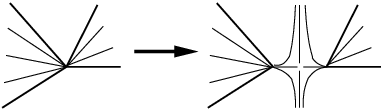
By a -small isotopy of the surface one can remove a hyperbolic and an elliptic singularity which are connected by a leaf of if the signs of the singularities agree. The characteristic foliation before the isotopy is depicted in Figure 4. The segment corresponds to the thickened segment in the middle of Figure 4.
After the elimination of a pair of singularities as in Lemma 3.5 the characteristic foliation on a neighbourhood of looks like in Figure 5.

The elimination of singularities plays an important role in Eliashberg’s proof of Theorem 1.6 for tight contact structures.
Below we give a proof of the elimination lemma which applies to confoliations under a condition on the location of the singularities. Usually the elimination lemma is proved using Gray’s theorem but this theorem is not available in the current setting (this is explained in [1] for example).
Lemma 3.5.
Let be a surface in a confoliated manifold . Assume that the characteristic foliation on has one hyperbolic singularity and one elliptic singularity of the same sign which are connected by a leaf of the characteristic foliation.
If the elliptic singularity lies in , then then there is a -small isotopy of with support in a small open neighborhood of such that the new characteristic foliation has no singularities inside of . The isotopy can be chosen such that is contained in the isotoped surface.
Note that if is a foliation, then the situation of the lemma cannot arise since all leaves of the characteristic foliations in a neighbourhood of an elliptic singularity are closed.
Proof of Lemma 3.5.
We assume that both singularities are positive. There is a neighbourhood of with coordinates such that is defined by the -form such that the function satisfies . We assume that is positively transverse to and , and the axis of the coordinate system contains .
It follows that can be extended to a confoliation on which satisfies the assumptions of Lemma 2.1 if is a ball and is tangent to along a circle. Since every step in the proof will take place in a fixed small neighbourhood of we can apply Lemma 2.1 without any restriction. We choose so that for all in a neighbourhood of . For a path we will consider the hypersurface . By our choices is transverse to the second factor of .
Choose a smooth foliation of a small neighbourhood (contained in ) of in by intervals as indicated by the dashed lines in Figure 4. We choose such that it has the following properties.
- (i)
Two intervals pass through the singularities. One of them is tangent to the closure of the unstable separatrices of the hyperbolic singularity.
- (ii)
All intervals intersecting the interior of have exactly two tangencies with the characteristic foliation on . The intervals which do not intersect the closure of are transverse to the characteristic foliation.
- (iii)
Let by a path in which is shorter than with respect to a fixed auxiliary Riemannian metric. If is small enough, then the image of under the holonomy along is defined. We assume that the length of each is smaller than .
We parameterize the leaf by such that the intersection of with is positive (or empty), ie. in Figure 4 the leaves of are oriented towards the upper part of the picture.
The following figures show neighbourhoods of in for certain . In each of these figures the dotted line represents , oriented from left to right. Figure 6 corresponds to a leaf which does not intersect . Then is nowhere tangent to the characteristic foliation on . By our orientation conventions and the choice of the slope of is negative along .
The leaves contain the singular points of the characteristic foliation on . As shown in Figure 7 there is exactly one tangency of and the characteristic foliation on . The slope of the characteristic foliation on is negative along except at the point of tangency.

Finally, the leaves intersect the interior of and is tangent to in exactly two points. This is shown in Figure 8. Between the two points of tangency, the slope of the characteristic foliation on is positive along , it is zero at the tangencies and negative at the remaining points of .
We want to find a smooth family of isotopies of the intervals within such that
- (i)
for all the isotopy is constant near the endpoints of and
- (ii)
after the isotopy, the intervals are transverse to the characteristic foliation on .
This will produce the desired isotopy of . Such a family of isotopies exists if and only if the following condition (s) is satisfied for all :
Condition (s): The image of under the holonomy along lies below the other endpoint of or the leaf of which passes through exits through .
Note that this condition is automatically satisfied for if does not intersect or this intersection point is close enough to a singularity of the characteristic foliation.
If (s) is not satisfied for all , then we will replace by another foliation by intervals (the corresponding embeddings of intervals are denoted by ) as follows:
- (i)
If does not intersect , then . intersects if and only if does.
- (ii)
is tangent to the characteristic foliation on along two closed intervals (which may be empty or points). The complement of these two intervals is the union of three intervals such that each of these intervals is mapped to a curve of length .
- (iii)
and coincide on those intervals where the characteristic foliation on has negative slope for all .
- (iv)
bounds a positively oriented disc (here denotes the interval with the opposite orientation).
In Figure 9 the dashed line corresponds to while the thick solid line represents .

For we define a curve by replacing the segment of lying between the tangencies with by two segments of leaves of whose -limit set is the elliptic singularity in . Then the holonomy on clearly satisfies the condition (s). This shows that for each one can choose with the desired properties.
Moreover, whenever satisfies (s) then so does by Lemma 2.1. It follows that we can choose the foliation such the leaf of satisfies (s) for all . The desired isotopy of can be constructed such that the surface is transversal to throughout the isotopy. ∎
The following lemma is a partial converse of the elimination lemma. Because is only concerned with the region where is a contact structure we omit the proof. It can be found in [8, 14].
Lemma 3.6.
Let be an embedded surface in a confoliated manifold and a compact segment of a nonsingular leaf of the characteristic foliation on which lies in the contact region of .
Then there is a -small isotopy of with support in a little neighbourhood of such that after the isotopy there is an additional pair of singularities (one hyperbolic and ons elliptic) having the same sign. The isotopy can be performed in such a way that is still tangent to the characteristic foliation and connects the two new singularities.
We end this section with mentioning a particular perturbation of an embedded surface which also appears in [8]. Consider an injective Legendrian polygon such that there is an elliptic singularity of such that consists of more than one vertex of .
Then can be deformed by a -small isotopy near into a surface such that there is a map with the same properties as which coincides with outside a neighbourhood of and maps all vertices in to different elliptic singularities of , cf. Figure 10.
3.4. Modifications in the neighbourhood of integral discs
The second method for the manipulation of the characteristic foliation on an embedded surface is by surgery of the surface along a cycle which is part of an integral disc of . The latter condition is satisfied when the confoliation is tight and bounds a disc in (for example when is simply connected).
While the elimination lemma is used in the proof of the Thurston-Bennequin inequalities for embedded surfaces in tight contact manifolds, the following lemmas adapt lemmas appearing in [26, 28] (cf. also [4]) which are used in the proof the the existence of the Roussarie-Thurston normal form for surfaces in -manifolds carrying a foliation without Reeb components. The existence of this normal forms implies the Thurston-Bennequin inequalities for such foliations.
Lemma 3.7.
Let be a surface and a closed leaf of the characteristic foliation on such that there is a disc tangent to which bounds and has .
Then there is a surface which is obtained from by removing an annulus around and gluing in two discs . The discs can be chosen such that the have exactly one elliptic singularity in the interior of .
If the germ of the holonomy has non trivial holonomy along on one side of , then we can achieve that the elliptic singularity on the disc on that side lies in the interior of the contact region and every leaf of the characteristic foliation on the new discs connects the singularity with the boundary of the disc.
Proof.
We will construct the upper disc in the presence of non-trivial holonomy on the upper side of . The construction of the other disc is analogous.
Fix a closed neighbourhood of such that the fibers of are positively transverse to . We assume and we identify with the unit disc in .
By Lemma 2.1 there is and such that is contained in the interior of the contact region of . On we consider the singular foliation consisting of straight lines starting at . For let be the disc formed by horizontal lifts of leaves of the singular foliation on with initial point . By Gray’s theorem we may assume that is generic near . Then is homeomorphic to the singular foliation by straight lines on and the singularity is non-degenerate for all .
Let be a monotone function which is smooth on such that near and the graph of is -tangent to a vertical line at . We denote the boundary of the disc of radius in by . The union of all with the part of which corresponds to the disc with radius is the desired disc . We remove the annulus from and add .
By construction the only singular point of is , the singularity is elliptic and contained in the contact region. Its sign depends on the orientation of .
In order to show that all leaves of accumulate at the elliptic singularity it is enough to show that there are no closed leaves on . Assume that is a closed leaf of . Let be the disc formed by lifts of the leaves of the radial foliation on with initial point on .
The restriction of to extends to a confoliation on which is a complete connection. By Proposition 2.5 is tight. Hence must bound an integral disc of . Now is the only possible candidate for such a disc. But cannot be an integral disc of because it intersects the contact region of (or equivalently ) in an open set. This contradiction finishes the proof. ∎
The following two lemmas are analogues to the elimination lemma in the sense that we will remove pairs of singularities. Note however that new singularities can be introduced. In particular in Lemma 3.9 we will obtain a surface whose characteristic foliation is not generic. However this will play no role in later applications since the locus of the non-generic singularities will be isolated from the rest of the surface by closed leaves of the characteristic foliation.
Lemma 3.8.
Let be a surface in a confoliated manifold, an embedded disc tangent to and is a cycle containing exactly one hyperbolic singularity .
Then there is a surface which coincides with outside of a neighbourhood of and is obtained from by removing a tubular neighbourhood of and gluing in two discs . The characteristic foliation of has no singularities on and one elliptic singularity on whose sign is the opposite of the sign of .
Proof.
The assumptions of the lemma imply that has a stable and an unstable leaf which do not lie on .
Choose a simple curve connecting to another boundary point of such that is not tangent to a separatrix of and extend to a Legendrian curve such that become an interior points of . Fix a product neighbourhood of with the following properties.
- (i)
is contained in the interior of the disc .
- (ii)
There is a simple Legendrian curve containing in its interior and intersecting respectively in two points such that is nowhere tangent to respectively is transverse to .
- (iii)
The fibers of the projection are transverse to .
Now consider . The intersection has a non-degenerate tangency with in and meets transversely in . We choose two points such that lie between and , as indicated in Figure 11.

The points can be connected by a curve transverse to the characteristic foliation on this strip provided that are close enough to . Moreover, we may assume that is tangent to near its endpoints (cf. the lower dashed curve in Figure 11).
The curve is going to be part of . In order to finish the construction of we choose a foliation of by a family of intervals that connect boundary points of and are transverse to . The characteristic foliation on consists of lines which are mapped diffeomorphically to by .
If was chosen close enough to , then there is a smooth family of curves in which
- (i)
intersect and are tangent to in these points,
- (ii)
are transverse to elsewhere and
- (iii)
are tangent to near .
The choices we made for and ensure that the union of all curves is a disc which is transverse to .
The disc is obtained as in the proof of Lemma 3.7. The statement about the sign of the singularity of follows from the construction. ∎
Lemma 3.9.
Let be an embedded surface in a manifold carrying a confoliation such that contains a hyperbolic singularity and the stable and unstable leaves of bound an annulus which is pinched at . We assume that the pinched annulus is bounded by an integral disc of such that .
Then there is an embedded surface which is obtained from by removing a neighbourhood of and gluing in an annulus and a disc such that has one of the following properties.
- (i)
has no singularity.
- (ii)
The singularities of form a circle and a neighbourhood in of this circle is foliated by closed leaves of .
The characteristic foliation on has exactly one singularity which is elliptic and whose sign is opposite to the sign of .
Proof.
The disc in the statement of the lemma is an immersed disc which is an embedding away from two points in the boundary. These two points are identified to the single point . Let be a simple closed curve in which meets exactly once.
We choose a solid torus such that and the foliation corresponding to the second factor is Legendrian while the foliation corresponding to the third factor is transverse to . For let . The torus is chosen such that and intersects in two circles while is a circle which bounds is disc in .
If is thin enough, then a disc which bounds with the desired properties can be constructed as in the proof of Lemma 3.7.
Let . The characteristic foliation on consists of lines transverse to the last factor of and is a leaf of
If one of the annuli has non-trivial holonomy along or if is not Legendrian, then one can choose a curve in that annulus which is transverse to . The annulus is the union of curves in which connect the two points of and pass through . These curves can be chosen such that they are transverse to everywhere except in . By construction has the property described in (i) of the lemma.
This construction also applies if we choose in annuli which are -close to for a suitable . If all annuli of this type have trivial holonomy along their boundary curve which is close to , then is a foliation on a neighbourhood of in by Lemma 2.1 whose holonomy along is trivial. The same construction as in the previous case (with ) yields an annulus with the properties described in (ii). ∎
Lemma 3.7 and Lemma 3.8 suffice for Section 5 because the embedded surfaces in that section are going to be simply connected. Then one can apply Lemma 3.8 to one of the boundary components of the pinched annulus.
In the lemmas of this section we have assumed that . In general and may intersect elsewhere. Since all singularities of the characteristic foliation on are non-degenerate or of birth-death type, there is a neighbourhood of in such that is the intersection of with this neighbourhood. After a small perturbation with support outside of a neighbourhood of we may assume that is transverse to on the interior of . Now we can apply Lemma 3.7 a finite number of times to circles in in order to achieve that the resulting surface intersects only along . Then we can apply the lemmas of this section.
4. Tight confoliations violating the Thurston-Bennequin inequalities
The example given in this section shows that tightness (as defined in Definition 1.3) is a much weaker condition for confoliations compared to the rigidity of tight contact structures or foliations without Reeb components. It also shows that it may happen that every contact structure obtained by a sufficiently small perturbation of a tight confoliation is overtwisted. This is in contrast to the situation of foliations without Reeb components: According to [7] every foliation without a Reeb component can be approximated by a tight contact structure.
The starting point for the construction of a tight confoliation violating the Thurston-Bennequin inequalities is the classification of tight contact structures on such that the characteristic foliation on is linear (cf. [15]). We fix an identification and the corresponding vector fields .
According to [15] (Theorem 1.5) there is a unique tight contact structure on such that
- (i)
the characteristic foliation on is a pair of linear foliations whose slope is respectively on respectively ,
- (ii)
the obstruction for the extension of the vector fields which span the characteristic foliation on is Poincaré-dual to .
Figure 12 shows the characteristic foliation on at various times and its orientation. The two curves in where the characteristic foliation is singular represent the homology class .
We may assume that the contact structure is -invariant and tangent to on a neighbourhood of the boundary (cf. [14]). Then there are smooth functions on this neighbourhood such that is spanned by and
| (4) | ||||
Because is a positive contact structure, the functions satisfy the inequalities for on their respective domains.
We now modify to a confoliation on . For this replace the functions in (4) by such that for
- •
coincide with outside of small open neighbourhoods of
- •
there is such that if and
- •
for
- •
coincide with at .
Remark 4.1.
From the proof of Theorem 1.5 in [15] it follows that the contact structure on is tight.
We write for the confoliation constructed so far. In the next step we will extend to a smooth confoliation on such that the boundary consists of torus leaves.
Let be a diffeomorphism of such that for and all derivatives of vanish for . The suspension of this diffeomorphism yields a foliation on whose only closed leaf is and all other leaves accumulate on this leaf. In this way we obtain a foliation on such that the boundary is a leaf and the characteristic foliation on corresponds to the first factor. In particular it is linear.
Using suitable elements of we glue two copies of the foliation on to . We obtain an oriented confoliation on such that the boundary is the union of two torus leaves and we may assume the orientation of the boundary leaves coincides with the orientation of the fiber of .
After identifying the two boundary components by an orientation preserving diffeomorphism, we get a closed oriented manifold carrying a smooth positive confoliation which we will denote again by .
Claim: is tight.
We show that the assumption of the contrary contradicts Remark 4.1. Let be a Legendrian curve which bounds an embedded disc in such that is nowhere tangent to along and violates the requirements of Definition 1.3. By construction has a unique closed leaf . If is contained in , then bounds a disc in because is incompressible. Thus we may assume that lies in the complement of and we can consider the manifold .
By Remark 4.1, cannot be contained in . If lies completely in the foliated region , then it bounds a disc in its leaf because all leaves are incompressible cylinders.
It remains to treat the case when the intersects the contact region and the foliated region. All leaves of in are cylinders which can be retracted into the region . Hence we may assume that is contained in .
First we show that there is a Legendrian isotopy of such that the resulting curve is transverse to the boundary of the contact region . A similar isotopy will be used later, therefore we describe it in detail.
Let with be a neighbourhood of one component of where can be defined by the -form
We consider the projection such that the fibers are tangent to . Note that is the lift of the -form
The fibers of are transverse to . Let be a segment of which is contained in and whose endpoints do not lie on .
If is contained in the foliated part of , then we isotope within its leaf such that the resulting curve is disjoint from and the isotopy does not affect the curve on a neighbourhood of its endpoints.
Now assume that some pieces of are contained in the contact region of . Then passes through the region of where is non-vanishing. We consider an isotopy of the projection of which is fixed near the endpoints and the area of the region bounded by is zero for all curves in the isotopy. By Stokes theorem this implies that one obtains closed Legendrian curves when is replaced by horizontal lifts of curves of the isotopy (with starting point on ).
Hence we may assume that is transverse to and is decomposed into finitely many segments whose interior is completely contained in either the contact region or the foliated region of .
Let be an arc with endpoints in the contact region of such that contains a exactly one sub arc of lying in the foliated region. Because is embedded, it bounds a compact half disc in a leaf tangent to and we can choose such that the half disc does not contain any other segment of .
Now we isotope relative to its endpoints such that after the isotopy this segment lies completely in the contact region of . As above we deform through immersions such that the resulting arc has the following properties
- •
the integral of over the region bounded by and is zero and the same condition applies to every curve in the isotopy,
- •
is completely contained in .
Then the horizontal lift of can be chosen to have the same endpoints as and we can replace by this horizontal lift. The resulting curve is Legendrian isotopic to but it the number of pieces which lie in the foliated region has decreased by one.
After finitely many steps we obtain a Legendrian isotopy between and a closed Legendrian curve which lies completely in the interior of the contact region. The Thurston-Bennequin invariant of the resulting curve is still zero. But this is impossible because the contact structure on is tight.
Claim: If , then violates b) of Theorem 1.6.
The trivialization of induced by the characteristic foliation on extends to the complement of in . The obstruction for the extension of the trivialization from to is Poincaré-dual to . Hence is Poincare-dual to where the second factor corresponds to the homology of the second factor of . This means that violates the Thurston-Benneuqin inequalities since these inequalities imply because every homology class in can be represented by a union of embedded tori.
An example of a torus in which violates the Thurston-Bennequin inequality can be described very explicitly. Let be the torus which is invariant under the -action transverse to the fibers and it intersects each fiber in a curve of slope , hence this curve represents when is suitably oriented. It follows from the description of given above, that is Legendrian and the characteristic foliation on has exactly four singular points which lie on and have alternating signs.
Moreover, is a Legendrian curve and is transverse to all tori except in the singular points on . Figure 13 shows a singular foliation homeomorphic to the one on .

We choose the orientation of such that . In order to find an example of a surface with boundary which violates the inequality c) from Theorem 1.6 it suffices to remove a small disc containing one of the elliptic singularities in .
Finally, note that according to [9] every positive confoliation can be approximated (in the -topology) by a contact structure, it follows that tightness is not an open condition in the space of confoliations with the -topology. Actually can be approximated by contact structures which are -close to . This can be seen by going through the proof of Theorem 2.4.1 and Lemma 2.5.1 in [9]: By construction the holonomy of the closed leaf on is attractive, therefore it satisfies conditions which imply the conclusion of Proposition 2.5.1, [9] (despite of the fact that the infinitesimal holonomy is trivial). The main part of this lemma is stated in Lemma 6.3 together with an outline of the proof.
5. Rigidity results for tight confoliations
The example from the previous section shows that tight confoliations are quite flexible objects compared to tight contact structures and foliations without Reeb components. In this section we establish some restrictions on the homotopy class of plane fields which contain tight confoliations.
The first restriction is the Thurston-Bennequin inequality for simply connected surfaces. Note that this imposes no restriction on the Euler class of a tight confoliation on a closed manifold unless the prime decomposition of contains -summands. The second restriction on the homotopy class of is a consequence of
Theorem 5.1.
Let be a manifold carrying a tight confoliation and a closed embedded ball in . There is a neighbourhood of in the space of plane fields with the -topology such that is tight for every contact structure in this neighbourhood.
The proof of this theorem is given in Section 5.2. Let us explain an application of Theorem 5.1 which justifies the claim that Theorem 5.1 is a rigidity statement about tight confoliations.
By Theorem 1.1 every confoliation on a closed manifold can be -approximated by a contact structure unless it is a foliation by spheres. Hence Theorem 5.1 can be applied to every confoliation. Recall the following theorem.
Theorem 5.2 (Eliashberg, [8]).
Two tight contact structures on the -ball which coincide on are isotopic relative to .
It follows from this theorem that two tight contact structures on are isotopic and therefore homotopic as plane fields. In contrast to this every homotopy class of plane fields on contains a contact structure which is not tight. Thus the following consequence of Theorem 5.1 shows that there are restrictions on the homotopy classes of plane fields containing tight confoliations.
Corollary 5.3.
Only one homotopy class of plane fields on contains a positive tight confoliation.
Proof.
Let be a tight confoliation on . It is well known that every foliation of rank on contains a Reeb component, cf. [24]. Thus is not empty. We choose and a ball around .
More generally, Theorem 5.1 together with Theorem 5.2 implies that the homotopy class of a tight confoliation as a plane field is completely determined by the restriction of to a neighbourhood of the -skeleton of a triangulation of the underlying manifold.
5.1. The Thurston-Bennequin inequality for discs and spheres
In this section we prove the Thurston-Bennequin inequalities for a tight confoliation in the cases where is a sphere or a disc (with transverse boundary). For this we adapt the arguments in [8]. We shall discuss why Eliashberg’s proof cannot be adapted for non-simply connected surfaces in tight confoliations after the proof Theorem 5.4. Recall that the self-linking number of a null-homologous knot which is positively transverse to with respect to a Seifert surface satisfies where corresponds to the obstruction for the extension the characteristic foliation near to a trivialization of .
Theorem 5.4.
Let be a manifold with a tight confoliation. Then
- a)
for every embedded -sphere and
- b)
for every embedded disc whose boundary is positively transverse to .
Proof.
We perturb the surface such that it becomes generic and the elliptic singularities lie in the interior of or in the interior of the foliated region. Furthermore, we will assume in the following that there are no connections between different hyperbolic singularities of characteristic foliations.
We show for every disc as in b). By the Poincaré index theorem
| (5) | ||||
Subtracting these equalities we obtain . In order to prove the b) it suffices to replace by an embedded disc with such that contains no negative elliptic singularities.
Because is tight and is simply connected each cycle of is the boundary of an integral disc. We can apply Lemma 3.7 or Lemma 3.8 to such discs to obtain a new embedded disc . By (iii) of Definition 1.3 .
We now choose particular cycles of to which we apply Lemma 3.7 and Lemma 3.8: Define for two cycles of the characteristic foliation if bounds an embedded disc containing . We apply Lemma 3.7 and Lemma 3.8 to cycles which are maximal with respect to . This means in particular that the holonomy of maximal cycles which are closed leaves of is not trivial on the outer side of the cycle.
Hence we obtain a disc whose characteristic foliation does not have closed cycles and all elliptic singularities are contained in . In particular there are no integral discs of which pass though elliptic singularities of the characteristic foliation of . Moreover, . From now on we will write instead of .
Adapting arguments from [8] we eliminate one negative elliptic singularity . Let be a disc such that is transverse to and . According to Lemma 3.4 there is a Legendrian polygon covering . In the present situation since has no cycles or exceptional minimal sets. Note that because the characteristic foliation is pointing outwards along . After a small perturbation of we may assume that identifies vertices of only if adjacent edges are also identified, for elliptic vertices this is illustrated in Figure 10. In this situation all boundary components of are embedded piecewise smooth circles.
Recall that contains no cycles. Then every boundary component of therefore contains an elliptic singularity (which has to be positive). If all singularities of on are positive, then we obtain a contradiction to the tightness of . Hence contains a negative singularity which has to be hyperbolic. According to our assumptions it is a pseudovertex of the Legendrian polygon, ie. its unstable leaf ends at while the other unstable leaf never meets .
Therefore the application of the elimination lemma (Lemma 3.5) does not create new cycles on the disc. We continue with the elimination of negative elliptic singularities until . This finishes the proof of b)
Now we come to the prove of a). First we use Lemma 3.7 and Lemma 3.8 in order to decompose into a disjoint union of embedded spheres such that there are no cycles which contain hyperbolic singularities. In the following we consider each sphere individually, so we continue to write . If contains a closed leaf, then the claim follows immediately from the definition of tightness: Let be the two discs with . Then there is an integral disc of such that . We orient such that is a cycle and denote by the disc with the opposite orientation. Then and the claim follows from (iii) of Definition 1.3 applied to :
Finally if has neither closed leaves or cycles, then one can prove a) using b) when one considers complements of small discs around positive or negative elliptic singularities. ∎
Consider a Legendrian polygon in when is a contact structure on . Generically the characteristic foliation on is of Morse-Smale type (cf. [14]). In particular there are no quasi-minimal sets. If the set of virtual vertices of the Legendrian polygon associated to is not empty, then by Lemma 3.6 one can create of a canceling pair of singularities along on for such that all leaves which accumulated on now accumulate on an elliptic or a hyperbolic singularity.
For this reason the case plays essentially no role when is a contact structure. If the -limit set of is contained in the fully foliated part of , then it not possible to apply Lemma 3.6 (cf. Section 4). It is at this point where the proof of the Thurston-Bennequin inequalities for tight contact structures fails when one tries to adapt the arguments from [8] to tight confoliations and surfaces which are not simply connected.
We finish this section with a remark that will be useful later.
Remark 5.5.
Let be a tight confoliation. For an embedded surface we define for open subsets of . Note that if is a sphere, then by Theorem 5.4 and .
Part b) Theorem 5.4 can be strengthened: It is not only possible to replace be a disc with the same boundary and such that has no negative elliptic singularities. Consider -limit set of stable leaves of positive hyperbolic singularities of . Since contains no cycles the -limit set is generically a positive elliptic singularity. Thus we may eliminate all negative elliptic and all positive hyperbolic singularities from . This implies the following inequalities:
In a later application we shall consider discs such that is negatively transverse to . Then the two inequalities above will be interchanged.
5.2. Perturbations of tight confoliations on balls
The proof Theorem 5.1 is given in the following sections. It has two main ingredients: First we generalize taming functions on spheres to confoliations. We show that the characteristic foliation on an embedded sphere can be tamed if is tight and that this remains true for contact structures which are close enough to . Then we apply arguments from [15] to conclude that is tight if is a contact structure.
In the following sections will always be an oriented tight confoliation on and denotes an embedded oriented sphere. We do not consider foliations by spheres.
5.2.1. Properties of characteristic foliations on spheres
The tightness of leads to restrictions on the signs of hyperbolic singularities on . Lemma 5.8 is concerned with signs of hyperbolic singularities on cycles of when is a tight confoliation. To state it we need the following definition:
Definition 5.6.
A cycle connected of is an internal subcycle if there is another cycle of such that is not empty and the integral disc which bounds contains the integral disc which bounds .
A leaf of is called internal if there are two cycles of which bound discs tangent to whose interiors are disjoint. We say that a hyperbolic singularity on is essential if it is not lying on an internal subcycle of .
The union of singular points and cycles of will be denoted by . This set is compact.
An example of an internal subcycle is shown in Figure 14. Note that one can create internal cycles intersecting a fixed cycle of with arbitrary sign using an inverse of the construction explained in Lemma 3.8.
If a connected cycle of contains hyperbolic singularities, then the holonomy along can be defined at most on one side. The one-sided holonomy is defined if and only if there is an immersion of a disc into which is an embedding on and is mapped onto such that the image of does not contain a stable or unstable leaf of a hyperbolic singularity on . We will say that is a disc in although some points on the boundary may be identified.
The singularities on can be decomposed into two classes
Let be a cycle of and a disc with whose interior does not contain a stable leaf of a hyperbolic singularity on . Then the one-sided holonomy along is well defined. Because is tight there is a disc tangent to such that . We orient using the orientation of .
Definition 5.7.
We say that is potentially attracting if
- (i)
lies below respectively above (with respect to the coorientation of ) in a neighbourhood of and
- (ii)
the orientation of is opposite respectively equal to the orientation of .
In the opposite case, is potentially repulsive.
According to Lemma 2.1 the holonomy along potentially repulsive respectively attractive cycles is non-repelling respectively non-attracting. The terminology of Definition 5.7 is introduced to deal with the case when the holonomy is trivial (and therefore non-repelling and non-attracting at the same time).
Lemma 5.8.
Let be a cycle of containing a hyperbolic singularity and such that the one-sided holonomy is defined.
Then all essential singularities in have the same sign and all essential singularities in have the opposite sign. The one-sided holonomy is potentially attractive (respectively repulsive) if and only if all singularities in are negative (respectively positive) and all singularities in are positive (respectively negative).
The signs of the non-essential singularities in respectively is opposite to the sign of the essential singularities in respectively .
Proof.
Let be the disc in with such that the one-sided holonomy is defined on the side of where is lying. Because is tight, there is a disc tangent to which bounds . Consider a tubular neighbourhood of which contains a collar of and the collars lies on one side of in the tubular neighbourhood.
The statement about the signs of singularities now follows by looking how approaches near the tangencies and the relation between the signs and the holonomy is a consequence of our orientation conventions and Lemma 2.1. ∎
The following proposition is a generalization of Lemma 4.2.1 in [8]. It will play an important role in the proof of Theorem 5.1.
Proposition 5.9.
Let be a tight confoliation on and an embedded sphere such that the singularities of are non-degenerate. Let be a connected submanifold of dimension such that is transverse to and points outwards along . Each connected component of the boundary the associated Legendrian polygon has the following properties.
- (i)
If there is a negative elliptic singularity on such that is not a neighbourhood of or a cycle with such that is not a one-sided neighbourhood of , then contains a positive pseudovertex.
- (ii)
If and identifies the edges of , then maps the pseudovertices on to negative hyperbolic singularities of .
Proof.
It was shown in Lemma 3.4 that is covered by a Legendrian polygon . Recall that is defined only on , but we shall denote by .
First we reduce the situation to the case when . By the theorem of Poincaré-Bendixon, the -limit sets corresponding to points of are cycles. Because is tight, these cycles bound integral discs of and we can apply Lemma 3.7 or Lemma 3.8. Since the discs bounding these cycles may intersect it is also necessary to consider cycles in .
Let and the integral disc of which bounds and a cycle of which is contained in . We assume that the disc bounded by intersects only along . The cycle is either contained in or in the complement of .
We begin with the case . In this case we obtain two embedded spheres by cutting along . When we use Lemma 3.7 for this the subset induces two subsets such that respectively contains one positive respectively one negative singularity in addition to singularities which were already present in , respectively is transverse to respectively and the characteristic foliation points outwards. The pseudovertices of the Legendrian polygons associated to the basins of coincide with the pseudovertices of . If , then
| (6) | ||||
Notice that and is negatively transverse to . It follows from Remark 5.5 that and . Together with (6) this implies .
If we applied Lemma 3.8 and the hyperbolic singularity was positive respectively negative, then respectively and one of the sets, say coincides with . Then implies .
When lies in the complement of , cutting along will not affect or but the basin of can change: We might remove a virtual vertex, or after the surgery process some boundary components of the Legendrian polygon might be mapped to a negative elliptic singularity while they were accumulated on a cycle before. The pseudovertices are not affected. Note also that if is a one–sided neighbourhood of a cycle , then the Legendrian polygon which results from the surgery along will be a neighbourhood of the negative elliptic singularity which results from surgery process. (Recall that has well defined attractive one–sided holonomy on the side of ).
After finitely many steps we obtain a finite union of embedded spheres and subsets with the same properties as such that the associated Legendrian polygon satisfies . Therefore is suffices to prove the claim when is covered by a Legendrian polygon with . Let be a boundary component of .
We now prove (i). Let be an elliptic singularity such that is not a neighbourhood of . Then the connected component of containing is a piecewise smooth closed curve . After a perturbation of the sphere we may assume that does not contain corners, and is embedded (cf. Figure 10). If all singularities on were negative, then we would get a contradiction to the tightness of since no integral surface of can meet . Since all elliptic singularities on are attractive and therefore negative there must be a positive pseudovertex on .
It remains to prove (ii). Assume and let be the pseudovertices on the edges .
When for , then . Let be the two stable leaves of . After a small perturbation of in the complement of we may assume that the -limit sets of are contained in .
If for all , then let be two hyperbolic singularities which lie on the cycle associated to identified edges (cf. Definition 3.3) and are connected by a piecewise smooth simple oriented path in the complement of consisting of leaves of and hyperbolic singularities (as corners) such that starts at and ends at without passing through images of other pseudovertices. After a small perturbation of in the neighbourhood of we obtain a sphere such that the -limit sets of the two stable leaves of are contained in .
We may assume that neither or is a hyperbolic singularity or a singularity of birth-death type. By the Poincaré-Bendixon theorem is either an elliptic singularity or a cycle. The same is true for . Using Lemma 3.7 and Lemma 3.8 we can ensure that is an elliptic singularity, which has to be positive. Note that lie in the same connected component of the two spheres obtained by the surgery along cycles in .
For the same reason we may assume that the -limit set of each stable leaf of hyperbolic singularities in is an elliptic singularity in . Under these conditions the hypotheses implies that the graph formed by positive singularities (except birth-death type singularities) and stable leaves of hyperbolic singularities is a connected tree.
Both stable leaves of together with the simple path on the tree connecting with form a simple closed curve on which is Legendrian. All singularities on except are positive by construction. Moreover, contains an elliptic singularities which lies in . If is positive we obtain a contradiction to the tightness of since cannot bound an integral disc of . ∎
In order to apply the previous proposition efficiently it remains to show that either one of the two parts of Proposition 5.9 can be used or does not contain any pseudovertices at all. This is done in the following lemma.
Lemma 5.10.
In the situation of Proposition 5.9 has more connected components or one of the following statements holds for each connected component of .
- (i)
There is a connected component of such that is an elliptic singularity and is a neighbourhood of or is a cycle and is a one-sided neighbourhood of that cycle.
- (ii)
contains a cycle of such that is not a one-sided neighbourhood of or contains an elliptic singularity such that is not a neighbourhood of .
- (iii)
identifies edges on .
Proof.
After a small perturbation of we may assume that all negative elliptic singularities on lie in or the interior of the complement of . As in the proof of the previous proposition the problem can be reduced to the case when .
We show that if (i) and (ii) do not hold for , then (iii) applies to . In the following discussion we ignore corners on if two of their separatrices lie in the complement of .
Let be an elliptic singularity. Since there is an unstable leaf of a pseudovertex which ends at . Let be the other unstable leaf of .
If the -limit set of is a negative elliptic singularity, then is contained in the interior of and the two edges of which correspond to are identified by . Otherwise the -limit set of is a hyperbolic singularity and we can assume that is a pseudovertex of . There is a unique unstable leaf of which is not contained in the interior of . In particular the -limit set of cannot by an elliptic singularity. Thus the -limit set of is the image of a pseudovertex of . If , then identifies the edges corresponding to and form a non-trivial cycle of .
Otherwise we continue as above until a pseudovertex appears for the second time. This happens after finitely many steps since contains only finitely many pseudovertices. If we obtained a sequence with , then identifies the edges corresponding to the pseudovertices . Thus if (i) and (ii) do not apply, then (iii) is true. ∎
5.2.2. Taming functions for characteristic foliations on spheres
Taming functions for characteristic foliations were introduced by Y. Eliashberg in [8]. In this section we extend the definition of taming functions so that it can be applied to spheres embedded in manifolds carrying a tight confoliation.
Let be an embedded sphere in a confoliated manifold such that the singularities of the characteristic foliation are non-degenerate or of birth-death type. This assumption holds in particular for spheres in a generic -parameter family of embeddings. In addition we may assume that there are at most two different hyperbolic singularities which are connected by their stable/unstable leaves.
Definition 5.11.
Let be a compact submanifold of dimension in whose boundary is piecewise smooth and does not intersect . Moreover, we assume that every connected component satisfies one of the following conditions:
- (1)
is either transverse or tangent to .
- (2)
intersects one respectively two stable leaves of hyperbolic singularities of (these singularities may be part of a cycle, cf. Figure 15 or is a neighbourhood of a hyperbolic singularity). Each smooth segment of intersects exactly one separatrix of a hyperbolic singularity in and each segment is transverse to .
- (3)
is disc and a neighbourhood of a birth-death type singularity of such that consists of two smooth segments transverse to .
A function is a taming function for if it has the following properties.
- (o)
If a component belongs to the class (1), then is assumed to be constant along . If is of class (2) or (3) we require that has exactly one critical point in the interior of each of the smooth segments of .
- (i)
The union of the singular points of with all points on internal leaves coincides with the set of critical points of . The function is strictly increasing along leaves of which are not part of a cycle and is constant along cycles of .
- (ii)
Positive respectively negative elliptic points of are local minima respectively maxima of .
- (iii)
If the level set contains only hyperbolic singularities, then as increases the number of closed connected components of changes by .
Requirement (i) in Definition 5.11 is slightly more complicated than one might expect. Figure 14 gives an example of a sphere in equipped with the foliation by horizontal planes. A part of the characteristic foliation is indicated in the right part of Figure 14 where the cycle containing the internal subcycle is thickened. If one requires that singular points of should coincide with critical points of the taming function, then cannot be tamed although the confoliation in question is tight.

Assume that is a symplectic filling of and a compatible almost complex structure on is fixed such that consists of complex lines. By Theorem 1 of [18] an embedded -sphere can be filled by holomorphic discs when the embedding of satisfies several technical conditions. The singular foliation in the formulation of Theorem 1 in [18] is very similar to the singular foliation formed by level sets of a taming function. The appearance of internal cycles should be compared with Remark 2 in [18].
5.2.3. Construction and deformations of taming functions
Let an embedded oriented -sphere. The tightness of leads to several restrictions on the combinatorics of the cycles of and their holonomy. This will be used to construct a taming function for .
Recall that the orientations of and induce an orientation of and integral surfaces of are oriented by . If is a cycle of , then by tightness there is an integral disc of such that but the orientation of as boundary of does not coincide with the orientation of in general. Recall also that is uniquely determined because is not a foliation by spheres.
For a -dimensional submanifold with piecewise smooth boundary we define the following quantities:
| stable leaves of negative hyperbolic singularities enter. | |||
These quantities will be used in the construction of taming functions.
Lemma 5.12.
For each path connected component of there is a neighbourhood of and a taming function such that no connected component of is tangent to and
| (7) |
Proof.
We will construct and inductively. The starting point are connected cycles and singularities of in which belong to the following classes.
- (i)
Positive elliptic singularities and hyperbolic or birth-death type singularities which do not belong to a cycle.
- (ii)
Closed leaves with sometimes attractive (non-trivial) one-sided holonomy.
- (iii)
Cycles containing hyperbolic singularities which satisfy the following conditions:
- –
The only cycle of containing is .
- –
If is a subcycle with potentially attractive one-sided holonomy, then this one-sided holonomy is not trivial.
- –
If the positive elliptic singularity in (i) is dynamically hyperbolic, then it is a source and there is a taming function on a neighbourhood whose boundary is transverse to . If the elliptic singularity is not dynamically hyperbolic, then one obtains a taming function using the holonomy of an interval which is transverse to except at and corresponds (cf. Lemma 3.1). If the holonomy is non-trivial, then we can choose the domain of the taming function such that is transverse to . Otherwise we choose such that is a closed leaf of . Moreover, satisfies (7).
If is a hyperbolic singularity or a singularity of birth-death type, then the existence of a taming function on a neighbourhood which satisfies (7) is obvious.
For a closed leaf of as in (ii) we choose an embedded interval transverse to such that corresponds to a point in and corresponds to the side where the holonomy of is sometimes attractive. This choice determines along the transverse segment and can be extended to a taming function on a neighbourhood of . If the holonomy on the side is non-trivial (respectively trivial) we choose to be an annulus with transverse boundary (respectively such that is a leaf of and the other component of is transverse to ). Thus and contains no singular points of . This means that (7) holds for .
Now let be a cycle containing hyperbolic singularities. For each subcycle with potentially attractive (respectively repelling) one-sided holonomy chose a transversal (respectively ) with lying on and construct taming functions on collars of discs bounding the subcycle. When the germ of the one-sided holonomy is nontrivial, then we can choose the boundary corresponding boundary component of the domain of to be transverse to , otherwise we can choose the boundary of the domain to be tangent to a leaf of .
If contains a corner such that only one stable leaf of the hyperbolic singularity is part of , then the levelsets of near can be chosen as suggested in Figure 15. The thick curve represents a critical level of while the dashed curve corresponds to a regular level of .

By construction is constant along cycles and increasing along leaves of which are not part of cycles. Singular points of clearly are critical points of . In order to show that requirement (i) of Definition 5.11 is satisfied by we consider an internal leaf .
Let be discs which lie on opposite sides of and contain no subcycle of in their interior. Because is an internal leaf respectively can not contain a stable or unstable leaf of a hyperbolic singularity on respectively . Therefore the one-sided holonomy along and is well defined and by Lemma 2.1 the holonomy along is potentially attractive if and only if the same is true for the holonomy along . Hence has a local minimum respectively maximum at every point of when the holonomy is potentially repulsive respectively attractive.
Using induction on the number of hyperbolic singularities in we now prove requirement (iii) from Definition 5.11 and (7) for . We have already treated the case when contains no hyperbolic singularity.
Given a cycle and a fixed hyperbolic singularity we isotope in a neighbourhood of . We choose the isotopy such that segments of in which ended at before the perturbation are now connected be non-singular segments of . In this way obtain a cycle on which contains one singularity less than and it may happen that is not connected.
In order to construct an isotopy with the desired properties one moves away from the integral surface of which contains the cycle . When is part of an internal cycle or not all stable/unstable leaves of are contained in one has to move into the interior of an integral surface of and then slightly above or below the integral surface with respect to the coorientation of . Choosing to push upwards or downwards one can make sure that on obtains a cycle on the perturbed surface which is contained in the interior of the integral surface of which contains . Figure 16 shows one particular instance of the isotopy in a neighbourhood of . In that figure, we move downwards. In the left part of the figure all lines are part of while in the right part they straight line do not belong to . The cycles respectively correspond to the thickened lines in the left respectively right part of Figure 16.
If there is a hyperbolic singularity such that contains only one stable leaf of , then is automatically an essential singularity on and our orientation convention and the choice of the function in Figure 15 together with Lemma 5.8 imply that the behavior of the level sets of near is compatible with requirement (iii) of Definition 5.11.
In order to prove (7) we perturb . After an isotopy of in a neighbourhood of we obtain a cycle which contains one singularity less than and the singularity we removed had a stable leaf which was not part of . We construct the function on as above. When is positive, then
Therefore (7) holds for if and only if it holds for . If is negative we have to distinguish two cases: In the first case, the stable leaf of is the only stable leaf of a negative hyperbolic singularity intersecting the connected component of . Then
If there are other stable leaves of other hyperbolic singularities of which intersect the same connected component of as the stable leaf of , then
Again the validity of (7) for follows from (7) for . For the proof of (7) we may assume from now on that all stable and unstable leaves of all hyperbolic singularities on are contained in . In particular in the sequel.
Let be an essential hyperbolic singularity. We shall discuss the configuration shown in the left part of Figure 16. The other configurations can be handled in the same manner. The vertical arrow in Figure 16 indicates the coorientation of , the other arrows indicate orientations of leaves of and . In addition we assume that the stable leaf on the right (resp. left) hand side is connected in to the unstable leaf on the right (resp. left) hand side.
In this situation is split into two connected components by the isotopy. For both connected components there is an integral disc of which bounds a cycle containing parts of one stable leaf of . The two integral discs have disjoint interiors.
Therefore there is one disc with well defined one-sided holonomy below the integral surface of and and by Lemma 2.1 this holonomy is potentially attractive. There are two discs with well defined one-sided holonomy lying above the integral surface and each of the upper discs contains exactly one stable leaf of in its boundary while the lower disc contains both stable leaves of in its boundary. The one-sided holonomies along the boundary of each of the two discs if potentially repulsive. This is exactly the behavior prescribed by (iii) of Definition 5.11.
We choose neighbourhoods of which satisfy (7). The relation between and is given by
Hence (7) is true for because it is satisfied for . The other configurations can be handled in a similar manner.
Now we assume that is a hyperbolic singularity such that one stable leaf is part of an internal cycle and the other one is part of a subcycle of which is not internal (if there are internal subcycles, then there must be singularities with this property because is connected).
Let be the stable and unstable leaves of which are internal. There is a disc whose boundary contains such that the one-sided holonomy along is well defined. If it is potentially attractive respectively repulsive, then is positive respectively negative by Lemma 5.8.
The remaining pair of separatrices is part of a cycle with well defined one-sided holonomy. It is potentially attractive if and only if the holonomy along is potentially repulsive (cf. Lemma 5.8).
By a small isotopy we can obtain a connected cycle or two connected cycles on the perturbed sphere with one singularity less than such that (ie. the segments lying outside of the support of the perturbation of ) are connected by a leaf of and the same is true for the other pair of separatrices of . Figure 14 shows a cycle which decomposes into a pair of connected cycles. The discussion above shows that satisfies (iii) of Definition 5.11 if the same is true for and .
We construct a taming function on a neighbourhood of the perturbed cycle. The following table summarizes the relations from Lemma 5.8 between the invariants associated to with the invariants for the perturbed cycle.
| is positive | is negative | |||||
|---|---|---|---|---|---|---|
| remains connected |
|
| ||||
| splits into two cycles |
|
|
Therefore (7) holds for the neighbourhood of and has the desired properties.
This finishes the first step in the construction of a taming function on a neighbourhood of . If all components of are transverse to , then and tames on . Otherwise we iterate the above construction.
Assume we have constructed a taming function and is a closed leaf of with trivial holonomy. By construction the holonomy is potentially attractive on the side of which is contained in . Then there is a cylinder such that corresponds to the foliation by the first factor and consists of two cycles such that and lies in the complement of . We choose maximal among cylinders with these properties. Then can not be a closed leaf with trivial holonomy. Therefore belongs to one of the following classes.
- (i)
is a negative elliptic singularity or a closed leaf such that the holonomy on the side which is not contained in is non-trivial and potentially repulsive. In this case it is easy to extend to a taming function on such that (7) is satisfied.
- (ii)
is a cycle containing hyperbolic singularities. If we did not yet define a taming function near , then we apply the above procedure to construct a taming function on a set with . In particular, satisfies (7). We add a constant to to ensure that . Then we extend to a taming function on . Note that . From this it follows that (7) holds for .
After finitely many steps we have constructed a taming function on a neighbourhood of with the desired properties. It is clear how to adapt the construction in the presence of birth-death type singularities. ∎
The following lemma implies that the existence of a taming function on a neighbourhood of is a property which is stable under -small perturbations of if is small enough. For the statement of Lemma 5.13 recall that for a given cycle in there is a unique integral disc of whose boundary is the cycle.
Lemma 5.13.
Let be a path connected component of and the union of all discs tangent to which bound cycles in . There is a neighbourhood and such that for every confoliation on which is -close (in the -topology) there is a confoliation on which is transverse to the fibers of and complete as connection together with an embedding
such that . In particular, if is a contact structure, then is tight.
Proof.
Note that the integral discs which bound a cycle depend continuously on the cycle because the integral discs are uniquely determined. On we define an equivalence relation as follows: for if and only if there is a piecewise smooth path in tangent to which connects and .
The space should be thought of as a directed graph: Discs bounding singular cycles and closed leaves with non-trivial holonomy correspond to vertices while edges of correspond to families of integral discs of which bound a maximal connected cycle in . (Because a disc in may be part of a bigger disc in , a point in does not correspond to a unique cycle of in general. This happens for example in Figure 14.) The orientation of an edge is induced by the coorientation of .
is a connected tree because is connected and is a sphere. We embed in the -plane in such that is consistent with the orientation of the edges of .
Let be the foliation on by straight lines parallel to the -axis and the foliation by planes parallel to the -plane. We replace by a family of discs tangent to : For each vertex of we choose a collection of discs such that
- •
each is tangent to the leaf of containing the vertex,
- •
is homeomorphic to the union of integral discs in which bound the corresponding cycle in and intersects the original tree in exactly one point.
Then we connect the discs which correspond to vertices of by families of discs tangent to as prescribed by the edges of , ie. by the configuration of integral discs in . This is done in such a way that outside of a small neighbourhood of the discs which correspond to vertices of the tree each leaf of intersects at most one disc and this intersection is connected. (In the presence of some configurations of critical points on cycles in it may be impossible to satisfy the last requirement everywhere without violating the requirement that each leaf of intersects at most one disc.)
So far we have obtained an embedding with and the Legendrian foliation on . We extend this foliation to a Legendrian foliation on an open neighbourhood of and we extend the embedding such that the extended Legendrian foliation is mapped to , the extension of is the desired embedding but we still have to find the right domain and the neighbourhood .
We may assume that was chosen such that the intersection of each leaf of with is connected and is transverse to . By construction is the kernel of the -form with and on .
By extending to a function on we can extend to a -form on whose kernel is a confoliation with the desired properties: If we extend to a function on with and for big enough, then is a complete connection.
For each plane field on such that is transverse to we define a foliation which is tangent to the projection of to along . There is a neighbourhood of and with the following properties:
- •
If is -close to , then is transverse to .
- •
For every plane field which is -close to there is an open set with such that the intersection of with leaves of is connected.
This implies the claim of the lemma: If a confoliation is sufficiently close to in the -topology, then we can extend by extending (as above) the confoliation along leaves of a foliation of by lines transverse to the planes and which coincides with outside of . Thus we have found a confoliation on with the desired properties.
The statement about the tightness of follows from Proposition 2.5. ∎
Next we show that the taming functions which we have constructed on pieces of in Lemma 5.12 can be combined to obtain a taming function on a given generically embedded sphere.
Proposition 5.14.
If is tight and is an embedded sphere such that has isolated singularities which are either non-degenerate or of birth-death type, then admits a taming function.
Proof.
We construct inductively in a finite number of steps. By Lemma 5.12 we can cover the compact set by a finite collection of open sets with such that there is a taming function on and the sets are pairwise disjoint. Recall that
| (8) |
for all . For later applications we assume that each has the property described in Lemma 5.13 for .
We define a partial order on as follows: if and only if either or has a boundary component which bounds a disc in not containing and a leaf of the characteristic foliation coming from enters through this boundary component.
By definition every cycle of which intersects is completely contained in . This implies that and if and only if and there is a set which is minimal with respect to . All connected components of are transverse to and the characteristic foliation points outwards along the boundary. Moreover, (8) implies .
Let be a taming function on and consider the basin of . According to Lemma 3.4 the closure of is covered by a Legendrian polygon . We consider four cases which correspond to the conclusion of Lemma 5.10. Let us assume that there are no birth-death type singularities. This assumption will be removed below.
Case (o): has more boundary components than . This means that in the construction of in Lemma 3.4 we did attach -handles to (recall that we used as a starting point for the construction of ).
Let be the stable leaf of a hyperbolic singularity such that leaves and is a corner in a cycle . This cycle is contained in one of the sets . Let be a taming function on . Now we extend to a taming function on a neighbourhood of (it may be necessary to add a sufficiently large constant to ).
The extended function tames the characteristic foliation on its domain and the new boundary component of can be chosen transverse to . By construction
This implies .
In the following cases we consider a fixed connected component which was not covered in case (o).
Case (i): is an elliptic singularity and is a neighbourhood of or is a cycle and is a one-sided neighbourhood of that cycle.
Let us start with the case when is an elliptic singularity. Because it is attractive, it must be negative and it is contained in with . One can easily extend to a taming function on the union of with all leaves passing through . Obviously (8) holds for .
If is a closed leaf or a cycle, then belongs to one of the sets with . After eventually adding a constant to the taming function on one obtains a taming function on the union of the flow lines leaving through with and . As before we denote the new domain by . From
it follows that .
Case (ii): contains an elliptic singularity such that is not a neighbourhood of this singularity or there is such that is a cycle of and is not a one sided neighbourhood of or
According to Proposition 5.9 there is a positive pseudovertex on such that is not a neighbourhood of . Let be the stable leaf of which is not contained in . The -limit set of is contained in a set while . We obtain a taming function on the union of of with a neighbourhood of the stable leaves of (after adding a constant to the taming function on ).
Because is positive the requirements in the definition of taming functions are satisfied. Moreover, we can choose the domain of the taming function such that its the new boundary component is transverse to . The equality follows from
and the fact that is positive.
Case (iii): (0)-(ii) do not hold for . Then identifies edges on by Lemma 5.10. We shall use the notation from the proof of that lemma.
Let be edges on which are obtained as in the proof of Lemma 5.10. The cycle is contained in and we denote the stable leaves of the pseudovertices on which are not part of by . Let be the union of with neighbourhoods of . No other stable leaves of hyperbolic singularities enter and all pseudovertices on are negative. After we add a sufficiently big constant to we obtain a taming function on . By construction we have
These equalities immediately imply (7).
We have now considered all cases occurring in Lemma 5.10. Next we remove the assumption that there is not birth-death type singularity. Assume that in the step above we encounter a birth-death type singularity . Then is contained in a set from . In an intermediate step we extend to the union of with the leaves of which connect to . Then we continue as before with instead of .
Now we remove together with all which are contained in from the collection and we add . This yields a new collection of of subsets such that on each domain in we have a defined a taming function. Notice that the number of sets in is strictly smaller than the number of sets in .
We iterate the procedure after replacing with . After finitely many steps we obtain a taming function on . ∎
So far we have established the existence of a taming function on embedded spheres such that has only non-degenerate or birth-death type singularities. Now we consider an embedding of a family of spheres in and a -approximation of by a confoliation . After a -small perturbation of each sphere becomes generic. We want to show that the characteristic foliation admits a taming function if the confoliation is close enough to in the -topology.
Proposition 5.15.
There is a -neighbourhood of such that for every confoliation in that neighbourhood admits a taming function for all if is generic with respect to for all .
If is a contact structure, then admits a taming function which is strictly increasing along all leaves of .
Proof.
We show that if is close enough to in the -topology and has only non-degenerate singularities or singularities of birth death type, then the iteration process used for the construction of a taming function in Proposition 5.14 can be carried out to yield a taming function for . For this we first reconsider the proof of Proposition 5.14 in order to show the existence of with the desired properties for a fixed sphere and then we argue that can be chosen independently from .
Recall that in the proof of Proposition 5.14 we required that all sets appearing in the initial stage of the construction are contained in a set with the stability property described in Lemma 5.13 for : The restriction of to is tight when is -close to .
Moreover, we chose the such that each smooth segment in is transverse to . This remains true when is -close to when is small enough. The iteration process in the proof of Proposition 5.14 stops after finitely many steps and we choose so small that each smooth segment contained in the boundary of a set in is transverse to when is -close to . This requirement ensures also that the combinatorics of the extensions of is the same for and .
It remains to show that we can choose independently from . For this note that is compact. Thus a finite number of sets obtained from Lemma 5.13 suffice to cover . If is sufficiently close to , then is very close to in the -topology and the combinatorics of extensions of a taming function for and coincide, ie. we connect subsets of which are very close to subsets of in the same order (with the possible but irrelevant exception of birth-death type singularities).
When the above procedure for the choice of for yields , then has the desired property with respect to the characteristic foliation on when is close enough to . Since is compact, this proves the claim. ∎
5.2.4. Proof of Theorem 5.1
For the proof of Theorem 5.1 we combine the results from the previous sections with results from [15].
Let be an embedded closed ball in a manifold with a tight confoliation . We assume that the interior of contains points where is a contact structure since otherwise Theorem 5.1 follows immediately from Lemma 5.13. Moreover, we assume that is generic.
Let be a ball in the contact region whose characteristic foliation has exactly two singular points and the leaves of the characteristic foliation connect the two singularities. The existence of such a ball follows from the fact that every contact structure is locally equivalent to the standard contact structure on . Moreover, there is an open neighbourhood of such that every confoliation in this neighbourhood is tight on .
Let be a contact structure on . If is a contact structure and sufficiently close to in the -topology, then is diffeomorphic to the restriction of to a closed ball in . Therefore it is enough to prove Theorem 5.1 for generic perturbations.
We fix a generic identification such that . Because the confoliation is assumed to be tight, can be tamed for all . By Proposition 5.15 this remains true for generic confoliations which are sufficiently close to in the -topology.
Recall that an embedded surface in a contact manifold is called convex if there is a vector field transverse to the surface such that the flow of the vector field preserves the contact structure. According to [14] convexity is a -generic property, so we may assume that and are convex with respect to .
We will show that can be isotoped on relative to the boundary such that all leaves of the product foliation on become convex with respect to the isotoped contact structure. Since is convex and is tight on a neighbourhood of this implies that is tight by Theorem 2.19 in [15] (and the gluing result in [6]).
In order to prove the existence of the desired isotopy of we use the following lemma. Our formulation is a slight modification of Lemma 2.17 in [15] in the case .
Lemma 5.16.
Let be a contact manifold. Assume that the characteristic foliation on each sphere from the family admits a taming function and are convex. Then there is a contact structure such that
- •
and are isotopic relative to the boundary and
- •
the characteristic foliation of on has exactly singular points and is convex with respect to for all .
The original statement of Giroux of this lemma contains tightness as an assumption. However the proof of Lemma 2.17 of [15] requires only properties of the characteristic foliation on which follow from the existence of taming functions.
More specifically, the proof of Lemma 2.17 in [14] yields a proof of Lemma 5.16 after the following modification: As we have already explained we may assume that the characteristic foliation of on can also be tamed for all by Proposition 5.15. Moreover, because is a contact structure, the taming functions are strictly increasing along leaves of the characteristic foliation. Therefore the following statements hold:
- (1)
There is no closed cycle on .
- (2)
The graph () on formed by positive (negative) singular points and stable (unstable) leaves of positive (negative) hyperbolic singularities is a tree.
Using these two observations one obtains a proof of Lemma 5.16 from the proof of Lemma 2.17 in [15]. This finishes the proof of Theorem 5.1.
6. Overtwisted stars
In this section we introduce overtwisted stars. Their definition is given in the next section and it is motivated by the discussion of the confoliation in Section 4. The absence of overtwisted stars in a tight confoliations implies all Thurston-Bennequin inequalities and we show that symplectically fillable confoliations do not admit overtwisted stars (in addition to the fact that they are tight).
6.1. Overtwisted stars and the Thurston-Bennequin inequalities
As we have already mentioned the point where Eliashberg’s proof of the Thurston-Bennequin inequalities fails in the case of tight confoliations is the following: Given an embedded surface and a tight confoliation , there may be leaves of which come from an elliptic singularity and accumulate on closed leaves (or on quasi-minimal sets) of the characteristic foliation such that is part of the fully foliated set of . Even if all singular points on have the same sign it may be impossible to construct a disc from which has the properties of the disc appearing in Definition 1.3.
This suggests the following definition of overtwisted stars on generically embedded surfaces .
Definition 6.1.
An overtwisted star in the interior of a generically embedded compact surface is the image of a Legendrian polygon with the following properties.
- (i)
is homeomorphic to a disc and contains singularities of .
- (ii)
All singularities of on have the same sign. There is a single singularity in the interior of ; it is elliptic and its sign is opposite to the sign of the singularities on .
- (iii)
If is a cycle, then it does not bound an integral disc of in .
The torus shown Figure 13 contains two overtwisted stars. Note that the polygon is not required to be injective. Requirement (i) implies that either or contains an elliptic singularity of and we may assume that this singularity is contained in . (Note that the elliptic singularity cannot lie in the interior of . After a small perturbation and by Lemma 3.7 the elliptic singularity lies in ). In particular discs with the properties of in Definition 1.3 are not overtwisted stars.
If is a contact structure and is a generically embedded closed surface containing an overtwisted star , then cannot be tight since is convex by the genericity assumption (therefore all are cycles) and has a homotopically trivial dividing curve (this terminology is standard in contact topology; because we shall not really use it we refer the reader to [14] or [19]). This argument does not apply when . Since the definition of tightness in Definition 1.3 can be applied efficiently to spheres and discs, the exceptional role of spheres in Definition 6.1 will not play a role.
Theorem 6.2.
Let be an oriented tight confoliation such that no compact embedded oriented surface contains an overtwisted star and is not a foliation by spheres.
Every embedded surface whose boundary is either empty or positively transverse to satisfies the following relations.
- a)
If , then .
- b)
If and , then .
- c)
If is positively transverse to , then .
Proof.
The claim a) was already covered in Theorem 5.4. For the proof of b) and c) we may assume that is a generic representative of the homology class which is incompressible (this means that the map which is induced by the inclusion is injective). Recall that if is positively transverse to , then points out of along . Recall that
by (5). If there is no negative elliptic singularity, then this implies . If there is a negative elliptic singularity , then we shall use the absence of overtwisted stars to eliminate without creating new negative elliptic singularities. Let be the maximal open disc in such that
- •
is a cycle of and
- •
is the only singularity of in the interior of .
Unless there is an integral disc of whose boundary is because is tight. Moreover, the intersection of the interior of with consists of homotopically trivial curves in (otherwise we get a contradiction to the incompressibility of ).
Thus we can cut using Lemma 3.7, Lemma 3.8 and Lemma 3.9 so that the resulting surface is the union of spheres and a surface which is diffeomorphic to and incompressible. Because for embedded spheres we can ignore the spherical components and we denote the remaining surface by . It follows that .
If we used Lemma 3.8 or Lemma 3.9, then we have reduced the number of negative elliptic singularities by one. Note that if we have applied Lemma 3.9, then might contain a circle of singularities. This means that is non-generic near that circle. Since this circle is isolated from the rest of by closed leaves of and the singularities on this circle do not contribute to or , these singularities will play no role in the following. Therefore we can pretend that is generic and eliminate the remaining negative elliptic singularities.
If we used Lemma 3.7, then contains a negative elliptic singularity . By construction lies in . In the following we shall denote again by .
The basin of is covered by a Legendrian polygon on . By the maximality property of the boundary of is not mapped to a cycle of . If has more than one connected component, then there is a hyperbolic singularity on which is the corner of a cycle . If is negative, then we can eliminate the pair .
Now assume that is positive. If does intersect , then we can perturb in a small neighbourhood of a point on the cycle such that is no longer part of a cycle after the perturbation. If does not intersect , then we push a part of the cycle into by an isotopy of without introducing new singularities of the characteristic foliation.
The isotopy is constructed as follows. Let be the maximal connected integral surface of which contains the cycle through . We choose a simple curve tangent to which connects the cycle to and is disjoint from . This curve can be chosen close to the stable leaf of which is connected to . We choose a vector field tangent to with support in a small neighbourhood of such that is a flow line of and is transverse to . We use the flow of to isotope such that all unstable leaves of are connected to after the isotopy. Since is transverse to and tangent to the isotopy creates no new singular points of the characteristic foliation. Figure 17 shows together with a part of the intersection . The curve is represented by the thickened line while the shaded disc represents another part of or non-trivial topology of .
By this process we modified the basin of and the surface. Note that there are finitely many hyperbolic singularities on and the procedure described above does not create new ones. Therefore finitely many applications lead to a surface with such that the hyperbolic singularities of are also hyperbolic singularities of and the basin of is homeomorphic to a disc. Also, the number of negative elliptic singularities did not increase. Note that is not a sphere because and have the same genus. Moreover, has the following properties.
The basin of is covered by a Legendrian polygon on such that is a disc and is not an elliptic singularity or a cycle of . If necessary, we eliminate all elements of with the property that is null homotopic in .
Now the assumption of the theorem implies that contains a negative pseudovertex. By Lemma 3.5 we can isotope to a surface containing less negative elliptic singularities than respectively . After finitely many steps we have eliminated all negative elliptic singularities. This finishes the proof of c) and one of the inequalities in b). The remaining inequality in b) can be proved by eliminating all positive elliptic singularities. ∎
6.2. Overtwisted stars and symplectic fillings
In this section we show that symplectically fillable confoliations do not admit overtwisted stars. In the proof we -approximate a confoliation by another confoliation (cf. Theorem 1.1). Several techniques used in the proof are adaptations of constructions in [9]. Other useful references are [25] (where the proofs of Lemma 2.5.1 c) and Lemma 2.5.3 from [9] are carried out) and [11]. For later use we summarize the proof of a lemma used to show Theorem 1.1.
Lemma 6.3 (Lemma 2.5.1 c) in [9]).
Let be a simple closed curve in the interior of an integral surface of . If has sometimes attractive holonomy, then in every -neighbourhood of there is a confoliation which
- (i)
is a contact structure on a neighbourhood of and
- (ii)
coincides with outside a slightly larger neighbourhood.
Proof.
We only indicate the main stages of the construction. Fix a neighbourhood and coordinates such that the foliation by the second factor is Legendrian, and corresponds to . We assume that has sometimes attractive holonomy. As in Lemma 2.1.1 of [25] the coordinates can be chosen such that
- •
is defined by the -form with and
- •
there are sequences converging to zero such that for all .
At this point we use the assumption that the holonomy along is sometimes attractive. We fix a pair of numbers from the sequences .
According to Lemma 2.2.1 in [25] and Lemma 2.5.3 in [9] there is a diffeomorphism such that
- (i)
is the identity outside of and
- (ii)
for all .
It follows that converges uniformly to the identity as , but no claim is made with respect to the -topology. The graph of is given in Figure 18 (cf. [25]). The parameters with are chosen such that for .

In order to obtain the desired confoliation in a -neighbourhood of , one proceeds as follows.
Step 1: Replace on by the push forward of with the map which is defined by
where is a smooth non-negative function on such that near and near . We extend to by the identity. As the corresponding diffeomorphism converges to the identity uniformly but not with respect to the -topology in general. Therefore might not be -close to on . This will be achieved in the third step (at this point we follow the exposition on [25] closely). In the following step we replace the confoliation on .
The dashed respectively the solid lines in Figure 19 show the characteristic foliations of on neighbourhoods of in respectively on using dashed respectively solid lines in the simple case when has attractive holonomy.

Step 2: We extend to a confoliation on such that remains Legendrian: The plane field rotates around the foliation such that the characteristic foliation on coincides with the characteristic foliation of on these annuli. This is possible by (ii) using the interpretation of the confoliation condition mentioned in Section 2.2 (cf. Figure 19). Note that is a contact structure on the interior of .
Step 3: We want to construct a diffeomorphism of with support in such that is -close to . For this one has to choose more carefully. This is carried out on p. 31–33 of [25]. The argument can be outlined as follows; cf. p. 16 in [25]: Assume that is chosen such that and is -close to the horizontal distribution on . As we already mentioned might be very far away from the horizontal distribution. Choose a very small number and a diffeomorphism such that . Then the push forward of the restriction of to is -close to the horizontal distribution. One has to extend such that this property is preserved. ∎
We will need not only the statement of the lemma, but also the construction outlined in the proof since we need to understand how this modification of near a curve with sometimes attractive holonomy affects the presence of overtwisted stars on embedded surfaces in . The third step of the above proof is of course irrelevant at this point.
Figure 20 shows near a closed curve of in an embedded surface transverse to after the second step of the proof of Lemma 6.3. The dot in the center of the figure represents while the left inner rectangle represents the support of . Finally, is a contact structure in the inner rectangle on the right (this rectangle corresponds to the region in the proof of Lemma 6.3). Recall that the characteristic foliation was nearly horizontal in the region shown in Figure 20.

Note that if even has non-trivial infinitesimal (or only attractive) holonomy, then the statement of Lemma 6.3 can be sharpened in the sense that the lemma remains true for -neighbourhoods of because the function can be chosen -close to the identity. In the following we will consider only -approximations. This allows us to choose the approximation of more freely. In particular we can preserve qualitative features of the characteristic foliation on surfaces transverse to .
Lemma 6.4.
Let be a -confoliation, , and a simple Legendrian segment such that both endpoints of lie in the contact region and intersects transversely and at most once.
Then every -neighbourhood of contains a confoliation such that outside a neighbourhood of and is a contact structure on a neighbourhood of . Moreover, .
Proof.
The case corresponds to Lemma 2.8.2. in [9], the case is very similar and only this case uses the assumption that both endpoints of lie in . ∎
The following lemma is standard in the setting of foliations: One can thicken a closed leaf to obtain a smooth foliation which is close to the original one and contains a family of closed leaves. Once there is such a family, one can modify the foliation such that a compact leaf whose holonomy was never sometimes attractive on one sides has sometimes attractive holonomy one one side after the modification.
The main difficulty in the context of confoliations is the fact that now compact leaves of may have boundary.
Lemma 6.5.
Let be a manifold with confoliation, a compact embedded surface tangent to and a closed oriented surface which is generically embedded and does not intersect . We require that each connected component of can be connected to by a Legendrian curve which is disjoint from .
Then there is a smooth confoliation which is -close to such that is homeomorphic to the singular foliation obtained from by thickening the closed leaves of cycles of which are also contained in .
Proof.
Let and . We fix a tubular neighbourhood of .
For each boundary component of we choose in the complement of . We assume that the third factor of is transverse to while the foliation whose fibers correspond to the second factor is Legendrian and that and intersect . Let for .
Without loss of generality we may assume that is completely contained in the contact region and transverse to . Otherwise we apply Lemma 6.4 along segments of and replace with a new set with the desired property.
We will now construct a confoliation on which coincides with near and has the desired properties.
The restriction of to is defined in two steps. First we flatten in a neighbourhood using the push forward of using a smooth homeomorphism of which is -tangent to the zero map and coincides with the identity outside a neighbourhood of .
We push forward on respectively using a diffeomorphism respectively . The confoliation on (with ), which is the product foliation on , is smooth and contains a family of compact leaves. Moreover, we can choose the diffeomorphisms appearing in the construction such that is as close to in the -topology as we want.
We can choose such that and coincide outside of the region where the slope of is very small compared to the slope of . By construction the slope of is much smaller than the slope of . As in the second step in the proof of Lemma 6.3 (or Lemma 2.5.1. of [9]) one can extend to a smooth confoliation on such that is close to (the foliation corresponds to the -coordinate in [9]). The claim about follows immediately from the construction. ∎
Remark 6.6.
After a trivially foliated bundle is added to the confoliation, it is possible to replace the trivially foliated piece by a foliation on such that the boundary leaves have sometimes attractive holonomy on side lying in . The following statements follow from the construction explained in [9] on p. 39. (This construction carries over to surfaces with boundary after the surface is doubled.)
When the Euler characteristic of is negative, then one can replace the product foliation on by a foliation such that the holonomy along every homotopically non trivial curve in or is sometimes attractive on one side.
If the Euler characteristic of the compact surface with boundary is not negative, then is diffeomorphic to or . The case will not occur unless the confoliation in question is actually a product foliation by spheres. But these are excluded. If , then the suspension of a suitable diffeomorphism yields the same result as in the case of (without doubling the surface). The case will be excluded by the last requirement of Definition 6.1 in the application we have in mind. Finally, the case is exceptional because of Kopell’s lemma (cf. the footnote on p. 39 of [9]). But if , then it is easy to arrange that the holonomy is attractive along a given homotopically non-trivial curve.
This modification changes the characteristic foliation on , but only an open set which was foliated by closed leaves and cycles before the perturbation. In particular overtwisted stars are not affected.
The following proposition from [9] adapts a famous result of Sacksteder [27] to laminations so that it can be applied to the fully foliated part of confoliations.
Proposition 6.7 (Proposition 1.2.13 in [9]).
Let be a -confoliation, . All minimal sets of the fully foliated part of are either closed leaves or exceptional minimal sets. Each exceptional minimal set contains a simple closed curve along which has non-trivial infinitesimal holonomy.
In particular exceptional minimal sets are isolated and there are only finitely many of them.
We denote the finite set consisting of the exceptional minimal sets of the fully foliated part of by .
In the following will be an embedded surface containing an overtwisted star . We write for . If is a cycle containing hyperbolic singularities of , then the confoliation can be modified such that the cycle has a neighbourhood which is foliated by closed leaves of the characteristic foliation of the modified confoliation (cf. Lemma 6.5). We will therefore assume that is either a closed leaf of or a quasi-minimal set but not a cycle containing hyperbolic singularities. (By the definition of an overtwisted star, is not an elliptic singularity.)
Lemma 6.8.
Let be a confoliation and an embedded connected surface containing an overtwisted star and .
- a)
If is contained in a closed leaf of , then in every -neighbourhood of there is a confoliation such that contains an overtwisted star which is naturally identified with and passes through the contact region of .
- b)
Assume that is contained in an exceptional minimal set, has attractive linear holonomy, and is transverse to . Then every -neighbourhood of contains a confoliation such that contains an overtwisted star which can be naturally identified with and .
Proof.
First we prove a). Let be the closed leaf containing . Since is the -limit set of leaves in it has attractive holonomy on one side and consists of a family of cycles. In particular, because an overtwisted star with virtual vertices does not contain closed cycles of the characteristic foliation.
We use Lemma 6.5 and Remark 6.6 to ensure that has sometimes attractive holonomy on both sides. Unfortunately this property is not stable under arbitrary isotopies of in general. But by Lemma 2.1 there is an annulus such that and all curves in have attracting holonomy on the side where approaches while isotopies do not change the nature of the holonomy on the other side of since there the confoliation is actually a foliation.
Therefore there is a small isotopy of which maps to an overtwisted star on the isotoped surface such that is mapped to where . Then we can apply Lemma 6.3 to and .
After this there is a Legendrian arc intersecting exactly once in a point of and both endpoints of this arc lie in the contact region. Hence this arc satisfies the assumptions of Lemma 6.4. Therefore there is a confoliation with the desired properties such that . This finishes the proof of a).
Now we prove b). We shall use notations from the proof of Lemma 6.3. In the proof we will use the freedom in the choice of the function in the proof of Lemma 6.3. For this we need the fact that has non-trivial infinitesimal holonomy since then there are only very few restriction on in the proof of Lemma 6.3, cf. also Lemma 2.5.2 in [9].
Fix a neighbourhood such that and the coordinates have all the properties used in the proof of Lemma 6.3. In particular, the foliation by the second factor is Legendrian and coincides with on while the third factor is positively transverse to . We require that intersects only in neighbourhoods of points in .
Let us make an orientation assumption in order to simplify the presentation: We assume that the orientation of the Legendrian foliation on given by the second factor coincides with the orientation of near points of , ie. in Figure 20 the foliation is oriented from left to right. When this assumption is not satisfied for some , then one has to interchange the roles of and in some of the following arguments.
By transversality intersects in a finite number of points. Since is contained in the fully foliated part of , cannot intersect since every point of is connected to by a Legendrian arc. We can ignore the points in which do not belong to if we deform on a neighbourhood of which is small enough.
Because is smoothly embedded and is -smooth, is also of class . As we have already mentioned in Section 3.2 the -limit set with is either a quasi-minimal set or we may assume (after a small isotopy of ) that is a closed leaf of . We distinguish the following cases.
- (i)
is quasi-minimal. Since there are interior points of arbitrarily close to , there is no segment transverse to such that is dense in . Then is a Cantor set (cf. [16]). The intersection between two different quasi-minimal sets cannot contain a recurrent orbit by Maier’s theorem (Theorem 2.4.1 in [23]) and the number of quasi-minimal sets of is bounded by the genus of according to Theorem 2.4.5. in [23].
- (ii)
is a closed leaf of whose holonomy is attractive on the side from which accumulates on while it is repulsive on the other side and spirals onto on the attractive side. In this case, cannot enter a one-sided neighbourhood of on the side where the holonomy is repulsive.
- (iii)
is a closed leaf of whose holonomy is attractive on one side and either there is a sequence of closed leaves of on the other side of which converge to or has attractive holonomy on both sides.
If belongs to class (iii) and is small enough (ie. contained in the interior of an annulus each of whose boundary is tangent to or transverse to such that points into the annulus), then any modification of with support in will result in a singular foliation on such that all leaves of the characteristic foliation which enter a neighbourhood of containing will remain in forever even after the modification. When no singularities are created during the modification, then the modification replaces by an overtwisted star such that . In this case but is a closed leaf of which passes through (by the proof of Lemma 6.3. We keep this case separated from the others although all three of them may occur in one single perturbation of .
The following argument is complicated due to a difficulty in case (ii). If accumulates on and the holonomy of is repulsive on the side where points of are pushed to by the diffeomorphism appearing in the proof of Lemma 6.3, then it is impossible to say something about the new -limit set of leaves in which accumulated on unless is chosen carefully: It is possible that leaves which accumulated on accumulate on when the characteristic foliation is modified near . However it is possible that is also changed when is replaced by . Therefore one has to treat all such that belongs to (i),(ii) simultaneously.
For non-empty open intervals and we write for . We will fix in the following.
We require that is chosen such that the -limit of a leaf intersecting is never a hyperbolic singularity for all . Because
- •
there are only finitely many hyperbolic singularities on and
- •
intersects every interval transverse to in an open set (note that there are singular folioations on surfaces with dense quasiminimal sets; in particular stable leaves of hyperbolic singularities in such quasi-minimal sets may be dense in the surface)
- •
is disjoint from which intersect even if is quasi-minimal (this is true because every point of is connected to by a Legendrian curve while is part of the fully foliated set)
this condition can be satisfied. Next we impose additional restrictions on :
We choose such that no point in is connected to by a leaf of which is disjoint from . In other words, we require that leaves of which come from do not intersect when they meet the piece of which lies between the lower endpoint of and the upper endpoint of for the first time. In order to satisfy this condition it might be necessary to shorten .
Obviously there is a choice for which satisfies these requirements for whenever the limit set which corresponds to is not the -limit set of leaves intersecting .
If is contained in a closed leaf of , then one can also satisfy the requirement for provided that is so short that the translates of along leaves of do not cover the segment ). We shorten whenever this is necessary. Finally, when is part of a quasi-minimal set and the leaves of which intersect accumulate on this quasi-minimal set the above requirement can be satisfied by shortening again. Now one can construct in a finite number of steps and shortening at each step.
Let . We fix the diffeomorphism in the proof of Lemma 6.3 such that maps the entire interval into and the support of is contained in . The role of the parameters from the proof of Lemma 6.3 is now played by .
If is modified by the procedure described in the proof of Lemma 6.3 using the diffeomorphism chosen above, then one obtains a confoliation such that all leaves of starting at the elliptic singularity in the center of the original overtwisted whose -limit set was such that never meet a hyperbolic singularity of .
Since all elliptic singularities on the boundary of the basin of the elleiptic singularity in are automatically negative and all hyperbolic singularities on the boundary of the basin where already present in there is an overtwisted star and can be viewed as a subset of by construction. Moreover, . ∎
Now we can finally show that there are no overtwisted stars when is symplectically fillable.
Theorem 6.9.
Let be a -confoliation, , which is symplectically fillable. Then no oriented embedded surface contains an overtwisted star.
Proof.
Let be a symplectic filling of . Assume that is an embedded surface containing an overtwisted star . It is sufficient to treat only the case of closed surfaces when the elliptic singularity in the interior of is positive.
In the first part of the proof we show how to reduce the number of virtual vertices. Because overtwisted stars are not required to be injective as Legendrian polygons, we show in a second step how to obtain an embedded disc violating Definition 1.3 starting from an overtwisted star . The confoliation is modified several times but all confoliations appearing in the proof will be -close to . In particular they are symplectically fillable. Therefore the assumption that admits an overtwisted star leads to a contradiction to Theorem 1.4.
Notice that in the presence of an overtwisted star cannot be a foliation everywhere. Therefore is not a minimal set of the fully foliated part of and is not a foliation without holonomy.
Step 1: If , then can be approximated by a confoliation which admits an overtwisted star with less virtual vertices than . We fix . If intersects , then an application of Lemma 3.6 yields a surface carrying an overtwisted star with less virtual vertices after a -small isotopy of . Now assume .
Let be the maximal connected open immersed hypersurface of which is tangent to and contains . If , then there is a Legendrian segment satisfying the hypothesis of Lemma 6.4. After applying this lemma, intersects the contact region of the modified confoliation and we are done.
Now assume and let be the space of ends of . We say that an end lies in if for every compact set there is a Legendrian curve from to the connected component of corresponding to .
Step 1a: If , then we approximate such that all ends of lies in the contact region of the modified confoliation.
The set of ends in is open in , therefore its complement is compact. To each we associate a minimal set of the fully foliated part of (this is explained in [4], p. 115). Recall that cannot be a minimal set of the fully foliated part of . According to [17], p.19, all minimal sets are either closed leaves or exceptional minimal sets. Note that we allow that is contained in .
If is a closed leaf of whose holonomy along a curve transverse to is sometimes attractive, then we can apply Lemma 6.8 (a) to if there is with . If contains no limit set of , then the procedure from the proof of Lemma 6.3 can be applied directly to any curve with sometimes attractive holonomy. We can ensure the existence of such a curve by Lemma 6.5 and Remark 6.6.
If is an exceptional minimal set, then according to Proposition 6.7 there is a simple closed curve in a leaf with non-trivial infinitesimal holonomy. Every curve in which is isotopic to through Legendrian curves has the same property by Lemma 1.3.17 in [9]. In particular we may assume that is transverse to .
Using Lemma 6.8 (b) we approximate by a confoliation such that meets .
If was an exceptional minimal set, this process might have changed the overtwisted star in the sense that type of the -limit sets of virtual vertices may have changed. But recall that by the proof of Lemma 6.8 we can view as a subset of . We use to denote the -limit set of leaves which start at the elliptic singularity in the center of the overtwisted star and accumulated on before the modification.
We iterate the procedure from the very beginning with and with an integral surface of containing . Since is finite and this phenomenon can occur only finitely many times.
After finitely many steps no exceptional minimal sets will occur in the above procedure. In later applications of the above construction and the maximal integral surface of containing is contained in the maximal integral surface of containing . Because the inclusion induces a continuous mapping between the spaces of ends and by the compactness of we are done after finitely many steps. We continue to write for the embedded surface, for the confoliation, and for the overtwisted star etc.
Step 1b: We isotope such that all quasi-minimal sets of the characteristic foliation on the resulting surface pass through the contact region. As we have already noted in the proof of Lemma 6.8, has only finitely many quasi-minimal sets (this number is bounded by the genus of ). Let be a quasi-minimal set of which is disjoint from .
According to Theorem 2.3.3 in [23] there is an uncountable number of leaves of which are recurrent (in both directions) and dense in while there is only a finite number of pseudovertices of and only finite number of virtual vertices. Therefore there is which can be connected to by a Legendrian arc transverse to such that does not meet and never intersects closed components of . At this point we use the fact that every end of the union of integral hypersurfaces containing lies in . If intersects in some other quasi-minimal set before it meets , then we replace by . Thus we may assume that meets in and nowhere else.
By Lemma 2.8.2 in [9] there is a confoliation -close to such that , is tangent to and and a neighbourhood of in lies in . We will denote again by .
Choose a neighbourhood of such that and . Moreover, we require that the foliation by the first factor is Legendrian while the foliation corresponding to the second factor is transverse to and . Finally we assume that the foliation which corresponds to the second factor is Legendrian when it is restricted to .
Now we apply an isotopy to whose effect on the characteristic foliation on is the same as the effect of the map appearing in the proof of Lemma 6.3. We explain this under the following orientation assumptions (the other cases can be treated in the same way):
The orientation of coincides with the second factor of and the coorientation of points away from . In Figure 20 the left respectively right edge of the rectangle corresponds to respectively , the foliation is oriented from left to right, the coorientation of points upwards and the coorientation of points towards the reader.
Choose such that the points
- (i)
do not lie on a stable or unstable leaf of a hyperbolic singularity and they are not connected by a leaf of .
- (ii)
can be connected by a smooth Legendrian arc in whose projection to is embedded and is tangent to . Moreover, we assume that the projection of to is transverse to the first factor.
The curve and exist because of the orientation assumptions and Lemma 2.1. Now fix close to such that .
Using a flow along the first factor of we can move to a curve which is close to the projection of to . When we apply this flow to , the surface is pulled into and we obtain a surface isotopic to which coincides with outside of .
By the assumptions on we can choose such that compresses the transverse segment onto such that no leaf of intersecting is part of a stable or unstable leaf of . Moreover, we may assume that leaves which start at points of meet the segment before the enter the region where for the first time. The new -limit set is now a closed leaf of which passes through .
This modification may have created quasi-minimal sets on which were not present in . But if this happens, then the new quasi-minimal sets intersect the contact region by construction. Thus after finitely many steps (this number is bounded by the genus of ) we have isotoped such that all quasi-minimal sets of the characteristic foliation on the resulting surface pass through the contact region. Now we apply Lemma 3.6. We obtain a surface containing an overtwisted star such that there is a natural inclusion and all are cycles of . In the next step we treat the remaining virtual vertices. We will denote by , by , etc.
Step 1c: Let be the limit set which corresponds to the virtual vertex of an overtwisted star . We assume that is a cycle for all and all ends of the maximal integral surface containing lie in the contact region.
Choose a submanifold of dimension such that contains all closed components of . Since each end of lies in we can choose so that each boundary component is connected to by a Legendrian curve which does not intersect the interior of . After a -small perturbation (we use again Lemma 2.8.1 from [9]) of we may assume that the boundary of is contained in the contact region of the resulting confoliation . This perturbation might affect the characteristic foliation on , but since the modification of the confoliation does not affect and all components of are cycles of which are also present in , there still is an overtwisted star on together with a natural inclusion .
Now we can apply Lemma 6.5 and Remark 6.6. From Lemma 6.8 a) we obtain a confoliation which is -close to such that contains an overtwisted star with and all -limit sets which were contained in now intersect the contact region of . After an application of Lemma 3.6 we can reduce the number of virtual vertices.
Step 2: We show that we can assume that the map associated to the overtwisted star in is injective.
Assume that the Legendrian polygon is not injective. Then there are two edges of such that . (Recall that by our genericity assumption no two different hyperbolic singularities of are connected by leaves. Therefore configurations like the one shown in Figure 2 cannot appear.)
Let be the image of the pseudovertex on by the map . Then is a negative hyperbolic singularity of . The -limit sets of the stable leaves of are negative elliptic singularities in and we may assume that these singularities are contained in (because they are -limit sets, they do not lie in the interior of the foliated part of ).
We eliminate and using Lemma 3.5. This reduces the number of edges of the polygon which are identified unless . The case when requires slightly more work:
After perturbing the surface on a neighbourhood of we may assume that the two unstable leaves of form a smooth closed Legendrian curve . We eliminate such that is a closed leaf of the characteristic foliation on the resulting surface. We obtained a Legendrian polygon on a surface with and consists of all vertices of which were mapped to by . By construction for all .
Since we can approximate by a confoliation which coincides with outside a tubular neighbourhood of and is a contact structure near . This can be done without changing the characteristic foliation on the surface by Lemma 6.4.
Next we apply a standard procedure from contact topology called folding to . This is described in [19] (on p. 325). We obtain a surface which contains an overtwisted star such that consists of two elements with , but now elements of correspond to different -limit sets depending on which side of the corresponding leaves of accumulated.
In order to continue we create a pair of negative singularities along the closed leaves in . We eliminate all pseudovertices successively and we obtain a confoliation on together with an overtwisted star on a surface which has no virtual vertices and is injective as a Legendrian polygon. becomes injective after finitely many perturbations of as in Figure 10.
Because passes through the contact region of the disc violates Definition 1.3. This concludes the proof of the theorem. ∎
This proof can be modified to yield a proof of Theorem 1.4 using the well known fact that symplectically fillable contact structures are tight and without referring to results of R. Hind in [18] which are used in [9]. Let us outline the argument.
Given a disc as in Definition 1.3 assume first that the holonomy of in is non-trivial. We try follow the construction above to find a confoliation such that remains Legendrian and is -close to . This attempt must fail since otherwise we could continue to modify into a symplectically fillable contact structure such that becomes an overtwisted disc. This contradicts the fact that symplectically fillable contact structures are tight.
The only point at which the above construction can break down is the application of Remark 6.6 in the case when bounds a disc in the maximal surface which contains and is tangent to the confoliation. In order to show that one chooses an embedded sphere close (and homologous) to . Then follows from the tightness contact structures which are -close to the original one.
It remains to treat the case when the holonomy of in is trivial. Then one has to show that either is a vanishing cycle (cf. Chapter 9 in [5]) or one can replace by a smaller disc which has Legendrian boundary along which the holonomy of the characteristic foliation on the disc is not trivial. If is a vanishing cycle, then one uses results due to S. Novikov [24] to establish the existence of a solid torus whose boundary is a leaf of the confoliation. This contradicts because this inequality means that represents a non-trivial homology class.
References
- [1] B. Aebischer, M. Borer, M. Kälin, Ch. Leuenberger, H. Reimann, Symplectic geometry, Birkhäuser 1994.
- [2] S. Altschuler, L. Wu, On deforming confoliations, J. of Diff. Geom. 54 (2000), no. 1, 75–97.
- [3] D. Bennequin, Entrelacements et equations de Pfaff, Astérisque 107-108 (1983), 83–161.
- [4] A. Candel, L. Conlon, Foliations I, Grad. Studies in Math. Vol. 23, Amer. Math. Soc. 2000.
- [5] A. Candel, L. Conlon, Foliations II, Grad. Studies in Math Vol. 60, Amer. Math. Soc. 2003.
- [6] V. Colin, Chirurgies d’indice un et isotopies de sphères dans les variétés de contact tendues, C.R. Acad. Sci. Paris, Sér. I Math. 324 (1997), no. 6, 659–663.
- [7] V. Colin, Recollement de variétés de contact tendues, Bull. Soc. Math. France 127 (1999), 43–69.
- [8] Y. Eliashberg, Contact -manifolds twenty years since J. Martinet’s work, Ann. Inst. Fourier 42, no. 1–2 (1992), 165–192.
- [9] Y. Eliashberg, W. Thurston, Confoliations, University Lecture Series Vol. 13, AMS 1997.
- [10] J. Etnyre, Introductory Lectures on Contact Geometry, Proc. Sympos. Pure Math. 71 (2003), 81–107.
- [11] J. Etnyre, Lectures on contact geometry in low-dimensional topology, http://arxiv.org/abs/math/0610798.
- [12] J. Etnyre, Contact structures on -manifolds are deformations of foliations, Math. Res. Letters Vol. 14, Issue 5 (2007), 775–779.
- [13] J. Etnyre, Approximation of foliations by contact structures, in preparation (the title is preliminary).
- [14] E. Giroux, Convexité en topologie de contact, Comm. Math. Helv. 66 (1991), 637–677.
- [15] E. Giroux, Structures de contact en dimension trois et bifurcations des feuilletages de surfaces, Invent. Math. 141 (2000) no. 3, 615–689.
- [16] C. Guiterrez, Smoothing continuous flows on two-manifolds and recurrences, Ergod. Theory & Dynam. Sys. 6 (1986), 17–44.
- [17] G. Hector, U. Hirsch, Introduction to the geometry of foliations - Part B, Vieweg 1983.
- [18] R. Hind, Filling by holomorphic disks with weakly pseudoconvex boundary conditions, Geometry and Functional analysis 7 (1997), 462–495.
- [19] K. Honda, On the classification of tight contact structures I, Geom. & Topology, Vol. 4 (2000), 309–368.
- [20] A. Katok, B. Hasselblatt, Introduction to the modern theory of dynamical systems, Cambridge Univ. Press 2005.
- [21] J. E. Marsden, M. McCracken, The Hopf bifurcation and its applications, Springer 1984.
- [22] A. Mori, A note on Thurston-Winkelnkemper’s construction of contact forms on -manifolds, Osaka. J. of Math. 39 (2002), 1–11.
- [23] I. Nikolaev, E. Zhuzhoma, Flows on -dimensional manifolds – An overview, Lect. Notes in Math. 1705, Springer 1999.
- [24] S. Novikov, Topology of foliations, Trans. of the Moscow Math. Soc. 14 (1965), 268–305.
- [25] C. Petronio, A theorem of Eliashberg and Thurston on foliations and contact structures, Scuola Normale Superiore, Pisa, 1997.
- [26] R. Roussarie, Plongements dans les variétés feuilletées et classification de feuilletages sans holonomie, Publ. Math. IHES 43 (1973), 101–142.
- [27] R. Sacksteder, Foliations and pseudogroups, Amer. J. Math. 87 (1965), 79–102.
- [28] W. Thurston, Norm on the homology of -manifolds, Memoirs of the AMS 339 (1986), 99–130.