\runtitleColor Glass Condensate and HERA \runauthorE. Iancu
Color Glass Condensate and its relation to HERA physics
Abstract
I give a brief overview of the effective theory for the Color Glass Condensate, which is the high–density gluonic matter which controls high–energy scattering in QCD in the vicinity of the unitarity limit. I concentrate on fundamental phenomena, like gluon saturation, unitarization, and geometric scaling, and the way how these are encoded in the formalism. I emphasize the importance of the next–to–leading order corrections, especially the running of the coupling, for both conceptual and phenomenological issues. I survey the implications of the CGC theory for the HERA physics and its phenomenological applications based on saturation models.
1 Gluons at HERA
The essential observation at the basis of the recent theoretical progress in the physics of hadronic interactions at high energy is the fact that high–energy QCD is the realm of high parton (gluon) densities and hence it can be studied from first principles, via weak coupling techniques. Anticipated by theoretical developments like the BFKL equation [1] and the GLR mechanism [2, 3] for gluon saturation, this observation has found its first major experimental foundation in the HERA data for electron–proton deep inelastic scattering (DIS) at small–. As visible in the leftmost figure in Fig. 1, the gluon distribution rises very fast when decreasing Bjorken– at fixed — roughly, as a power with . The physical interpretation of such results is most transparent in the proton infinite momentum frame, where is simply the number of the gluons in the proton wavefunction which are localized within an area in the transverse plane and carry a fraction of the proton longitudinal momentum.
Thus, without any theoretical prejudice, the HERA data suggest the physical picture illustrated in the right hand side of Fig. 1, which shows the distribution of partons in the transverse plane as a function of the kinematical variables for DIS in logarithmic units: and . The number of partons increases both with increasing and with decreasing , but whereas in the first case (increasing ) the transverse area occupied by every parton decreases very fast and more than compensates for the increase in their number — so, the proton is driven towards a regime which is more and more dilute —, in the second case (decreasing ) the partons produced by the evolution have roughly the same transverse area, hence their density is necessarily increasing.


Accordingly, the DGLAP equation [4] which describes the evolution with increasing is naturally linear, and also local in . By contrast, the BFKL equation, which is the linear equation originally proposed [1] to describe the evolution with increasing energy, is non–local in transverse space and should be merely regarded as a linear approximation to more general evolution equations which are non–linear, i.e., which account for the interactions among the partons within the wavefunction. The non–linear effects are expected to become important in the region denoted as ‘saturation’ in Fig. 1, and in the approach towards it from the dilute region at large .
Mainly because of its complexity, the high–energy evolution in QCD is not as precisely known as the corresponding evolution with . Still, the intense theoretical efforts over the last years led to important conceptual clarifications and to new, more powerful, formalisms — among which, the effective theory for the Color Glass Condensate (CGC) [5, 6, 7, 8, 9, 10] —, which encompass the non–linear dynamics in high–energy QCD to lowest order in and allow for a unified picture of various high–energy phenomena ranging from DIS to heavy–ion, or proton–proton, collisions, and to cosmic rays.
These developments provide a natural explanation for a variety of remarkable phenomena observed in the current experiments, like the ‘geometric scaling’ in the HERA data at small [11, 12] and the particle production at forward rapidities in deuteron–gold collisions at RHIC [13]. Moreover, they have potentially interesting predictions for the physics at LHC. It is our purpose in what follows to provide a brief, pedagogical, introduction to such new ideas, with emphasis on the physical picture and its consequences for deep inelastic scattering at high energy.
2 DIS in the dipole frame
At small , DIS is most conveniently computed by using the dipole factorization (see, e.g., Refs. [10] for more details and references). The small– quark to which couple the virtual photon is typically a ‘sea’ quark produced at the very end of a gluon cascade. It is then convenient to disentangle the electromagnetic process , which involves this ‘last’ emitted quark, from the QCD evolution in the proton, which involves mostly gluons. This can be done via a Lorentz boost to the ‘dipole frame’ in which the struck quark appears as an excitation of the virtual photon, rather than of the proton. In this frame, the proton still carries most of the total energy, while the virtual photon has just enough energy to dissociate long before the scattering into a ‘color dipole’ (a pair in a color singlet state), which then scatters off the gluon fields in the proton. This leads to the following factorization:
| (1) | |||||
where is the probability for the dissociation ( is the dipole transverse size and the longitudinal fraction of the quark), and is the total cross–section for dipole–proton scattering and represents the hadronic part of DIS. At high energy, the latter can be computed in the eikonal approximation as
| (2) |
where is the forward scattering amplitude for a dipole with size and impact parameter . This is the quantity that we shall focus on. The unitarity of the –matrix requires , with the upper limit corresponding to total absorbtion, or ‘black disk limit’.
But the unitarity constraint can be easily violated by an incomplete calculation, as we demonstrate now on the example of lowest–order (LO) perturbation theory. To that order, involves the exchange of two gluons between the dipole and the target. Each exchanged gluon brings a contribution , where is the color electric field in the target. Thus, , where the expectation value in the r.h.s. is recognized as the number of gluons per unit transverse area, as measured by a probe with transverse resolution :
| (3) |
Above, we identified the gluon occupation number : [number of gluons ] times [the area occupied by each gluon] divided by [the proton transverse area ].
Eq. (3) applies so long as and shows that weak scattering (or ‘color transparency’) corresponds to low gluon occupancy . But if naively extrapolated to very small values of , this formula leads to unitarity violations : would eventually become larger than one ! Before this happens, however, new physical phenomena are expected to come into play and restore unitarity. As we shall see, these are non–linear phenomena, and are of two types: (i) multiple scattering, i.e., the exchange of more than two gluons between the dipole and the target, and (ii) gluon saturation, i.e., non–linear effects in the proton wavefunction which tame the rise of the gluon distribution at small .
Eq. (3) also provides a criterion for the onset of unitarity corrections: these become important when or . This condition can be understood as follows: to have non–linear phenomena, the gluons in the wavefunction must be numerous enough (which requires small ) and large enough (meaning low transverse momenta ) in order to strongly overlap with each other, by a factor which is large enough to compensate for the smallness of the coupling. When this happens, the gluon mutual interactions become of .
The condition can be solved for the saturation momentum, which is the value of the transverse momentum below which saturation effects are expected to be important in the gluon distribution. One thus finds
| (4) |
which grows with the energy as a power of , since so does the gluon distribution before reaching saturation. In logarithmic units, with , the saturation line is therefore a straight line, as illustrated in the right hand side of Fig. 1. This is the borderline between the dilute regime at high transverse momenta , where one expects the standard perturbation theory to apply, and a high–density region at low momenta , where physics is non–linear. In fact, as we shall argue below, at high energy the effects of saturation can extend up to very high values of , well above the saturation line.
3 BFKL evolution
Within perturbative QCD, the emission of small– gluons is amplified by the infrared sensitivity of the bremsstrahlung process, whose iteration leads to the BFKL evolution (at least, for not too high energies). Fig. 2 shows the emission of a gluon which carries a fraction of the longitudinal momentum of its parent quark. When , the differential probability for this emission can be estimated as
| (5) |
which is singular as .

Introducing the rapidity , and hence , Eq. (5) shows that there is a probability of to emit one gluon per unit rapidity. The same would hold for the emission of a soft photon from an electron in QED. However, unlike the photon, the child gluon is itself charged with ‘colour’, so it can further emit an even softer gluon, with longitudinal fraction . When the rapidity is large, , such successive emissions lead to the formation of gluon cascades, in which the gluons are ordered in rapidity and which dominate the small– part of the hadron wavefunction.
So long as the density is not too high, the gluons do not interact with each other and the evolution remains linear : when further increasing the rapidity in one more step (), the gluons created in the previous steps incoherently act as color sources for the emission of a new gluon. This picture leads to the following, schematic, evolution equation
| (6) |
which predicts the exponential rise of with . There is an additional feature of the high energy evolution which needs to be emphasized: the gluon emission vertex is non–local in transverse momentum (the transverse momentum of the daughter gluon is generally different from that of its parent), but this non–locality is quite weak and can be described as diffusion in the logarithmic momentum variable . That is, a better version of Eq. (6) reads
| (7) |
where is the diffusion coefficient. This is an oversimplified version of the BFKL (Balitsky-Fadin-Kuraev-Lipatov) equation [1] which captures the main features of this evolution: the unstable growth of the gluon distribution and the diffusion in transverse momentum. Both features leads to difficulties in the high–energy limit: (i) the unlimited growth of entails unitarity violations, as discussed in the previous section; (ii) the BFKL evolution explores the transverse phase–space in a diffusive way, so its solution receives significant contributions from all the points such that . Hence, even if is hard, the momenta contributing to the solution can be considerably softer; with increasing , there is a larger and larger part of the total result which is generated from soft momenta (on the left of the saturation line), where linear evolution, or even perturbation theory, are bound to fail. One knows by now that both features — the exponential growth of with and the BFKL diffusion — are considerably tempered by NLO effects [14, 15], like the running of the coupling or the constraint of energy conservation. But the basic fact that the gluon density increases very fast with is expected to remain true (to all orders in ) so long as one neglects the non–linear effects in the evolution.
4 JIMWLK evolution and the CGC
Non–linear effects appear because gluons carry colour charge, so they can interact with each other (even when separated in rapidity) by exchanging gluons in the –channel, as illustrated in Fig. 3. These interactions are amplified by the gluon density and thus they should become more and more important when increasing the energy.

Back in 1983, L. Gribov, Levin and Ryskin [2] (see also Ref. [3]) suggested that gluon saturation should proceed via ‘gluon recombination’, which is a process of order (cf. Fig. 3). One can heuristically take this into account by adding a non–linear term to the r.h.s. of Eq. (7) :
| (8) |
Clearly, this non–linear equation has a fixed point at high energy. That is, when is as high as , the emission processes (responsible for the BFKL growth) are precisely compensated by the recombination ones, and then the gluon occupation factor saturates at a fixed value.
Twenty years later, we know that the actual mechanism for gluon saturation in QCD is more subtle than just gluon recombination and that its mathematical description is considerably more involved than suggested by Eq. (8). This mechanism, as encoded in the effective theory for the CGC and its central equation, the JIMWLK equation (Jalilian-Marian, Iancu, McLerran, Weigert, Leonidov, and Kovner) [6, 7], is the saturation of the gluon emission rate due to high density effects : At high density, the gluons are not independent color sources, rather they are correlated with each other in such a way to ensure color neutrality [16, 17, 18] over a distance . Accordingly, the soft gluons with are coherently emitted from a quasi–neutral gluon distribution, and then the emission rate saturates at a constant value of . Thus, in the regime that we call ‘saturation’, the gluon occupation factor keeps growing, but only linearly in (i.e., as a logarithm of the energy) [19, 16]. Schematically:
| (9) |
where is a non–linear function with the limiting behaviours displayed above. The transition between the two regimes is smooth and it occurs around the saturation line, i.e., at transverse momenta , where is an increasing function of which is determined by the theory. As we shall later explain, this rise is roughly consistent with the power–like increase with predicted by Eq. (4).
Eq. (9) is not yet the JIMWLK equation, but only a mean field approximation to it: in reality, one cannot write down a closed equation for the 2–point function , but only an infinite hierarchy for the –point correlations of the gluon fields. This is so since the –point functions couple under the evolution via the non–linear effects. In the CGC formalism, these correlations are encoded into the weight function — a functional probability density for the color field configurations:
| (10) |
The average in Eq. (10) is similar to the ‘average over disorder’ that is usually performed in the study of amorphous materials, like glasses: the various target configurations scatter independently with the incoming projectile (indeed, their internal dynamics is ‘frozen’ over the characteristic time scale for scattering, by Lorentz time dilation), and the physical scattering amplitude is finally obtained by summing the contributions from all such configurations, with weight function . This explains the concept of ‘glass’ in the ‘Color Glass Condensate’. The ‘color’ refers, of course, to the gluon color charge. Finally, the ‘condensate’ stays for the coherent state made by the gluons at saturation: this state has a large occupation number , as typical for a Bose condensate.
The JIMWLK equation [6, 7] is a functional differential equation describing the evolution of with . Via Eq. (10), this functional equation generates an infinite hierarchy of ordinary evolution equations for the –point functions of , as anticipated. To describe physical observables, these correlations must be gauge–invariant. At high energy, a particularly convenient set of gauge–invariant correlation functions is obtained by taking products of Wilson lines traced over the color indices.
A ‘Wilson line’ describes the scattering between a high energy parton and a gauge background field in the eikonal approximation: the parton preserves a straight–line trajectory while moving through the field. Hence, the product of Wilson lines describes the –matrix for partons propagating in the background field . After also averaging over , as in Eq. (10), one finally obtains the –matrix for the eikonal scattering between the partonic system and the hadron (the ‘CGC’). For instance, the average –matrix for dipole scattering, as relevant to DIS (cf. Fig. 3), is computed as
| (11) |
where is the Wilson line for the quark with transverse coordinate , i.e.,
| (12) |
is the corresponding operator for the antiquark at , and the dipole size and impact parameter are given by , . The (average) forward scattering amplitude, which is the quantity which determines the dipole cross–section (2), is then obtained as .
In this description, the unitarity corrections are explicit: the multiple scattering is encoded in the Wilson lines and the gluon saturation in the weight functional . Hence, no surprisingly, the corresponding evolution equations, as deduced from the JIMWLK equation, have the property to manifestly preserve unitarity. These equations form an infinite hierarchy which was originally derived (within a different formalism) by Balitsky [8]. The first equation in this hierarchy reads (with transverse coordinates omitted)
| (13) |
This is not a closed equation: the amplitude for the scattering of one dipole is related to the amplitude for two dipoles. A closed equation, known as the Balitsky–Kovchegov (BK) equation [9], can be obtained in a mean field approximation which assumes factorization: . After restoring the transverse coordinates in the diffusion approximation, the BK reads (with and )
| (14) |
As anticipated, unitarity () is manifest on this equation which has as a fixed point at high energy. Formally, the BK equation represents the large– limit of the Balitsky–JIMWLK hierarchy. Recent numerical studies demonstrate that this mean field aproximation works better than expected: for , the differences between the BK and JIMWLK predictions for the dipole amplitude are less than 1% [20]. These properties, together with the relative simplicity of Eq. (14), make this equation a very convenient tool for studies of saturation and unitarity. Some of its physical consequences will be described in the next sections.
Let us conclude this section on the general formalism with a few additional remarks:
(i) The original motivation for the CGC theory [5] came from the physics of ultrarelativistic heavy ion collisions, where this theory is meant to describe the initial states of the incoming nuclei, prior to collision. In that context, the gluon density is large already at moderate energies, due to the existence of many ‘tree–level’ color sources: the valence quarks, with the atomic number. The CGC theory produced some interesting predictions for particle production in nucleus–nucleus collisions, which have been since confirmed by the experimental results at RHIC (see the review articles [10, 21, 22, 23] and Refs. therein). With the advent of LHC, the CGC theory should find a vaste field of applications to both nucleus–nucleus and proton–proton collisions [24].
(ii) The BK equation in the diffusion approximation, as written down in Eq. (14), turns out to be the same as the FKPP equation which describes the mean field limit (corresponding to very large occupation numbers) of a classical stochastic process known as reaction–diffusion. This process can be briefly described as follows [40]: ‘molecules’ of type which are located at the sites of an infinite, one–dimensional, lattice can locally split () or merge with each other (); also, a molecule can diffuse to the adjacent sites. The correspondence between BK and FKPP, originally noticed in Ref. [39], sheds new light on the physics of geometric scaling and helps clarifying the limitations of the mean field approximation (see below).
(iii) The central equations of the CGC formalism, so like the Balitsky–JIMWLK hierarchy, or the factorization formula (11) for DIS together with the corresponding ones for proton–nucleus [25, 26], or nucleus–nucleus [5, 27], collisions, are known so far only to leading order (LO) in perturbation theory — an approximation which by itself involves an infinite resummation of perturbative contributions where the powers of are accompanied by appropriate powers of , or of the strong gauge fields , so like in Eq. (12). However, the higher–order effects, and especially the running of the coupling, turn out to be extremely important — whenever known, they dramatically affect the predictions of the LO theory, as we shall shortly see. Fortunately, there is an ongoing effort towards the inclusion of higher–order corrections, which so far has led to an improved version of the BK equation containing running coupling effects [28, 29].
(iv) Even at leading order, the equations previously mentioned (Balitsky–JIMWLK and BK) are still incomplete: they neglect the effects of gluon number fluctuations (or ‘Pomeron loops’), i.e., the correlations associated with the fact that some of the gluons produced by the high–energy evolution have a common ancestor [33, 34, 35]. However, in practice, this is not a serious drawback, since these correlations are anyway suppressed by the running of the coupling [36]. This will be further discussed in the next section.
5 Saturation and Geometric scaling
Due to its simplicity, the BK equation (14) is well suited for both numerical and analytic studies of the evolution towards unitarity and saturation. The corresponding solution is a front which with increasing propagates towards larger vales of , in such a way that the position of the front coincides with the saturation momentum [37, 38, 39] (see Fig. 4). Behind the front, i.e., for , the dipole scattering amplitude has reached the black disk limit (which, we recall, is a fixed point of the BK equation) and hence it cannot grow anymore. Ahead of the front (), the amplitude is still weak, , so the non–linear term in Eq. (14) is unimportant and the amplitude can grow according to the linear, BFKL, evolution.

This argument suggests that the progression of the front with increasing is entirely driven by the linearized version of the BK equation — a conclusion which is confirmed by more rigorous mathematical arguments [39]. Hence, by solving the linear, BFKL, equation supplemented with a saturation boundary condition (namely, for ), one can compute the position of the front, which is the same as the saturation line, and also the shape of the amplitude ahead of the front. One thus finds [37, 38] that the front progresses at constant speed, i.e., the saturation line is a straight line (below, ) :
| (15) |
Moreover, within a relatively large window at , whose width is growing with , the amplitude depends upon and only via the difference :
| (16) |
with . This property is known as geometric scaling. This scaling also holds (trivially !) behind the front, since is constant there: for . Geometrically, this means that, with increasing , the saturation front gets simply translated towards larger values of , but its shape remains unchanged: the front propagates like a traveling wave [39].
We conclude that the dipole amplitude shows geometric scaling for all values of up to a maximal value , which for large can be significantly larger than . (The difference grows with via BFKL diffusion.) This means that the effects of saturation make themselves felt even at relatively large momenta , where the scattering is weak, , and the gluon density in the target is quite low. This considerably extends the phase–space where saturation is expected to be important in the experiments.
Via the factorization formula (1), the scaling of the amplitude as a function of implies a similar scaling for the DIS cross–section: , with . Such a scaling has been indeed identified in the HERA data, by Staśto, Golec-Biernat and Kwieciński [11] (see Fig. 5). More recently, with the advent of more precise data for DIS diffraction at HERA, geometric scaling has been noticed in these data too [12]. The data also show violations of geometric scaling, which can be understood as consequences of the BFKL diffusion [42] and of the quark masses [43]. These phenomenological studies will be further described in the next section.
But the results at HERA also show that the rise of the gluon distribution with is much slower than predicted by the LO BFKL analysis: when described in terms of saturation, they require a saturation exponent whereas Eq. (15) yields for . This discrepancy is solved by the NLO calculation of the saturation exponent [41] which predicts indeed . This large difference between the LO and the NLO results for is largely explained by the running of the coupling, whose consequences are crucial for the physics of saturation. The relevant value of the coupling is that corresponding to the saturation momentum, , which decreases with . Hence, for sufficiently high energy, all the other NLO corrections (like the NLO effects in the BFKL kernel [14, 15]) are suppressed by , so that the correct theory for saturation (at least for asymptotically large ) is the LO theory extended to running coupling.

The main effect of the running of the coupling is to considerably slow down the evolution, with some dramatic consequences: (i) rather than growing exponentially with , the saturation momentum grows only like [37, 38]; (ii) the window for geometric scaling outside saturation grows very slowly, as [41]; (iii) for a nuclear target, the dependence of upon the atomic number is strongly reduced by the running of coupling — for sufficiently high energy, there should be no difference between the saturation scale of a nucleus and that of the proton [30]. This last feature has intriguing consequences for particle production in proton–nucleus collisions at very high energies, perhaps at LHC [31].
Another important, and rather surprising, consequence of the running of the coupling [36] is to improve the applicability of the mean field approximation, that is, the BK equation. We have already mentioned, at the end of Sect. 4, that the basic equations of the CGC theory (Balitsky–JIMWLK and BK) ignore the correlations induced via gluon number fluctuations. These correlations refer to the fact that the gluons produced by the evolution can have common ancestors. Or it turns out that, for a fixed coupling, these correlations do significantly affect the picture of saturation [32, 33, 34, 35] : Although they are mostly produced in the dilute regime, i.e., in the tail of the gluon distribution at high , these correlations are rapidly amplified by the BFKL evolution, so they eventually influence the approach towards saturation. (In terms of diagrams, the evolution with both fluctuations and saturation contains Pomeron loops.) Accordingly, this evolution becomes stochastic and the saturation scale itself becomes a random variable, whose dispersion increases with : with a fixed coupling, this rise is so fast that already for moderate values of it completely washes out the mean field picture (and, in particular, the property of geometric scaling). Direct calculations of such effects in QCD are extremely difficult (the complete theory for QCD evolution with Pomeron loops is still lacking; see, however, Refs. [35, 44, 45, 46, 47, 48]), but the effects of the fluctuations can be appreciated from the experience with the reaction–diffusion problem in statistical physics, and also with some QCD–inspired models which allow for explicit numerical calculations and belong to the universality class of reaction–diffusion [49, 50, 51, 52, 53]. But these studies also allow for the inclusion of a running coupling, and the effects of that turn out to be dramatic [36] : the fluctuations are strongly suppressed up to the highest values of of interest, so that the complete, stochastic, evolution gives essentially the same results as its mean field approximation. This is to be attributed to the fact that, with running coupling, the saturation front has a different shape (due to the shrinking of the window for geometric scaling), which disfavors fluctuations [36]. We thus conclude that the actual evolution in QCD at high energy is not in the universality class of reaction–diffusion, and this is somehow fortunate as it allows us to rely on mean field approximations like the BK equation (with running coupling, of course).
6 Saturation models

Although fully consistent with the gross features of the experimental results at both HERA and RHIC, the current formalism for high–energy evolution with saturation is not accurate enough to allow for a precise, parameter–free, description of the small– HERA data, which are known with high precision. The theoretical limitations refer to both perturbative and non–perturbative aspects: on the one hand, the NLO corrections (expected to be large) have not been systematically implemented; on the other hand, the impact–parameter dependence of the scattering amplitudes goes beyond perturbation theory (especially in the dilute region towards the periphery of the hadron disk). To cope with that, various “saturation models” have been proposed for the dipole cross–section, Eq. (2), which were inspired by theoretical ideas about saturation, or by results from the BK equation, but which are also involving several (typically, 3 or 4) free parameters. Such models provided remarkably good descriptions of the relevant data at HERA and RHIC — even surprisingly good, given the simplicity of the models and the reduced number of free parameters. Some general remarks about these models: (i) The free parameters are fixed from fits to the data alone; all the other results emerge as predictions, and they provide a reasonably good description of the ensemble of the HERA data at , including the longitudinal (), diffractive (), and charm () structure functions, the virtual photon production of vector mesons (), and the deeply virtual Compton scattering (DVCS). (ii) The saturation models provide natural explanations for important, qualitative, features of the data like geometric scaling, the turn-over in at low and low , and the nearly constant diffractive-to-inclusive ratio at HERA, or the total multiplicity and the high– suppression of particle production in forward d–Au collisions (‘ ratio’) at RHIC. So far, there are no other compelling explanations which apply to the ensemble of these data.


The first “saturation model”, due to Golec-Biernat and Wüsthoff (GBW) [54], played an important role towards the shift of paradigm in favour of saturation at HERA. The main virtue of that fit was in its simplicity: with a very simple functional form,
| (17) |
which interpolates between color transparency () for small dipole sizes and saturation () for larger dipoles, and the transition occurring at a ‘critical’ scale which decreases with (the real hallmark of saturation), this model offered a good description of the early HERA data (at and any ) with only 3 free parameters: the proton radius , the value where GeV, and the saturation exponent (the data favoured and ). Note that this model has exact geometric scaling built in, and in fact it was his success which inspired the search for this scaling in the data [11].
However, the limitations of this model become obvious with the advent of more precise HERA data, and new, more sophisticated, models were then proposed to account for these data. The main improvements referred to a better inclusion of the effects of the perturbative QCD evolution (which in particular brought in violations of geometric scaling), sometimes accompanied by a more complex treatment of the parameter–impact dependence. Some approaches [55, 56, 57] focused on improving the high– behaviour of the fit (i.e., the small– behaviour of the dipole cross–section), by adding in the DGLAP evolution. Some others have rather emphasized the BFKL physics and the transition from linear to non–linear dynamics [42, 43].
In particular, the ‘CGC model’ in Ref. [42], which is based on approximate solutions to the BK equation, has shown that both the BFKL value for the ‘anomalous dimension’ (the slope in Eq. (16)) and the pattern of geometric scaling violations predicted by the BFKL diffusion are consistent with the HERA data. This fit, which involves 3 light quarks and the same 3 free parameters as the GBW fit, has also shown that the data prefer a smaller value for the saturation exponent, namely . This value has been further reduced, to , after also including the heavy charm quark in the fit [43]; this last analysis requires a somewhat larger value for the ‘anomalous dimension’. Some predictions of [43] are summarized, together with the respective data at HERA, in Fig. 6. The CGC model has been recently extended to include impact–parameter dependence [57, 58], but the respective fit favors an unusually small value for the ‘anomalous dimension’, which looks inconsistent with the BK dynamics.
An alternative saturation model, ‘FS2004’, has been proposed in Refs. [59, 60, 61], which is particularly simple (and thus closer in spirit to the original GBW model), but also more flexible, in the sense of including more free parameters. Interestingly, this fit has two versions (with and without saturation), and the version including saturation appears to be clearly favored [60] by the HERA data for , so long as all the data (including those at low ) are included in the fit. This is illustrated in Fig. 7 [60], which also show that the quality of the FS2004 fit with saturation is similar to that of the CGC fit in Ref. [42].
One should also mention here the saturation models used in the context of RHIC, where the dipole cross–section (or, more precisely, its Fourier transform) enters the rate for forward particle production in deuteron–gold collisions. In that case, it is preferable to formulate the models directly in momentum space, to avoid numerical artifacts associated with the Fourier transform. The saturation models formulated in Refs. [62, 63] provide a reasonable description of all the relevant RHIC data; moreover, as shown in Ref. [64], a slight modification of these models can also account for the HERA data, as expected on the basis of the universality of saturation physics.
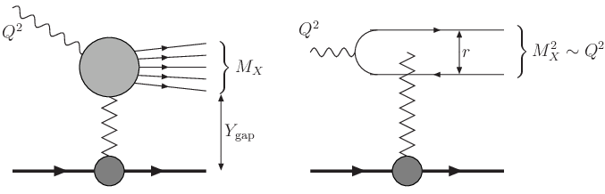
Returning to HERA physics, we shall conclude this review with a brief discussion of DIS diffraction, which is a particularly convenient laboratory to test saturation. Indeed, the diffractive cross–section is controlled by large dipole sizes and hence it is particularly sensitive to our theoretical ideas about unitarization. The theory is simpler for the case of a large rapidity gap , or small diffractive mass , in which case diffraction amounts to the elastic scattering of the dipole produced by the dissociation of (see Fig. 8). The respective cross–section is then evaluated as (compare to Eq. (1))
| (18) |
The photon wavefunction favors relatively small dipoles with :
| (19) |
But for small , , hence the integral will be dominated by the size where the amplitude has a turn–over, due to unitarity corrections. If unitarization is to be associated with the soft, non–perturbative, physics (the prevailing viewpoint before the advent of saturation; see, e.g., [65]), then , and diffraction would be non–perturbative even when is hard ! However, for sufficiently large (small ), the (semi)hard saturation scale enters the game and cuts off the integral in Eq. (19):
| (20) |
In this scenario, scales like the ‘hard Pomeron’, that is, in the same way as the inclusive cross–section (1); hence the ratio is approximately constant as a function of the energy. This prediction is to be contrasted to that of non–perturbative unitarization [65], where one rather expects the diffractive cross–section to rise twice as fast as the gluon distribution (since elastic scattering requires the exchange of at least two gluons), which would imply . It turns out that the HERA data favor the saturation scenario: the measured ratio is very flat as a function of the invariant energy , as illustrated in Fig. 9. This figure also shows that this flatness is well reproduced by the saturation model of Ref. [55]. Notice that the integrand in Eq. (20) rises as a double (hard) Pomeron, , but one power of is eventually compensated by the energy–dependence of the upper cutoff , which is the critical size for the onset of unitarity in the framework of saturation.

Acknowledgments
I would like to thank the organizers of the Ringberg Workshop “New Trends in HERA Physics 2008” for their warm hospitality at the Ringberg Castle. This work is supported in part by Agence Nationale de la Recherche via the programme ANR-06-BLAN-0285-01.
References
- [1] L.N. Lipatov, Sov. J. Nucl. Phys. 23 (1976) 338; E.A. Kuraev, L.N. Lipatov and V.S. Fadin, Zh. Eksp. Teor. Fiz 72, 3 (1977); Ya.Ya. Balitsky, L.N. Lipatov, Sov. J. Nucl. Phys. 28 (1978) 822.
- [2] L.V. Gribov, E.M. Levin, and M.G. Ryskin, Phys. Rept. 100 (1983) 1.
- [3] A.H. Mueller and J. Qiu, Nucl. Phys. B268 (1986) 427.
- [4] V.N. Gribov and L.N. Lipatov, Sov. Journ. Nucl. Phys. 15 (1972), 438; G. Altarelli and G. Parisi, Nucl. Phys. B126 (1977), 298; Yu. L. Dokshitzer, Sov. Phys. JETP 46 (1977), 641.
- [5] L. McLerran and R. Venugopalan, Phys. Rev. D49 (1994) 2233; ibid. 49 (1994) 3352; ibid. 50 (1994) 2225.
- [6] J. Jalilian-Marian, A. Kovner, A. Leonidov and H. Weigert, Nucl. Phys. B504 (1997) 415; Phys. Rev. D59 (1999) 014014; J. Jalilian-Marian, A. Kovner and H. Weigert, Phys. Rev. D59 (1999) 014015; A. Kovner, J. G. Milhano and H. Weigert, Phys. Rev. D62 (2000) 114005; H. Weigert, Nucl. Phys. A703 (2002) 823.
- [7] E. Iancu, A. Leonidov and L. McLerran, Nucl. Phys. A692 (2001) 583; Phys. Lett. B510 (2001) 133; E. Ferreiro, E. Iancu, A. Leonidov and L. McLerran, Nucl. Phys. A703 (2002) 489.
- [8] I. Balitsky, Nucl. Phys. B463 (1996) 99; Phys. Lett. B518 (2001) 235.
- [9] Yu.V. Kovchegov, Phys. Rev. D60 (1999) 034008; ibid. D61 (1999) 074018.
- [10] E. Iancu, A. Leonidov and L. McLerran, hep-ph/0202270; E. Iancu and R. Venugopalan, hep-ph/0303204; H. Weigert, hep-ph/0501087.
- [11] A. Stasto, K. Golec-Biernat and J. Kwiecinski, Phys. Rev. Lett. 86 (2001) 596.
- [12] C. Marquet and L. Schoeffel, Phys. Lett. B639 (2006) 471, hep-ph/0606079.
- [13] I. Arsene et al. [BRAHMS Collaboration], Phys. Rev. Lett. 93 (2004) 242303.
- [14] V.S. Fadin and L.N. Lipatov, Phys. Lett. B429 (1998) 127; G. Camici and M. Ciafaloni, Phys. Lett. B430 (1998) 349.
- [15] G.P. Salam, JHEP 9807 (1998) 19; M. Ciafaloni, D. Colferai, Phys. Lett. B452 (1999) 372; M. Ciafaloni, D. Colferai, and G.P. Salam, Phys. Rev. D60 (1999) 114036.
- [16] E. Iancu and L. McLerran, Phys. Lett. B510 (2001) 145.
- [17] A. H. Mueller, Nucl. Phys. B643 (2002) 501.
- [18] E. Iancu, K. Itakura, and L. McLerran, Nucl. Phys. A724 (2003) 181.
- [19] A. H. Mueller, Nucl. Phys. B558 (1999) 285.
- [20] Y. V. Kovchegov, J. Kuokkanen, K. Rummukainen and H. Weigert, arXiv:0812.3238
- [21] J. Jalilian-Marian and Y. V. Kovchegov, Prog. Part. Nucl. Phys. 56 (2006) 104.
- [22] F. Gelis, T. Lappi and R. Venugopalan, Int. J. Mod. Phys. E16 (2007) 2595.
- [23] M. Gyulassy, L. McLerran, Nucl. Phys. A750 (2005) 30; J.-P. Blaizot, F. Gelis, ibid. 148.
- [24] N. Armesto et al., J. Phys. G35 (2008) 054001 [arXiv:0711.0974 [hep-ph]].
- [25] Yu. V. Kovchegov and A. H. Mueller, Nucl. Phys. B529 (1998) 451; Yu. V. Kovchegov and K. Tuchin, Phys. Rev. D65 (2002) 074026.
- [26] C. Marquet, Nucl. Phys. B705 (2005) 319.
- [27] F. Gelis, T. Lappi and R. Venugopalan, arXiv:0804.2630; arXiv:0807.1306 [hep-ph].
- [28] I. Balitsky, Phys. Rev. D75 (2007) 014001; I. Balitsky and G. A. Chirilli, Phys. Rev. D77 (2008) 014019.
- [29] Y. V. Kovchegov and H. Weigert, Nucl. Phys. A784 (2007) 188; J. L. Albacete and Y. V. Kovchegov, Phys. Rev. D75 (2007) 125021.
- [30] A.H. Mueller, Nucl. Phys. A 724 (2003) 223.
- [31] E. Iancu, K. Itakura, and D.N. Triantafyllopoulos, Nucl. Phys. A742 (2004) 182.
- [32] E. Iancu and A.H. Mueller, Nucl. Phys. A730 (2004) 494.
- [33] A.H. Mueller and A.I. Shoshi, Nucl. Phys. B692 (2004) 175.
- [34] E. Iancu, A.H. Mueller and S. Munier, Phys. Lett. B606 (2005) 342.
- [35] E. Iancu and D.N. Triantafyllopoulos, Nucl. Phys. A756 (2005) 419; Phys. Lett. B610 (2005) 253.
- [36] A. Dumitru, E. Iancu, L. Portugal, G. Soyez and D. N. Triantafyllopoulos, JHEP 0708 (2007) 062.
- [37] E. Iancu, K. Itakura, and L. McLerran, Nucl. Phys. A708 (2002) 327.
- [38] A.H. Mueller and D.N. Triantafyllopoulos, Nucl. Phys. B640 (2002) 331.
- [39] S. Munier and R. Peschanski, Phys. Rev. Lett. 91 (2003) 232001.
- [40] For a review, see W. Van Saarloos, Phys. Rep. 386 (2003) 29.
- [41] D.N. Triantafyllopoulos, Nucl. Phys. B648 (2003) 293.
- [42] E. Iancu, K. Itakura and S. Munier, Phys. Lett. B590 (2004) 199.
- [43] G. Soyez, Phys. Lett. B655 (2007) 32.
- [44] A.H. Mueller, A.I. Shoshi, S.M.H. Wong, Nucl. Phys. B715 (2005) 440.
- [45] A. Kovner, M. Lublinsky, Phys. Rev. D71 (2005) 085004; Phys. Rev. Lett. 94 (2005) 181603.
- [46] Y. Hatta, E. Iancu, L. McLerran, A. Stasto, and D.N. Triantafyllopoulos, Nucl. Phys. A764 (2006) 423.
- [47] I. Balitsky, Phys. Rev. D72 (2005) 074027.
- [48] Y. Hatta, E. Iancu, C. Marquet, G. Soyez, and D.N. Triantafyllopoulos, Nucl. Phys. A773 (2006) 95.
- [49] E. Levin and M. Lublinsky, Nucl. Phys. A763 (2005) 172.
- [50] G. Soyez, Phys. Rev. D72 (2005) 016007.
- [51] R. Enberg, K. Golec–Biernat, and S. Munier, Phys. Rev. D72 (2005) 074021.
- [52] E. Iancu, J. T. de Santana Amaral, G. Soyez and D. N. Triantafyllopoulos, Nucl. Phys. A786 (2007) 131.
- [53] S. Munier, G. P. Salam and G. Soyez, arXiv:0807.2870 [hep-ph].
- [54] K. Golec-Biernat and M. Wüsthoff, Phys. Rev. D59 (1999) 014017; Phys. Rev. D60 (1999) 114023.
- [55] J. Bartels, K. Golec-Biernat, and H. Kowalski, Phys. Rev. D66 (2002) 014001.
- [56] H. Kowalski and D. Teaney, Phys. Rev. D68 (2003) 114005.
- [57] H. Kowalski, L. Motyka and G. Watt, Phys. Rev. D74 (2006) 074016.
- [58] G. Watt and H. Kowalski, Phys. Rev. D 78 (2008) 014016.
- [59] J. R. Forshaw, R. Sandapen and G. Shaw, Phys. Rev. D69 (2004) 094013; Phys. Lett. B594 (2004) 283.
- [60] J. R. Forshaw and G. Shaw, JHEP 0412, 052 (2004).
- [61] J. R. Forshaw, R. Sandapen and G. Shaw, JHEP 0611 (2006) 025.
- [62] D. Kharzeev, Y. V. Kovchegov and K. Tuchin, Phys. Lett. B599 (2004) 23.
- [63] A. Dumitru, A. Hayashigaki and J. Jalilian-Marian, Nucl. Phys. A A765 (2006) 464.
- [64] V. P. Goncalves, M. S. Kugeratski, M. V. T. Machado and F. S. Navarra, Phys. Lett. B643 (2006) 273.
- [65] J. D. Bjorken, arXiv:hep-ph/9601363.