This paper is a natural follow up to a previous work [1], where a new approach to the world sheet descripton of the planar graphs of the $\phi^{3}$ field theory was formulated. In contrast to the earlier work on the same subject [2,3,4,5], which used a first quantized formalism, the new formulation is based on second quantization on the world sheet. We have argued in [1] that this new formulation is both simpler and better founded than the old one. In the same reference, using a variational ansatz, an approximate ground state of the second quantized Hamiltonian was constructed in $5+1$ space-time dimensions. The ground state energy and the coupling constant turned out to be ultraviolet divergent, needing renormalization. Reassuringly, these divergences were the ones expected from the perturbation expansion of the underlying field theory.

In the present article, instead of the variational method, we use the mean field approximation for the same second quantized Hamiltonian. The motivation for doing this is twofold: We would like to check on the variational results, using a different approximation scheme. The mean field method has a long and honorable history in various branches of physics, and it was used in some of the early work [3,4,5] on this problem. It is reassuring that, as we shall see, using this alternate approach, we are able to confirm the results obtained in [1].

The second reason for trying a different approximation scheme is connected with the limitations of the variational method, which is useful only for investigating the ground state of a quantum system. For example, it is very difficult to extend its reach to the excited states. In contrast, using the mean field method, one can study the model in full generality, including the excited states. One of the main goals of this work is to show that with suitable tuning of the parameters of the model, there is string formation on the world sheet. We establish this result by showing that the spectrum of the excited states is that of a string.

As in the earlier work, a central role is played by the field $\rho$ defined on the world sheet by eq.(7). Roughly, $\rho$ measures the density of Feynman graphs on the world sheet, a concept which we will make more precise later on. An important question is whether $\rho_{0}$, the ground state expectation value of $\rho$, is different from zero. $\rho_{0}$ vanishes in any finite order of perturbation theory, whereas a non- zero value for $\rho_{0}$ means that the world sheet is densely covered by graphs, and the contribution of high (infinite) order graphs dominate. This can be thought of as a new phase of the underlying field theory, different from the perturbative phase. It is natural to expect that a world sheet densely covered by graphs would lead to a Nambu type action and hence result in string formation; in fact, this was the picture that motivated some of the very early work on this subject [6,7]. One of the main results of this paper is to show that the mean field calculation gives a non-zero $\rho_{0}$. We will show that such a non-trivial background exits as a solution to field equations, and furthermore it minimizes the ground state energy. This background will turn out to be an essential first step to showing string formation.

Along the way, we will study the ultraviolet divergences that are present in the expansion around the non-trivial background. These turn out the to be the ones expected from perturbation theory, and they can be renormalized. Of course, the divergences depend on the number of dimensions; in addition to $5+1$ dimensions, where the field theory is renormalizable and asymptotically free, we also consider $3+1$ dimensions, where the theory is superrenormalizable. The reason for this is that the superrenormalizable model with a fixed coupling constant is much easier to analyze, and provides a good warm up exercise for the more interesting but more difficult case of $5+1$ dimensions. We find it very encouraging that the mean field approximation simultaneously captures two desirable complimentary features: The ultraviolet behaviour is consistent with perturbation theory, and in the infrared region, the highly non-perturbative phenomenon of string formation takes place.

Let us summarize the main results to emerge from this investigation. Applying the mean field approximation to the world world sheet field theory developed in [1], we have found a non-trivial solution to field equations, with $\rho_{0}\neq 0$, which minimizes the ground state energy. This background is in agreement with the variational wave function derived in [1]. It also means that the phase where the world sheet is densely covered by graphs is energetically prefered. Expanding around this background to second order, and with some tuning the parameters of the model, we find that the spectrum of the model is that of a bosonic string.

In order to have a self contained paper, in sections 2 and 3, we review briefly the background needed to understand the present work. In section 2, we discuss the general setup on the world sheet [2,8], and in section 3, we review the world sheet field theory developed in [1]. In section 4, we develop the mean field approximation and set up the corresponding mean field equations. In section 5, these equations are used to find the ground state of the model in both $3+1$ and $5+1$ dimensions. Along the way, we encounter ultraviolet divergences and show how to eliminate them by renormalization. In particular, in $5+1$ dimensions, the cutoff dependence of the bare coupling constant is consistent with asymptotic freedom. In section 6, we expand the Hamiltonian to second order around the background found in the previous section. The solution to the resulting equations yields two different types of spectra: bound states at lower energies and a continuum starting at a higher energy. In section 7, we show that the spectrum of the bound states is that of a string with linear trajectories; however, the higher excited states of the string mix with the continuum, which muddies the string picture. It turns out that, by a suitable adjustment of the parameters of the model, one can push the continuum arbitrarily high, and thereby extend the string picture to arbitrarily high energies. Finally, in section 8, we summarize our conclusions and suggest some directions for future research.

The generic planar graphs of the $\phi^{3}$ in the mixed light cone representation of ’t Hooft [8] have a particularly simple form. The world sheet is parametrized by the two coordinates

$$\tau=x^{+}=(x^{0}+x^{1})/\sqrt{2},\,\,\sigma=p^{+}=(p^{0}+p^{1})/\sqrt{2}.$$

A general planar graph is represented by a collection of horizontal solid lines (Fig.1), where the n’th solid line carries a $D$ dimensional transverse momentum ${\bf q}_{n}$.

Two adjacent solid lines labeled by n and n+1 correspond to the light cone propagator

$$\Delta(p_{n})=\frac{\theta(\tau)}{2p^{+}}\,\exp\left(-i\tau\,\frac{{\bf p}_{n}^{2}+m^{2}}{2p^{+}}\right),$$

(1)

where ${\bf p}_{n}={\bf q}_{n}-{\bf q}_{n+1}$. A factor of $g$, the coupling constant, is inserted at the beginning and at the end of each line, where the interaction takes place.

For technical reasons, it is convenient to discretize the coordinate $\sigma$ in steps of length $a$, which amounts to compactifying the light cone coordinate $x^{-}=(x^{0}-x^{1})/\sqrt{2}$ at radius $R=1/a$. This type of compactification was introduced by Casher [9] in the context of the lightcone quantization of gauge theories. In the context of the lightcone worldsheet and the discretization of the $\sigma$ coordinate to enable summing planar diagrams, this discretization was first proposed and exploited by Giles and Thorn [10]. Later, it was found useful in connection with the M theory [11,12]. In this paper, the $\sigma$ coordinate will always be discretized; in contrast, the time coordinate $\tau$ will remain continuous.

We also have to specify the boundary conditions to be imposed on the world sheet. For simplicity, the coordinate $\sigma$ is compactified by imposing periodic boundary conditions at $\sigma=0$ and $\sigma=p^{+}$, where $p^{+}$ is the total $+$ component of the momentum flowing through the whole graph. In contrast, since we will adopt the Hamiltonian approach, the boundary conditions at $\tau=\pm\infty$ will be left free.

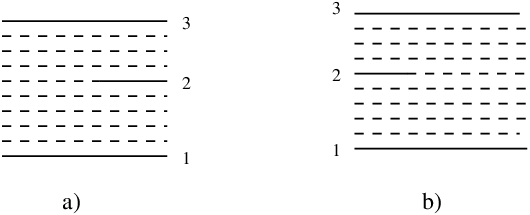
There is a useful way of visualizing the discretized world sheet. As pictured in Fig.2, the world sheet consists of horizontal dotted and solid lines, spaced a distance $a$ apart.

Just as in Fig.1, the boundaries of the propagators are marked by solid lines, in contrast, the bulk is filled with dotted lines. Ultimately, one has to integrate over all possible locations and lengths of solid lines, as well as over the transverse momenta they carry.

In this section, we will briefly review the world sheet field theory developed in [1], which reproduces the light cone graphs described in the previous section. We start by introducing the bosonic field $\phi(\sigma,\tau,{\bf q})$, and its conjugate $\phi^{\dagger}(\sigma,\tau,{\bf q})$, which at time $\tau$ respectively annihilate and create a solid line carrying momentum ${\bf q}$ and located at site labeled by $\sigma$. They satisfy the commutation relations

$$[\phi(\sigma,\tau,{\bf q}),\phi^{\dagger}(\sigma^{\prime},\tau^{\prime},{\bf q^{\prime}})]=\delta_{\sigma,\sigma^{\prime}}\,\delta({\bf q}-{\bf q^{\prime}}).$$

(2)

The vacuum corresponds to a state with only dotted lines (empty world sheet), and it satisfies

$$\phi(\sigma,{\bf q})|0\rangle=0.$$

(3)

Since we are in the Hamiltonian picture with time $\tau$ is fixed, in equations of this type, we do not usually explicitly write the time dependence. By applying $\phi^{\dagger}$ s on vacuum, one can then construct states with arbitrary number of solid lines.

Having defined the Fock space, a first go at the Hamiltonian could look like the following:

	$\displaystyle H$	$\displaystyle=$	$\displaystyle H_{0}+H_{I},$
	$\displaystyle H_{0}$	$\displaystyle=$	$\displaystyle\sum_{\sigma^{\prime}>\sigma}\int d{\bf q}\int d{\bf q^{\prime}}\frac{({\bf q}-{\bf q^{\prime}})^{2}+m^{2}}{2(\sigma^{\prime}-\sigma)}\phi^{\dagger}(\sigma,{\bf q})\,\phi(\sigma,{\bf q})\,\phi^{\dagger}(\sigma^{\prime},{\bf q^{\prime}})\,\phi(\sigma^{\prime},{\bf q^{\prime}}),$
	$\displaystyle H_{I}$	$\displaystyle=$	$\displaystyle g\sum_{\sigma}\int d{\bf q}\left(\phi(\sigma,{\bf q})+\phi^{\dagger}(\sigma,{\bf q})\right).$		(4)

It is easy to check that $H_{0}$, applied to a state with two solid lines, generates the free propagator of eq.(1), and $H_{I}$, converting a solid line into a dotted one and vice versa, generates the interaction. There are, however, several problems with this guess for the Hamiltonian:
a) The Hilbert space has redundant states, corresponding to multiple solid lines at the same site, generated by repeated applications of $\phi^{\dagger}$ at the same $\sigma$.
b) Propagators should be assigned only to adjacent solid lines, whereas the above $H_{0}$ generates unallowed propagators associated with non-adjacent solid lines.
c) The prefactor $1/(2p^{+})$ of the propagator is missing.

These problems can be solved simultaneously by introducing a two component fermion field $\psi_{i}(\sigma,\tau)$, $i=1,2$, and its adjoint $\bar{\psi}_{i}$ on the world sheet [13]. They satisfy the standard anticommutation relations

$$[\psi_{i}(\sigma,\tau),\bar{\psi}_{i^{\prime}}(\sigma^{\prime},\tau)]_{+}=\delta_{i,i^{\prime}}\delta_{\sigma,\sigma^{\prime}},$$

(5)

and propagate freely on an uninterrupted line. The fermion with $i=1$ lives on the dotted lines and the one with $i=2$ lives on the solid lines. It was shown in [1] how to overcome the problems listed above with the help of the fermions. Here, we will only present the final result, and refer the reader to [1] for the details.

To get rid of the redundant states, we impose the following constraint at a fixed time on the Fock space:

$$\int d{\bf q}\,\phi^{\dagger}(\sigma,{\bf q})\phi(\sigma,{\bf q})-\rho(\sigma)=0,$$

(6)

where $\rho$ is the composite field

$$\rho=\frac{1}{2}\bar{\psi}(1-\sigma_{3})\psi,$$

(7)

which is equal to one on solid lines and zero on the dotted lines. This constraint ensures that there is at most one solid line at each site, thereby avoiding problem a).

To avoid the unwanted propagators of b), we define, for any two lines located at $\sigma_{i}$ and $\sigma_{j}$, with $\sigma_{j}>\sigma_{i}$,

$$\mathcal{E}(\sigma_{i},\sigma_{j})=\prod_{k=i+1}^{k=j-1}\left(1-\rho(\sigma_{k})\right).$$

(8)

If $\sigma_{j}<\sigma_{i}$, $\mathcal{E}$ is defined to be zero. The following property of this function that will be needed: $\mathcal{E}(\sigma_{i},\sigma_{j})$ is equal to one only if the two solid lines at $\sigma_{i}$ and $\sigma_{j}$ are seperated only by dotted lines. If there is one or more solid lines in between, it is zero. If we now redefine $H_{0}$ as

	$\displaystyle H_{0}$	$\displaystyle=$	$\displaystyle\frac{1}{2}\sum_{\sigma,\sigma^{\prime}}\int d{\bf q}\int d{\bf q^{\prime}}\,\frac{\mathcal{E}(\sigma,\sigma^{\prime})}{\sigma^{\prime}-\sigma}\left(({\bf q}-{\bf q^{\prime}})^{2}+m^{2}\right)$		(9)
		$\displaystyle\times$	$\displaystyle\phi^{\dagger}(\sigma,{\bf q})\,\phi(\sigma,{\bf q})\,\phi^{\dagger}(\sigma^{\prime},{\bf q^{\prime}})\,\phi(\sigma^{\prime},{\bf q}).$

By applying $H_{0}$ to a state with several solid lines, it is easy to see that $\mathcal{E}(\sigma,\sigma^{\prime})$ projects out all the unwanted propagators.

There remains the problem c), the problem of the missing prefactor. As explained in reference [1], it is best to attach this factor to the vertices. Consider two types of vertices, corresponding to the beginning and ending of a solid line, pictured in Fig.3.

The solid lines are labeled as 1, 2 and 3, and the momenta that enter the vertices are labeled by the corresponding pair of indices 12, 23 and 13 respectively. Attaching a factor of

$$V=\frac{1}{\sqrt{8\,p_{12}^{+}p_{23}^{+}p_{13}^{+}}}=\frac{1}{\sqrt{8(\sigma_{2}-\sigma_{1})(\sigma_{3}-\sigma_{2})(\sigma_{3}-\sigma_{1})}}$$

(10)

to each vertex, takes care of the missing prefactors. However, we still face a problem similar to the one encountered with the construction of $H_{0}$. In the vertices of Fig.3 , the solid lines 1 and 3 at one end of the vertex should be seperated by only the dotted lines. To ensure this, we define

$$\mathcal{V}(\sigma_{2})=\sum_{\sigma_{1}<\sigma_{2}}\sum_{\sigma_{2}<\sigma_{3}}\frac{\rho(\sigma_{1})\mathcal{E}(\sigma_{1},\sigma_{3})\rho(\sigma_{3})}{\sqrt{8(\sigma_{2}-\sigma_{1})(\sigma_{3}-\sigma_{2})(\sigma_{3}-\sigma_{1})}}.$$

(11)

The numerator of this expression picks the correct vertex configuration, and it projects out all the other unwanted configurations. With the help of this vertex, we can rewrite the final form of $H_{I}$, which includes the additional factor $V$ of eq.(10):

$$H_{I}=g\sum_{\sigma}\int d{\bf q}\left(\mathcal{V}(\sigma)\,\phi(\sigma,{\bf q})\,\rho_{+}(\sigma)+\rho_{-}(\sigma)\,\phi^{\dagger}(\sigma,{\bf q})\,\mathcal{V}(\sigma)\right),$$

(12)

where,

$$\rho_{\pm}=\frac{1}{2}\bar{\psi}(\sigma_{1}\pm i\sigma_{2})\psi.$$

The additional factors $\rho_{\pm}$ are needed to make sure that a solid line in the Fock space is always paired with an $i=2$ fermion and a dotted line with an $i=1$ fermion.

Now that the various pieces that make up the total Hamiltonian are in place, we define,

$$H=H_{0}+H_{I}+H^{\prime},$$

(13)

where $H_{0}$ and $H_{I}$ are given by eqs.(9) and (12), and,

$$H^{\prime}=\sum_{\sigma}\left(\int d{\bf q}\,\phi^{\dagger}(\sigma,{\bf q})\,\phi(\sigma,{\bf q})-\rho(\sigma)\right)\,\lambda(\sigma),$$

(14)

implements the constraints (6) by means of a Lagrange multiplier $\lambda$.

Taking advantage of (6), it is possible to rewrite the free Hamiltonian in a somewhat simpler form:

	$\displaystyle H_{0}$	$\displaystyle=$	$\displaystyle\frac{1}{2}\sum_{\sigma\neq\sigma^{\prime}}G(\sigma,\sigma^{\prime})\Big(\rho(\sigma)\,\int d{\bf q^{\prime}}\,{\bf q^{\prime}}^{2}\,\phi^{\dagger}(\sigma^{\prime},{\bf q^{\prime}})\,\phi(\sigma^{\prime},{\bf q^{\prime}})+\frac{1}{2}m^{2}\rho(\sigma)\rho(\sigma^{\prime})$		(15)
		$\displaystyle-$	$\displaystyle\int d{\bf q}\int d{\bf q^{\prime}}\,({\bf q}\cdot{\bf q^{\prime}})\,\phi^{\dagger}(\sigma,{\bf q})\,\phi(\sigma,{\bf q})\,\phi^{\dagger}(\sigma^{\prime},{\bf q^{\prime}})\,\phi(\sigma^{\prime},{\bf q^{\prime}})\Big),$

where, to simplify writing, we have defined,

$$G(\sigma,\sigma^{\prime})=\frac{\mathcal{E}(\sigma,\sigma^{\prime})+\mathcal{E}(\sigma^{\prime},\sigma)}{|\sigma-\sigma^{\prime}|}.$$

Although we will mostly stick with the Hamiltonian picture in this paper, if so desired, one can switch to the path integral approach based on the action

$$S=\int d\tau\left(\sum_{\sigma}\left(i\bar{\psi}\partial_{\tau}\psi+i\int d{\bf q}\,\phi^{\dagger}\partial_{\tau}\phi\right)-H(\tau)\right).$$

(16)

It is easy to verify that the above action is invariant under the following phase transformation:

	$\displaystyle\psi$	$\displaystyle\rightarrow$	$\displaystyle\exp\left(-\frac{i}{2}\,\alpha\,\sigma_{3}\right)\,\psi,\,\,\,\bar{\psi}\rightarrow\bar{\psi}\,\exp\left(\frac{i}{2}\,\alpha\,\sigma_{3}\right),$
	$\displaystyle\phi$	$\displaystyle\rightarrow$	$\displaystyle\exp(-i\,\alpha\,)\,\phi,\,\,\,\phi^{\dagger}\rightarrow\exp(i\,\alpha\,)\,\phi^{\dagger},\,\,\,\lambda\rightarrow\lambda-\partial_{\tau}\alpha.$		(17)

Here $\alpha$ is an arbitrary function of $\sigma$ and $\tau$, so this is a gauge transformation on the world sheet. By a suitable gauge fixing, it should be possible to eliminate one of the degrees of freedom of the fermionic field $\psi$. To see how this comes about, it is very convenient first to bosonize $\psi$. In addition to $\rho$ (eq.(7)), we introduce the bosonic field $\xi$ and set,

	$\displaystyle\bar{\psi}\sigma_{3}\psi$	$\displaystyle=$	$\displaystyle 1-2\,\rho,\,\,\,\bar{\psi}\sigma_{1}\psi=2\,\sqrt{\rho-\rho^{2}}\,\cos(\xi),$
	$\displaystyle\bar{\psi}\sigma_{2}\psi$	$\displaystyle=$	$\displaystyle 2\,\sqrt{\rho-\rho^{2}}\,\sin(\xi).$		(18)

The first equation is simply a rewrite of eq.(7). The kinetic energy term for $\psi$ in eq.(16) can be replaced by its bosonic counterpart:

$$\int d\tau\sum_{\sigma}i\,\bar{\psi}\partial_{\tau}\psi\rightarrow\int d\tau\sum_{\sigma}\xi\,\partial_{\tau}\rho.$$

(19)

One can check that this action produces the correct equations of motion and the correct commutation relations for the fermionic bilinears.

We note that bosonization has replaced discrete variables by continous ones. For example, according to its original definition as a composite field (eq.(7)), $\rho$ could only take on the values 0 and 1, but as an independent bosonic field, it can vary continuously between 0 and 1. It is natural to interpret it as the probability of finding a solid line at a given location. As we shall see in the next section, the reformulation of the problem in terms of continuous variables provides a convenient setup for the mean field approximation.

Now consider the effect of the phase transformation (17) on the bosonic fields: $\rho$ is unchanged, whereas $\xi$ transforms according to

$$\xi\rightarrow\xi+\alpha,$$

and therefore, we can gauge fix by setting

$$\xi=0.$$

(20)

In this gauge, and with fermions bosonized, the interaction Hamiltonian (12) becomes

$$H_{I}\rightarrow g\,\sum_{\sigma}\,\mathcal{V}(\sigma)\,\sqrt{\rho(\sigma)-\rho^{2}(\sigma)}\,\int d{\bf q}\,\left(\phi(\sigma,{\bf q})+\phi^{\dagger}(\sigma,{\bf q})\right).$$

(21)

Although the field $\xi$ disappeared from the problem, its equation of motion, namely

$$\partial_{\tau}\rho=0,$$

(22)

has to be imposed as a constraint. This constraint means that being time independent, $\rho$ is no longer a dynamical field. Recalling that we have not specified the initial conditions, we can do so now by assigning an arbitrary probability distribution $\rho(\sigma)$ for the solid lines at some initial time. This probability distribution is then constant in time by virtue of the above constraint. In the next section, $\rho(\sigma)$ will be determined in the mean field approximation by minimizing the ground state energy.

The Hamiltonian (13) is exact but quite complicated; for example, it is non-local in the coordinate $\sigma$. Clearly, it is not a good starting point for doing the usual Feynman perturbation expansion. The standard perturbation theory is an expansion in the $\rho_{0}=0$ phase of the model. Instead, we are here interested in the phase where Feynman graphs are dense on the world sheet, with $\rho_{0}\neq 0$. In this new phase, the Hamiltonian (13), in conjunction with the mean field method, turns out to be an excellent starting point for doing calculations. In fact, in the standard approach, one would be at a loss to even define the new phase precisely.

In reference [1], a variational approach was used to calculate the ground state of (13). Here, instead, the mean field approximation will enable us to compute, in addition to the ground state, the excited modes of the model. We should point out right at the beginning that, for the meanfield method to make sense, we have to take the total number of lines on the world sheet,

$$N_{0}=p^{+}/a,$$

(23)

to be large but finite. So we are close to the world sheet continuum limit, but $a$ is always kept non-zero to avoid ill defined expressions.

The mean field approximation amounts to replacing every bosonic field in the Hamiltonian by its ground state expectation value, and then minimizing the resulting ground state energy. The subscript “0” will indicate the expectation value of the corresponding field; for example, $\langle\rho\rangle=\rho_{0},\,\langle\phi\rangle=\phi_{0}$, and so on. We will assume that the ground state is invariant under translations of $\sigma$ and $\tau$, so that the expectation values of the fields do not depend on these variables. Therefore, $\rho_{0}$ and $\lambda_{0}$ are constants, whereas $\phi_{0}$ and $\phi^{\dagger}_{0}$ depend only on ${\bf q}$. Furthermore, by rotation invariance, they can only depend on the length of the vector ${\bf q}$. We also note that in view of the discussion at the end of the last section, $\rho$ is not a dynamical field but it merely serves to fix the initial conditions. Letting $\rho\rightarrow\rho_{0}$ is an exact replacement; there are no fluctuations around $\rho_{0}$. This means that we have once for all fixed the initial conditions so as to minimize the ground state energy.

Replacing every bosonic field by its expectation value, as indicated above, considerably simplifies the Hamiltonian. Let us start with the free Hamiltonian $H_{0}$. Setting $\rho=\rho_{0}$ in the definition of $\mathcal{E}$, we have,

	$\displaystyle\mathcal{E}(\sigma,\sigma^{\prime})$	$\displaystyle=$	$\displaystyle(1-\rho_{0})^{n},\,\,\,n=(\sigma^{\prime}-\sigma)/a-1,$
	$\displaystyle G(\sigma,\sigma^{\prime})$	$\displaystyle=$	$\displaystyle\frac{(1-\rho_{0})^{n}}{a(n+1)},\,\,\,\sigma^{\prime}>\sigma,$
	$\displaystyle\sum_{\sigma^{\prime}>\sigma}G(\sigma,\sigma^{\prime})$	$\displaystyle=$	$\displaystyle-\frac{\ln(\rho_{0})}{a(1-\rho_{0})}.$		(24)

In writing this equation, we have assumed that the sum over $n$ extends all the way to infinity, whereas in reality, there is an upper cutoff of the order of $N_{0}$ (eq.(23)). But since $N_{0}$ is very large, this makes a difference only for very small values of $\rho_{0}$. In what follows, we will always keep $\rho_{0}$ away from zero. Substituting the above result in $H_{0}$, we get,

$$E_{0}=\langle H_{0}\rangle=N_{0}F(\rho_{0})\left(\int d{\bf q}\,{\bf q}^{2}\,|\phi_{0}({\bf q})|^{2}+\frac{1}{2}m^{2}\,\rho_{0}\right),$$

(25)

where we have defined,

$$F(\rho_{0})=-\frac{\rho_{0}\,\ln(\rho_{0})}{a(1-\rho_{0})}.$$

Notice that the last term on the right hand side of eq.(15) vanishes because of the rotation invariance of $\phi_{0}({\bf q})$.

Next, we focus on $H_{I}$ (eq.(21)), replacing $\rho$ by $\rho_{0}$ and $\phi$ by $\phi_{0}$.ith this replacement, $\mathcal{V}$ becomes independent of $\sigma_{2}$; it depends implicitly only on $\rho_{0}$:

	$\displaystyle\mathcal{V}$	$\displaystyle=$	$\displaystyle\frac{\rho_{0}^{2}}{\sqrt{8a^{3}}}\,W(\rho_{0}),$
	$\displaystyle W(\rho_{0})$	$\displaystyle=$	$\displaystyle\sum_{n_{1}=0}^{\infty}\sum_{n_{2}=0}^{\infty}\frac{(1-\rho_{0})^{n_{1}+n_{2}+1}}{\sqrt{(n_{1}+1)(n_{2}+1)(n_{1}+n_{2}+2)}}.$		(26)

The ground state value of $H_{I}$, $E_{I}$, is then given by

$$E_{I}=N_{0}\,g\,\mathcal{V}(\rho_{0})\,\sqrt{\rho_{0}-\rho_{0}^{2}}\,\int d{\bf q}\,\left(\phi_{0}({\bf q})+\phi_{0}^{*}({\bf q})\right),$$

(27)

and the total ground state energy $E_{t}$ by

$$E_{t}=E_{0}+E_{I}+N_{0}\,\lambda_{0}\,\left(\int d{\bf q}\,|\phi_{0}({\bf q})|^{2}-\rho_{0}\right),$$

(28)

where $E_{0}$ is given by (25).

The next step is to write down the classical equations of motion that result from varying $E_{t}$ with respect to the expectation values of the fields. The solution to these equations will then determine the ground state energy. We will first write down the equations gotten by varying $E_{t}$ with respect to $\phi_{0}$ and $\lambda_{0}$:

	$\displaystyle\frac{\partial E_{t}}{\partial\phi_{0}({\bf q})}=0$	$\displaystyle\rightarrow$	$\displaystyle\phi_{0}=\phi_{0}^{*}=-g\,\frac{\sqrt{\rho_{0}-\rho_{0}^{2}}\,\mathcal{V}(\rho_{0})}{\lambda_{0}+F(\rho_{0})\,{\bf q}^{2}},$		(29)
	$\displaystyle\frac{\partial E_{t}}{\partial\lambda_{0}}=0$	$\displaystyle\rightarrow$	$\displaystyle\rho_{0}=g^{2}\,\mathcal{V}^{2}(\rho_{0})\,(\rho_{0}-\rho_{0}^{2})\,\int d{\bf q}\,\left(\lambda_{0}+F(\rho_{0})\,{\bf q}^{2}\right)^{-2}.$		(30)

Apart from some redefinition of constants, $\phi_{0}({\bf q})$ is the same as the variational wave function $A({\bf q})$ of reference [1]. This suggests that the mean field and the variational approximations are closely related.

Our goal is to eliminate all subsidiary variables except for $\rho_{0}$, and to express $E_{t}$ in terms of only this remaining variable. We will then search for the minimum value of $E_{t}$ and see whether this is realized for a value of $\rho_{0}$ different from zero and one. As explained earlier, if $\rho_{0}$ turns out to be zero, we then have a trivial ground state corresponding to an empty world sheet. $\rho_{0}=1$ corresponds to a world sheet where every line is an eternal solid line, which is simply a bunch of free propagators and therefore trivial. In contrast, a value for $\rho_{0}$ different from zero or unity means that the ground state corresponds to a world sheet densely covered by interacting Feynman graphs. This is the kind of ground state that can lead to interesting phenomena, such as string formation.

Equation (30) involves an integral over ${\bf q}$, and in order to proceed further, the dimension $D$ of the transverse space, which has been arbitrary up to now, has to be specified. We will investigate this equation for $D=2$ and $D=4$ in the next section.

$D=2$ (3+1 space-time dimensions) and $D=4$ (5+1 space-time dimensions) are two interesting choices for the $\phi^{3}$ theory. In the first case, the model is superrenormalizable; the coupling constant is finite, and there is only a logarithmic mass divergence. Eqs. (29) and (30) can be used to eliminate $\lambda_{0}$ and $\phi_{0}$, and therefore the ground state energy $E_{t}$ can be expressed solely in terms of $\rho_{0}$. In contrast, at $D=4$, the model is renormalizable and asymptotically free. In this case, $\lambda_{0}$ stays in the problem and it can be used to define the renormalized coupling constant through eq.(38). This is a familiar situation, related to asymptotic freedom and the running of the coupling constant. All of this is in complete agreement with the well known results from perturbation theory.

Let us now set $D=2$ in eq.(30). The integral is finite, and after doing it, the result can be written as

$$\lambda_{0}=\pi\,g^{2}\,\mathcal{V}^{2}(\rho_{0})\,\frac{1-\rho_{0}}{F(\rho_{0})}.$$

(31)

Combining this with (29), $E_{t}$ can be expressed as a function of only $\rho_{0}$. The result, however, contains two integrals

$$\int d{\bf q}\,\phi_{0}({\bf q}),\,\,\,\int d{\bf q}\,{\bf q}^{2}\,\phi_{0}^{2}({\bf q}),$$

which diverge logarithmically for large ${\bf q}$. We evaluate these using a cutoff $\Lambda$ in $|{\bf q}|$, and obtain the following final result for the ground state energy:

$$E_{t}=N_{0}\left(-\pi\,g^{2}\,\mathcal{V}^{2}(\rho_{0})\,\frac{\rho_{0}-\rho_{0}^{2}}{F(\rho_{0})}\left(\ln\left(\frac{F\,\Lambda^{2}}{\lambda_{0}}\right)+1\right)+\frac{1}{2}\,m^{2}\,\rho_{0}\,F(\rho_{0})\right).$$

(32)

To minimize the energy, we search for the solutions of

$$\frac{\partial E_{t}}{\partial\rho_{0}}=0.$$

(33)

We note that, in the limit $\Lambda\rightarrow\infty$, the location of the minimum is solely determined by the cutoff dependent term in $E_{t}$. At the same time, we would like to introduce a mass counter term to cancel the cutoff dependence. This is done by replacing $m$ in (25) by the bare mass $m_{0}$ and setting

$$m_{0}^{2}=s\,\ln\left(\Lambda^{2}/\mu^{2}\right),$$

(34)

where $s$ is a parameter which will later be ajusted to cancel the divergence. One has first to minimize the cutoff dependent terms in $E_{t}$ at fixed $s$ and $\Lambda$ with respect to $\rho_{0}$, and then adjust $s$ so that in the final expression, the logarithmic divergence cancels. This leads to two simultaneous equations for the two parameters $\rho_{0}$ and $s$:

	$\displaystyle-\pi\,g^{2}\,\frac{\partial}{\partial\rho_{0}}\left(\mathcal{V}^{2}(\rho_{0})\,\frac{\rho_{0}-\rho_{0}^{2}}{F(\rho_{0})}\right)+\frac{1}{2}\,s\,\frac{\partial}{\partial\rho_{0}}\left(\rho_{0}\,F(\rho_{0})\right)=0,$
	$\displaystyle-\pi\,g^{2}\,\mathcal{V}^{2}(\rho_{0})\,\frac{(\rho_{0}-\rho_{0}^{2})}{F(\rho_{0})}+\frac{1}{2}\,s\,\rho_{0}\,F(\rho_{0})=0.$		(35)

Eliminating $s$, the two equations reduce to a single equation:

$$\frac{\partial L(\rho_{0})}{\partial\rho_{0}}=0,$$

(36)

where $L$ is given by

$$L(\rho_{0})=\frac{W^{2}(\rho_{0})\,\rho_{0}^{2}\,(1-\rho_{0})^{3}}{\ln^{2}(\rho_{0})},$$

and $W$ by (26). Now,

$$W(\rho_{0})\rightarrow\pi^{3/2}\,(\rho_{0})^{-1/2}$$

as $\rho_{0}\rightarrow 0$, and

$$W(\rho_{0})\rightarrow 2^{-1/2}\,(1-\rho_{0})$$

as $\rho_{0}\rightarrow 1$. The function $L$, schematically plotted as a function of $x=\rho_{0}$ in Fig.(4),

vanishes at both $\rho_{0}=0$ and $\rho_{0}=1$, and it is positive in between. Its derivative has a single zero in the interval, corresponding to cutoff independent minimum for $E_{t}$ at $\rho_{0}\neq 0$. The coefficient of the logarithmic cutoff term in $E_{t}$,

$$Z(\rho_{0})=-\pi\,g^{2}\,\mathcal{V}^{2}(\rho_{0})\,\frac{\rho_{0}-\rho_{0}^{2}}{F(\rho_{0})}+\frac{1}{2}\,s\,\rho_{0}\,F(\rho_{0}),$$

(37)

is plotted schematically as a function of $x=\rho_{0}$ in Fig.(5).

There are two minima, a trivial one at $\rho_{0}=0$, and the non-trivial one at some point in the interval $0<\rho_{0}<1$. Although these minima appear degenerate, that is because $Z$ does not include the cutoff independent terms in $E_{t}$. These terms have no influence on the position of the minima, but the value of $E_{t}$ at the non-trivial minimum does depend on them. For example, we can change it by adding an arbitrary cutoff independent term to $m_{0}^{2}$ in (30). In this way, we can adjust $E_{t}$ to be negative at the non-trivial minimum, so that it becomes the true global minimum. We conclude that one can arrange to have a global minimum of the energy which is cutoff independent at a non-zero value of $\rho_{0}$.

Let us now consider the case $D=4$. The integral that appears in equation (30) is now logarithmically divergent. We introduce a cutoff $\Lambda$ as before, and after doing the integral, the result can be written in the form,

$$\frac{1}{g_{0}^{2}}=\pi^{2}\,\mathcal{V}^{2}(\rho_{0})\,\frac{1-\rho_{0}}{F^{2}(\rho_{0})}\,\left(\ln\left(\frac{\rho_{0}\,F\,\Lambda^{2}}{\lambda_{0}}\right)-1\right),$$

(38)

where $g$ has been replaced by $g_{0}$ in anticipation of renormalization. It is now natural to define the renormalized coupling constant $g_{r}$ at the energy scale corresponding to $\lambda_{0}$: by

$$g_{r}^{2}=g_{0}^{2}\,\ln\left(\frac{\Lambda^{2}}{\lambda_{0}}\right).$$

(39)

This equation is consistent with the well known asymptotic freedom of the $\phi^{3}$ theory in $5+1$ dimensions. Also, the results derived here, using the mean field method, in particular the expression for $\phi_{0}$ (eq.(29)), are in agreement with those derived in [1] using a variational calculation.

Just as in the case $D=2$, the ground state energy $E_{t}$ can be calculated by eliminating the auxilliary variables. The integrals over ${\bf q}$ that one encounters are now quadratically divergent, and the leading cutoff dependent piece plus the mass term in $E_{t}$ is given by

$$E_{t}\approx N_{0}\,\left(-\pi^{2}\,g^{2}\,\mathcal{V}^{2}(\rho_{0})\,\frac{\rho_{0}-\rho_{0}^{2}}{F(\rho_{0})}\,\Lambda^{2}+\frac{1}{2}\,m_{0}^{2}\,\rho_{0}\,F(\rho_{0})\right).$$

(40)

Apart from a different power of $\pi$, the coefficient of $\Lambda^{2}$ is identical to the coefficient of $\ln(\Lambda)$ in (32) for $D=2$. Consequently, letting

$$m_{0}^{2}=s\,\Lambda^{2},$$

we end up with eq. (36), and the same minimum $\rho_{0}\neq 0$ as before.

In the last section, using the mean field approximation, we found a non-trivial ground state corresponding to non-vanishing bosonic fields. The next step would be to treat this solution as a classical background, and to calculate the quadratic fluctuations about this background. This would then give us the spectrum of the free theory based on this new ground state. The cubic and higher order terms in the fluctuations will be responsible for the interactions and they will not be considered here. We will see in this section that, the spectrum of the fluctuating modes consists of two sectors: A continuum and discrete bound states. It is the bound states that generate the string spectrum, which eventually merges into the continuum. In an appropriately defined limit $N_{0}\rightarrow\infty$, the continuum can be pushed all the way up, leaving behind the spectrum of a free bosonic string. As discussed in the introduction, this is not unexpected: When the world sheet is uniformly and densely covered by graphs, it is reasonable to expect that it can be described by an effective Nambu action, leading to a string picture.

In what follows, we will fix the fields $\lambda$ and $\rho$ at their classical values $\lambda_{0}$ and $\rho_{0}$ respectively. For the field $\rho$, this is no restriction; as we have argued earlier, $\rho$ is fixed by the boundary conditions and does not fluctuate. $\lambda$ could in principle fluctuate; however, since this field carries no momentum, it is not expected to contribute to the string trajectories. The only fields that carry momentum are $\phi(\sigma,{\bf q})$ and $\phi^{\dagger}(\sigma,{\bf q})$, and we will calculate to second order the fluctuations of these fields around their ground state expectation values.

Defining $H_{p}$ the collection of $\phi$ dependent terms in the Hamiltonian, we have,

	$\displaystyle H_{p}$	$\displaystyle=$	$\displaystyle\sum_{\sigma,\sigma^{\prime}}\,\frac{1}{2}\,G(\sigma,\sigma^{\prime})\,\Big(\rho_{0}\,\int d{\bf q}\,{\bf q}^{2}\,\phi^{\dagger}(\sigma,{\bf q})\,\phi(\sigma,{\bf q})+\lambda_{0}\,\int d{\bf q}\,\phi^{\dagger}(\sigma,{\bf q})\,\phi(\sigma,{\bf q})$		(41)
		$\displaystyle-$	$\displaystyle\int d{\bf q}\,\int d{\bf q^{\prime}}\,({\bf q}\cdot{\bf q^{\prime}})\phi^{\dagger}(\sigma,{\bf q})\,\phi(\sigma,{\bf q})\,\phi^{\dagger}(\sigma^{\prime},{\bf q^{\prime}})\,\phi(\sigma^{\prime},{\bf q^{\prime}})\Big).$

We have not included $H_{I}$ since it is linear in $\phi$ and $\phi^{\dagger}$ and consequently does not contribute to the quadratic terms in fluctuations. Before expanding $H_{p}$ around the classical background, it is convenient to define

$$\phi_{r}=\frac{1}{2}(\phi+\phi^{\dagger}),\,\,\,\phi_{i}=\frac{1}{2i}(\phi-\phi^{\dagger}),$$

and,

	$\displaystyle\phi_{r}(\sigma,{\bf q})$	$\displaystyle=$	$\displaystyle\phi_{0}({\bf q})+\left(\frac{1}{2}\,\left(F(\rho_{0})\,{\bf q}^{2}+\lambda_{0}\right)\right)^{1/2}\,\chi_{1}(\sigma,{\bf q}),$
	$\displaystyle\phi_{i}(\sigma,{\bf q})$	$\displaystyle=$	$\displaystyle\left(2\,\left(F(\rho_{0})\,{\bf q}^{2}+\lambda_{0}\right)\right)^{-1/2}\,\chi_{2}(\sigma,{\bf q}),$		(42)

where $\chi_{1,2}$ are the fluctuating fields and the background $\phi_{0}$ is given by (29).

The terms quadratic in $\chi_{1,2}$ in the Hamiltonian are,

$$H^{(2)}=\frac{1}{2}\,\sum_{\sigma}\int d{\bf q}\,\chi_{2}^{2}(\sigma,{\bf q})+\sum_{\sigma,\sigma^{\prime}}\int d{\bf q}\int d{\bf q^{\prime}}\,\chi_{1}(\sigma,{\bf q})\,M(\sigma,{\bf q},\sigma^{\prime},{\bf q^{\prime}})\,\chi_{1}(\sigma^{\prime},{\bf q^{\prime}}),$$

(43)

where $G$ is given by (18) and $M$ by

		$\displaystyle M(\sigma,{\bf q},\sigma^{\prime},{\bf q^{\prime}})$	$\displaystyle=\frac{1}{2}\,\left(F\,{\bf q}^{2}+\lambda_{0}\right)^{2}\,\delta_{\sigma,\sigma^{\prime}}\,\delta({\bf q}-{\bf q^{\prime}})$		(44)
		$\displaystyle-\,G(\sigma,\sigma^{\prime})$	$\displaystyle\left(F\,{\bf q}^{2}+\lambda_{0}\right)^{1/2}\,\phi_{0}({\bf q})\,({\bf q}\cdot{\bf q^{\prime}})\,\left(F\,{\bf q^{\prime}}^{2}+\lambda_{0}\right)^{1/2}\,\phi_{0}({\bf q^{\prime}}).$

The energy levels of the excited states are determined by diagonalizing $M$. The eigenfunctions can be written as a product:

$$\chi_{1}\rightarrow f_{\eta}(\sigma)\,h_{\omega,\eta}({\bf q}),$$

where $f$ is an eigenstate of $G$

$$\sum_{\sigma^{\prime}}G(\sigma,\sigma^{\prime})\,f_{\eta}(\sigma^{\prime})=\eta\,f_{\eta}(\sigma^{\prime})$$

(45)

with eigenvalue $\eta$, and $h$ satisfies,

	$\displaystyle\omega\,h_{\omega,\eta}({\bf q})$	$\displaystyle=$	$\displaystyle\left(F\,{\bf q}^{2}+\lambda_{0}\right)^{2}\,h_{\omega,\eta}({\bf q})-2\eta\,\left(F\,{\bf q}^{2}+\lambda_{0}\right)^{1/2}\,\phi_{0}({\bf q})$		(46)
		$\displaystyle\times$	$\displaystyle\int d{\bf q^{\prime}}\,({\bf q}\cdot{\bf q^{\prime}})\,\left(F\,{\bf q^{\prime}}^{2}+\lambda_{0}\right)^{1/2}\,\phi_{0}({\bf q^{\prime}})\,h_{\omega,\eta}({\bf q^{\prime}}).$

The next step is to solve eqs. (45) and (46). We first focus on (46). The solutions fall into two classes:
a) $\omega$ is in the continuum. The solution is given by

$$h_{\omega,\eta}({\bf q})=\delta({\bf q}^{2}-\beta^{2})\,\tilde{h}_{\omega}({\bf q}),$$

(47)

where $\beta$ is a real number, and the function $\tilde{h}_{\omega}$ has to satisfy

$$\int d{\bf q}\,\delta({\bf q}^{2}-\beta^{2})\,{\bf q}\,\tilde{h}_{\omega}({\bf q})=0,$$

(48)

but is otherwise arbitrary. $\omega$ is given by

$$\omega=\left(F(\rho_{0})\,\beta^{2}+\lambda_{0}\right)^{2}.$$

(49)

Keeping in mind that both $\lambda_{0}$ and $F$ are positive, as $\beta$ goes from $0$ to $\infty$, $\omega$ varies continuously between $\lambda_{0}\geq 0$ and $\infty$. This kind of continuous spectrum is expected from the perturbative analysis of the underlying field theory.
b) Now suppose the integral in (48) does not vanish. In this case, the solution to eq.(46) can be written as

$$h^{i}_{\omega}({\bf q})=2\,\eta\,C\,q^{i}\,\frac{\left(F\,{\bf q}^{2}+\lambda_{0}\right)^{1/2}\,\phi_{0}({\bf q})}{\left(F\,{\bf q}^{2}+\lambda_{0}\right)^{2}\,-\omega}.$$

(50)

$C$ is an arbitrary normalization constant and the index $i$ ranges from $1$ to $D$ over the transverse space, giving rise to $D$ independent solutions. Substituting this back in (46) gives the consistency condition

$$q^{i}=2\,\eta\,\int d{\bf q^{\prime}}\,{\bf q^{\prime}}^{i}\,({\bf q}\cdot{\bf q^{\prime}})\,\frac{\left(F\,{\bf q^{\prime}}^{2}+\lambda_{0}\right)\,\phi_{0}^{2}({\bf q^{\prime}})}{\left(F\,{\bf q^{\prime}}^{2}+\lambda_{0}\right)^{2}\,-\omega}.$$

(51)

So far, $D$ has been arbitrary, but now we specialize to the case $D=2$. The consistency condition then reads

$$1=\frac{\pi\,\eta\,g^{2}\,(\rho_{0}-\rho_{0}^{2})\,\mathcal{V}^{2}}{\lambda_{0}\,F^{2}}\,K(\bar{\omega}),$$

(52)

where $\bar{\omega}=\omega/\lambda_{0}^{2}$ and

$$K(\bar{\omega})=\int_{0}^{\infty}dx\,\frac{x}{(x+1)\,\left((x+1)^{2}-\bar{\omega}\right)}.$$

(53)

The integral can be evaluated but it is just as easy to deal with it directly. Substituting the expression for $\lambda_{0}$ given by (31), the consistency condition can be rewritten as

$$1=\frac{\eta\,\rho_{0}}{F(\rho_{0})}\,K(\bar{\omega}).$$

(54)

The above equation, which will in general have discrete solutions, can be thought of as an eigenvalue equation for bound states. We now study it for various ranges of values of $\bar{\omega}$. To do this, we have to know something about $\eta$. We shall shortly show that

$$0<\frac{\eta\,\rho_{0}}{F(\rho_{0})}\leq 2.$$

(55)

For the moment, let us assume this result and first consider the range $\bar{\omega}>1$. The integral (53) is then ill defined, and if one uses the $i\epsilon$ prescription to define it, it will become complex. This is easy to understand; the dicussion following eq.(49) shows that the continuum starts at $\bar{\omega}=1$, and therefore the bound state is now sitting on top of the continuum and can decay into it. The imaginary part of the integral (53) is the reflection of this instability.

Next consider the range $0\leq\bar{\omega}\leq 1$. In this range, the integral is well defined, and $K$ varies monotonically from $K(0)=1/2$ to $K(1)=\ln(2)\approx 0.69$. Then, for a suitable range of $\eta$ in the interval allowed by (55), there is a unique solution for $\bar{\omega}$ for a given $\eta$. For the rest of the paper, since we will only be interested in the stable bound states, this range for $\bar{\omega}$ will be the focus of our attention. In particular, there is a special solution with $\bar{\omega}=0$, which will play an important role in the subsequent development. We will shortly see that there exists an $\eta$ for which

$$\frac{\eta\,\rho_{0}}{F(\rho_{0})}=2,$$

(56)

and, for this $\eta$, recalling that $K(0)=1/2$, the corresponding $\bar{\omega}=0$.

There is, of course, a special significance to a zero frequency oscillation around a fixed background. In the case of classical solutions such as solitons or instantons, the existence of a zero mode is usually a consequence of a symmetry, such as, for example, translation invariance, which is broken by the classical solution. Integration over the zero mode restores this symmetry. In the present case, the symmetry is translation invariance in ${\bf q}$: The Hamiltonian of eq.(13) is invariant under

$${\bf q}\rightarrow{\bf q}+{\bf r},$$

(57)

where ${\bf r}$ is a constant vector, whereas the classical solution (29) for $\phi_{0}({\bf q})$ clearly breaks this symmetry. The $\bar{\omega}=0$ solution is then the Goldstone mode of this broken symmetry. It is easy to show that, up to normalization, the corresponding $\chi_{1}$ is generated by an infinitesimal translation in ${\bf q}$ of the background $\phi_{0}({\bf q})$:

$$\chi_{1}^{i}\rightarrow\frac{\partial}{\partial q^{i}}\phi_{0}({\bf q}).$$

Finally, we have to consider the remaining range $\bar{\omega}<0$. The existence of a solution for this range would be a disaster, since it would correspond to a completely tachyonic spectrum. Fortunately, there is no such solution. To show this, we observe that the integral (53) is a monotonically increasing function of $\bar{\omega}$ for $\bar{\omega}<0$, so that

$$K(\bar{\omega})<K(0)=1/2$$

for negative $\bar{\omega}$. In view of the upper bound on $\eta$ given by (55), the eigenvalue equation cannot be satisfied for negative $\bar{\omega}$.

Most of the preceding development goes through in the case $D=4$, except the consistency condition (51) now involves a logarithmically divergent integral:

$$\frac{1}{g_{0}^{2}}=\pi^{2}\,\eta\,\mathcal{V}^{2}\,\frac{\rho_{0}-\rho_{0}^{2}}{2\,F^{3}}\,\int_{0}^{F\,\Lambda^{2}/\lambda_{0}}dx\,\frac{x^{2}}{(x+1)\,\left((x+1)^{2}-\bar{\omega}\right)}.$$

(58)

We again search for the Goldstone mode by setting $\bar{\omega}=0$ in the above integral and fixing $\eta$ by eq.(56). The result is

$$\frac{1}{g_{0}^{2}}=\pi^{2}\,\mathcal{V}^{2}(\rho_{0})\,\frac{1-\rho_{0}}{F^{2}(\rho_{0})}\,\left(\ln\left(\frac{F\,\Lambda^{2}}{\lambda_{0}}\right)-\frac{3}{2}\right).$$

(59)

This agrees with eq.(38) for the running coupling constant except for the constant term following the logarithm. This discrepency is due to the naive cutoff we are using in regulating the integrals in eqs.(30) and (51). This cutoff violates the translation invariance responsible for the zero mode. What is important is that the cutoff dependent logarithmic terms in (38) and (59) agree, and these are the only terms that we will need later on. Using a more refined scheme of regulation, it should also be possible to bring the constant terms into agreement. We have not tried to construct such a scheme, since these will play no role in the subsequent development.

So far, we have only found zero mode and continuum solutions the basic eq.(46). To find other bound states of interest, we will now proceed to solve the eigenvalue equation (45). This will also enable us to verify the statements (55) and (56). We make the ansatz

$$f_{\eta}(\sigma)=e^{ik\sigma},$$

(60)

where k is a real number between $-\pi/a$ and $\pi/a$. The left hand side of the eigenvalue equation can then be evaluated:

	$\displaystyle\sum_{\sigma^{\prime}}G(\sigma,\sigma^{\prime})\,e^{ik\sigma^{\prime}}$	$\displaystyle=$	$\displaystyle\sum_{n=0}^{\infty}\frac{(1-\rho_{0})^{n}}{a\,(n+1)}\,\exp\left(i\,k\,(\sigma+(n+1)a)\right)+(k\leftrightarrow-k)$		(61)
		$\displaystyle=$	$\displaystyle-\frac{e^{ik\sigma}}{a\,(1-\rho_{0})}\,\ln\left(\rho_{0}^{2}+2\,(1-\rho_{0})\,(1-\cos(k\,a))\right),$

from which it follows that,

$$\eta(k)=-\frac{1}{a\,(1-\rho_{0})}\,\ln\left(\rho_{0}^{2}+2\,(1-\rho_{0})\,(1-\cos(k\,a))\right),$$

(62)

and the ratio that in eq.(54) is given by

$$\frac{\eta\,\rho_{0}}{F(\rho_{0})}=\frac{\ln\left(\rho_{0}^{2}+2\,(1-\rho_{0})\,(1-\cos(k\,a))\right)}{\ln(\rho_{0})}.$$

(63)

From this expression, it is easy to verify (55); and also, setting $k=0$, eq.(56) follows.