Entropy Balance and Dispersive Oscillations
in Lattice
Boltzmann Models
Abstract
We conduct an investigation into the dispersive post-shock oscillations in the entropic lattice-Boltzmann method (ELBM). To this end we use a root finding algorithm to implement the ELBM which displays fast cubic convergence and guaranties the proper sign of dissipation. The resulting simulation on the one-dimensional shock tube shows no benefit in terms of regularization from using the ELBM over the standard LBGK method. We also conduct an experiment investigating of the LBGK method using median filtering at a single point per time step. Here we observe that significant regularization can be achieved.
Keywords: Fluid dynamics, lattice Boltzmann, entropy balance, dispersive oscillations, numerical test, shock tube
AMS subject classifications. 65N12, 76M28, 74Q10, 74J40
1 Introduction
The Lattice Boltzmann methods in their original form (see [2, 12]) do not guarantee the proper entropy production and may violate the Second Law. The proper entropy balance remains up to now a challenging problem for many lattice Boltzmann models [14].
The Entropic lattice Boltzmann method (ELBM) was invented first in 1998 as a tool for construction of single relaxation time lattice Boltzman models which respect the -theorem [9]. For this purpose, instead of the mirror image with local equilibrium as reflection center, the entropic involution was proposed, which preserves the entropy value. Later, we call it the Karlin-Succi involution [7]. In 2000, it was reported that exact implementation of the Karlin-Succi involution (which keeps the entropy balance) significantly regularizes the post-shock dispersive oscillations [1]. This regularization seems very surprising, because the entropic lattice BGK (ELBGK) model gives a second-order approximation to the Navier–Stokes equation (different proofs of that degree of approximation were given in [12] and [4]), and due to the Godunov theorem [6] linear second-order finite difference methods have to be non monotonic.
Moreover, Lax [10] and Levermore with Liu [11], demonstrated that these dispersive oscillations are unavoidable in classical numerical methods. Schemes with precise control of entropy production, studied by Tadmor with Zhong [13], also demonstrated post-shock oscillations. Of course, there remains some gap between methods with proven existence of dispersive oscillations, and ELBM. However, recently, the existence of oscillations in the vicinity of the shock, at small values of viscosity for ELBM, was reported for Burgers’ equation [3]. In a recent paper [5] post shock oscillations of ELBGK were reported too, and no difference was found between ELBGK and LBGK in that regard.
Nevertheless, absence of dispersive oscillations for ELBGK was reported many times since 2000. In this paper we answer the question: does the precise control of entropy production by ELBGK smooth the post-shock oscillation? The answer is negative. The exact implementation of the entropic involution does not smooth the dispersive oscillation (similarly, the exact control of entropy production does not smooth the post shock oscillation in finite difference methods [13]). Hence, the smoothing effect is caused by numerical imprecision in calculations of entropic involution, i.e. in solution of the following transcendental equation with respect to ():
| (1.1) |
where is entropy, is a current distribution, and is the corresponding equilibrium.
In the first part of this paper we discuss a different numerical implementation of the ELBGK and conduct an investigation into exactly what stabilization properties it exhibits.
The choice of the method for solution of (1.1) should be very precise, and in Section 4 we describe a cubically converging root finding algorithm. It is not sufficient to have high precision when we have average deviation of the current distribution from the associated equilibrium . For example, for solutions with shocks, it is usual for the distribution of this deviation to far from being exponential [5], and there appear points with deviation of several orders higher than the average. Moreover, it is sufficient to smooth a solution at one point only. We demonstrate this in the second part of the paper. We select the lattice site with most nonequilibrium and regularize the field of nonequilibrium entropy at this point with 3-point median filter [5]. As a result, the dispersive oscillations drastically decrease.
2 Lattice Boltzmann methods
The Lattice Boltzmann method arises as a discretization of Boltzmann’s kinetic transport equation
| (2.2) |
The population function describes the distribution of single particles in the system and the collision integral their interaction. Altogether (2.2) describes the behaviour of the system at the microscopic level. By selecting a finite number of velocities we create discrete approximation of the kinetic equation in velocity space. An appropriate choice of the velocities and time step discretizes space. For a time step of the lattice can be created by unscaled space shifts of the velocities, and we get the fully discrete lattice Botzmann gas:
| (2.3) |
where the proper transition from continuous collision integral to its fully discrete form is assumed. The simplest and the most common choice for the discrete collision integral is the Bhatnagar-Gross-Krook operator with over-relaxation
| (2.4) |
For the standard LBGK method and (usually, ) is the over-relaxation coefficient used to control viscosity. For the collision operator returns the local equilibrium and (the mirror reflection) returns the collision for a liquid at the zero viscosity limit. For a viscosity the parameter is chosen by . It should be noted that a collision integral such as (2.4) demands prior knowledge of a local equilibrium state for the given lattice.
A variation on the LBGK is the ELBGK [1]. In this case is varied to ensure a constant entropy condition according to the discrete -theorem. In general the entropy function is based upon the lattice and cannot always be found explicitly. However in the case of the simple one dimensional lattice with velocities and corresponding populations an explicit Boltzmann style entropy function is known [8]:
| (2.5) |
With knowledge of such a function is found as the non-trivial root of the equation
| (2.6) |
The trivial root returns the entropy value of the original populations. ELBGK then finds the non-trivial such that (2.6) holds. This version of BGK collision one calls entropic BGK (or EBGK) collision. Solution of (2.6) must be found at every time step and lattice site. Entropic equilibria (also derived from the -theorem) are always used for ELBGK.
3 The -theorem for LBMs
In the continuous case the Boltzmann the Maxwellian distribution maximizes entropy and therefore also has zero entropy production. In the context of lattice Boltzmann methods a discrete form of the -theorem has been suggested as a way to introduce thermodynamic control to the system [9].
From this perspective the goal is to find an equilibrium state equivalent to the Maxwellian in the continuum which will similarly maximize entropy. Before the equilibrium can be found an appropriate function must be known for a given lattice. These functions have been constructed in a lattice dependent fashion in [8], and with S from (2.5) is an example of a function constructed in this way.
Using equilbria derived from a function with entropy considerations in mind leads to a thermodynamically correct LBM. This is easy to see in the case of the EBGK collision operator (2.4) with explicit local equilibrium. EBGK collision obvioulsly respect the Second Law (if ), and simple analysis of entropy dissipation gives the proper evaluation of viscosity.
ELBGK finds the value of that with (inviscid fluid) would give zero entropy production, therefore making the position of zero entropy production the limit of any relaxation. For the fixed used in the LBGK method it remains possible, particularly for low viscosity fluids, to relax past this point resulting in negative entropy production, violating the Second Law.
Near to the zero-viscosity limit the LBGK method produces spurious oscillations around shockwaves. Apart from the thermodynamic benefits of using ELBGK it has been claimed [1] that ELBGK’s thermodynamic considerations act as a regularizer. This claim seems to be at odds with other numerical methods which respect the same thermodynamic laws as ELBGK. For example the results of Tadmoor and Zhong [13] for an entropy correct method display intensive post-shock oscillations. Furthermore it has been demonstrated [10, 11] that such dispersive oscillations are artifacts of the lattice rather than thermodynamic issues. As ELBGK clearly operates on exactly the same lattice as LBGK and other finite difference schemes it warrants a deeper investigation into exactly how it achieves the regularization properties claimed.
4 Computation of entropic involution
In order to investigate the stabilization properties of ELBGK it is necessary to craft a numerical method capable of finding the non-trivial root in (2.6). In this section we fix the population vectors and , and are concerned only with this root finding algorithm. We recast (2.6) as a function of only:
| (4.7) |
In this setting we attempt to find the non-trivial root of (4.7) such that . It should be noted that as we search for numerically we should always take care that the approximation we use is less than itself. An upper approximation could result in negative entropy production.
The following theorem gives cubic convergence order for a simple algorithm for finding the roots of a concave function based on local quadratic approximations to the target function. Analogously to the case for Newton iteration, the constant in the estimate is the ratio of third and first derivatives in the interval of iteration.
Theorem. For a three times continously differentiable concave entropy function an iterative root finding method based on the zeros of a second order Taylor parabola has cubic convergence sufficiently close to the root.
Proof: Assume that we are operating in a neighbourhood , in which is negative (as well of course is negative). At each iteration the new estimate for is the greater root of the parabola , the second order Taylor polynomial at the current estimate,
| (4.8) |
The Lagrange remainder form of the error is
where lies between and . Evaluating this at we see that
Now, using the mean value theorem, for some value ,
Combining the last two equations we see that
We use a Newton step to estimate the accuracy of the method at each iteration:
| (4.9) |
In fact we use a convergence criteria based not solely on but on , this has the intuitive appeal that in the case where the populations are close to the local equilibrium will be small and a very precise estimate of is unnecessary. We have some freedom in the choice of the norm used and we select between the standard norm and the entropic norm. The entropic norm is defined as
where is the second differential of entropy at point , and is the standard scalar product.
The final root finding algorithm then is beginning with the LBGK estimate to iterate using the roots of successive parabolas. If this first initiation step produces non-positive population, then the positivity rule [4] could be used (instead of the mirror image we choose the closest value of which gives non-negative value of populations). The same regularization rule might be suggested if there exists no root we are looking for. In the tests described below, this situation never arose.
We stop the method at the point,
| (4.10) |
To ensure that we use an estimate that is less than the root, at the point where the method has converged we check the sign of . If then we have achieved a lower estimate, if we correct the estimate to the other side of the root with a double length Newton step,
At each time step before we begin root finding we eliminate all sites with . For these sites we make a simple LBGK step. At such sites we find that round off error in the calculation of by solution of equation (1.1) can result in the root of the parabola becoming imaginary. We note that in such cases a mirror image given by LBGK is effectively indistinct from the exact ELBGK collision.
We now experimentally study the convergence of the method. The convergence of the bisection method is presented for control. For the bisection method we calculate an initial estimate using the root of the parabola (4.8) with . Whichever side of the root this estimate is on, an estimate for the opposite side can be found using a double length Newton step. We then have both an upper and lower estimate for the root as required for the beginning of the bisection method. For this test is set to . This is the maximum accuracy following the bound on of due to the quadratic nature of .

For shock tube test using 800 lattice sites at the 400th iteration step (see detailed description in Section 5), Fig. 1 shows that the parabola based method required two iterations, but not more than two, at some points in a vicinity of shock. In other areas one iteration is sufficient for the desired accuracy. Across the whole lattice the entropic norm stipulates a slightly greater number of iterations in both methods.
5 Shock tube tests
A standard experiment for the testing of LBMs is the one-dimensional shock tube problem. The lattice velocities used are , so that space shifts of the velocities give lattice sites separated by the unit distance. 800 lattice sites are used and are initialized with the density distribution
Initially all velocities are set to zero. We compare the ELBGK equipped with the parabola based root finding algorithm using the entropic norm with the standard LBGK method using both standard polynomial and entropic equilibria. The polynomial equilibria are given in [2, 12]:
The entropic equilibria also used by the ELBGK are available explicitly as the maximum of the entropy function (2.5),
Now following (2.3) the governing equations for the simulation are

From this experiment we observe no benefit in terms of regularization in using the ELBGK rather than the standard LBGK method (Fig. 2). In both the medium and low viscosity regimes ELBGK fails to supress the spurious oscillations found in the standard LBGK method.
To explain previous results showing regularization by the ELBGK we note that in the collision integral (2.4) that and are composite. In this sense entropy production controlled by and viscosity controlled by are the same thing. A weak lower approximation to would lead effectively to addition of entropy at the mostly far from equilibrium sites and therefore would locally increase viscosity. This numerical viscosity could, probably, explain the regularization and smoothing of the shock profile seen in some ELBGK simulations.
6 One-Point Median Filtering
Finally we consider regularizing the LBGK method using median filtering at a single point. We follow the prescription detailed in [5]. First, at each time step, we locate the single lattice site with the maximum value of , and call this value . Secondly, we find the median value of in the three nearest neighbours of including itself, calling this value . Now instead of being updated using the standard BGK over-relaxation this single site is updated as follows:
We observe that filtering a single point at each time step still results in a significant amount of regularization (Fig. 3).

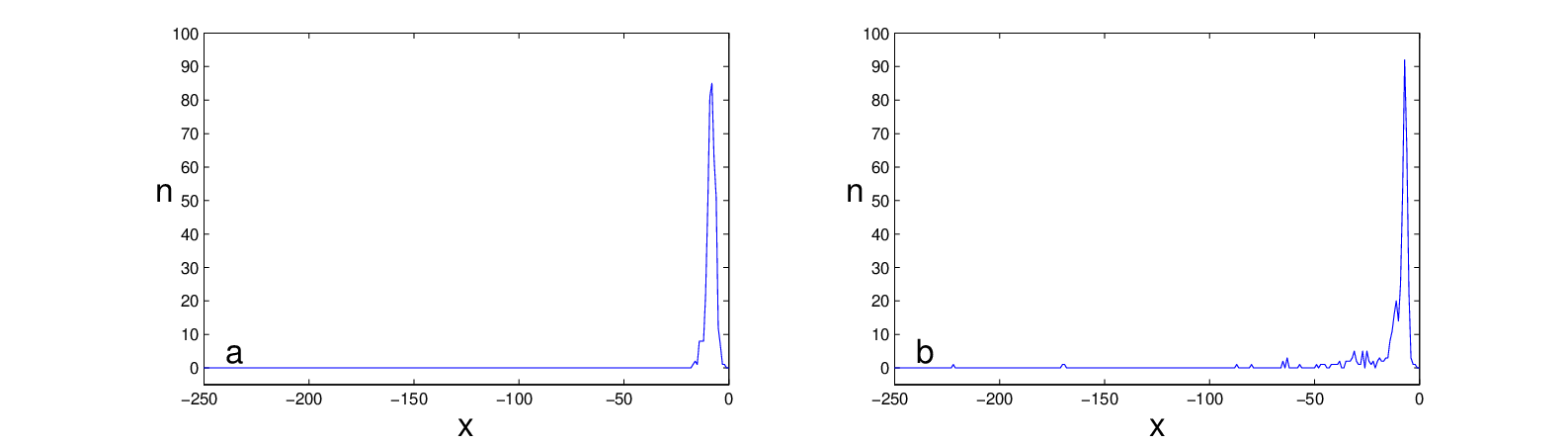
We also examine in each case the lattice site where the filtering is applied. The zero position is defined as the rightmost lattice site with at each time step and the position of the filtering is measured relative to this site. The occurrences at each relative position are then summed over the experiment. We can see (Fig. 4) that the majority of filtering takes place on the shock. However, in the low viscosity case, we observe that at a small number of time steps the filtered site moves significantly ‘behind’ the shockwave.
7 Conclusion
We present three main conclusions from this study.
- 1.
- 2.
In order to clean up the parasite dispersive oscillations in the Lattice Boltzmann method it is necessary to filter the entropy in some way, so as to reduce the extremely-localised incidents of high non-equilibrium entropy; see [5]. Previously reported smoothing of shocks must have been via the inadvertent introduction of numerical dissipation. (Perhaps, this conclusion could be extended to all known regularisers of LBM, including those proposed by ourselves in [4].)
- 3.
For the 1D shock tube, one only needs to filter the entropy at one point per time step (usually very local to the shock), even at very low viscosity, in order to effectively eliminate the post-shock oscillation. We can expect that in 2D and 3D shocks it will be also necessary to filter nonequilibrium entropy in some local maxima points near the shock front only. The entropy filtering for non-entropic equilibria is possible [5] with use of the Kullback–Leibler distance from current distribution to equilibrium (the relative entropy).
The Matlab code used to produce these results is provided in the appendix.
References
- [1] S. Ansumali, I. V. Karlin, Stabilization of the Lattice Boltzmann method by the -theorem: A numerical test, Phys. Rev. E, 62 (6):7999–8003, 2000.
- [2] R. Benzi, S. Succi, and M. Vergassola, The lattice Boltzmann-equation – theory and applications, Phys. Reports, 222:145–197, 1992.
- [3] B. M. Boghosian, P. J. Love, and J. Yepez, Entropic lattice Boltzmann model for Burgers equation, Phil. Trans. Roy. Soc. A, 362:1691–1702, 2004.
- [4] R. A. Brownlee, A. N. Gorban, and J. Levesley, Stability and stabilization of the lattice Boltzmann method, Phys. Rev. E, 75:036711, 2007.
- [5] R. A. Brownlee, A. N. Gorban, and J. Levesley, Nonequilibrium entropy limiters in lattice Boltzmann methods, Physica A, 387 (2-3):385–406, 2008.
- [6] S. K. Godunov, A Difference Scheme for Numerical Solution of Discontinuous Solution of Hydrodynamic Equations, Math. Sbornik, 47:271–306, 1959.
- [7] A. N. Gorban, Basic types of coarse-graining, In: A. N. Gorban, N. Kazantzis, I. G. Kevrekidis, H.-C. Öttinger, and C. Theodoropoulos (eds.), Model Reduction and Coarse-Graining Approaches for Multiscale Phenomena, pages 117–176. Springer, Berlin-Heidelberg-New York, 2006. cond-mat/0602024.
- [8] I. V. Karlin, A. Ferrante, and H. C. Öttinger, Perfect entropy functions of the lattice Boltzmann method, Europhys. Lett. 47:182–188, 1999.
- [9] I. V. Karlin, A. N. Gorban, S. Succi, and V. Boffi, Maximum entropy principle for lattice kinetic equations, Phys. Rev. Lett., 81:6–9, 1998.
- [10] P. D. Lax, On dispersive difference schemes, Phys. D, 18:250–254, 1986.
- [11] C. D. Levermore and J.-G. Liu, Large oscillations arising in a dispersive numerical scheme, Physica D 99:191–216, 1996.
- [12] S. Succi, The lattice Boltzmann equation for fluid dynamics and beyond, Oxford University Press, New York, 2001.
- [13] E. Tadmor and W. Zhong, Entropy stable approximations of Navier–Stokes equations with no artificial numerical viscosity, J. Hyberbolic Differ. Equ., 3:529–559, 2006.
- [14] W.-A. Yong and L.-S. Luo, Nonexistence of theorems for the athermal lattice Boltzmann models with polynomial equilibria, Phys. Rev. E, 67:051105.