跳到论文正文
W Papers独立论文阅读器 arXiv:0901.0769 论文正文 计算阅读时间 · 0%
引用这篇论文根据当前论文元数据生成,正式投稿前建议核对。


License: arXiv.org perpetual non-exclusive license
arXiv:0901.0769v8 [physics.optics] 18 Mar 2009

Energy harvesting by utilization of nanohelices

Sung Nae Cho Email: sungnae.cho@samsung.com Affiliation: MEMS & Packaging Group, Samsung Advanced Institute of Technology, Mt. 14-1 Nongseo-dong Giheung-gu, Yongin-si Gyeonggi-do, 446-712, South Korea
Revised 18 March 2009
Abstract

An energy harvesting device based on nanohelices is presented. The energy harvesting scheme based on nanohelices involves the same rectification circuitry found in many household electronic goods, which converts alternating current (AC) from a wall outlet into a direct current (DC) supply. The presented device, however, involves the rectification of ambient electromagnetic waves rather than the AC source from a household wall outlet.

pacs
41.20.-q, 42.88.+h

I Introduction

Antennas are common in many wireless devices, such as cordless phones, radios, and television sets. For radio and telecommunication applications, antennas are designed to receive electromagnetic waves in the gigahertz frequency ranges. The electromagnetic signals received are converted into electrical currents, which in turn generate sound, images, and so on depending on the type of device. In principle, antennas are the most fundamental energy harvesting devices.

The idea of collecting solar energy by antenna dates back as early as 1970’s1. Since then, researches in solar energy collection by antennas have slowly progressed2, 3, 4, 5. However, due to the limitations on physical size of antenna, it was only recently a significant achievement in energy harvesting by antennas has been realized for the infrared (IR) spectrum of electromagnetic waves6. For telecommunication applications, dimension of antenna is on the order of centimeters. For the IR spectrum of electromagnetic energies, the antenna size scales on the order of sub-microns and this makes harvesting energy from light by antenna even more challenging.

The efficiency of an antenna strongly depends on its size7. With the advent of nanotechnology, the abundance of sub-micron sized structures which can be used as antenna exists today. Nano structures, such as nanorods, nanotubes, and nanodots, are beginning to shed some light on harvesting energy from electromagnetic radiation in IR to ultraviolet (UV) spectrum of range8, 9, 10. The size (or dimension) is not the only physical property that affects the efficiency of an antenna. For more sophisticated antennas, its geometrical configuration, e.g., shape, significantly affects the antenna efficiency7. Antennas based on simple nanorods, nanotubes, or nanodots leave little room for manipulating their geometrical configurations for optimizations. This put helical antennas out of the picture for developing solar cells based on antenna theory. This is all about to change with recent developments in nanohelices11, 12, 13, 14, 15, 16.

The helical antennas are widely deployed technology, which is well documented and studied in literature17, 18. Perhaps, the most widely deployed helical antenna, but which is also least likely to be thought of as one, i.e., as an helical antenna, is the transformer found in many electronic appliances. Because majority of battery operated electronic devices run on direct current (DC) power, the electromagnetic energy harvested by an antenna, which is an alternating current (AC) power, must be rectified. The circuitry that rectifies an AC into a DC power is referred to as a rectifier and one of the breed of rectifiers, a half-wave rectifier, is illustrated in Fig. 1.

Refer to caption
Figure 1: Half-wave rectifier with capacitor.

The AC source in the rectifier circuit is physically represented by a transformer, Fig. 2. The primary and secondary coils are labeled as Pc and Sc, respectively. Basically, transformer is an union of two helical conductors in close proximity, where one of them is termed primary coil and the other is termed secondary coil. Making analogy with the radio station and a radio, the primary coil plays the role of radio station and the secondary coil plays the role of a radio. In a transformer, primary coil transmits electromagnetic waves and the secondary coil receives those waves and converts them into electrical currents.

Refer to caption
Figure 2: Representation of a transformer as the AC source.

The term rectification becomes meaningless unless the output voltage, Vload,V_{\textup{load}}, and the input voltage, Vin,V_{\textup{in}}, satisfy the rectification condition,

Vin\displaystyle V_{\textup{in}} ≥Vload+Vbe,\displaystyle\geq V_{\textup{load}}+V_{\textup{be}}, (1)

where VbeV_{\textup{be}} is the voltage drop across the diode and VinV_{\textup{in}} is the voltage amplitude of the AC source11 1 For the full-wave bridge rectification, the VbeV_{\textup{be}} is replaced by 2​Vbe.2V_{\textup{be}}.. The smaller magnitude for VbeV_{\textup{be}} translates into higher system efficiency. For normal diodes, VbeV_{\textup{be}} ranges between 0.6∼1.80.6\sim 1.8 volts. Schottky diode, which is a special type of diode with very low forward-voltage drop, has the VbeV_{\textup{be}} between approximately 0.1∼0.50.1\sim 0.5 volts.

The household wall outlet supplies anywhere from 115​V115\,\textup{V} to 220​V220\,\textup{V} for Vin,V_{\textup{in}}, which is much larger than the diode forward voltage drop. Therefore, VbeV_{\textup{be}} of 0.6∼1.80.6\sim 1.8 volts is not of much concern when rectifying power line voltage. But, is this the same case for rectification involving ambient electromagnetic waves? To answer this, I shall consider a simple rectenna illustrated in Fig. 3.

Refer to caption
Figure 3: Simple nanorod rectenna, i.e., “rectifying antenna.”

An ambient electromagnetic plane wave with EP≡‖𝐄P‖E_{\textup{P}}\equiv\left\|\mathbf{E}_{\textup{P}}\right\| for the magnitude of its electric field part produces intensity II given by

I=12​c​ε0​EP2,\displaystyle I=\frac{1}{2}c\varepsilon_{0}E_{\textup{P}}^{2}, {c≈3×10⁸​m​s−1,ε0≈8.9×10⁻¹²​s4​A2​m−3​kg−1,\displaystyle\left\{\begin{array}[]{c}c\approx 3\times 10^{8}\,\textup{m}\,\textup{s}^{-1},\\ \varepsilon_{0}\approx 8.9\times 10^{-12}\,\textnormal{{s}}^{4}\,\textnormal{{A}}^{2}\,\textnormal{{m}}^{-3}\,\textnormal{{kg}}^{-1},\end{array}\right.

where cc is the speed of light in vacuum, ε0\varepsilon_{0} is the permittivity of free space, and 𝐄P\mathbf{E}_{\textup{{P}}} is the electric field19. In general, the radiation from sun or nearby heat source does not form plane waves. However, if the longest dimension of the nanorod is comparable to the wavelength of incidence wave, the incidence wave can be approximated as a plane wave20. The intensity of one watt per squared meters corresponds to the electric field magnitude of

I=1​W​m−2,\displaystyle I=1\,\textup{W}\,\textup{m}^{-2}, EP≈2.7×10⁻⁸​V​nm−2.\displaystyle E_{\textup{P}}\approx 2.7\times 10^{-8}\,\textup{V}\,\textup{nm}^{-2}.

For the nanorod of length l,l, the electromotive force (EMF) generated inside of it would be given by

VEMF\displaystyle V_{\textup{EMF}} =∫0l𝐄P⋅𝐝𝐥=EP​l,\displaystyle=\int_{0}^{l}\mathbf{E}_{\textup{{P}}}\cdot\mathbf{dl}=E_{\textup{P}}l,

where, for simplicity, 𝐄P\mathbf{E}_{\textup{P}} has been assumed to be parallel to the length of nanorod. For the nanorod of 1​um1\,\textup{um} in length, intensity of 1​W​m−21\,\textup{W}\,\textup{m}^{-2} generates

VEMF≈2.7×10⁻⁵​VV_{\textup{EMF}}\approx 2.7\times 10^{-5}\,\textup{V}

inside the nanorod. The VEMFV_{\textup{EMF}} generated inside the nanorod rectenna can be identified with the VinV_{\textup{in}} of Fig. 1 and the rectification condition, Eq. (1), gives

2.7×10⁻⁵​V≥Vload+Vbe.2.7\times 10^{-5}\,\textup{V}\geq V_{\textup{load}}+V_{\textup{be}}.

But, this cannot be satisfied for any Vload≥0V_{\textup{load}}\geq 0 even with a Schottky diode, which is known to have very low forward-voltage drop. Can VEMFV_{\textup{EMF}} be amplified so that the rectification condition, Eq. (1), is satisfied for sufficiently large Vload​?V_{\textup{load}}? The answer is yes and this involves the secondary radiation process, which is illustrated in Fig. 4.

Refer to caption
Figure 4: Amplification of VEMFV_{\textup{EMF}} by secondary radiation process.

The irradiance from ambient source, which is indicated by 𝐄P\mathbf{E}_{\textup{{P}}} (electric field part) in the figure, induces radiation from the primary coil, Pc, which is indicated by 𝐄rad\mathbf{E}_{\textup{{rad}}} (electric field part only). Solution obtained by solving Maxwell equations shows that 𝐄rad≫𝐄P\mathbf{E}_{\textup{{rad}}}\gg\mathbf{E}_{\textup{{P}}} when the secondary coil, Sc, is placed very close to the primary coil. Since 𝐄rad\mathbf{E}_{\textup{{rad}}} acts as the incidence wave for Sc, the VEMFV_{\textup{EMF}} is amplified in Sc by factor of 𝐄rad/𝐄P.\mathbf{E}_{\textup{{rad}}}/\mathbf{E}_{\textup{{P}}}.

The amplification of VEMFV_{\textup{EMF}} by secondary radiation process can be qualitatively understood by recalling the multiple-slit experiment with coherent light source, Fig. 5. When plane waves pass through a multiple-slit plate, at distance xx away from the slits, wavelets couple either constructively or destructively depending on the location of yy and this results in bright and dark intensity patterns on screen. The cross-section of nanohelix, which forms the primary and the secondary coils in Fig. 4, resembles the multiple-slit plate (except here, the slit pattern is in ordered zigzag form).

Refer to caption
Figure 5: Multiple-slit diffraction.

That being said, the plane wave condition and the coherence of incidence wave is crucial to the amplification of VEMFV_{\textup{EMF}} by secondary radiation process. The outdoor sun-light or the irradiance from light-bulb are not plane waves if plane waves are thought of as wave front with definite degree of coherence, which can be measured by the visibility of interference20. To put it simply, the degree of coherence is a measure of how perfectly the waves can cancel due to destructive interference (or the opposite, measure of how perfectly the waves can add up due to constructive interference). The coherence was originally introduced in connection with Young’s double-slit experiment in optics, where the interference becomes visible when light is allowed to pass through small aperture such as pin-hole and the effect becomes more pronounced with smaller pin-holes regardless of the light source. Young’s experiment justifies the use of plane wave input for nanohelices considered here as its height and winding pitch scales on the order of wavelength22 2 The winding pitch for the typical nanohelices are several orders or more smaller than the wavelength of the incidence wave..

II Nanotransformer energy harvesting device

II.1 Device structure

The physical layout of energy harvesting device based on nanohelices (or nanotransformer21, 22) is illustrated in Fig. 6 and its equivalent circuit diagram is provided in Fig. 7. Borrowing the terminology from display technology, I shall refer to each element in diode layer (indicated by N-type and P-type square pairs in Fig. 6) and nanohelices making contact with the diode element as a pixel. For clarity, the pixel is indicated by dotted rectangular three dimensional cube in Fig. 8.

Refer to caption
Figure 6: Nanotransformer energy harvesting device layout.
Refer to caption
Figure 7: Equivalent circuitry.

The proposed energy harvesting device based on nanohelices involves three major device layers (capacitor, diode, and nanohelix layers), which can be processed independently and sandwiched together for the final product, Fig. 8. Such process allows manufacturing of the proposed energy harvesting device at large scales.

Refer to caption
Figure 8: Three major layers of nanotransformer energy harvesting device.

The diode layer can be first prepared as a one large sheet of a diode, which then can be patterned to form pixels of diodes. The nanohelix layer in current device scheme can be prepared by growing helices in normal direction of the substrate as illustrated in Fig. 9. Equivalently, nanohelices can also be spin coated directly onto the surface of a substrate. In this case, nanohelices would most likely be positioned with its length parallel to the surface of a substrate. To prevent diode layer from collapsing onto the substrate of nanohelix layer, transparent dielectric spacer such as SiO2\textup{Si}\textup{O}_{2} nanoparticles may be distributed on the substrate surface as illustrated in Figs. 9 and 10.

Refer to caption
Figure 9: Schematic of grown nanohelices.
Refer to caption
Figure 10: The cross-sectional view of nanohelix layer with diode layer placed over it.

II.2 Operation principle

For a successful rectification, the VEMFV_{\textup{EMF}} generated across each pixel must be amplified large enough to satisfy the rectification condition, Eq. (1). As already discussed in previous sections, the amplification of VEMFV_{\textup{EMF}} is achieved thru the process of secondary amplification, recall Fig. 4. The role of primary coil, i.e., Pc in Fig. 4, in current device scheme, Figs. 6 and 7, is played out by nanohelices belonging to the neighboring pixels. Due to constructive and destructive interferences of wavelets originating from different nanohelices, there would be pixels receiving amplified radiation fields and there would be those pixels receiving virtually no radiation fields. Only those pixels positioned in locations where constructive interference occurs would generate large enough VEMFV_{\textup{EMF}} to meet the rectification condition and, eventually, participate in energy harvesting.

The number of pixels, where a pixel is indicated by dotted rectangular three dimensional cube in Fig. 8, plays the key role in the energy harvesting based on nanohelices. As an illustration, assume that each pixel has a dimension of 10​um×10​um10\,\textup{um}\times 10\,\textup{um} for its surface area. In an ideal close packing, about 100100 million such pixels would be able to fit in an area of 10​cm×10​cm.10\,\textup{cm}\times 10\,\textup{cm}. Weber et al. have experimentally shown that ZnO nanowire can carry up to roughly 330​nA330\,\textup{nA} of electrical current before it snaps23. The current limiting resistors in Figs. 4, 6, and 7 prevents the overloading of nanohelices with too much current, thereby saving it from a break down. If assumed that each pixel contains single nanohelix and that each nanohelix carries electrical current of 130​nA,130\,\textup{nA}, this amounts to a total of 13​A13\,\textup{A} out of the device. Of course, only those pixels positioned in locations where constructive interference occurs to generate VEMFV_{\textup{EMF}} large enough to meet the rectification condition contribute to the total current. But, even if one assumes that only 10%10\% of 100100 million pixels contribute in energy harvesting, this still yields the total of 1.3​A1.3\,\textup{A} from the device.

Having said enough about the potential of energy harvesting based on nanohelices, the validity of working principles behind the proposed device depend heavily on the amplification of ambient electromagnetic fields by secondary radiation process, thru which process generates VEMFV_{\textup{EMF}} large enough to satisfy the rectification condition. Since the amplification of VEMFV_{\textup{EMF}} depends on both magnetic induction ( 𝐁rad\mathbf{B}_{\textup{{rad}}} ) and electric field ( 𝐄rad\mathbf{E}_{\textup{{rad}}} ) parts of the electromagnetic radiation from the primary helix,

VEMF∝{‖𝐄rad‖‖𝐁rad‖,V_{\textup{EMF}}\propto\left\{\begin{array}[]{c}\left\|\mathbf{E}_{\textup{{rad}}}\right\|\\ \left\|\mathbf{B}_{\textup{{rad}}}\right\|\end{array}\right.,

one needs to quantitatively show that indeed 𝐄rad\mathbf{E}_{\textup{{rad}}} and 𝐁rad\mathbf{B}_{\textup{{rad}}} get amplified significantly,

EradEP≡‖𝐄rad‖‖𝐄P‖≫1,\displaystyle\frac{E_{\textup{rad}}}{E_{\textup{P}}}\equiv\frac{\left\|\mathbf{E}_{\textup{{rad}}}\right\|}{\left\|\mathbf{E}_{\textup{{P}}}\right\|}\gg 1, BradBP≡‖𝐁rad‖‖𝐁P‖≫1.\displaystyle\frac{B_{\textup{rad}}}{B_{\textup{P}}}\equiv\frac{\left\|\mathbf{B}_{\textup{{rad}}}\right\|}{\left\|\mathbf{B}_{\textup{{P}}}\right\|}\gg 1. (3)

The quantitative verification of Eq. (3) involves the solving of Maxwell equations and this is the task which I set out to do in the next sections.

III Theory

All phenomena involving interaction with electromagnetic waves involve Maxwell equations. To keep the topic presented here self-contained, I shall briefly summarize the kind of manipulations and approximations assumed in obtaining the vector potential partial differential equation (PDE), which marks the starting point for the rest of analysis throughout this presentation.

III.1 Maxwell equations

Maxwell equations, in the form independent of particular system of units, may be expressed as

∇⋅𝐄=4​π​g​ρ,\displaystyle\nabla\cdot\mathbf{E}=4\pi g\rho, ∇⋅𝐁=0,\displaystyle\nabla\cdot\mathbf{B}=0,
∇×𝐄=−η​∂𝐁∂t,\displaystyle\nabla\times\mathbf{E}=-\eta\frac{\partial\mathbf{B}}{\partial t}, ∇×𝐁=4​π​γ​𝐉+γg​∂𝐄∂t,\displaystyle\nabla\times\mathbf{B}=4\pi\gamma\mathbf{J}+\frac{\gamma}{g}\frac{\partial\mathbf{E}}{\partial t},

where ρ\rho is the total charge density, 𝐉\mathbf{J} is the total current density, 𝐁\mathbf{B} is the magnetic induction, 𝐄\mathbf{E} is the electric field, and the positive constants g,g, γ,\gamma, and η\eta depend on the particular system of units being adopted24. If one assumes that both charge and current densities are specified throughout space and assume that 𝐄,\mathbf{E}, 𝐁,\mathbf{B}, ρ,\rho, and 𝐉\mathbf{J} vary in time as exp⁡(i​ω​t),\exp\left(i\omega t\right), Maxwell equations may be re-expressed in an alternate form as

∇⋅𝐄=4​π​g​ρ,\displaystyle\nabla\cdot\mathbf{E}=4\pi g\rho, ∇⋅𝐁=0,\displaystyle\nabla\cdot\mathbf{B}=0,
∇×𝐄=−i​ω​η​𝐁,\displaystyle\nabla\times\mathbf{E}=-i\omega\eta\mathbf{B}, ∇×𝐁=4​π​γ​𝐉+i​ω​γg​𝐄,\displaystyle\nabla\times\mathbf{B}=4\pi\gamma\mathbf{J}+\frac{i\omega\gamma}{g}\mathbf{E},

where ω\omega is the angular frequency. For a non-static case, where ω≠0,\omega\neq 0, the electric divergence relation,

∇⋅𝐄=4​π​g​ρ,\nabla\cdot\mathbf{E}=4\pi g\rho,

becomes redundant33 3 The redundancy of ∇⋅𝐄=4​π​g​ρ\nabla\cdot\mathbf{E}=4\pi g\rho for ω≠0\omega\neq 0 can be shown by taking the divergence of ∇×𝐁,\nabla\times\mathbf{B}, ∇⋅∇×𝐁=4πγ∇⋅𝐉+i​ω​γg∇⋅𝐄=0\nabla\cdot\nabla\times\mathbf{B}=4\pi\gamma\nabla\cdot\mathbf{J}+\frac{i\omega\gamma}{g}\nabla\cdot\mathbf{E}=0 to yield i​ω​γg∇⋅𝐄=−4πγ∇⋅𝐉.\frac{i\omega\gamma}{g}\nabla\cdot\mathbf{E}=-4\pi\gamma\nabla\cdot\mathbf{J}. Finally, insertion of the continuity equation, ∇⋅𝐉=−i​ω​ρ,\nabla\cdot\mathbf{J}=-i\omega\rho, proves the result, i​ω​γg∇⋅𝐄=iωγ4πρ⇒∇⋅𝐄=4πgρ.\frac{i\omega\gamma}{g}\nabla\cdot\mathbf{E}=i\omega\gamma 4\pi\rho\Rightarrow\nabla\cdot\mathbf{E}=4\pi g\rho. and the problem of electrodynamics is reduced to solving the following set of Maxwell equations in harmonic frequency domain,

∇⋅𝐁\displaystyle\nabla\cdot\mathbf{B} =0,\displaystyle=0, (4)
∇×𝐄\displaystyle\nabla\times\mathbf{E} =−i​ω​η​𝐁,\displaystyle=-i\omega\eta\mathbf{B}, (5)
∇×𝐁\displaystyle\nabla\times\mathbf{B} =4​π​γ​𝐉+i​ω​γg​𝐄.\displaystyle=4\pi\gamma\mathbf{J}+\frac{i\omega\gamma}{g}\mathbf{E}. (6)

III.2 Vector potential

I proceed by seeking a vector field solution that simultaneously satisfies Maxwell equations (4) thru (6). Any vector field 𝐀,\mathbf{A}, which satisfies the condition

𝐁=∇×𝐀,\mathbf{B}=\nabla\times\mathbf{A}, (7)

automatically satisfies Eq. (4) and such vector 𝐀\mathbf{A} is given a name “vector potential.” Substitution of Eq. (7) in Eq. (5) gives

∇×(𝐄+i​ω​η​𝐀)=0.\nabla\times\left(\mathbf{E}+i\omega\eta\mathbf{A}\right)=0.

The fundamental theorem of vector analysis tells us that any scalar field Φ\Phi satisfies the condition ∇×∇Φ=0.\nabla\times\nabla\Phi=0. And, this implies

𝐄+i​ω​η​𝐀=∇Φ,\mathbf{E}+i\omega\eta\mathbf{A}=\nabla\Phi,

where the sign of Φ\Phi is arbitrary. However, because it has already been defined in literature that 𝐄=−∇Φ\mathbf{E}=-\nabla\Phi for the static limit, where ω=0,\omega=0, one chooses Φ→−Φ\Phi\rightarrow-\Phi for the scalar field and the previous relation becomes

𝐄=−i​ω​η​𝐀−∇Φ.\mathbf{E}=-i\omega\eta\mathbf{A}-\nabla\Phi. (8)

Equation (8) automatically becomes the static limit expression in the limit ω\omega goes to zero.

The concept of vector and scalar fields simplify electromagnetic problem to solving of a single Maxwell equation (6). Insertion of Eqs. (7) and (8) into Eq. (6) gives

∇×∇×𝐀=4πγ𝐉+i​ω​γg(−iωη𝐀−∇Φ).\nabla\times\nabla\times\mathbf{A}=4\pi\gamma\mathbf{J}+\frac{i\omega\gamma}{g}\left(-i\omega\eta\mathbf{A}-\nabla\Phi\right).

Application of the vector identity,

∇×∇×𝐀=−∇2𝐀+∇(∇⋅𝐀),\nabla\times\nabla\times\mathbf{A}=-\nabla^{2}\mathbf{A}+\nabla\left(\nabla\cdot\mathbf{A}\right),

transforms the previous relation as

∇2𝐀−∇(∇⋅𝐀)=−4πγ𝐉−ω2​γ​ηg𝐀+i​ω​γg∇Φ.\nabla^{2}\mathbf{A}-\nabla\left(\nabla\cdot\mathbf{A}\right)=-4\pi\gamma\mathbf{J}-\frac{\omega^{2}\gamma\eta}{g}\mathbf{A}+\frac{i\omega\gamma}{g}\nabla\Phi.

After some rearrangements, I arrive at the expression,

∇(∇⋅𝐀+i​ω​γg​Φ)=∇2𝐀+ω2​γ​ηg​𝐀+4​π​γ​𝐉.\nabla\left(\nabla\cdot\mathbf{A}+\frac{i\omega\gamma}{g}\Phi\right)=\nabla^{2}\mathbf{A}+\frac{\omega^{2}\gamma\eta}{g}\mathbf{A}+4\pi\gamma\mathbf{J}. (9)

Since any 𝐀\mathbf{A} and Φ\Phi satisfying Eq. (7) and Eq. (8), respectively, solves Eq. (9), one is free to choose any convenient 𝐀\mathbf{A} and Φ\Phi so that Eq. (9) becomes solvable. Choosing the following expression for Φ,\Phi,

Φ=i​gω​γ∇⋅𝐀,\Phi=\frac{ig}{\omega\gamma}\nabla\cdot\mathbf{A}, (10)

makes the left side of Eq. (9) to vanish. And, the electric field, utilizing Eq. (8), can be expressed as

𝐄=−iωη𝐀−i​gω​γ∇(∇⋅𝐀).\mathbf{E}=-i\omega\eta\mathbf{A}-\frac{ig}{\omega\gamma}\nabla\left(\nabla\cdot\mathbf{A}\right). (11)

With Φ\Phi defined in Eq. (10), the vector potential satisfies the following partial differential equation (PDE),

∇2𝐀+g2​𝐀=−4​π​γ​𝐉,K=ω​γ​ηg>0,\nabla^{2}\mathbf{A}+g^{2}\mathbf{A}=-4\pi\gamma\mathbf{J},\quad K=\omega\sqrt{\frac{\gamma\eta}{g}}>0, (12)

where the constant KK has the physical implication of being the wave number. Equation (12) is the well known Helmholtz equation and its solution is given by

𝐀⁡(𝐑)=γ​∭𝐉​exp⁡(−i​K​‖𝐑−𝐑s‖)‖𝐑−𝐑s‖​d​Vs,\mathbf{A}\left(\mathbf{R}\right)=\gamma\iiint\frac{\mathbf{J}\exp\left(-iK\left\|\mathbf{R}-\mathbf{R}_{\textup{s}}\right\|\right)}{\left\|\mathbf{R}-\mathbf{R}_{\textup{s}}\right\|}dV_{\textup{s}}, (13)

where 𝐑s\mathbf{R}_{\textup{s}} is the position of current density, 𝐉≡𝐉⁡(𝐑s),\mathbf{J}\equiv\mathbf{J}\left(\mathbf{R}_{\textup{s}}\right), and the volume integration is performed over entire region containing the current source.

IV Analysis

IV.1 Nanohelix

The simplest solenoid is given by a non-planar helical curve depicted in Fig. 11. If 𝐞1,\mathbf{e}_{1}, 𝐞2,\mathbf{e}_{2}, and 𝐞3\mathbf{e}_{3} denote a right-handed system of mutually perpendicular unit vectors, then every spatial points on filamentary finite helix can be represented by

𝐑s=𝐑o+𝐑′,\mathbf{R}_{\textup{s}}=\mathbf{R}_{\textup{o}}+\mathbf{R}^{\prime}, (14)

where 𝐑o\mathbf{R}_{\textup{o}} is the position vector defining the local origin O′O^{\prime} and 𝐑′\mathbf{R}^{\prime} is the vector defining the position of current source relative to O′.O^{\prime}. In Cartesian coordinates, 𝐑′\mathbf{R}^{\prime} and 𝐑o\mathbf{R}_{\textup{o}} are given by

(𝐑′𝐑o)=∑i=13(xi′xo​i)​𝐞i,{x1′≡x′=a​cos⁡s,x2′≡y′=a​sin⁡s,x3′≡z′=b​s.\left(\begin{array}[]{c}\mathbf{R}^{\prime}\\ \mathbf{R}_{\textup{o}}\end{array}\right)=\sum_{i=1}^{3}\left(\begin{array}[]{c}x_{i}^{\prime}\\ x_{\textup{o}i}\end{array}\right)\mathbf{e}_{i},\quad\left\{\begin{array}[]{c}x_{1}^{\prime}\equiv x^{\prime}=a\cos s,\\ x_{2}^{\prime}\equiv y^{\prime}=a\sin s,\\ x_{3}^{\prime}\equiv z^{\prime}=bs.\end{array}\right. (15)

For the rest of the presentation, I shall designate the trio (𝐞1,𝐞2,𝐞3)\left(\mathbf{e}_{1},\mathbf{e}_{2},\mathbf{e}_{3}\right) with (x,y,z)\left(x,y,z\right) in respective order. Similarly, for the O′O^{\prime} coordinates, I shall designate the trio (𝐞1,𝐞2,𝐞3)\left(\mathbf{e}_{1},\mathbf{e}_{2},\mathbf{e}_{3}\right) with (x′,y′,z′)\left(x^{\prime},y^{\prime},z^{\prime}\right) in respective order. The coordinates x′x^{\prime} and y′y^{\prime} describe a circle of radius a,a, and the z′,z^{\prime}, which coordinate defines the height of finite helix, increases or decreases in direct proportion to the parameter s.s. The vertical distance between the coils, which is known as the pitch, equals the increase in z′z^{\prime} as ss jumps by 2​π.2\pi. The pitch is hence given by

pitch=2​π​b.\textnormal{pitch}=2\pi b. (16)
Refer to caption
Figure 11: Finite helix, where 𝐞1|x|x′,\mathbf{e}_{1}\parallel x\parallel x^{\prime}, 𝐞2|y|y′,\mathbf{e}_{2}\parallel y\parallel y^{\prime}, and 𝐞3|z|z′.\mathbf{e}_{3}\parallel z\parallel z^{\prime}. The symbol ∥\parallel reads as “parallel to.”

Assuming 𝐑s\mathbf{R}_{\textup{s}} is differentiable and that 𝐑o\mathbf{R}_{\textup{o}} does not depend on parameter s,s, the vector which is tangent to the curve defining the finite helix is given by

𝐓≡d​𝐑sd​s=∑i=13Ti​𝐞i,\mathbf{T}\equiv\frac{d\mathbf{R}_{\textup{s}}}{ds}=\sum_{i=1}^{3}T_{i}\mathbf{e}_{i}, (17)

where

T1=−a​sin⁡s,T2=a​cos⁡s,T3=b.T_{1}=-a\sin s,\quad T_{2}=a\cos s,\quad T_{3}=b. (18)

The total length, l,l, of filamentary finite helical curve is found by taking the line integration of associated tangent vector with respect to the parameter s,s,

l\displaystyle l =∫𝐓⋅𝑑𝐬=∫‖𝐓‖​𝑑s=s​a2+b2,\displaystyle=\int\mathbf{T}\cdot d\mathbf{s}=\int\left\|\mathbf{T}\right\|ds=s\sqrt{a^{2}+b^{2}},

where d​𝐬d\mathbf{s} is the differential arc length of the finite helix segment. One thus obtains the upper limit for the parameter s,s,

c=la2+b2,0<s≤c.c=\frac{l}{\sqrt{a^{2}+b^{2}}},\quad 0<s\leq c. (19)

With the parameter s,s, the entire height of finite helix is given by b​cbc or b​l/a2+b2bl/\sqrt{a^{2}+b^{2}} as indicated in Fig. (11).

The vector potential integral of Eq. (13) is integrated over the entire volume containing the current sources. If the current sources are confined to a filamentary finite helix whose spatial curve is represented by Eq. (14), the helix may be partitioned into segments of finite but equal sizes as illustrated in Fig. 12. The filamentary wire forming finite helix has a length of l.l. Within the representation parametrized in s,s, each of NN segments has length of c/N,c/N, where cc is defined in Eq. (19). The number of segments is arbitrary, as one can slice the wire into as many pieces as he or she wants to. To make the argument more concise, the filamentary wire is sliced into enough segments so that 𝐉\mathbf{J} for the segment is a constant and the entire segment is identified with its center, 𝐑s​n,\mathbf{R}_{\textup{s}n}, on the finite helix. Then, for a detector placed at location 𝐑,\mathbf{R}, the detected vector potential, which has been contributed from the segment nn on the finite helix, gets approximated by the expression

𝐀n≈γ​αn​cN​∭δ⁡(𝐑s−𝐑s​n)​exp⁡(−i​K​‖𝐑−𝐑s‖)‖𝐑−𝐑s‖​𝑑V,\mathbf{A}_{n}\approx\frac{\gamma\alpha_{n}c}{N}\iiint\frac{\delta\left(\mathbf{R}_{\textup{s}}-\mathbf{R}_{\textup{s}n}\right)\exp\left(-iK\left\|\mathbf{R}-\mathbf{R}_{\textup{s}}\right\|\right)}{\left\|\mathbf{R}-\mathbf{R}_{\textup{s}}\right\|}dV, (20)

where the volume integration is over all space, the quantity c/Nc/N represents the length of segment, the constant αn\alpha_{n} is related to the local current density 𝐉n\mathbf{J}_{n} for the n​thn\textnormal{th} segment by 𝐉n=c​αn/N,\mathbf{J}_{n}=c\alpha_{n}/N, and δ⁡(𝐑s−𝐑s​n)\delta\left(\mathbf{R}_{\textup{s}}-\mathbf{R}_{\textup{s}n}\right) is the Dirac delta function, which has the integral property,

∭f⁡(𝐘)​δ​(𝐘−𝐗)​𝑑V=f⁡(𝐗).\iiint f\left(\mathbf{Y}\right)\delta\left(\mathbf{Y}-\mathbf{X}\right)dV=f\left(\mathbf{X}\right).

Application of the integral property of Dirac delta function on Eq. (20) yields the result

𝐀n≈γ​αn​c​exp⁡(−i​K​‖𝐑−𝐑s​n‖)N​‖𝐑−𝐑s​n‖.\mathbf{A}_{n}\approx\frac{\gamma\alpha_{n}c\exp\left(-iK\left\|\mathbf{R}-\mathbf{R}_{\textup{{s}}n}\right\|\right)}{N\left\|\mathbf{R}-\mathbf{R}_{\textup{{s}}n}\right\|}. (21)

The detector receives contributions from all NN segments of the finite helix, not just from the n​thn\textnormal{th} segment. Therefore, summing over the contributions from all NN segments of the finite helix, I have

𝐀≈∑n=1N𝐀n=∑n=1Nγ​αn​c​exp⁡(−i​K​‖𝐑−𝐑s​n‖)N​‖𝐑−𝐑s​n‖.\mathbf{A}\approx\sum_{n=1}^{N}\mathbf{A}_{n}=\sum_{n=1}^{N}\frac{\gamma\alpha_{n}c\exp\left(-iK\left\|\mathbf{R}-\mathbf{R}_{\textup{{s}}n}\right\|\right)}{N\left\|\mathbf{R}-\mathbf{R}_{\textup{{s}}n}\right\|}.

Finally, in the limit the slices become finer and finer, it becomes

𝐀=limN→∞∑n=1Nγ​αn​c​exp⁡(−i​K​‖𝐑−𝐑s​n‖)N​‖𝐑−𝐑s​n‖.\mathbf{A}=\lim_{N\rightarrow\infty}\sum_{n=1}^{N}\frac{\gamma\alpha_{n}c\exp\left(-iK\left\|\mathbf{R}-\mathbf{R}_{\textup{{s}}n}\right\|\right)}{N\left\|\mathbf{R}-\mathbf{R}_{\textup{{s}}n}\right\|}.

In the representation parametrized by s,s, one notices that c/N=△​sc/N=\triangle s and, as NN goes to infinity, △​s\triangle s becomes infinitesimal, i.e., △​s→d​s.\triangle s\rightarrow ds. Also, as the slices get finer, what was the center point for the n​thn\textnormal{th} slice becomes the exact point for the slice, 𝐑s​n→𝐑s.\mathbf{R}_{\textup{s}n}\rightarrow\mathbf{R}_{\textup{s}}. Similarly, what was an average current density within the slice becomes an exact current density for the point 𝐑s,\mathbf{R}_{\textup{s}}, αn→𝐉⁡(𝐑s).\alpha_{n}\rightarrow\mathbf{J}\left(\mathbf{R}_{\textup{s}}\right). Hence,

limN→∞∑n=1Nf⁡(x)​cN→∫f⁡(x)​𝑑s,\lim_{N\rightarrow\infty}\sum_{n=1}^{N}f\left(x\right)\frac{c}{N}\rightarrow\int f\left(x\right)ds,

and the vector potential expression for the finite helix becomes

𝐀=γ​∫0c𝐉​exp⁡(−i​K​‖𝐑−𝐑s‖)‖𝐑−𝐑s‖​𝑑s,\mathbf{A}=\gamma\int_{0}^{c}\frac{\mathbf{J}\exp\left(-iK\left\|\mathbf{R}-\mathbf{R}_{\textup{s}}\right\|\right)}{\left\|\mathbf{R}-\mathbf{R}_{\textup{s}}\right\|}ds, (22)

where 𝐑s\mathbf{R}_{\textup{s}} is defined in Eq. (14) with its components given by Eq. (15). As the current density, 𝐉,\mathbf{J}, has not been defined, the vector potential integral in parametrized form, Eq. (22), cannot be evaluated. The current density source for the finite helix system is cast into a quantitative form in the next section.

Refer to caption
Figure 12: Segmented finite helix.

IV.2 Induced current

Consider an electromagnetic problem depicted in Fig. 13, where a plane wave front is impinging on the finite helix whose configuration is describe by Eq. (14). The real world solenoid, no matter how small, always has cross-sectional area of finite size which holds current responsible for induced electromagnetic radiation. Modeling a real world solenoid can be difficult due to the complications arising from a finite thickness for the cross-sectional area. However, the mathematical modeling can be substantially simplified by letting the cross-sectional area of the wire to go to zero and, at the same time, letting the current density to go to infinity in such a manner that the flux of current along the wire remains constant. For the current carrying helical wire modeled within such approximation, Eq. (14) suffices for the description of finite solenoid.

Refer to caption
Figure 13: Plane wave incident on finite helix. The Poynting vector is indicated by 𝐒p.\mathbf{S}_{\textup{p}}.

The vector field 𝐀,\mathbf{A}, whose solution satisfies the PDE of Eq. (12), arises as a result of induced current within the finite helix. This induced current inside a finite helix is due to the electric field component of impinging plane wave as illustrated in Fig. 13. Assuming that wire forming finite helix can be represented by an isotropic ohmic conductor, the current density 𝐉\mathbf{J} is given by the Ohm’s law,

𝐉=σ​𝐄p,{σ≡σ⁡(𝐑s),𝐄p≡𝐄p​(𝐑s),\mathbf{J}=\sigma\mathbf{E}_{\textnormal{{p}}},\quad\left\{\begin{array}[]{c}\sigma\equiv\sigma\left(\mathbf{R}_{\textup{s}}\right),\\ \mathbf{E}_{\textnormal{{p}}}\equiv\mathbf{E}_{\textnormal{{p}}}\left(\mathbf{R}_{\textup{s}}\right),\end{array}\right. (23)

where σ\sigma is the electrical conductivity, 𝐄p\mathbf{E}_{\textnormal{{p}}} is the polarization (electric field) of impinging plane wave front, and 𝐑s\mathbf{R}_{\textup{s}} is the position of current source.

Electromagnetic waves have both electric and magnetic field parts, as illustrated in Fig. 14. For a nanohelix whose coil diameter is less than 50​nm,50\,\textup{nm}, an IR range electromagnetic plane wave passing through it would be perceived as a DC magnetic field switching between on and off modes at a rate of wave frequency. This comes about because the wavelength of electromagnetic waves in the IR range scales on the order of microns, which implies the vast majority of IR range electromagnetic waves are more than hundred times larger in their wavelength compared to the 50​nm50\,\textup{nm} diameter of the nanohelix. And, this argument strengthens with nanohelices of smaller diameter size (or with longer wavelengths, for example, microwaves and radio waves).

Refer to caption
Figure 14: The 𝐄p\mathbf{E}_{\textnormal{{p}}} and 𝐁p\mathbf{B}_{\textnormal{{p}}} are electric and magnetic parts of electromagnetic wave, and 𝐒P\mathbf{S}_{\textup{{P}}} is the Poynting vector. The enclosed box shows the time varying flux of magnetic induction enclosed by the nanohelix loop, where the symbol ×\times denotes the case of 𝐁p=−Bp​𝐞3\mathbf{B}_{\textnormal{{p}}}=-B_{\textup{p}}\mathbf{e}_{3} and the symbol ∙\bullet denotes the case of 𝐁p=Bp​𝐞3.\mathbf{B}_{\textnormal{{p}}}=B_{\textup{p}}\mathbf{e}_{3}.

The macroscopic conducting coil driven by a household line voltage alternating at 60​Hz60\,\textup{Hz} generates electromagnetic waves radiating at 60​Hz.60\,\textup{Hz}. Such radiation would have a wavelength of roughly 5000​km5000\,\textup{km} in air, i.e., λ=3×10⁸/60.\lambda=3\times 10^{8}/60. A secondary conductive coil placed nearby it would perceive as if the magnetic part of the radiating electromagnetic wave was a DC magnetic field switching in an empty between on and off modes, except now at the rate of 60​Hz60\,\textup{Hz} cycle. Again, the argument holds because even a solenoid of diameter as large as 100​cm100\,\textup{cm} is still fifty million times small compared to the wavelength of λ=5000​km.\lambda=5000\,\textup{km}.

In summary, the case involving nanohelix and the IR spectrum of electromagnetic waves, in principle, is just the scaled down analogue of the case which involves the interaction between electromagnetic waves radiated by macroscopic conductive primary coil driven by a household line voltage alternating at 60​Hz60\,\textup{Hz} and the secondary solenoid placed nearby.

That being said, under the exposure of electromagnetic radiation, net electric current gets induced inside the nanohelix in accordance with Faraday’s law of induction and the total induced current density inside the nanohelix must be expressed as

𝐉=σ​𝐄p+𝐉B,\mathbf{J}=\sigma\mathbf{E}_{\textnormal{{p}}}+\mathbf{J}_{\textup{B}},

where 𝐉B\mathbf{J}_{\textup{B}} is the induced current density contribution arising from the magnetic part of the incidence ambient electromagnetic wave. Nevertheless, for the analysis here, I neglect 𝐉B\mathbf{J}_{\textup{B}} as this involves very lengthy derivation on its own. However, it is reminded that 𝐉B\mathbf{J}_{\textup{B}} only makes 𝐉\mathbf{J} bigger. Therefore, once I show that Eq. (3) is satisfied even with contribution from 𝐉B\mathbf{J}_{\textup{B}} neglected in 𝐉,\mathbf{J}, redoing the problem with contribution from 𝐉B\mathbf{J}_{\textup{B}} included in 𝐉\mathbf{J} should only make the case even firmer.

Returning from a short detour, in the case where finite helix is made of a filamentary wire, only the component of electric field which is parallel to the local length of wire can induce current as depicted in Fig. 15. The polarization of impinging plane wave can be decomposed into 𝐄p⟂\mathbf{E}_{\textnormal{{p}}\perp} and 𝐄p∥\mathbf{E}_{\textnormal{{p}}\parallel} at the local point 𝐑s\mathbf{R}_{\textup{s}} of the finite helix, where 𝐄p⟂\mathbf{E}_{\textnormal{{p}}\perp} and 𝐄p∥\mathbf{E}_{\textnormal{{p}}\parallel} are the two components of 𝐄p\mathbf{E}_{\textnormal{{p}}} that are, respectively, perpendicular and parallel to the local tangent of finite helix at 𝐑s.\mathbf{R}_{\textup{s}}. In a filamentary wire, only 𝐄p∥\mathbf{E}_{\textnormal{{p}}\parallel} can result in induced current. Mathematically, 𝐄p∥\mathbf{E}_{\textnormal{{p}}\parallel} at local point, 𝐑s,\mathbf{R}_{\textup{s}}, is expressed as

𝐄p∥=(𝐄p⋅𝐓𝐓⋅𝐓)𝐓,{𝐄p≡𝐄p​(𝐑s),𝐓≡𝐓⁡(𝐑s),\mathbf{E}_{\textnormal{{p}}\parallel}=\left(\frac{\mathbf{E}_{\textnormal{{p}}}\cdot\mathbf{T}}{\mathbf{T}\cdot\mathbf{T}}\right)\mathbf{T},\quad\left\{\begin{array}[]{c}\mathbf{E}_{\textnormal{{p}}}\equiv\mathbf{E}_{\textnormal{{p}}}\left(\mathbf{R}_{\textup{s}}\right),\\ \mathbf{T}\equiv\mathbf{T}\left(\mathbf{R}_{\textup{s}}\right),\end{array}\right. (24)

where 𝐓\mathbf{T} is the local tangent vector for finite helix at 𝐑s.\mathbf{R}_{\textup{s}}. The explicit expression for 𝐓\mathbf{T} has already been defined in Eq. (18). Insertion of Eq. (24) for 𝐄p\mathbf{E}_{\textnormal{{p}}} in Eq. (25) ensures that only 𝐄p∥\mathbf{E}_{\textnormal{{p}}\parallel} takes part in the generation of locally induced current density,

𝐉=σ⁡(𝐄p⋅𝐓𝐓⋅𝐓)​𝐓,𝐉≡𝐉⁡(𝐑s).\mathbf{J}=\sigma\left(\frac{\mathbf{E}_{\textnormal{{p}}}\cdot\mathbf{T}}{\mathbf{T}\cdot\mathbf{T}}\right)\mathbf{T},\quad\mathbf{J}\equiv\mathbf{J}\left(\mathbf{R}_{\textup{s}}\right). (25)
Refer to caption
Figure 15: Perpendicular and parallel polarization components at the local helix segment.

Without loss of generality, the electric field of impinging plane wave at points on the finite helix can be expressed as

𝐄p​(𝐑s)=exp⁡(i​𝐊⋅𝐑s+i​ω​t)​∑i=13Ep​i​𝐞i,\mathbf{E}_{\textnormal{{p}}}\left(\mathbf{R}_{\textup{s}}\right)=\exp\left(i\mathbf{K}\cdot\mathbf{R}_{\textup{s}}+i\omega t\right)\sum_{i=1}^{3}E_{\textnormal{{p}}i}\mathbf{e}_{i}, (26)

where the wave vector 𝐊\mathbf{K} is given by

𝐊=∑i=13Ki​𝐞i.\mathbf{K}=\sum_{i=1}^{3}K_{i}\mathbf{e}_{i}. (27)

In terms of the direction cosines,

cosαi=Ep​iEp≡Ep​i‖𝐄p‖,i=1,2,3,\cos\alpha_{i}=\frac{E_{\textnormal{{p}}i}}{E_{\textnormal{{p}}}}\equiv\frac{E_{\textnormal{{p}}i}}{\left\|\mathbf{E}_{\textnormal{{p}}}\right\|},\quad i=1,2,3, (28)

the Eq. (26) can be expressed as

𝐄p=Ep​exp⁡(i​𝐊⋅𝐑s+i​ω​t)​∑i=13cos⁡αi​𝐞i.\mathbf{E}_{\textup{{p}}}=E_{\textnormal{{p}}}\exp\left(i\mathbf{K}\cdot\mathbf{R}_{\textup{s}}+i\omega t\right)\sum_{i=1}^{3}\cos\alpha_{i}\mathbf{e}_{i}. (29)

With the following expressions,

𝐓⋅𝐓\displaystyle\mathbf{T}\cdot\mathbf{T} =a2+b2,\displaystyle=a^{2}+b^{2},
𝐄p⋅𝐓\displaystyle\mathbf{E}_{\textnormal{{p}}}\cdot\mathbf{T} =Ep​χ​exp⁡(i​𝐊⋅𝐑s+i​ω​t),\displaystyle=E_{\textnormal{{p}}}\chi\exp\left(i\mathbf{K}\cdot\mathbf{R}_{\textup{s}}+i\omega t\right),

where

χ=−asinscosα1+acosscosα2+bcosα3,\chi=-a\sin s\cos\alpha_{1}+a\cos s\cos\alpha_{2}+b\cos\alpha_{3}, (30)

the 𝐉\mathbf{J} of Eq. (25) becomes

𝐉TD=σ​Ep​χa2+b2​∑i=13Ti​exp⁡(i​𝐊⋅𝐑s+i​ω​t)​𝐞i\mathbf{J}^{\textnormal{{TD}}}=\frac{\sigma E_{\textnormal{{p}}}\chi}{a^{2}+b^{2}}\sum_{i=1}^{3}T_{i}\exp\left(i\mathbf{K}\cdot\mathbf{R}_{\textup{s}}+i\omega t\right)\mathbf{e}_{i} (31)

with the superscript TD denoting the time domain. In the frequency domain analysis Eq. (31) simplifies to become

𝐉≡𝐉FD=σ​Ep​χa2+b2​∑i=13Ti​exp⁡(i​𝐊⋅𝐑s)​𝐞i,\mathbf{J}\equiv\mathbf{J}^{\textnormal{{FD}}}=\frac{\sigma E_{\textnormal{{p}}}\chi}{a^{2}+b^{2}}\sum_{i=1}^{3}T_{i}\exp\left(i\mathbf{K}\cdot\mathbf{R}_{\textup{s}}\right)\mathbf{e}_{i}, (32)

where the superscript FD now denotes the frequency domain analysis, and TiT_{i} and χ\chi are respectively from Eqs. (18) and (30).

It helps to simplify the analysis in the proceeding sections by re-expressing Eq. (30) in an alternate form. It is well known in mathematics that any linear combination of sine waves of same period but different phase shifts is also a sine wave of same period, but different phase shift. It can be shown then

a1​sin⁡φ+a2​sin⁡(φ+b1)\displaystyle a_{1}\sin\varphi+a_{2}\sin\left(\varphi+b_{1}\right)
=a12+a22+2a1a2cosb1\displaystyle=\sqrt{a_{1}^{2}+a_{2}^{2}+2a_{1}a_{2}\cos b_{1}}
×sin⁡[φ+arctan⁡(a2sinb1a1+a2cosb1)].\displaystyle\times\sin\left[\varphi+\arctan\left(\frac{a_{2}\sin b_{1}}{a_{1}+a_{2}\cos b_{1}}\right)\right]. (33)

Since

sin⁡(φ+b1)=cos⁡φ,{b1=±(n+π2),n=0,1,2,⋯,\sin\left(\varphi+b_{1}\right)=\cos\varphi,\quad\left\{\begin{array}[]{c}b_{1}=\pm\left(n+\frac{\pi}{2}\right),\\ n=0,1,2,\cdots,\end{array}\right.

Eq. (33) may be simplified to

a1​sin⁡φ+a2​cos⁡φ\displaystyle a_{1}\sin\varphi+a_{2}\cos\varphi =a12+a22\displaystyle=\sqrt{a_{1}^{2}+a_{2}^{2}}
×sin⁡[φ+arctan⁡(a2a1)]\displaystyle\times\sin\left[\varphi+\arctan\left(\frac{a_{2}}{a_{1}}\right)\right] (34)

for b1=π/2.b_{1}=\pi/2. Equation (30) is compared with Eq. (34) to yield

χ\displaystyle\chi =a​cos2⁡α1+cos2⁡α2\displaystyle=a\sqrt{\cos^{2}\alpha_{1}+\cos^{2}\alpha_{2}}
×sin[s−arctan(cos⁡α2cos⁡α1)]+bcosα3,\displaystyle\times\sin\left[s-\arctan\left(\frac{\cos\alpha_{2}}{\cos\alpha_{1}}\right)\right]+b\cos\alpha_{3}, (35)

where the odd property of arc tangent function,

arctan⁡(−θ)=−arctan⁡θ,\arctan\left(-\theta\right)=-\arctan\theta,

has been utilized in the final step.

IV.3 Induced fields

IV.3.1 Induced vector potential

In Cartesian coordinates, one has

u≡‖𝐑−𝐑s‖=[∑i=13(xi−xo​i−xi′)2]1/2,u\equiv\left\|\mathbf{R}-\mathbf{R}_{\textup{s}}\right\|=\left[\sum_{i=1}^{3}\left(x_{i}-x_{\textup{o}i}-x_{i}^{\prime}\right)^{2}\right]^{1/2},

where 𝐑=∑i=13xi​𝐞i\mathbf{R}=\sum_{i=1}^{3}x_{i}\mathbf{e}_{i} and 𝐑s\mathbf{R}_{\textup{s}} is from Eq. (14). With Eq. (15) substituted in, uu becomes

u\displaystyle u =[(x1−xo​1−acoss)2+(x2−xo​2−asins)2\displaystyle=\left[\left(x_{1}-x_{\textup{o}1}-a\cos s\right)^{2}+\left(x_{2}-x_{\textup{o}2}-a\sin s\right)^{2}\right.
+(x3−xo​3−bs)2]12.\displaystyle\left.+\left(x_{3}-x_{\textup{o}3}-bs\right)^{2}\right]^{\frac{1}{2}}. (36)

Insertion of Eqs. (32) and (36) into Eq. (22) yields

𝐀=γ​σ​Epa2+b2​∑i=13𝐞i​Gi,\mathbf{A}=\frac{\gamma\sigma E_{\textnormal{p}}}{a^{2}+b^{2}}\sum_{i=1}^{3}\mathbf{e}_{i}G_{i}, (37)

where

Gi=∫0cχ​Tiu​exp⁡(i​𝐊⋅𝐑s−i​K​u)​𝑑s.G_{i}=\int_{0}^{c}\frac{\chi T_{i}}{u}\exp\left(i\mathbf{K}\cdot\mathbf{R}_{\textup{s}}-iKu\right)ds. (38)

The quantity 𝐊⋅𝐑s\mathbf{K}\cdot\mathbf{R}_{\textup{s}} in Eq. (38) is given by

𝐊⋅𝐑s=∑i=13(Ki​xo​i+Ki​xi′),\mathbf{K}\cdot\mathbf{R}_{\textup{s}}=\sum_{i=1}^{3}\left(K_{i}x_{\textup{o}i}+K_{i}x_{i}^{\prime}\right), (39)

where

∑i=13Ki​xi′=a​K1​cos⁡s+a​K2​sin⁡s+b​K3​s.\sum_{i=1}^{3}K_{i}x_{i}^{\prime}=aK_{1}\cos s+aK_{2}\sin s+bK_{3}s. (40)

Equation (40) is compared with Eq. (34) to yield

∑i=13Ki​xi′\displaystyle\sum_{i=1}^{3}K_{i}x_{i}^{\prime} =a​K12+K22​sin⁡[s+arctan⁡(K1K2)]\displaystyle=a\sqrt{K_{1}^{2}+K_{2}^{2}}\sin\left[s+\arctan\left(\frac{K_{1}}{K_{2}}\right)\right]
+b​K3​s\displaystyle+bK_{3}s

and Eq. (39) hence may be expressed

𝐊⋅𝐑s\displaystyle\mathbf{K}\cdot\mathbf{R}_{\textup{{s}}} =K1​xo​1+K2​xo​2+K3​(xo​3+b​s)\displaystyle=K_{1}x_{o1}+K_{2}x_{o2}+K_{3}\left(x_{o3}+bs\right)
+a​K12+K22​sin⁡[s+arctan⁡(K1K2)].\displaystyle+a\sqrt{K_{1}^{2}+K_{2}^{2}}\sin\left[s+\arctan\left(\frac{K_{1}}{K_{2}}\right)\right]. (41)

With Eq. (41), the GiG_{i} of Eq. (38) becomes

Gi=∫0cχ​Tiu​exp⁡(i​v)​𝑑s,G_{i}=\int_{0}^{c}\frac{\chi T_{i}}{u}\exp\left(iv\right)ds, (42)

where

v\displaystyle v =K1​xo​1+K2​xo​2+K3​(xo​3+b​s)−K​u\displaystyle=K_{1}x_{o1}+K_{2}x_{o2}+K_{3}\left(x_{o3}+bs\right)-Ku
+a​K12+K22​sin⁡[s+arctan⁡(K1K2)].\displaystyle+a\sqrt{K_{1}^{2}+K_{2}^{2}}\sin\left[s+\arctan\left(\frac{K_{1}}{K_{2}}\right)\right]. (43)

Utilizing Euler’s formula,

exp⁡(i​v)=cos⁡v+i​sin⁡v,\exp\left(iv\right)=\cos v+i\sin v, (44)

Eq. (42) may be separated into the real and imaginary parts

Gi=ℜ⁡Gi+i​ℑ⁡Gi,G_{i}=\Re G_{i}+i\Im G_{i},
(ℜ⁡Giℑ⁡Gi)=∫0cχ​Tiu​(cos⁡vsin⁡v)​𝑑s,\left(\begin{array}[]{c}\Re G_{i}\\ \Im G_{i}\end{array}\right)=\int_{0}^{c}\frac{\chi T_{i}}{u}\left(\begin{array}[]{c}\cos v\\ \sin v\end{array}\right)ds, (45)

to yield

𝐀=ℜ⁡𝐀+i​ℑ⁡𝐀,\mathbf{A}=\Re\mathbf{A}+i\Im\mathbf{A},
(ℜ⁡𝐀ℑ⁡𝐀)=γ​σ​Epa2+b2​∑i=13𝐞i​(ℜ⁡Giℑ⁡Gi).\left(\begin{array}[]{c}\Re\mathbf{A}\\ \Im\mathbf{A}\end{array}\right)=\frac{\gamma\sigma E_{\textnormal{p}}}{a^{2}+b^{2}}\sum_{i=1}^{3}\mathbf{e}_{i}\left(\begin{array}[]{c}\Re G_{i}\\ \Im G_{i}\end{array}\right). (46)

In explicit form, the χ​Ti\chi T_{i} in Eq. (45), with the aid of Eqs. (18) and (35), for each i=1,i=1, 2,2, and 3,3, becomes

χ​T1\displaystyle\chi T_{1} =−a2​c1​sin⁡(s−c2)​sin⁡s−a​b​c3​sin⁡s,\displaystyle=-a^{2}c_{1}\sin\left(s-c_{2}\right)\sin s-abc_{3}\sin s, (47)
χ​T2\displaystyle\chi T_{2} =a2​c1​sin⁡(s−c2)​cos⁡s+a​b​c3​cos⁡s,\displaystyle=a^{2}c_{1}\sin\left(s-c_{2}\right)\cos s+abc_{3}\cos s, (48)
χ​T3\displaystyle\chi T_{3} =a​b​c1​sin⁡(s−c2)+b2​c3,\displaystyle=abc_{1}\sin\left(s-c_{2}\right)+b^{2}c_{3}, (49)

where,

c1\displaystyle c_{1} =cos2⁡α1+cos2⁡α2,\displaystyle=\sqrt{\cos^{2}\alpha_{1}+\cos^{2}\alpha_{2}}, (50)
c2\displaystyle c_{2} =arctan⁡(cos⁡α2cos⁡α1),\displaystyle=\arctan\left(\frac{\cos\alpha_{2}}{\cos\alpha_{1}}\right), (51)
c3\displaystyle c_{3} =cos⁡α3.\displaystyle=\cos\alpha_{3}. (52)

Using trigonometric identities,

cos⁡θ​cos⁡φ\displaystyle\cos\theta\cos\varphi =12​[cos⁡(θ−φ)+cos⁡(θ+φ)],\displaystyle=\frac{1}{2}\left[\cos\left(\theta-\varphi\right)+\cos\left(\theta+\varphi\right)\right], (53)
sin⁡θ​sin⁡φ\displaystyle\sin\theta\sin\varphi =12​[cos⁡(θ−φ)−cos⁡(θ+φ)],\displaystyle=\frac{1}{2}\left[\cos\left(\theta-\varphi\right)-\cos\left(\theta+\varphi\right)\right], (54)
sin⁡θ​cos⁡φ\displaystyle\sin\theta\cos\varphi =12​[sin⁡(θ−φ)+sin⁡(θ+φ)],\displaystyle=\frac{1}{2}\left[\sin\left(\theta-\varphi\right)+\sin\left(\theta+\varphi\right)\right], (55)

the χ​T1\chi T_{1} of Eq. (47) and χ​T2\chi T_{2} of Eq. (48) may be re-expressed into a canonical form,

χ​T1\displaystyle\chi T_{1} =12​a2​c1​[cos⁡(2​s−c2)−cos⁡c2]−a​b​c3​sin⁡s,\displaystyle=\frac{1}{2}a^{2}c_{1}\left[\cos\left(2s-c_{2}\right)-\cos c_{2}\right]-abc_{3}\sin s, (56)
χ​T2\displaystyle\chi T_{2} =12​a2​c1​[sin⁡(2​s−c2)−sin⁡c2]+a​b​c3​cos⁡s,\displaystyle=\frac{1}{2}a^{2}c_{1}\left[\sin\left(2s-c_{2}\right)-\sin c_{2}\right]+abc_{3}\cos s, (57)

where c1,c_{1}, c2,c_{2}, and c3c_{3} are defined in Eqs. (50) thru (52) and the even and odd properties of cosine and sine,

cos⁡(−x)=cos⁡x,sin⁡(−x)=−sin⁡x,\cos\left(-x\right)=\cos x,\quad\sin\left(-x\right)=-\sin x,

have been utilized in the result. The χ​T3\chi T_{3} of Eq. (47), χ​T1\chi T_{1} of Eq. (56), and χ​T2\chi T_{2} of Eq. (57) are substituted into Eq. (45) to yield

ℜ⁡G1\displaystyle\Re G_{1} =a4∫0c[a​c1ucos(v+2s−c2)−2ac1cosc2ucosv\displaystyle=\frac{a}{4}\int_{0}^{c}\left[\vphantom{\frac{\frac{1}{1}}{1}}\frac{ac_{1}}{u}\cos\left(v+2s-c_{2}\right)-\frac{2ac_{1}\cos c_{2}}{u}\cos v\right.
+a​c1u​cos⁡(v−2​s+c2)−2​b​c3u​sin⁡(v+s)\displaystyle+\frac{ac_{1}}{u}\cos\left(v-2s+c_{2}\right)-\frac{2bc_{3}}{u}\sin\left(v+s\right)
+2​b​c3usin(v−s)]ds,\displaystyle\left.+\frac{2bc_{3}}{u}\sin\left(v-s\right)\vphantom{\frac{\frac{1}{1}}{1}}\right]ds, (58)
ℜ⁡G2\displaystyle\Re G_{2} =a4∫0c[2​b​c3ucos(v+s)−2​a​c1usinc2cosv\displaystyle=\frac{a}{4}\int_{0}^{c}\left[\vphantom{\frac{\frac{1}{1}}{1}}\frac{2bc_{3}}{u}\cos\left(v+s\right)-\frac{2ac_{1}}{u}\sin c_{2}\cos v\right.
+2​b​c3u​cos⁡(v−s)+a​c1u​sin⁡(v+2​s−c2)\displaystyle+\frac{2bc_{3}}{u}\cos\left(v-s\right)+\frac{ac_{1}}{u}\sin\left(v+2s-c_{2}\right)
−a​c1usin(v−2s+c2)]ds,\displaystyle\left.-\frac{ac_{1}}{u}\sin\left(v-2s+c_{2}\right)\vphantom{\frac{\frac{1}{1}}{1}}\right]ds, (59)
ℜ⁡G3\displaystyle\Re G_{3} =b2∫0c[2​b​c3ucosv+a​c1usin(v+s−c2)\displaystyle=\frac{b}{2}\int_{0}^{c}\left[\vphantom{\frac{\frac{1}{1}}{1}}\frac{2bc_{3}}{u}\cos v+\frac{ac_{1}}{u}\sin\left(v+s-c_{2}\right)\right.
−a​c1usin(v−s+c2)]ds,\displaystyle\left.-\frac{ac_{1}}{u}\sin\left(v-s+c_{2}\right)\vphantom{\frac{\frac{1}{1}}{1}}\right]ds, (60)
ℑ⁡G1\displaystyle\Im G_{1} =a4∫0c[2​b​c3ucos(v+s)−2​b​c3ucos(v−s)\displaystyle=\frac{a}{4}\int_{0}^{c}\left[\vphantom{\frac{\frac{1}{1}}{1}}\frac{2bc_{3}}{u}\cos\left(v+s\right)-\frac{2bc_{3}}{u}\cos\left(v-s\right)\right.
+a​c1usin(v+2s−c2)−2​a​c1ucosc2sinv\displaystyle+\frac{ac_{1}}{u}\sin\left(v+2s-c_{2}\right)-\frac{2ac_{1}}{u}\cos c_{2}\sin v
+a​c1usin(v−2s+c2)]ds,\displaystyle\left.+\frac{ac_{1}}{u}\sin\left(v-2s+c_{2}\right)\vphantom{\frac{\frac{1}{1}}{1}}\right]ds, (61)
ℑ⁡G2\displaystyle\Im G_{2} =a4∫0c[−a​c1ucos(v+2s−c2)\displaystyle=\frac{a}{4}\int_{0}^{c}\left[\vphantom{\frac{\frac{1}{1}}{1}}-\frac{ac_{1}}{u}\cos\left(v+2s-c_{2}\right)\right.
+a​c1u​cos⁡(v−2​s+c2)+2​b​c3u​sin⁡(v+s)\displaystyle+\frac{ac_{1}}{u}\cos\left(v-2s+c_{2}\right)+\frac{2bc_{3}}{u}\sin\left(v+s\right)
−2​a​c1usinc2sinv+2​b​c3usin(v−s)]ds,\displaystyle\left.-\frac{2ac_{1}}{u}\sin c_{2}\sin v+\frac{2bc_{3}}{u}\sin\left(v-s\right)\vphantom{\frac{\frac{1}{1}}{1}}\right]ds, (62)
ℑ⁡G3\displaystyle\Im G_{3} =b2∫0c[−a​c1ucos(v+s−c2)\displaystyle=\frac{b}{2}\int_{0}^{c}\left[\vphantom{\frac{\frac{1}{1}}{1}}-\frac{ac_{1}}{u}\cos\left(v+s-c_{2}\right)\right.
+a​c1ucos(v−s+c2)+b​c3usinv]ds,\displaystyle\left.+\frac{ac_{1}}{u}\cos\left(v-s+c_{2}\right)+\frac{bc_{3}}{u}\sin v\vphantom{\frac{\frac{1}{1}}{1}}\right]ds, (63)

where c1,c_{1}, c2,c_{2}, and c3c_{3} are defined in Eq. (50-52).

IV.3.2 Induced magnetic induction

Substitution of 𝐀=ℜ⁡𝐀+i​ℑ⁡𝐀\mathbf{A}=\Re\mathbf{A}+i\Im\mathbf{A} into Eq. (7) gives

𝐁=∇×ℜ𝐀+i∇×ℑ𝐀.\mathbf{B}=\nabla\times\Re\mathbf{A}+i\nabla\times\Im\mathbf{A}.

Insertion of ℜ⁡𝐀\Re\mathbf{A} and ℑ⁡𝐀\Im\mathbf{A} from Eq. (46) yields

𝐁=ℜ⁡𝐁+i​ℑ⁡𝐁,\mathbf{B}=\Re\mathbf{B}+i\Im\mathbf{B}, (64)

where

(ℜ⁡𝐁ℑ⁡𝐁)=γ​σ​Epa2+b2​∇×∑i=13(ℜ⁡Giℑ⁡Gi)​𝐞i⏟curl.\left(\begin{array}[]{c}\Re\mathbf{B}\\ \Im\mathbf{B}\end{array}\right)=\frac{\gamma\sigma E_{\textnormal{p}}}{a^{2}+b^{2}}\underbrace{\nabla\times\sum_{i=1}^{3}\left(\begin{array}[]{c}\Re G_{i}\\ \Im G_{i}\end{array}\right)\mathbf{e}_{i}}_{\textup{curl}}. (65)

The i​thi\textup{th} component of curl of Eq. (65) is given by

[∇×∑i=13(ℜ⁡Giℑ⁡Gi)​𝐞i]i=ϵi​j​k​∂j(ℜ⁡Gkℑ⁡Gk).\left[\nabla\times\sum_{i=1}^{3}\left(\begin{array}[]{c}\Re G_{i}\\ \Im G_{i}\end{array}\right)\mathbf{e}_{i}\right]_{i}=\epsilon_{ijk}\partial_{j}\left(\begin{array}[]{c}\Re G_{k}\\ \Im G_{k}\end{array}\right).

In terms of vector components, Eq. (65) becomes

(ℜ⁡𝐁ℑ⁡𝐁)=γ​σ​Epa2+b2​∑i=13𝐞i​ϵi​j​k​∂j(ℜ⁡Gkℑ⁡Gk),\left(\begin{array}[]{c}\Re\mathbf{B}\\ \Im\mathbf{B}\end{array}\right)=\frac{\gamma\sigma E_{\textnormal{p}}}{a^{2}+b^{2}}\sum_{i=1}^{3}\mathbf{e}_{i}\epsilon_{ijk}\partial_{j}\left(\begin{array}[]{c}\Re G_{k}\\ \Im G_{k}\end{array}\right), (66)

where indices jj and kk are chosen in accordance with the cyclic rule,

If ​i=(123)​ then ​j=(231)​ and ​k=(312),\textnormal{If\,}i=\left(\begin{array}[]{c}1\\ 2\\ 3\end{array}\right)\textnormal{\, then\,}j=\left(\begin{array}[]{c}2\\ 3\\ 1\end{array}\right)\textnormal{ and }k=\left(\begin{array}[]{c}3\\ 1\\ 2\end{array}\right), (67)

and ϵi​j​k\epsilon_{ijk} is the Levi-Civita coefficient,

ϵi​j​k={+1, if ​(i​j​k)​ is ​(123)​, ​(231)​, or ​(312)−1, if ​(i​j​k)​ is ​(321)​, ​(213)​, or ​(132)  0,otherwise.\epsilon_{ijk}=\left\{\begin{array}[]{ccc}+1,&&\textnormal{ if }\left(ijk\right)\textnormal{ is }\left(123\right)\textnormal{, }\left(231\right)\textnormal{, {or} }\left(312\right)\\ -1,&&\textnormal{ if }\left(ijk\right)\textnormal{ is }\left(321\right)\textnormal{, }\left(213\right)\textnormal{, {or} }\left(132\right)\\ \;\>0,&&\textnormal{{otherwise}}\end{array}\right.. (68)

Expanding out the Levi-Civita coefficient ϵi​j​k,\epsilon_{ijk}, following the rule stated in Eq. (68), the ℜ⁡𝐁\Re\mathbf{B} and ℑ⁡𝐁\Im\mathbf{B} of Eq. (66) become

(ℜ⁡𝐁ℑ⁡𝐁)=γ​σ​Epa2+b2​∑i=13(∂jℜ⁡Gk−∂kℜ⁡Gj∂jℑ⁡Gk−∂kℑ⁡Gj)​𝐞i,\left(\begin{array}[]{c}\Re\mathbf{B}\\ \Im\mathbf{B}\end{array}\right)=\frac{\gamma\sigma E_{\textnormal{p}}}{a^{2}+b^{2}}\sum_{i=1}^{3}\left(\begin{array}[]{c}\partial_{j}\Re G_{k}-\partial_{k}\Re G_{j}\\ \partial_{j}\Im G_{k}-\partial_{k}\Im G_{j}\end{array}\right)\mathbf{e}_{i}, (69)

where the indices jj and kk are assigned in accordance with the cyclic rule defined in Eq. (67). Equations (58) thru (63) may be summarized in the following form,

ψ=∫[∑ϱζs​ϱ​sin⁡(v+ϑs​ϱ)u+∑ιζc​ι​cos⁡(v+ϑc​ι)u]​𝑑s,\psi=\int\left[\sum_{\varrho}\frac{\zeta_{\textup{s}\varrho}\sin\left(v+\vartheta_{\textup{s}\varrho}\right)}{u}+\sum_{\iota}\frac{\zeta_{\textup{c}\iota}\cos\left(v+\vartheta_{\textup{c}\iota}\right)}{u}\right]ds, (70)

where ψ\psi represents ℜ⁡Gi\Re G_{i} or ℑ⁡Gi,\Im G_{i}, the sums ∑ϱ\sum_{\varrho} and ∑ι\sum_{\iota} denote summation over terms involving sines and cosines, respectively; and, (ζs​ϱ,ζc​ι)\left(\zeta_{\textup{s}\varrho},\zeta_{\textup{c}\iota}\right) and (ϑs​ϱ,ϑc​ι)\left(\vartheta_{\textup{s}\varrho},\vartheta_{\textup{c}\iota}\right) are the respective constant terms which can be identified from the observation of sines and cosines of which involve vv in their argument. The operator ∇\nabla in Eq. (65) operates only on the coordinates of the detector. Since only uu and vv involves the detector coordinates, it can be shown that

∂lψ=∫(∑ϱζs​ϱu​ψs​ϱ−∑ιζc​ιu​ψc​ι)​𝑑s,\partial_{l}\psi=\int\left(\sum_{\varrho}\frac{\zeta_{\textup{s}\varrho}}{u}\psi_{\textup{s}\varrho}-\sum_{\iota}\frac{\zeta_{\textup{c}\iota}}{u}\psi_{\textup{c}\iota}\right)ds, (71)

where l=x,y,zl=x,y,z or l=1,2,3l=1,2,3 and

ψs​ϱ=cos⁡(v+ϑs​ϱ)​∂lv−sin⁡(v+ϑs​ϱ)​∂luu,\psi_{\textup{s}\varrho}=\cos\left(v+\vartheta_{\textup{s}\varrho}\right)\partial_{l}v-\frac{\sin\left(v+\vartheta_{\textup{s}\varrho}\right)\partial_{l}u}{u},
ψc​ι=sin⁡(v+ϑc​ι)​∂lv+cos⁡(v+ϑc​ι)​∂luu.\psi_{\textup{c}\iota}=\sin\left(v+\vartheta_{\textup{c}\iota}\right)\partial_{l}v+\frac{\cos\left(v+\vartheta_{\textup{c}\iota}\right)\partial_{l}u}{u}.

To compute for ∂lu,\partial_{l}u, I utilize the vector operator identity,

∇‖𝐑−𝐑s‖n=n​‖𝐑−𝐑s‖n−2​(𝐑−𝐑s).\nabla\left\|\mathbf{R}-\mathbf{R}_{\textup{s}}\right\|^{n}=n\left\|\mathbf{R}-\mathbf{R}_{\textup{s}}\right\|^{n-2}\left(\mathbf{R}-\mathbf{R}_{\textup{s}}\right). (72)

With Eq. (72), ∂l‖𝐑−𝐑s‖n\partial_{l}\left\|\mathbf{R}-\mathbf{R}_{\textup{s}}\right\|^{n} becomes

∂l‖𝐑−𝐑s‖n=𝐞l⋅∇‖𝐑−𝐑s‖n=n​𝐞l⋅(𝐑−𝐑s)‖𝐑−𝐑s‖2−n\partial_{l}\left\|\mathbf{R}-\mathbf{R}_{\textup{s}}\right\|^{n}=\mathbf{e}_{l}\cdot\nabla\left\|\mathbf{R}-\mathbf{R}_{\textup{s}}\right\|^{n}=\frac{n\mathbf{e}_{l}\cdot\left(\mathbf{R}-\mathbf{R}_{\textup{s}}\right)}{\left\|\mathbf{R}-\mathbf{R}_{\textup{s}}\right\|^{2-n}}

or

∂l‖𝐑−𝐑s‖n=n⁡(xl−xs​l)‖𝐑−𝐑s‖2−n.\partial_{l}\left\|\mathbf{R}-\mathbf{R}_{\textup{s}}\right\|^{n}=\frac{n\left(x_{l}-x_{\textup{s}l}\right)}{\left\|\mathbf{R}-\mathbf{R}_{\textup{s}}\right\|^{2-n}}. (73)

Since u=‖𝐑−𝐑s‖,u=\left\|\mathbf{R}-\mathbf{R}_{\textup{s}}\right\|, I have

∂lu=xl−xs​lu=−ulu,ul=xs​l−xl.\partial_{l}u=\frac{x_{l}-x_{\textup{s}l}}{u}=-\frac{u_{l}}{u},\quad u_{l}=x_{\textup{s}l}-x_{l}. (74)

For the ∂lv,\partial_{l}v, using Eq. (43) for v,v, one obtains

∂lv=−K∂lu=K​ulu,\partial_{l}v=-K\partial_{l}u=\frac{Ku_{l}}{u}, (75)

where Eq. (74) has been substituted in for ∂lu.\partial_{l}u. Insertion of Eqs. (74) and (75) into Eq. (71) yields the expressions for ∂lℜ⁡Gi\partial_{l}\Re G_{i} and ∂lℑ⁡Gi,\partial_{l}\Im G_{i},

∂lψ=∫(∑ϱζs​ϱu​ψs​ϱ​o+∑ιζc​ιu​ψc​ι​o)​𝑑s,\partial_{l}\psi=\int\left(\sum_{\varrho}\frac{\zeta_{\textup{s}\varrho}}{u}\psi_{\textup{s}\varrho o}+\sum_{\iota}\frac{\zeta_{\textup{c}\iota}}{u}\psi_{\textup{c}\iota o}\right)ds, (76)

where

ψs​ϱ​o=ul​K​cos⁡(v+ϑs​ϱ)u+ul​sin⁡(v+ϑs​ϱ)u2,\psi_{\textup{s}\varrho o}=\frac{u_{l}K\cos\left(v+\vartheta_{\textup{s}\varrho}\right)}{u}+\frac{u_{l}\sin\left(v+\vartheta_{\textup{s}\varrho}\right)}{u^{2}},
ψc​ι​o=ul​cos⁡(v+ϑc​ι)u2−ul​K​sin⁡(v+ϑc​ι)u.\psi_{\textup{c}\iota o}=\frac{u_{l}\cos\left(v+\vartheta_{\textup{c}\iota}\right)}{u^{2}}-\frac{u_{l}K\sin\left(v+\vartheta_{\textup{c}\iota}\right)}{u}.

Comparing Eq. (76) with Eq. (70), I obtain the following transformation rule,

{sin⁡(v+ϑs​ϱ)→ψs​ϱ​o,cos⁡(v+ϑc​ι)→ψc​ι​o,\left\{\begin{array}[]{c}\sin\left(v+\vartheta_{\textup{s}\varrho}\right)\rightarrow\psi_{\textup{s}\varrho o},\\ \cos\left(v+\vartheta_{\textup{c}\iota}\right)\rightarrow\psi_{\textup{c}\iota o},\end{array}\right. (77)

where ϑs​ϱ\vartheta_{\textup{s}\varrho} and ϑc​ι\vartheta_{\textup{c}\iota} are extracted from the argument of cosines and sines by direct comparison. The computations of ∂lℜ⁡Gi\partial_{l}\Re G_{i} and ∂lℑ⁡Gi\partial_{l}\Im G_{i} are done by simple replacements of sines and cosines in Eqs. (58) thru (63) following the rule defined in Eq. (77). This yields the expressions

(∂lℜ⁡Gi∂lℑ⁡Gi)=ul​(ℜ⁡Ψiℑ⁡Ψi),\left(\begin{array}[]{c}\partial_{l}\Re G_{i}\\ \partial_{l}\Im G_{i}\end{array}\right)=u_{l}\left(\begin{array}[]{c}\Re\Psi_{i}\\ \Im\Psi_{i}\end{array}\right), (78)

where

ℜ⁡Ψ1\displaystyle\Re\Psi_{1} =a4∫0c[a​c1u3cos(v+2s−c2)−2​b​c3​Ku2cos(v+s)\displaystyle=\frac{a}{4}\int_{0}^{c}\left[\vphantom{\frac{\frac{1}{1}}{\frac{1}{1}}}\frac{ac_{1}}{u^{3}}\cos\left(v+2s-c_{2}\right)-\frac{2bc_{3}K}{u^{2}}\cos\left(v+s\right)\right.
−2ac1cosc2u3​cos⁡v+2​b​c3​Ku2​cos⁡(v−s)\displaystyle-\frac{2ac_{1}\cos c_{2}}{u^{3}}\cos v+\frac{2bc_{3}K}{u^{2}}\cos\left(v-s\right)
+a​c1u3​cos⁡(v−2​s+c2)−a​c1​Ku2​sin⁡(v+2​s−c2)\displaystyle+\frac{ac_{1}}{u^{3}}\cos\left(v-2s+c_{2}\right)-\frac{ac_{1}K}{u^{2}}\sin\left(v+2s-c_{2}\right)
−2​b​c3u2​(1+1u)​sin⁡(v+s)+2ac1Kcosc2u2​sin⁡v\displaystyle-\frac{2bc_{3}}{u^{2}}\left(1+\frac{1}{u}\right)\sin\left(v+s\right)+\frac{2ac_{1}K\cos c_{2}}{u^{2}}\sin v
+2​b​c3u3sin(v−s)−a​c1​Ku2sin(v−2s+c2)]ds,\displaystyle\left.+\frac{2bc_{3}}{u^{3}}\sin\left(v-s\right)-\frac{ac_{1}K}{u^{2}}\sin\left(v-2s+c_{2}\right)\vphantom{\frac{\frac{1}{1}}{\frac{1}{1}}}\right]ds, (79)
ℜ⁡Ψ2\displaystyle\Re\Psi_{2} =a4∫0c[a​c1​Ku2cos(v+2s−c2)+2​b​c3u3cos(v+s)\displaystyle=\frac{a}{4}\int_{0}^{c}\left[\vphantom{\frac{\frac{1}{1}}{\frac{1}{1}}}\frac{ac_{1}K}{u^{2}}\cos\left(v+2s-c_{2}\right)+\frac{2bc_{3}}{u^{3}}\cos\left(v+s\right)\right.
−2ac1sinc2u3​cos⁡v+2​b​c3u3​cos⁡(v−s)\displaystyle-\frac{2ac_{1}\sin c_{2}}{u^{3}}\cos v+\frac{2bc_{3}}{u^{3}}\cos\left(v-s\right)
−a​c1​Ku2​cos⁡(v−2​s+c2)+a​c1u3​sin⁡(v+2​s−c2)\displaystyle-\frac{ac_{1}K}{u^{2}}\cos\left(v-2s+c_{2}\right)+\frac{ac_{1}}{u^{3}}\sin\left(v+2s-c_{2}\right)
−2​b​c3​Ku2​sin⁡(v+s)+2ac1Ksinc2u2​sin⁡v\displaystyle-\frac{2bc_{3}K}{u^{2}}\sin\left(v+s\right)+\frac{2ac_{1}K\sin c_{2}}{u^{2}}\sin v
−2​b​c3​Ku2sin(v−s)−a​c1u3sin(v−2s+c2)]ds,\displaystyle\left.-\frac{2bc_{3}K}{u^{2}}\sin\left(v-s\right)-\frac{ac_{1}}{u^{3}}\sin\left(v-2s+c_{2}\right)\vphantom{\frac{\frac{1}{1}}{\frac{1}{1}}}\right]ds, (80)
ℜ⁡Ψ3\displaystyle\Re\Psi_{3} =b2∫0c[a​c1​Ku2cos(v+s−c2)+2​b​c3u3cosv\displaystyle=\frac{b}{2}\int_{0}^{c}\left[\vphantom{\frac{\frac{1}{1}}{\frac{1}{1}}}\frac{ac_{1}K}{u^{2}}\cos\left(v+s-c_{2}\right)+\frac{2bc_{3}}{u^{3}}\cos v\right.
−a​c1​Ku2​cos⁡(v−s+c2)+a​c1u3​sin⁡(v+s−c2)\displaystyle-\frac{ac_{1}K}{u^{2}}\cos\left(v-s+c_{2}\right)+\frac{ac_{1}}{u^{3}}\sin\left(v+s-c_{2}\right)
−2​b​c3​Ku2sinv−a​c1u3sin(v−s+c2)]ds,\displaystyle\left.-\frac{2bc_{3}K}{u^{2}}\sin v-\frac{ac_{1}}{u^{3}}\sin\left(v-s+c_{2}\right)\vphantom{\frac{\frac{1}{1}}{\frac{1}{1}}}\right]ds, (81)
ℑ⁡Ψ1\displaystyle\Im\Psi_{1} =a4∫0c[a​c1​Ku2cos(v+2s−c2)+2​b​c3u3cos(v+s)\displaystyle=\frac{a}{4}\int_{0}^{c}\left[\vphantom{\frac{\frac{1}{1}}{\frac{1}{1}}}\frac{ac_{1}K}{u^{2}}\cos\left(v+2s-c_{2}\right)+\frac{2bc_{3}}{u^{3}}\cos\left(v+s\right)\right.
−2ac1Kcosc2u2​cos⁡v−2​b​c3u3​cos⁡(v−s)\displaystyle-\frac{2ac_{1}K\cos c_{2}}{u^{2}}\cos v-\frac{2bc_{3}}{u^{3}}\cos\left(v-s\right)
+a​c1​Ku2​cos⁡(v−2​s+c2)+a​c1u3​sin⁡(v+2​s−c2)\displaystyle+\frac{ac_{1}K}{u^{2}}\cos\left(v-2s+c_{2}\right)+\frac{ac_{1}}{u^{3}}\sin\left(v+2s-c_{2}\right)
−2​b​c3​Ku2​sin⁡(v+s)−2ac1cosc2u3​sin⁡v\displaystyle-\frac{2bc_{3}K}{u^{2}}\sin\left(v+s\right)-\frac{2ac_{1}\cos c_{2}}{u^{3}}\sin v
+2​b​c3​Ku2sin(v−s)+a​c1u3sin(v−2s+c2)]ds,\displaystyle\left.+\frac{2bc_{3}K}{u^{2}}\sin\left(v-s\right)+\frac{ac_{1}}{u^{3}}\sin\left(v-2s+c_{2}\right)\vphantom{\frac{\frac{1}{1}}{\frac{1}{1}}}\right]ds, (82)
ℑ⁡Ψ2\displaystyle\Im\Psi_{2} =a4∫0c[−a​c1u3cos(v+2s−c2)\displaystyle=\frac{a}{4}\int_{0}^{c}\left[\vphantom{\frac{\frac{1}{1}}{\frac{1}{1}}}-\frac{ac_{1}}{u^{3}}\cos\left(v+2s-c_{2}\right)\right.
+2​b​c3​Ku2​cos⁡(v+s)−2ac1Ksinc2u2​cos⁡v\displaystyle+\frac{2bc_{3}K}{u^{2}}\cos\left(v+s\right)-\frac{2ac_{1}K\sin c_{2}}{u^{2}}\cos v
+2​b​c3​Ku2​cos⁡(v−s)+a​c1u3​cos⁡(v−2​s+c2)\displaystyle+\frac{2bc_{3}K}{u^{2}}\cos\left(v-s\right)+\frac{ac_{1}}{u^{3}}\cos\left(v-2s+c_{2}\right)
+a​c1​Ku2​sin⁡(v+2​s−c2)+2​b​c3u3​sin⁡(v+s)\displaystyle+\frac{ac_{1}K}{u^{2}}\sin\left(v+2s-c_{2}\right)+\frac{2bc_{3}}{u^{3}}\sin\left(v+s\right)
−2ac1sinc2u3​sin⁡v+2​b​c3u3​sin⁡(v−s)\displaystyle-\frac{2ac_{1}\sin c_{2}}{u^{3}}\sin v+\frac{2bc_{3}}{u^{3}}\sin\left(v-s\right)
−a​c1​Ku2sin(v−2s+c2)]ds,\displaystyle\left.-\frac{ac_{1}K}{u^{2}}\sin\left(v-2s+c_{2}\right)\vphantom{\frac{\frac{1}{1}}{\frac{1}{1}}}\right]ds, (83)
ℑ⁡Ψ3\displaystyle\Im\Psi_{3} =b2∫0c[−a​c1u3cos(v+s−c2)+b​c3​Ku2cosv\displaystyle=\frac{b}{2}\int_{0}^{c}\left[\vphantom{\frac{\frac{1}{1}}{\frac{1}{1}}}-\frac{ac_{1}}{u^{3}}\cos\left(v+s-c_{2}\right)+\frac{bc_{3}K}{u^{2}}\cos v\right.
+a​c1u3​cos⁡(v−s+c2)+a​c1​Ku2​sin⁡(v+s−c2)\displaystyle+\frac{ac_{1}}{u^{3}}\cos\left(v-s+c_{2}\right)+\frac{ac_{1}K}{u^{2}}\sin\left(v+s-c_{2}\right)
+b​c3u3sinv−a​c1​Ku2sin(v−s+c2)]ds,\displaystyle\left.+\frac{bc_{3}}{u^{3}}\sin v-\frac{ac_{1}K}{u^{2}}\sin\left(v-s+c_{2}\right)\vphantom{\frac{\frac{1}{1}}{\frac{1}{1}}}\right]ds, (84)

where c1,c_{1}, c2,c_{2}, and c3c_{3} are defined in Eqs. (50) thru (52).

The components of ℜ⁡𝐁\Re\mathbf{B} and ℑ⁡𝐁\Im\mathbf{B} are readily extracted from Eq. (69) to yield

(ℜ⁡𝐁ℑ⁡𝐁)=∑i=13(ℜ⁡Biℑ⁡Bi)​𝐞i,\left(\begin{array}[]{c}\Re\mathbf{B}\\ \Im\mathbf{B}\end{array}\right)=\sum_{i=1}^{3}\left(\begin{array}[]{c}\Re B_{i}\\ \Im B_{i}\end{array}\right)\mathbf{e}_{i},

where

(ℜ⁡Biℑ⁡Bi)=γ​σ​Epa2+b2​(∂jℜ⁡Gk−∂kℜ⁡Gj∂jℑ⁡Gk−∂kℑ⁡Gj).\left(\begin{array}[]{c}\Re B_{i}\\ \Im B_{i}\end{array}\right)=\frac{\gamma\sigma E_{\textnormal{p}}}{a^{2}+b^{2}}\left(\begin{array}[]{c}\partial_{j}\Re G_{k}-\partial_{k}\Re G_{j}\\ \partial_{j}\Im G_{k}-\partial_{k}\Im G_{j}\end{array}\right). (85)

Utilizing Eq. (78), the ℜ⁡Bi\Re B_{i} and ℑ⁡Bi\Im B_{i} of Eq. (85) become

(ℜ⁡Biℑ⁡Bi)=γ​σ​Epa2+b2​[uj​(ℜ⁡Ψkℑ⁡Ψk)−uk​(ℜ⁡Ψjℑ⁡Ψj)],\left(\begin{array}[]{c}\Re B_{i}\\ \Im B_{i}\end{array}\right)=\frac{\gamma\sigma E_{\textnormal{p}}}{a^{2}+b^{2}}\left[u_{j}\left(\begin{array}[]{c}\Re\Psi_{k}\\ \Im\Psi_{k}\end{array}\right)-u_{k}\left(\begin{array}[]{c}\Re\Psi_{j}\\ \Im\Psi_{j}\end{array}\right)\right], (86)

where i=1,2,3i=1,2,3 and the indices jj and kk are assigned in accordance with the cyclic rule defined in Eq. (67). Knowing that BP=Ep/co,B_{\textup{P}}=E_{\textnormal{p}}/c_{\textup{o}}, where coc_{o} is the speed of light in vacuum, Eq. (86) may be expressed as

(ℜ⁡Biℑ⁡Bi)=γ​σ​co​BPa2+b2​[uj​(ℜ⁡Ψkℑ⁡Ψk)−uk​(ℜ⁡Ψjℑ⁡Ψj)].\left(\begin{array}[]{c}\Re B_{i}\\ \Im B_{i}\end{array}\right)=\frac{\gamma\sigma c_{\textup{o}}B_{\textup{P}}}{a^{2}+b^{2}}\left[u_{j}\left(\begin{array}[]{c}\Re\Psi_{k}\\ \Im\Psi_{k}\end{array}\right)-u_{k}\left(\begin{array}[]{c}\Re\Psi_{j}\\ \Im\Psi_{j}\end{array}\right)\right]. (87)

Since 𝐁=ℜ⁡𝐁+i​ℑ⁡𝐁\mathbf{B}=\Re\mathbf{B}+i\Im\mathbf{B} from Eq. (64), the magnitude of 𝐁\mathbf{B} is given by

B\displaystyle B =𝐁†​𝐁=(ℜ⁡𝐁−i​ℑ⁡𝐁)⋅(ℜ⁡𝐁+i​ℑ⁡𝐁)\displaystyle=\sqrt{\mathbf{B}^{\dagger}\mathbf{B}}=\sqrt{\left(\Re\mathbf{B}-i\Im\mathbf{B}\right)\cdot\left(\Re\mathbf{B}+i\Im\mathbf{B}\right)}
=ℜ⁡𝐁⋅ℜ⁡𝐁+ℑ⁡𝐁⋅ℑ⁡𝐁\displaystyle=\sqrt{\Re\mathbf{B}\cdot\Re\mathbf{B}+\Im\mathbf{B}\cdot\Im\mathbf{B}}
={∑i=13[(ℜ⁡Bi)2+(ℑ⁡Bi)2]}1/2.\displaystyle=\left\{\sum_{i=1}^{3}\left[\left(\Re B_{i}\right)^{2}+\left(\Im B_{i}\right)^{2}\right]\right\}^{1/2}.

With Eq. (87) substituted in for ℜ⁡Bi\Re B_{i} and ℑ⁡Bi,\Im B_{i}, one obtains

BradBP≡BBP\displaystyle\frac{B_{\textup{rad}}}{B_{\textup{P}}}\equiv\frac{B}{B_{\textup{P}}} =γ​σ​coa2+b2[(u2ℜΨ3−u3ℜΨ2)2\displaystyle=\frac{\gamma\sigma c_{\textup{o}}}{a^{2}+b^{2}}\left[\left(u_{2}\Re\Psi_{3}-u_{3}\Re\Psi_{2}\right)^{2}\right.
+(u3​ℜ​Ψ1−u1​ℜ​Ψ3)2+(u1​ℜ​Ψ2−u2​ℜ​Ψ1)2\displaystyle+\left(u_{3}\Re\Psi_{1}-u_{1}\Re\Psi_{3}\right)^{2}+\left(u_{1}\Re\Psi_{2}-u_{2}\Re\Psi_{1}\right)^{2}
+(u2​ℑ​Ψ3−u3​ℑ​Ψ2)2+(u3​ℑ​Ψ1−u1​ℑ​Ψ3)2\displaystyle+\left(u_{2}\Im\Psi_{3}-u_{3}\Im\Psi_{2}\right)^{2}+\left(u_{3}\Im\Psi_{1}-u_{1}\Im\Psi_{3}\right)^{2}
+(u1ℑΨ2−u2ℑΨ1)2]12,\displaystyle\left.+\left(u_{1}\Im\Psi_{2}-u_{2}\Im\Psi_{1}\right)^{2}\right]^{\frac{1}{2}}, (88)

where ℜ⁡Ψi\Re\Psi_{i} and ℑ⁡Ψi\Im\Psi_{i} are from Eqs. (79) thru (84) and uiu_{i} is defined in Eq. (74) for each i=1,2,3.i=1,2,3.

IV.3.3 Induced electric field

The associated electric field may be obtained from Eq. (11). Insertion of Eq. (37) into Eq. (11) gives

𝐄=−iωη𝐀−i​g​σ​Epω⁡(a2+b2)∇(∇⋅∑l=13𝐞lGl).\mathbf{E}=-i\omega\eta\mathbf{A}-\frac{ig\sigma E_{\textnormal{p}}}{\omega\left(a^{2}+b^{2}\right)}\nabla\left(\nabla\cdot\sum_{l=1}^{3}\mathbf{e}_{l}G_{l}\right). (89)

The term involving Cartesian gradient operator ∇,\nabla, where ∇≡∑i=13𝐞i∂i,\nabla\equiv\sum_{i=1}^{3}\mathbf{e}_{i}\partial_{i}, can be expressed as

∇(∇⋅∑l=13𝐞l​Gl)\displaystyle\nabla\left(\nabla\cdot\sum_{l=1}^{3}\mathbf{e}_{l}G_{l}\right) =∇∑l=13∂lGl=∑i=13𝐞i∂i∑l=13∂lGl\displaystyle=\nabla\sum_{l=1}^{3}\partial_{l}G_{l}=\sum_{i=1}^{3}\mathbf{e}_{i}\partial_{i}\sum_{l=1}^{3}\partial_{l}G_{l}
=∑i=13∑l=13𝐞i​∂i∂lGl\displaystyle=\sum_{i=1}^{3}\sum_{l=1}^{3}\mathbf{e}_{i}\partial_{i}\partial_{l}G_{l}

and Eq. (89) becomes

𝐄=−i​ω​η​𝐀−i​g​σ​Epω⁡(a2+b2)​∑i=13∑l=13𝐞i​∂i∂lGl,\mathbf{E}=-i\omega\eta\mathbf{A}-\frac{ig\sigma E_{\textnormal{p}}}{\omega\left(a^{2}+b^{2}\right)}\sum_{i=1}^{3}\sum_{l=1}^{3}\mathbf{e}_{i}\partial_{i}\partial_{l}G_{l}, (90)

where ∂i∂lGl≡∂l∂iGl\partial_{i}\partial_{l}G_{l}\equiv\partial_{l}\partial_{i}G_{l} since ∂2/(∂x∂y)=∂2/(∂y∂x)\partial^{2}/\left(\partial x\partial y\right)=\partial^{2}/\left(\partial y\partial x\right) for any mixed partial derivatives (recall that notation ∂i\partial_{i} or ∂x\partial_{x} represents ∂/∂x\partial/\partial x). Insertion of Eq. (46) into Eq. (90) finally yields

𝐄=ℜ⁡𝐄+i​ℑ⁡𝐄,\mathbf{E}=\Re\mathbf{E}+i\Im\mathbf{E},

where

ℜ⁡𝐄=ω​η​ℑ⁡𝐀+g​σ​Epω⁡(a2+b2)​∑i=13∑l=13𝐞i​∂i∂lℑ⁡Gl,\Re\mathbf{E}=\omega\eta\Im\mathbf{A}+\frac{g\sigma E_{\textnormal{p}}}{\omega\left(a^{2}+b^{2}\right)}\sum_{i=1}^{3}\sum_{l=1}^{3}\mathbf{e}_{i}\partial_{i}\partial_{l}\Im G_{l}, (91)
ℑ⁡𝐄=−ω​η​ℜ⁡𝐀−g​σ​Epω⁡(a2+b2)​∑i=13∑l=13𝐞i​∂i∂lℜ⁡Gl.\Im\mathbf{E}=-\omega\eta\Re\mathbf{A}-\frac{g\sigma E_{\textnormal{p}}}{\omega\left(a^{2}+b^{2}\right)}\sum_{i=1}^{3}\sum_{l=1}^{3}\mathbf{e}_{i}\partial_{i}\partial_{l}\Re G_{l}. (92)

Utilizing Eq. (78) for ∂lℑ⁡Gl\partial_{l}\Im G_{l} and ∂lℜ⁡Gl,\partial_{l}\Re G_{l}, one has

∂i∂l(ℑ⁡Glℜ⁡Gl)=∂i[xs​l​(ℑ⁡Ψlℜ⁡Ψl)−xl​(ℑ⁡Ψlℜ⁡Ψl)]\partial_{i}\partial_{l}\left(\begin{array}[]{c}\Im G_{l}\\ \Re G_{l}\end{array}\right)=\partial_{i}\left[x_{\textup{s}l}\left(\begin{array}[]{c}\Im\Psi_{l}\\ \Re\Psi_{l}\end{array}\right)-x_{l}\left(\begin{array}[]{c}\Im\Psi_{l}\\ \Re\Psi_{l}\end{array}\right)\right]

or

∂i∂l(ℑ⁡Glℜ⁡Gl)=ul​∂i(ℑ⁡Ψlℜ⁡Ψl)−(ℑ⁡Ψlℜ⁡Ψl)​∂ixl.\partial_{i}\partial_{l}\left(\begin{array}[]{c}\Im G_{l}\\ \Re G_{l}\end{array}\right)=u_{l}\partial_{i}\left(\begin{array}[]{c}\Im\Psi_{l}\\ \Re\Psi_{l}\end{array}\right)-\left(\begin{array}[]{c}\Im\Psi_{l}\\ \Re\Psi_{l}\end{array}\right)\partial_{i}x_{l}.

Since the notation ∂i\partial_{i} denotes ∂/∂x\partial/\partial x for, say, i=1,i=1, and notation xlx_{l} denotes xx for l=1l=1, yy for l=2l=2 and so on, one finds

∂ixl=δi​l,δi​l={1,if ​i=l0,otherwise.\partial_{i}x_{l}=\delta_{il},\quad\delta_{il}=\left\{\begin{array}[]{ccc}1,&&\textnormal{if }i=l\\ 0,&&\textnormal{otherwise}\end{array}\right.. (93)

where δi​l\delta_{il} is the Kronecker delta. The partial derivatives ∂i∂lℑ⁡Gl\partial_{i}\partial_{l}\Im G_{l} and ∂i∂lℜ⁡Gl\partial_{i}\partial_{l}\Re G_{l} hence become

∂i∂l(ℑ⁡Glℜ⁡Gl)=ul​∂i(ℑ⁡Ψlℜ⁡Ψl)−δi​l​(ℑ⁡Ψlℜ⁡Ψl)\partial_{i}\partial_{l}\left(\begin{array}[]{c}\Im G_{l}\\ \Re G_{l}\end{array}\right)=u_{l}\partial_{i}\left(\begin{array}[]{c}\Im\Psi_{l}\\ \Re\Psi_{l}\end{array}\right)-\delta_{il}\left(\begin{array}[]{c}\Im\Psi_{l}\\ \Re\Psi_{l}\end{array}\right)

and the ℜ⁡𝐄\Re\mathbf{E} of Eq. (91) and ℑ⁡𝐄\Im\mathbf{E} of Eq. (92) get re-expressed as

ℜ⁡𝐄\displaystyle\Re\mathbf{E} =σ​Epa2+b2∑i=13[γωηℑGi\displaystyle=\frac{\sigma E_{\textnormal{p}}}{a^{2}+b^{2}}\sum_{i=1}^{3}\left[\vphantom{\frac{\frac{1}{1}}{\frac{1}{1}}}\gamma\omega\eta\Im G_{i}\right.
+gω∑l=13(ul∂iℑΨl−δi​lℑΨl)]𝐞i,\displaystyle\left.+\frac{g}{\omega}\sum_{l=1}^{3}\left(u_{l}\partial_{i}\Im\Psi_{l}-\delta_{il}\Im\Psi_{l}\right)\vphantom{\frac{\frac{1}{1}}{\frac{1}{1}}}\right]\mathbf{e}_{i}, (94)
ℑ⁡𝐄\displaystyle\Im\mathbf{E} =−σ​Epa2+b2∑i=13[γωηℜGi\displaystyle=-\frac{\sigma E_{\textnormal{p}}}{a^{2}+b^{2}}\sum_{i=1}^{3}\left[\vphantom{\frac{\frac{1}{1}}{\frac{1}{1}}}\gamma\omega\eta\Re G_{i}\right.
+gω∑l=13(ul∂iℜΨl−δi​lℜΨl)]𝐞i,\displaystyle\left.+\frac{g}{\omega}\sum_{l=1}^{3}\left(u_{l}\partial_{i}\Re\Psi_{l}-\delta_{il}\Re\Psi_{l}\right)\vphantom{\frac{\frac{1}{1}}{\frac{1}{1}}}\right]\mathbf{e}_{i}, (95)

where Eq. (46) has been substituted in for ℜ⁡𝐀\Re\mathbf{A} and ℑ⁡𝐀.\Im\mathbf{A}. To compute for ∂iℜ⁡Ψl\partial_{i}\Re\Psi_{l} and ∂iℑ⁡Ψl,\partial_{i}\Im\Psi_{l}, one notes that ℜ⁡Ψl\Re\Psi_{l} and ℑ⁡Ψl\Im\Psi_{l} can be summarized in form as

Υ\displaystyle\Upsilon =∫[∑ϱζs​ϱau3sin(v+ϑs​ϱa)\displaystyle=\int\left[\sum_{\varrho}\frac{\zeta_{\textup{s}\varrho}^{\textup{a}}}{u^{3}}\sin\left(v+\vartheta_{\textup{s}\varrho}^{\textup{a}}\right)\right.
+∑σζs​σbu2sin(v+ϑs​σb)+∑ιζc​ιcu3cos(v+ϑc​ιc)\displaystyle+\sum_{\sigma}\frac{\zeta_{\textup{s}\sigma}^{\textup{b}}}{u^{2}}\sin\left(v+\vartheta_{\textup{s}\sigma}^{\textup{b}}\right)+\sum_{\iota}\frac{\zeta_{\textup{c}\iota}^{\textup{c}}}{u^{3}}\cos\left(v+\vartheta_{\textup{c}\iota}^{\textup{c}}\right)
+∑ςζc​ςdu2cos(v+ϑc​ςd)]ds,\displaystyle\left.+\sum_{\varsigma}\frac{\zeta_{\textup{c}\varsigma}^{\textup{d}}}{u^{2}}\cos\left(v+\vartheta_{\textup{c}\varsigma}^{\textup{d}}\right)\right]ds, (96)

where Υ\Upsilon represents ℜ⁡Ψl\Re\Psi_{l} or ℑ⁡Ψl,\Im\Psi_{l}, the sums ∑ϱ,\sum_{\varrho}, ∑σ,\sum_{\sigma}, ∑ι,\sum_{\iota}, and ∑ς\sum_{\varsigma} denote summation over terms involving sines and cosines divided by u2u^{2} or u3;u^{3}; and, (ζs​ϱa,ζs​σb,ζc​ιc,ζc​ςd)\left(\zeta_{\textup{s}\varrho}^{\textup{a}},\zeta_{\textup{s}\sigma}^{\textup{b}},\zeta_{\textup{c}\iota}^{\textup{c}},\zeta_{\textup{c}\varsigma}^{\textup{d}}\right) and (ϑs​ϱa,ϑs​σb,ϑc​ιc,ϑc​ςd)\left(\vartheta_{\textup{s}\varrho}^{\textup{a}},\vartheta_{\textup{s}\sigma}^{\textup{b}},\vartheta_{\textup{c}\iota}^{\textup{c}},\vartheta_{\textup{c}\varsigma}^{\textup{d}}\right) are the respective constant terms which can be identified from the observation of sines and cosines of which involve vv in their argument. The operator ∂i\partial_{i} only acts on non-source coordinates, of course. Since uu and vv are the only terms with non-source coordinates, one has

∂iΥ\displaystyle\partial_{i}\Upsilon =∫(∑ϱζs​ϱa​Υϱa+∑σζs​σb​ΥσbCLOSE\displaystyle=\int\left(\sum_{\varrho}\zeta_{\textup{s}\varrho}^{\textup{a}}\Upsilon_{\varrho}^{\textup{a}}+\sum_{\sigma}\zeta_{\textup{s}\sigma}^{\textup{b}}\Upsilon_{\sigma}^{\textup{b}}\right.
+∑ιζc​ιcΥιc+∑ςζc​ςdΥςd)ds,\displaystyle\left.+\sum_{\iota}\zeta_{\textup{c}\iota}^{\textup{c}}\Upsilon_{\iota}^{\textup{c}}+\sum_{\varsigma}\zeta_{\textup{c}\varsigma}^{\textup{d}}\Upsilon_{\varsigma}^{\textup{d}}\right)ds, (97)

where i=x,y,zi=x,y,z or i=1,2,3i=1,2,3 and

Υϱa=cos⁡(v+ϑs​ϱa)​∂ivu3−sin⁡(v+ϑs​ϱa)​∂iu3u6,\Upsilon_{\varrho}^{\textup{a}}=\frac{\cos\left(v+\vartheta_{\textup{s}\varrho}^{\textup{a}}\right)\partial_{i}v}{u^{3}}-\frac{\sin\left(v+\vartheta_{\textup{s}\varrho}^{\textup{a}}\right)\partial_{i}u^{3}}{u^{6}},
Υσb=cos⁡(v+ϑs​σb)​∂ivu2−sin⁡(v+ϑs​σb)​∂iu2u4,\Upsilon_{\sigma}^{\textup{b}}=\frac{\cos\left(v+\vartheta_{\textup{s}\sigma}^{\textup{b}}\right)\partial_{i}v}{u^{2}}-\frac{\sin\left(v+\vartheta_{\textup{s}\sigma}^{\textup{b}}\right)\partial_{i}u^{2}}{u^{4}},
Υιc=−sin⁡(v+ϑc​ιc)​∂ivu3−cos⁡(v+ϑc​ιc)​∂iu3u6,\Upsilon_{\iota}^{\textup{c}}=-\frac{\sin\left(v+\vartheta_{\textup{c}\iota}^{\textup{c}}\right)\partial_{i}v}{u^{3}}-\frac{\cos\left(v+\vartheta_{\textup{c}\iota}^{\textup{c}}\right)\partial_{i}u^{3}}{u^{6}},
Υςd=−sin⁡(v+ϑc​ςd)​∂ivu2−cos⁡(v+ϑc​ςd)​∂iu2u4.\Upsilon_{\varsigma}^{\textup{d}}=-\frac{\sin\left(v+\vartheta_{\textup{c}\varsigma}^{\textup{d}}\right)\partial_{i}v}{u^{2}}-\frac{\cos\left(v+\vartheta_{\textup{c}\varsigma}^{\textup{d}}\right)\partial_{i}u^{2}}{u^{4}}.

Utilizing Eq. (73), it can be shown

∂iu2=2​(xi−xs​i),∂iu3=3​(xi−xs​i)​u\partial_{i}u^{2}=2\left(x_{i}-x_{\textup{s}i}\right),\quad\partial_{i}u^{3}=3\left(x_{i}-x_{\textup{s}i}\right)u

or, since xi−xs​i=−ui,x_{i}-x_{\textup{s}i}=-u_{i},

∂iu2=−2​ui,∂iu3=−3​ui​u,\partial_{i}u^{2}=-2u_{i},\quad\partial_{i}u^{3}=-3u_{i}u, (98)

where the dummy index ll has been replaced by another dummy index i,i, of course. The expression for ∂iv\partial_{i}v has already been defined in Eq. (75), i.e., let i=l.i=l. With Eqs. (75) and (98), the expression for ∂iΥ\partial_{i}\Upsilon of Eq. (97) becomes

∂iΥ\displaystyle\partial_{i}\Upsilon =∫(∑ϱζs​ϱau3​Υϱ​oa+∑σζs​σbu2​Υσ​obCLOSE\displaystyle=\int\left(\sum_{\varrho}\frac{\zeta_{\textup{s}\varrho}^{\textup{a}}}{u^{3}}\Upsilon_{\varrho o}^{\textup{a}}+\sum_{\sigma}\frac{\zeta_{\textup{s}\sigma}^{\textup{b}}}{u^{2}}\Upsilon_{\sigma o}^{\textup{b}}\right.
+∑ιζc​ιcu3Υι​oc+∑ςζc​ςdu2Υς​od)ds,\displaystyle\left.+\sum_{\iota}\frac{\zeta_{\textup{c}\iota}^{\textup{c}}}{u^{3}}\Upsilon_{\iota o}^{\textup{c}}+\sum_{\varsigma}\frac{\zeta_{\textup{c}\varsigma}^{\textup{d}}}{u^{2}}\Upsilon_{\varsigma o}^{\textup{d}}\right)ds, (99)

where

Υϱ​oa=ui​K​cos⁡(v+ϑs​ϱa)u+3​ui​sin⁡(v+ϑs​ϱa)u2,\Upsilon_{\varrho o}^{\textup{a}}=\frac{u_{i}K\cos\left(v+\vartheta_{\textup{s}\varrho}^{\textup{a}}\right)}{u}+\frac{3u_{i}\sin\left(v+\vartheta_{\textup{s}\varrho}^{\textup{a}}\right)}{u^{2}},
Υσ​ob=ui​K​cos⁡(v+ϑs​σb)u+2​ui​sin⁡(v+ϑs​σb)u2,\Upsilon_{\sigma o}^{\textup{b}}=\frac{u_{i}K\cos\left(v+\vartheta_{\textup{s}\sigma}^{\textup{b}}\right)}{u}+\frac{2u_{i}\sin\left(v+\vartheta_{\textup{s}\sigma}^{\textup{b}}\right)}{u^{2}},
Υι​oc=3​ui​cos⁡(v+ϑc​ιc)u2−ui​K​sin⁡(v+ϑc​ιc)u,\Upsilon_{\iota o}^{\textup{c}}=\frac{3u_{i}\cos\left(v+\vartheta_{\textup{c}\iota}^{\textup{c}}\right)}{u^{2}}-\frac{u_{i}K\sin\left(v+\vartheta_{\textup{c}\iota}^{\textup{c}}\right)}{u},
Υς​od=2​ui​cos⁡(v+ϑc​ςd)u2−ui​K​sin⁡(v+ϑc​ςd)u.\Upsilon_{\varsigma o}^{\textup{d}}=\frac{2u_{i}\cos\left(v+\vartheta_{\textup{c}\varsigma}^{\textup{d}}\right)}{u^{2}}-\frac{u_{i}K\sin\left(v+\vartheta_{\textup{c}\varsigma}^{\textup{d}}\right)}{u}.

Comparing Eq. (99) with Eq. (96), one identifies the transformation rule for the sines and cosines given by

{sin⁡(v+ϑs​ϱa)→Υϱ​oa,sin⁡(v+ϑs​σb)→Υσ​ob,cos⁡(v+ϑc​ιc)→Υι​oc,cos⁡(v+ϑc​ςd)→Υς​od,\left\{\begin{array}[]{ccc}\sin\left(v+\vartheta_{\textup{s}\varrho}^{\textup{a}}\right)\rightarrow\Upsilon_{\varrho o}^{\textup{a}},&&\sin\left(v+\vartheta_{\textup{s}\sigma}^{\textup{b}}\right)\rightarrow\Upsilon_{\sigma o}^{\textup{b}},\\ \cos\left(v+\vartheta_{\textup{c}\iota}^{\textup{c}}\right)\rightarrow\Upsilon_{\iota o}^{\textup{c}},&&\cos\left(v+\vartheta_{\textup{c}\varsigma}^{\textup{d}}\right)\rightarrow\Upsilon_{\varsigma o}^{\textup{d}},\end{array}\right. (100)

where ϑs​ϱa,\vartheta_{\textup{s}\varrho}^{\textup{a}}, ϑs​σb,\vartheta_{\textup{s}\sigma}^{\textup{b}}, ϑc​ιc,\vartheta_{\textup{c}\iota}^{\textup{c}}, and ϑc​ςd\vartheta_{\textup{c}\varsigma}^{\textup{d}} can be identified by observing appropriate cosines or sines in expressions for ℜ⁡Ψl\Re\Psi_{l} and ℑ⁡Ψl\Im\Psi_{l} of Eqs. (79) thru (84). Application of Eq. (100) on Eqs. (79) thru (84) yields

(∂iℜ⁡Ψl∂iℑ⁡Ψl)=ui​(ℜ⁡Λlℑ⁡Λl),\left(\begin{array}[]{c}\partial_{i}\Re\Psi_{l}\\ \partial_{i}\Im\Psi_{l}\end{array}\right)=u_{i}\left(\begin{array}[]{c}\Re\Lambda_{l}\\ \Im\Lambda_{l}\end{array}\right), (101)

where

ℜ⁡Λ1\displaystyle\Re\Lambda_{1} =a4∫0c[−ac1(K2u3−3u5)cos(v+2s−c2)\displaystyle=\frac{a}{4}\int_{0}^{c}\left[\vphantom{\frac{\frac{1}{1}}{\frac{1}{1}}}-ac_{1}\left(\frac{K^{2}}{u^{3}}-\frac{3}{u^{5}}\right)\cos\left(v+2s-c_{2}\right)\right.
−2​b​c3​K​(1u3+3u4)​cos⁡(v+s)\displaystyle-2bc_{3}K\left(\frac{1}{u^{3}}+\frac{3}{u^{4}}\right)\cos\left(v+s\right)
+2ac1cosc2(K2u3−3u5)cosv\displaystyle+2ac_{1}\cos c_{2}\left(\frac{K^{2}}{u^{3}}-\frac{3}{u^{5}}\right)\cos v
−a​c1​(K2u3−3u5)​cos⁡(v−2​s+c2)\displaystyle-ac_{1}\left(\frac{K^{2}}{u^{3}}-\frac{3}{u^{5}}\right)\cos\left(v-2s+c_{2}\right)
+6​b​c3​Ku4​cos⁡(v−s)−3​a​c1​Ku4​sin⁡(v+2​s−c2)\displaystyle+\frac{6bc_{3}K}{u^{4}}\cos\left(v-s\right)-\frac{3ac_{1}K}{u^{4}}\sin\left(v+2s-c_{2}\right)
+2​b​c3​(K2u3−2u4−3u5)​sin⁡(v+s)\displaystyle+2bc_{3}\left(\frac{K^{2}}{u^{3}}-\frac{2}{u^{4}}-\frac{3}{u^{5}}\right)\sin\left(v+s\right)
+6ac1Kcosc2u4​sin⁡v−2​b​c3​(K2u3−3u5)​sin⁡(v−s)\displaystyle+\frac{6ac_{1}K\cos c_{2}}{u^{4}}\sin v-2bc_{3}\left(\frac{K^{2}}{u^{3}}-\frac{3}{u^{5}}\right)\sin\left(v-s\right)
−3​a​c1​Ku4sin(v−2s+c2)]ds,\displaystyle\left.-\frac{3ac_{1}K}{u^{4}}\sin\left(v-2s+c_{2}\right)\vphantom{\frac{\frac{1}{1}}{\frac{1}{1}}}\right]ds, (102)
ℜ⁡Λ2\displaystyle\Re\Lambda_{2} =a4∫0c[3​a​c1​Ku4cos(v+2s−c2)\displaystyle=\frac{a}{4}\int_{0}^{c}\left[\vphantom{\frac{\frac{1}{1}}{\frac{1}{1}}}\frac{3ac_{1}K}{u^{4}}\cos\left(v+2s-c_{2}\right)\right.
−2​b​c3​(K2u3−3u5)​cos⁡(v+s)\displaystyle-2bc_{3}\left(\frac{K^{2}}{u^{3}}-\frac{3}{u^{5}}\right)\cos\left(v+s\right)
+2ac1sinc2(K2u3−3u5)cosv\displaystyle+2ac_{1}\sin c_{2}\left(\frac{K^{2}}{u^{3}}-\frac{3}{u^{5}}\right)\cos v
−2​b​c3​(K2u3−3u5)​cos⁡(v−s)\displaystyle-2bc_{3}\left(\frac{K^{2}}{u^{3}}-\frac{3}{u^{5}}\right)\cos\left(v-s\right)
−3​a​c1​Ku4​cos⁡(v−2​s+c2)−6​b​c3​Ku4​sin⁡(v+s)\displaystyle-\frac{3ac_{1}K}{u^{4}}\cos\left(v-2s+c_{2}\right)-\frac{6bc_{3}K}{u^{4}}\sin\left(v+s\right)
−a​c1​(K2u3−3u5)​sin⁡(v+2​s−c2)\displaystyle-ac_{1}\left(\frac{K^{2}}{u^{3}}-\frac{3}{u^{5}}\right)\sin\left(v+2s-c_{2}\right)
+6ac1Ksinc2u4​sin⁡v−6​b​c3​Ku4​sin⁡(v−s)\displaystyle+\frac{6ac_{1}K\sin c_{2}}{u^{4}}\sin v-\frac{6bc_{3}K}{u^{4}}\sin\left(v-s\right)
+ac1(K2u3−3u5)sin(v−2s+c2)]ds,\displaystyle\left.+ac_{1}\left(\frac{K^{2}}{u^{3}}-\frac{3}{u^{5}}\right)\sin\left(v-2s+c_{2}\right)\vphantom{\frac{\frac{1}{1}}{\frac{1}{1}}}\right]ds, (103)
ℜ⁡Λ3\displaystyle\Re\Lambda_{3} =b2∫0c[3​a​c1​Ku4cos(v+s−c2)\displaystyle=\frac{b}{2}\int_{0}^{c}\left[\vphantom{\frac{\frac{1}{1}}{\frac{1}{1}}}\frac{3ac_{1}K}{u^{4}}\cos\left(v+s-c_{2}\right)\right.
−2​b​c3​(K2u3−3u5)​cos⁡v−3​a​c1​Ku4​cos⁡(v−s+c2)\displaystyle-2bc_{3}\left(\frac{K^{2}}{u^{3}}-\frac{3}{u^{5}}\right)\cos v-\frac{3ac_{1}K}{u^{4}}\cos\left(v-s+c_{2}\right)
−a​c1​(K2u3−3u5)​sin⁡(v+s−c2)−6​b​c3​Ku4​sin⁡v\displaystyle-ac_{1}\left(\frac{K^{2}}{u^{3}}-\frac{3}{u^{5}}\right)\sin\left(v+s-c_{2}\right)-\frac{6bc_{3}K}{u^{4}}\sin v
+ac1(K2u3−3u5)sin(v−s+c2)]ds,\displaystyle\left.+ac_{1}\left(\frac{K^{2}}{u^{3}}-\frac{3}{u^{5}}\right)\sin\left(v-s+c_{2}\right)\vphantom{\frac{\frac{1}{1}}{\frac{1}{1}}}\right]ds, (104)
ℑ⁡Λ1\displaystyle\Im\Lambda_{1} =a4∫0c[3​a​c1​Ku4cos(v+2s−c2)\displaystyle=\frac{a}{4}\int_{0}^{c}\left[\vphantom{\frac{\frac{1}{1}}{\frac{1}{1}}}\frac{3ac_{1}K}{u^{4}}\cos\left(v+2s-c_{2}\right)\right.
−2​b​c3​(K2u3−3u5)​cos⁡(v+s)−6ac1Kcosc2u4​cos⁡v\displaystyle-2bc_{3}\left(\frac{K^{2}}{u^{3}}-\frac{3}{u^{5}}\right)\cos\left(v+s\right)-\frac{6ac_{1}K\cos c_{2}}{u^{4}}\cos v
+2​b​c3​(K2u3−3u5)​cos⁡(v−s)\displaystyle+2bc_{3}\left(\frac{K^{2}}{u^{3}}-\frac{3}{u^{5}}\right)\cos\left(v-s\right)
+3​a​c1​Ku4​cos⁡(v−2​s+c2)−6​b​c3​Ku4​sin⁡(v+s)\displaystyle+\frac{3ac_{1}K}{u^{4}}\cos\left(v-2s+c_{2}\right)-\frac{6bc_{3}K}{u^{4}}\sin\left(v+s\right)
−a​c1​(K2u3−3u5)​sin⁡(v+2​s−c2)\displaystyle-ac_{1}\left(\frac{K^{2}}{u^{3}}-\frac{3}{u^{5}}\right)\sin\left(v+2s-c_{2}\right)
+2ac1cosc2(K2u3−3u5)sinv+6​b​c3​Ku4sin(v−s)\displaystyle+2ac_{1}\cos c_{2}\left(\frac{K^{2}}{u^{3}}-\frac{3}{u^{5}}\right)\sin v+\frac{6bc_{3}K}{u^{4}}\sin\left(v-s\right)
−ac1(K2u3−3u5)sin(v−2s+c2)]ds,\displaystyle\left.-ac_{1}\left(\frac{K^{2}}{u^{3}}-\frac{3}{u^{5}}\right)\sin\left(v-2s+c_{2}\right)\vphantom{\frac{\frac{1}{1}}{\frac{1}{1}}}\right]ds, (105)
ℑ⁡Λ2\displaystyle\Im\Lambda_{2} =a4∫0c[ac1(K2u3−3u5)cos(v+2s−c2)\displaystyle=\frac{a}{4}\int_{0}^{c}\left[\vphantom{\frac{\frac{1}{1}}{\frac{1}{1}}}ac_{1}\left(\frac{K^{2}}{u^{3}}-\frac{3}{u^{5}}\right)\cos\left(v+2s-c_{2}\right)\right.
+6​b​c3​Ku4​cos⁡(v+s)−6ac1Ksinc2u4​cos⁡v\displaystyle+\frac{6bc_{3}K}{u^{4}}\cos\left(v+s\right)-\frac{6ac_{1}K\sin c_{2}}{u^{4}}\cos v
−a​c1​(K2u3−3u5)​cos⁡(v−2​s+c2)\displaystyle-ac_{1}\left(\frac{K^{2}}{u^{3}}-\frac{3}{u^{5}}\right)\cos\left(v-2s+c_{2}\right)
+6​b​c3​Ku4​cos⁡(v−s)+3​a​c1​Ku4​sin⁡(v+2​s−c2)\displaystyle+\frac{6bc_{3}K}{u^{4}}\cos\left(v-s\right)+\frac{3ac_{1}K}{u^{4}}\sin\left(v+2s-c_{2}\right)
−2​b​c3​(K2u3−3u5)​sin⁡(v+s)\displaystyle-2bc_{3}\left(\frac{K^{2}}{u^{3}}-\frac{3}{u^{5}}\right)\sin\left(v+s\right)
+2ac1sinc2(K2u3−3u5)sinv\displaystyle+2ac_{1}\sin c_{2}\left(\frac{K^{2}}{u^{3}}-\frac{3}{u^{5}}\right)\sin v
−2​b​c3​(K2u3−3u5)​sin⁡(v−s)\displaystyle-2bc_{3}\left(\frac{K^{2}}{u^{3}}-\frac{3}{u^{5}}\right)\sin\left(v-s\right)
−3​a​c1​Ku4sin(v−2s+c2)]ds,\displaystyle\left.-\frac{3ac_{1}K}{u^{4}}\sin\left(v-2s+c_{2}\right)\vphantom{\frac{\frac{1}{1}}{\frac{1}{1}}}\right]ds, (106)
ℑ⁡Λ3\displaystyle\Im\Lambda_{3} =b2∫0c[ac1(K2u3−3u5)cos(v+s−c2)\displaystyle=\frac{b}{2}\int_{0}^{c}\left[\vphantom{\frac{\frac{1}{1}}{\frac{1}{1}}}ac_{1}\left(\frac{K^{2}}{u^{3}}-\frac{3}{u^{5}}\right)\cos\left(v+s-c_{2}\right)\right.
+3​b​c3​Ku4​cos⁡v−a​c1​(K2u3−3u5)​cos⁡(v−s+c2)\displaystyle+\frac{3bc_{3}K}{u^{4}}\cos v-ac_{1}\left(\frac{K^{2}}{u^{3}}-\frac{3}{u^{5}}\right)\cos\left(v-s+c_{2}\right)
+3​a​c1​Ku4​sin⁡(v+s−c2)−b​c3​(K2u3−3u5)​sin⁡v\displaystyle+\frac{3ac_{1}K}{u^{4}}\sin\left(v+s-c_{2}\right)-bc_{3}\left(\frac{K^{2}}{u^{3}}-\frac{3}{u^{5}}\right)\sin v
−3​a​c1​Ku4sin(v−s+c2)]ds,\displaystyle\left.-\frac{3ac_{1}K}{u^{4}}\sin\left(v-s+c_{2}\right)\vphantom{\frac{\frac{1}{1}}{\frac{1}{1}}}\right]ds, (107)

where c1,c_{1}, c2,c_{2}, and c3c_{3} are defined in Eqs. (50) thru (52). Insertion of Eq. (101) into Eqs. (94) and (95) yields the expression given by

(ℜ⁡𝐄ℑ⁡𝐄)=±σ​Epa2+b2∑i=13(ℜ⁡Eiℑ⁡Ei)𝐞i,\left(\begin{array}[]{c}\Re\mathbf{E}\\ \Im\mathbf{E}\end{array}\right)=\pm\frac{\sigma E_{\textnormal{p}}}{a^{2}+b^{2}}\sum_{i=1}^{3}\left(\begin{array}[]{c}\Re E_{i}\\ \Im E_{i}\end{array}\right)\mathbf{e}_{i},

where

(ℜ⁡Eiℑ⁡Ei)\displaystyle\left(\begin{array}[]{c}\Re E_{i}\\ \Im E_{i}\end{array}\right) =γ​ω​η​(ℑ⁡Giℜ⁡Gi)\displaystyle=\gamma\omega\eta\left(\begin{array}[]{c}\Im G_{i}\\ \Re G_{i}\end{array}\right)
+gω∑l=13[ului(ℑ⁡Λlℜ⁡Λl)−δi​l(ℑ⁡Ψlℜ⁡Ψl)].\displaystyle+\frac{g}{\omega}\sum_{l=1}^{3}\left[u_{l}u_{i}\left(\begin{array}[]{c}\Im\Lambda_{l}\\ \Re\Lambda_{l}\end{array}\right)-\delta_{il}\left(\begin{array}[]{c}\Im\Psi_{l}\\ \Re\Psi_{l}\end{array}\right)\right].

Direct expansion of ℜ⁡Ei\Re E_{i} and ℑ⁡Ei\Im E_{i} for each i=1,2,3i=1,2,3 to yields

ℜ⁡E1\displaystyle\Re E_{1} =γ​ω​η​ℑ⁡G1\displaystyle=\gamma\omega\eta\Im G_{1}
+gω​(u12​ℑ⁡Λ1+u2​u1​ℑ⁡Λ2+u3​u1​ℑ⁡Λ3−ℑ⁡Ψ1),\displaystyle+\frac{g}{\omega}\left(u_{1}^{2}\Im\Lambda_{1}+u_{2}u_{1}\Im\Lambda_{2}+u_{3}u_{1}\Im\Lambda_{3}-\Im\Psi_{1}\right), (116)
ℜ⁡E2\displaystyle\Re E_{2} =γ​ω​η​ℑ⁡G2\displaystyle=\gamma\omega\eta\Im G_{2}
+gω​(u1​u2​ℑ⁡Λ1+u22​ℑ⁡Λ2+u3​u2​ℑ⁡Λ3−ℑ⁡Ψ2),\displaystyle+\frac{g}{\omega}\left(u_{1}u_{2}\Im\Lambda_{1}+u_{2}^{2}\Im\Lambda_{2}+u_{3}u_{2}\Im\Lambda_{3}-\Im\Psi_{2}\right), (117)
ℜ⁡E3\displaystyle\Re E_{3} =γ​ω​η​ℑ⁡G3\displaystyle=\gamma\omega\eta\Im G_{3}
+gω​(u1​u3​ℑ⁡Λ1+u2​u3​ℑ⁡Λ2+u32​ℑ⁡Λ3−ℑ⁡Ψ3),\displaystyle+\frac{g}{\omega}\left(u_{1}u_{3}\Im\Lambda_{1}+u_{2}u_{3}\Im\Lambda_{2}+u_{3}^{2}\Im\Lambda_{3}-\Im\Psi_{3}\right), (118)

and

ℑ⁡E1\displaystyle\Im E_{1} =γ​ω​η​ℜ⁡G1\displaystyle=\gamma\omega\eta\Re G_{1}
+gω​(u12​ℜ⁡Λ1+u2​u1​ℜ⁡Λ2+u3​u1​ℜ⁡Λ3−ℜ⁡Ψ1),\displaystyle+\frac{g}{\omega}\left(u_{1}^{2}\Re\Lambda_{1}+u_{2}u_{1}\Re\Lambda_{2}+u_{3}u_{1}\Re\Lambda_{3}-\Re\Psi_{1}\right), (119)
ℑ⁡E2\displaystyle\Im E_{2} =γ​ω​η​ℜ⁡G2\displaystyle=\gamma\omega\eta\Re G_{2}
+gω​(u1​u2​ℜ⁡Λ1+u22​ℜ⁡Λ2+u3​u2​ℜ⁡Λ3−ℜ⁡Ψ2),\displaystyle+\frac{g}{\omega}\left(u_{1}u_{2}\Re\Lambda_{1}+u_{2}^{2}\Re\Lambda_{2}+u_{3}u_{2}\Re\Lambda_{3}-\Re\Psi_{2}\right), (120)
ℑ⁡E3\displaystyle\Im E_{3} =γ​ω​η​ℜ⁡G3\displaystyle=\gamma\omega\eta\Re G_{3}
+gω​(u1​u3​ℜ⁡Λ1+u2​u3​ℜ⁡Λ2+u32​ℜ⁡Λ3−ℜ⁡Ψ3).\displaystyle+\frac{g}{\omega}\left(u_{1}u_{3}\Re\Lambda_{1}+u_{2}u_{3}\Re\Lambda_{2}+u_{3}^{2}\Re\Lambda_{3}-\Re\Psi_{3}\right). (121)

The magnitude of 𝐄\mathbf{E} is given by

E\displaystyle E =𝐄†​𝐄=(ℜ⁡𝐄−i​ℑ⁡𝐄)⋅(ℜ⁡𝐄+i​ℑ⁡𝐄)\displaystyle=\sqrt{\mathbf{E}^{\dagger}\mathbf{E}}=\sqrt{\left(\Re\mathbf{E}-i\Im\mathbf{E}\right)\cdot\left(\Re\mathbf{E}+i\Im\mathbf{E}\right)}
=ℜ⁡𝐄⋅ℜ⁡𝐄+ℑ⁡𝐄⋅ℑ⁡𝐄\displaystyle=\sqrt{\Re\mathbf{E}\cdot\Re\mathbf{E}+\Im\mathbf{E}\cdot\Im\mathbf{E}}

or with Eq. (IV.3.3) substituted in for ℜ⁡𝐄\Re\mathbf{E} and ℑ⁡𝐄,\Im\mathbf{E}, I obtain

EradEp≡EEp=σa2+b2​{∑i=13[(ℜ⁡Ei)2+(ℑ⁡Ei)2]}1/2,\frac{E_{\textup{rad}}}{E_{\textnormal{p}}}\equiv\frac{E}{E_{\textnormal{p}}}=\frac{\sigma}{a^{2}+b^{2}}\left\{\sum_{i=1}^{3}\left[\left(\Re E_{i}\right)^{2}+\left(\Im E_{i}\right)^{2}\right]\right\}^{1/2}, (122)

where ℜ⁡Ei\Re E_{i} and ℑ⁡Ei\Im E_{i} are defined in Eqs. (116) thru (121).

V Result

The fields are measured along the surface of cylindrical shell illustrated in Fig. 16. Relative to the O′O^{\prime} frame of reference, an arbitrary point on the surface of cylindrical shell is given by

𝐑d′=𝐑′+𝐑sd′,\mathbf{R}_{\textup{d}}^{\prime}=\mathbf{R}^{\prime}+\mathbf{R}_{\textup{sd}}^{\prime}, (123)

where 𝐑′\mathbf{R}^{\prime} is from Eq. (14) and is given by

𝐑′=a​cos⁡(s)​𝐞1+a​sin⁡(s)​𝐞2+b​s​𝐞3\mathbf{R}^{\prime}=a\cos\left(s\right)\mathbf{e}_{1}+a\sin\left(s\right)\mathbf{e}_{2}+bs\mathbf{e}_{3} (124)

with 𝐞1≡𝐱′,\mathbf{e}_{1}\equiv\mathbf{x}^{\prime}, 𝐞2≡𝐲′,\mathbf{e}_{2}\equiv\mathbf{y}^{\prime}, and 𝐞3≡𝐳′.\mathbf{e}_{3}\equiv\mathbf{z}^{\prime}. In terms of cylindrical coordinates (ρ′,ϕ′,zd′),\left(\rho^{\prime},\phi^{\prime},z_{\textup{d}}^{\prime}\right), 𝐑d′\mathbf{R}_{\textup{d}}^{\prime} can be expressed as

𝐑d′=ρ′​cos⁡(ϕ′)​𝐞1+ρ′​sin⁡(ϕ′)​𝐞2+zd′​𝐞3\mathbf{R}_{\textup{d}}^{\prime}=\rho^{\prime}\cos\left(\phi^{\prime}\right)\mathbf{e}_{1}+\rho^{\prime}\sin\left(\phi^{\prime}\right)\mathbf{e}_{2}+z_{\textup{d}}^{\prime}\mathbf{e}_{3}

and Eq. (123) may be solved for 𝐑sd′\mathbf{R}_{\textup{sd}}^{\prime} to yield

𝐑sd′\displaystyle\mathbf{R}_{\textup{sd}}^{\prime} =(ρ′cosϕ′−acoss)𝐞1+(ρ′sinϕ′−asins)𝐞2\displaystyle=\left(\rho^{\prime}\cos\phi^{\prime}-a\cos s\right)\mathbf{e}_{1}+\left(\rho^{\prime}\sin\phi^{\prime}-a\sin s\right)\mathbf{e}_{2}
+(zd′−b​s)​𝐞3,\displaystyle+\left(z_{\textup{d}}^{\prime}-bs\right)\mathbf{e}_{3}, (125)

where ρ′\rho^{\prime} is a constant for a fixed cylindrical shell, ϕ′\phi^{\prime} sweeps from 00 to 2​π,2\pi, and z′=zd′z^{\prime}=z_{\textup{d}}^{\prime} ranges from −∞-\infty to ∞.\infty.

Refer to caption
Figure 16: Position of detector relative to the primed origin.

Relative to the frame of reference O,O, Fig. 17 in which frame the unit bases x,y,zx,y,z satisfy the condition x|x′,x\parallel x^{\prime}, y|y′,y\parallel y^{\prime}, z|z′,z\parallel z^{\prime}, the locations 𝐑d′\mathbf{R}_{\textup{d}}^{\prime} and 𝐑′\mathbf{R}^{\prime} are given by

𝐑d=𝐑o+𝐑d′,𝐑s=𝐑o+𝐑′,\mathbf{R}_{\textup{d}}=\mathbf{R}_{\textup{o}}+\mathbf{R}_{\textup{d}}^{\prime},\quad\mathbf{R}_{\textup{s}}=\mathbf{R}_{\textup{o}}+\mathbf{R}^{\prime},

where 𝐑s=𝐑o+𝐑′\mathbf{R}_{\textup{s}}=\mathbf{R}_{\textup{o}}+\mathbf{R}^{\prime} is from Eq. (14). These relations can be combined with Eq. (123) to yield

𝐑d=𝐑sd′+𝐑′+𝐑o=𝐑sd′+𝐑′+∑i=13xo​i​𝐞i.\mathbf{R}_{\textup{d}}=\mathbf{R}_{\textup{sd}}^{\prime}+\mathbf{R}^{\prime}+\mathbf{R}_{\textup{o}}=\mathbf{R}_{\textup{sd}}^{\prime}+\mathbf{R}^{\prime}+\sum_{i=1}^{3}x_{\textup{o}i}\mathbf{e}_{i}.

With 𝐑′\mathbf{R}^{\prime} inserted from Eq. (124) and 𝐑sd′\mathbf{R}_{\textup{sd}}^{\prime} substituted in from Eq. (125), 𝐑d\mathbf{R}_{\textup{d}} becomes

𝐑d\displaystyle\mathbf{R}_{\textup{d}} =(xo​1+ρ′cosϕ′)𝐞1+(xo​2+ρ′sinϕ′)𝐞2\displaystyle=\left(x_{\textup{o}1}+\rho^{\prime}\cos\phi^{\prime}\right)\mathbf{e}_{1}+\left(x_{\textup{o}2}+\rho^{\prime}\sin\phi^{\prime}\right)\mathbf{e}_{2}
+(xo​3+zd′)​𝐞3.\displaystyle+\left(x_{\textup{o}3}+z_{\textup{d}}^{\prime}\right)\mathbf{e}_{3}. (126)

The 𝐑d\mathbf{R}_{\textup{d}} in cylindrical coordinates can be expressed as

𝐑d=ρ​cos⁡ϕ​𝐞1+ρ​sin⁡ϕ​𝐞2+zd​𝐞3,\mathbf{R}_{\textup{d}}=\rho\cos\phi\mathbf{e}_{1}+\rho\sin\phi\mathbf{e}_{2}+z_{\textup{d}}\mathbf{e}_{3}, (127)

where ρ\rho is now the radius with respect to the unprimed reference frame O.O. Combining Eqs. (126) and (127), I obtain

(ρcosϕ−xo​1−ρ′cosϕ′)𝐞1\displaystyle\left(\rho\cos\phi-x_{\textup{o}1}-\rho^{\prime}\cos\phi^{\prime}\right)\mathbf{e}_{1}
+(ρsinϕ−xo​2−ρ′sinϕ′)𝐞2\displaystyle+\left(\rho\sin\phi-x_{\textup{o}2}-\rho^{\prime}\sin\phi^{\prime}\right)\mathbf{e}_{2}
+(zd−xo​3−zd′)​𝐞3\displaystyle+\left(z_{\textup{d}}-x_{\textup{o}3}-z_{\textup{d}}^{\prime}\right)\mathbf{e}_{3} =0.\displaystyle=0. (128)

Equation (128) can only be satisfied if and only if coefficients of 𝐞1,\mathbf{e}_{1}, 𝐞2,\mathbf{e}_{2}, and 𝐞3\mathbf{e}_{3} are independently zero, hence

ρcosϕ−xo​1−ρ′cosϕ′\displaystyle\rho\cos\phi-x_{\textup{o}1}-\rho^{\prime}\cos\phi^{\prime} =0,\displaystyle=0,
ρsinϕ−xo​2−ρ′sinϕ′\displaystyle\rho\sin\phi-x_{\textup{o}2}-\rho^{\prime}\sin\phi^{\prime} =0,\displaystyle=0,
zd−xo​3−zd′\displaystyle z_{\textup{d}}-x_{\textup{o}3}-z_{\textup{d}}^{\prime} =0.\displaystyle=0.

The third relation readily gives

zd=xo​3+zd′z_{\textup{d}}=x_{\textup{o}3}+z_{\textup{d}}^{\prime} (129)

and the first two relations rearranged to give

ρ​sin⁡ϕ\displaystyle\rho\sin\phi =xo​2+ρ′sinϕ′,\displaystyle=x_{\textup{o}2}+\rho^{\prime}\sin\phi^{\prime},
ρ​cos⁡ϕ\displaystyle\rho\cos\phi =xo​1+ρ′cosϕ′.\displaystyle=x_{\textup{o}1}+\rho^{\prime}\cos\phi^{\prime}.

From the ratio of the two, i.e., tan⁡ϕ=sin⁡ϕ/cos⁡ϕ,\tan\phi=\sin\phi/\cos\phi, I obtain

ϕ=arctan⁡(xo​2+ρ′sinϕ′xo​1+ρ′cosϕ′).\phi=\arctan\left(\frac{x_{\textup{o}2}+\rho^{\prime}\sin\phi^{\prime}}{x_{\textup{o}1}+\rho^{\prime}\cos\phi^{\prime}}\right). (130)

The ρ\rho is found by combining the two relations, i.e., ρ​sin⁡ϕ+ρ​cos⁡ϕ,\rho\sin\phi+\rho\cos\phi, to get

ρ=xo​1+xo​2+ρ′​(sin⁡ϕ′+cos⁡ϕ′)sin⁡ϕ+cos⁡ϕ.\rho=\frac{x_{\textup{o}1}+x_{\textup{o}2}+\rho^{\prime}\left(\sin\phi^{\prime}+\cos\phi^{\prime}\right)}{\sin\phi+\cos\phi}.

The sin⁡α+cos⁡α\sin\alpha+\cos\alpha can be combined utilizing Eq. (34) to yield

sin⁡α+cos⁡α\displaystyle\sin\alpha+\cos\alpha =2​sin⁡[α+arctan⁡(1)]\displaystyle=\sqrt{2}\sin\left[\alpha+\arctan\left(1\right)\right]
=2​sin⁡(α+π4)\displaystyle=\sqrt{2}\sin\left(\alpha+\frac{\pi}{4}\right)

and ρ\rho becomes

ρ=xo​1+xo​2+ρ′​2​sin⁡(ϕ′+π4)2​sin⁡(ϕ+π4).\rho=\frac{x_{\textup{o}1}+x_{\textup{o}2}+\rho^{\prime}\sqrt{2}\sin\left(\phi^{\prime}+\frac{\pi}{4}\right)}{\sqrt{2}\sin\left(\phi+\frac{\pi}{4}\right)}.

Insertion of Eq. (130) for ϕ\phi yields the result44 4 Notice that for the special case where xo​1=xo​2=0,x_{\textup{o}1}=x_{\textup{o}2}=0, ϕ\phi of Eq. (130) reduces to ϕ=arctan⁡(tan⁡ϕ′)=ϕ′\phi=\arctan\left(\tan\phi^{\prime}\right)=\phi^{\prime} and the ρ\rho of Eq. (131) becomes ρ=ρ′.\rho=\rho^{\prime}.

ρ=xo​1+xo​2+ρ′​2​sin⁡(ϕ′+π4)2​sin⁡[arctan⁡(xo​2+ρ′sinϕ′xo​1+ρ′cosϕ′)+π4],\rho=\frac{x_{\textup{o}1}+x_{\textup{o}2}+\rho^{\prime}\sqrt{2}\sin\left(\phi^{\prime}+\frac{\pi}{4}\right)}{\sqrt{2}\sin\left[\arctan\left(\frac{x_{\textup{o}2}+\rho^{\prime}\sin\phi^{\prime}}{x_{\textup{o}1}+\rho^{\prime}\cos\phi^{\prime}}\right)+\frac{\pi}{4}\right]}, (131)

where 0≤ϕ′<2​π.0\leq\phi^{\prime}<2\pi. With Eqs. (129) and (131), the surface of cylindrical shell illustrated in Fig. 16 is completely defined relative to the reference frame of O.O.
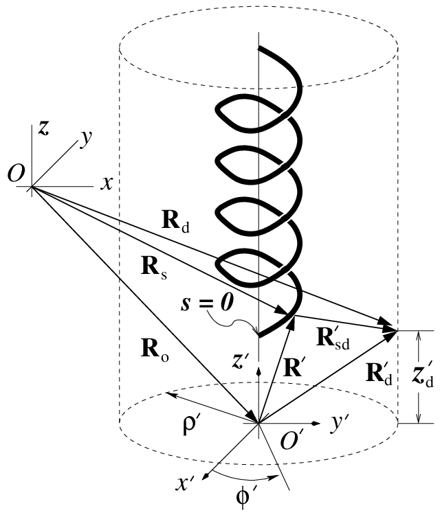
Refer to caption
Figure 17: Position of detector relative to the unprimed origin.

In MKS system of units, where length is measured in meters, mass is measured in kilograms, and time is measured in seconds, the constants g,g, η,\eta, and γ\gamma of Eqs. (4) thru (6) are identified as

g=14​π​εo,η=1,γ=μo4​πg=\frac{1}{4\pi\varepsilon_{\textup{o}}},\quad\eta=1,\quad\gamma=\frac{\mu_{\textup{o}}}{4\pi}

and the constant KK in Eq. (12) gets identified as

K=ω​γ​ηg=ω​μo​εo,K=\omega\sqrt{\frac{\gamma\eta}{g}}=\omega\sqrt{\mu_{\textup{o}}\varepsilon_{\textup{o}}},

where the free space electric permittivity εo\varepsilon_{\textup{o}} and the magnetic permeability μo\mu_{\textup{o}} have the value given by

εo\displaystyle\varepsilon_{\textup{o}} ≈8.854×10⁻¹²​ s4​A2​m−3​kg−1,\displaystyle\approx 8.854\times 10^{-12}\textnormal{ {s}}^{4}\,\textnormal{{A}}^{2}\,\textnormal{{m}}^{-3}\,\textnormal{{kg}}^{-1},
μo\displaystyle\mu_{\textup{o}} =4​π×10−7​ m​kg​s−2​A−2.\displaystyle=4\pi\times 10^{-7}\textnormal{ {m}}\,\textnormal{{kg}}\,\textnormal{{s}}^{-2}\,\textnormal{{A}}^{-2}.

The total electric field and the total magnetic induction part of the electromagnetic wave reaching the surface of an imaginary cylindrical shell, illustrated in Fig. 17, can be summarized as

𝐄total=𝐄P′+𝐄rad,\displaystyle\mathbf{E}_{\textup{total}}=\mathbf{E}_{\textup{P}}^{\prime}+\mathbf{E}_{\textup{rad}}, 𝐁total=𝐁P′+𝐁rad,\displaystyle\mathbf{B}_{\textup{total}}=\mathbf{B}_{\textup{P}}^{\prime}+\mathbf{B}_{\textup{rad}},

where 𝐄P′\mathbf{E}_{\textup{P}}^{\prime} and 𝐁P′\mathbf{B}_{\textup{P}}^{\prime} respectively represent the electric field and the magnetic induction parts of electromagnetic waves other than the radiation from nanohelix reaching the detector. The measure of field amplification, therefore, may be expressed as

EtotalEP=‖𝐄P′+𝐄rad‖‖𝐄P‖,\displaystyle\frac{E_{\textup{total}}}{E_{\textup{P}}}=\frac{\left\|\mathbf{E}_{\textup{P}}^{\prime}+\mathbf{E}_{\textup{rad}}\right\|}{\left\|\mathbf{E}_{\textup{P}}\right\|}, BtotalBP=‖𝐁P′+𝐁rad‖‖𝐁P‖.\displaystyle\frac{B_{\textup{total}}}{B_{\textup{P}}}=\frac{\left\|\mathbf{B}_{\textup{P}}^{\prime}+\mathbf{B}_{\textup{rad}}\right\|}{\left\|\mathbf{B}_{\textup{P}}\right\|}.

In many situations, the magnitudes of 𝐄P′\mathbf{E}_{\textup{P}}^{\prime} and 𝐁P′\mathbf{B}_{\textup{P}}^{\prime} are only minute changes from that of incidence wave, i.e., ‖𝐄P‖≈‖𝐄P′‖\left\|\mathbf{E}_{\textup{P}}\right\|\approx\left\|\mathbf{E}_{\textup{P}}^{\prime}\right\| and ‖𝐁P‖≈‖𝐁P′‖,\left\|\mathbf{B}_{\textup{P}}\right\|\approx\left\|\mathbf{B}_{\textup{P}}^{\prime}\right\|, and the previous expressions can be approximated as

EtotalEP\displaystyle\frac{E_{\textup{total}}}{E_{\textup{P}}} ≈1+‖𝐄rad‖‖𝐄P‖>‖𝐄P+𝐄rad‖‖𝐄P‖,\displaystyle\approx 1+\frac{\left\|\mathbf{E}_{\textup{rad}}\right\|}{\left\|\mathbf{E}_{\textup{P}}\right\|}>\frac{\left\|\mathbf{E}_{\textup{P}}+\mathbf{E}_{\textup{rad}}\right\|}{\left\|\mathbf{E}_{\textup{P}}\right\|}, (132)
BtotalBP\displaystyle\frac{B_{\textup{total}}}{B_{\textup{P}}} ≈1+‖𝐁rad‖‖𝐁P‖>‖𝐁P+𝐁rad‖‖𝐁P‖.\displaystyle\approx 1+\frac{\left\|\mathbf{B}_{\textup{rad}}\right\|}{\left\|\mathbf{B}_{\textup{P}}\right\|}>\frac{\left\|\mathbf{B}_{\textup{P}}+\mathbf{B}_{\textup{rad}}\right\|}{\left\|\mathbf{B}_{\textup{P}}\right\|}. (133)

A successful rectification of ambient electromagnetic wave requires the field amplification criterion defined in Eq. (3),

EtotalEP≫1,\displaystyle\frac{E_{\textup{total}}}{E_{\textup{P}}}\gg 1, BtotalBP≫1,\displaystyle\frac{B_{\textup{total}}}{B_{\textup{P}}}\gg 1,

where the subscripts in the magnitudes of electric field and magnetic induction have been modified from rad to total.\textup{total}. Observing Eqs. (132) and (133), the requirement for a successful rectification of ambient electromagnetic wave is given by

EradEP≫1,\displaystyle\frac{E_{\textup{rad}}}{E_{\textup{P}}}\gg 1, BradBP≫1,\displaystyle\frac{B_{\textup{rad}}}{B_{\textup{P}}}\gg 1,

which is the field amplification criterion defined in Eq. (3).

I am now ready to plot the results. For convenience, the origins of two reference frames, OO and O′,O^{\prime}, were made to coincide each other. This makes xo​1=xo​2=0,x_{\textup{o}1}=x_{\textup{o}2}=0, zd=zd′,z_{\textup{d}}=z_{\textup{d}}^{\prime}, and △​zd=△​zd′.\triangle z_{\textup{d}}=\triangle z_{\textup{d}}^{\prime}. Furthermore, it had been assumed that the helix winding started at zd=zd′=0z_{\textup{d}}=z_{\textup{d}}^{\prime}=0 and the vacuum was assumed for the medium holding both the finite helix and the propagating incidence and radiated electromagnetic waves. That being said, Eqs. (88) and (122) are computed at the surface of cylindrical screen of radius ρ′,\rho^{\prime}, Eq. (131), using Simpson method coded in FORTRAN 90 for numerical integration25 and assuming the following input values,

wavelength​λ=555.016​nm,\textup{wavelength}\,\lambda=555.016\,\textup{nm},
wave number vector: 𝐊(K,0,0)=K𝐱^=2​πλ𝐱^,\textup{wave number vector: }\mathbf{K}\left(K,0,0\right)=K\hat{\mathbf{x}}=\frac{2\pi}{\lambda}\hat{\mathbf{x}},
polarization: 𝐄P(α1=π2,α2=0,α3=π2)=EP𝐲^,\textup{polarization: }\mathbf{E}_{\textup{P}}\left(\alpha_{1}=\frac{\pi}{2},\alpha_{2}=0,\alpha_{3}=\frac{\pi}{2}\right)=E_{\textup{P}}\hat{\mathbf{y}},
radius of helix: a=40nm,\textup{radius of helix: }a=40\,\textup{nm},
pitch of helix: pitch=50nm,\textup{pitch of helix: }\textup{pitch}=50\,\textup{nm},
radius of screen: ρ′=273nm,\textup{radius of screen: }\rho^{\prime}=273\,\textup{nm},
increment along z axis: △zd′=0.0976nm,\textup{increment along z axis: }\triangle z_{\textup{d}}^{\prime}=0.0976\,\textup{nm},
helix conductivity: σ=5×10⁵S,\textup{helix conductivity: }\sigma=5\times 10^{5}\,\textup{S},
fully streched length of helix: l=5um,\textup{fully streched length of helix: }l=5\,\textup{um},
helix winding number: Nw=19.5.\textup{helix winding number: }N_{\textup{w}}=19.5.

The results are illustrated in Figs. 18 thru 21, where the parameter hh in Figs. 18 and 20 represents the height of nanohelix, i.e., h=b​c,h=bc, as illustrated in Fig. 11. The results illustrated in Figs. 19 and 21, therefore, respectively represent slices of Figs. 18 and 20 at helix height indicated by zd.z_{\textup{d}}.

Refer to caption
Figure 18: The ratio Brad/BpB_{\textup{rad}}/B_{\textnormal{p}} measured on the surface of cylindrical screen of radius ρ′=273​nm.\rho^{\prime}=273\,\textup{nm}.
Refer to caption
Figure 19: The ratio Brad/Bp,B_{\textup{rad}}/B_{\textnormal{p}}, which is measured on the surface of cylindrical screen of radius ρ′=273​nm\rho^{\prime}=273\,\textup{nm} and sliced at indicated zd.z_{\textup{d}}.
Refer to caption
Figure 20: The ratio Erad/EpE_{\textup{rad}}/E_{\textnormal{p}} measured on the surface of cylindrical screen of radius ρ′=273​nm.\rho^{\prime}=273\,\textup{nm}.
Refer to caption
Figure 21: The ratio Erad/Ep,E_{\textup{rad}}/E_{\textnormal{p}}, which is measured on the surface of cylindrical screen of radius ρ′=273​nm\rho^{\prime}=273\,\textup{nm} and sliced at indicated zd.z_{\textup{d}}.

For the particular case where the input electromagnetic wave is specified by the wave number vector 𝐊=K​𝐱^\mathbf{K}=K\hat{\mathbf{x}} and 𝐄P=EP​𝐲^,\mathbf{E}_{\textup{P}}=E_{\textup{P}}\hat{\mathbf{y}}, the resulting induced radiation from a single nanohelix is characterized by an electric field part which is distorted in profile. The distortion in electric field profile can be attributed to the local geometrical configuration of the nanohelix, e.g., the winding pitch, etc. At distances far away from nanohelix, such effects arising from the geometrical configuration of nanohelix should be averaged out, resulting in a radiated electric field profile which is symmetrical in shape. To confirm such behavior for the scattered fields at distances far away from scattering nanohelix, Eqs. (88) and (122) were re-computed with only the radius of cylindrical screen changed to ρ′=233.04​um,\rho^{\prime}=233.04\,\textup{um}, which is about thousand times larger than the previous value for the radius, ρ′=273​nm.\rho^{\prime}=273\,\textup{nm}. The results are shown in Figs. 22 and 23 for the ratios involving electric and magnetic fields, respectively. As expected, the profiles for both magnetic induction and electric field portray a symmetry about common axis.

Refer to caption
Figure 22: The ratio Brad/BpB_{\textup{rad}}/B_{\textnormal{p}} measured on the surface of cylindrical screen of radius ρ′=233.04​um.\rho^{\prime}=233.04\,\textup{um}.
Refer to caption
Figure 23: The ratio Erad/EpE_{\textup{rad}}/E_{\textnormal{p}} measured on the surface of cylindrical screen of radius ρ′=233.04​um.\rho^{\prime}=233.04\,\textup{um}.

The proposed energy harvesting device based on nanohelices is actually an array of many pixels, where the term pixel has been adopted from display technology to denote a smaller energy harvesting device unit composing of single nanohelix (or few nanohelices). In such many-body (many-nanohelix) system, contributions arising from interaction with different nanohelices must also be taken into account for a total effect, which is a very challenging task. However, without having to go through such difficult calculations involving many-body effect, one can be sure of the existence of locations where constructive and destructive interference of wavelets occur within the layer containing nanohelices. The “number” wins in energy harvesting device based on nanohelices. Since there are billions of nanohelices in the system, even if only one hundredth of them actually participate in the energy harvesting, the total output power generated would be substantial. And, the demonstrated calculation based on single nanohelix, supports the possibility of harvesting energy utilizing nanohelices. Any calculations involving many-nanohelices effect should be deferred for the optimization stage of the development process.

VI Concluding remarks

The presented energy harvesting device based on nanohelices, in all respects, can be thought of as a miniaturized version of rectifier circuits with transformers found in many electronic systems. The only difference is that rectifier based on nanohelices rectify ambient electromagnetic waves, whereas the conventional rectifiers rectify AC source from the household wall outlet. As with all rectifiers, the rectification condition defined in Eq. (1) must be satisfied before the proposed device can actually convert ambient electromagnetic waves into a useful DC electrical power. The rectification condition can be satisfied if the condition defined in Eq. (3) can be met,

EradEP≫1,\displaystyle\frac{E_{\textup{rad}}}{E_{\textup{P}}}\gg 1, BradBP≫1.\displaystyle\frac{B_{\textup{rad}}}{B_{\textup{P}}}\gg 1.

In this work, by utilizing the secondary radiation process, I have explicitly shown that the condition imposed by Eq. (3) becomes feasible with nanohelices.

VII Acknowledgments

The author acknowledges the support for this work provided by Samsung Electronics, Ltd.

References

  • [1] R. Bailey, “A proposed new concept for a solar-energy converter,” Journal of Engineering for Power, 73 (1972)
  • [2] R. Corkish, M. Green, and T. Puzzer, “Solar energy collection by antennas,” Solar Energy 73 (6), pp. 395-401 (2002).
  • [3] R. Corkish, M. Green, T. Puzzer, and T. Humphrey, “Efficiency of antenna solar collection,” in Proceedings of 3rd World Conference on Photovoltaic Energy Conversion, 2003, 3, pp. 2682-2685.
  • [4] N. Karmakar, P. Weng, and S. Roy, “Development of rectenna for microwave power reception,” in 9th Australian Symposium on Antennas, (Sydney, Australia, 2005).
  • [5] N. Hudak and G. Amatucci, “Small-scale energy harvesting through thermoelectric, vibration, and radio frequency power conversion,” J. Appl. Phys. 103, 101301 (2008).
  • [6] D. Kotter, S. Novack, W. Slafer, and P. Pinhero, “Solar nantenna electromagnetic collectors,” in Proceedings of ES2008, Energy Sustainability 2008, (Jacksonville, Florida, USA, 2008), ES2008-54016.
  • [7] C. Balanis, Antenna Theory. Analysis and Design, 2nd Ed, (John Wiley & Sons, USA, 2005).
  • [8] L. Tsakalakos, J. Lee, C. Korman, S. Leboeuf, A. Ebong, R. Wojnarowski, A. Srivastava, and O. Sulima, “High efficiency inorganic nanorod-enhanced photovoltaic devices,” U.S. Patent 20060207647 (2006).
  • [9] A. Sarychev, D. Genov, A. Wei, and V. Shalaev, “Periodical Arrays of Optical Nanoantennas,” in Proceedings of SPIE 5218 (2003).
  • [10] M. Chen, D. Yuan, J. Liu, and X. Han, “Nanoscale Dipole Antennas Based On Long Carbon Nanotubes,” in Proceedings of the 7th IEEE International Conference on Nanotechnology, (August 2-5, Hong Kong, 2007).
  • [11] D. Zhang, A. Alkhateeb, H. Han, H. Mahmood, D. N. McIlroy, and M. Norton, “Silicon Carbide Nanosprings,” Nano Lett. 3 (7), pp. 983-987 (2003).
  • [12] K. Nakamatsu, M. Nagase, H. Namatsu, and S. Matsui, “Mechanical Characteristics of Diamond-Like-Carbon Nanosprings Fabricated by Focused-Ion-beam Chemical Vapor Deposition,” Jap. J. Appl. Phys. 44 (39), pp. L1228-L1230 (2005).
  • [13] G. Dice, M. Brett, D. Wang, and J. Buriak, “Fabrication and characterization of an electrically variable, nanospring based interferometer,” Appl. Phys. Lett. 90, 253101 (2007).
  • [14] C. Daraio, V. Nesterenko, S. jin, W. Wang, and A. Rao, “Impact response by a foam like forest of coiled carbon nanotubes,” J. Appl. Phys. 100, 064309 (2006).
  • [15] G. Zhang and Y. Zhao, “Mechanical characteristics of nanoscale springs,” J. Appl. Phys. 95 (1), pp. 267-271 (2004).
  • [16] J. Singh, D. Liu, D. Ye, R. Picu, T. Lu, and G. Wang, “Metal-coated Si springs: Nanoelectromechanical actuators,” Appl. Phys. Lett. 84 (18), pp. 3657-3659 (2004).
  • [17] J. Phillips, “Retractable helical antenna,” U.S. Patent 4725845 (1988).
  • [18] H. Nakano, H. Takeda, Y. Kitamura, H. Mimaki, and J. Yamauchi, “Low-Profile Helical Array Antenna fed from a Radial Waveguide,” IEEE Transaction on antenna and propagation, 40 (3), pp. 279-284 (1992).
  • [19] D. Griffiths, Introduction to Electrodynamics, 2nd Ed, Prentice-Hall, NJ, USA (1989).
  • [20] M. Born and E. Wolf, Principle of Optics: Electromagnetic Theory of Propagation, Interference and Diffraction of Light (Cambridge University Press, Cambridge, 1980).
  • [21] S. Cho, “Solar cell using nano-helix,” Korean Patent 10-2008-0079928 (2008).
  • [22] S. Cho, “Solar cell using nano-helix,” Korean Patent 10-2008-0127271 (2008).
  • [23] D. H. Weber, A. Beyer, B. Völkel, A. Gölzhäuser, E. Schlenker, A. Bakin, and A. Waag, “Determination of the specific resistance of individual freestanding ZnO nanowires with the low energy electron point source microscope,” Appl. Phys. Lett. 91, 253126 (2007).
  • [24] H. Davis and A. Snider, Introduction to Vector Analysis, 6th Ed, (McGraw-Hill, USA, 1991).
  • [25] G. Thomas and R. Finney, Calculus and analytic geometry, 7th Ed, (Addison-Wesley, USA, 1988).