跳到论文正文
W Papers独立论文阅读器 arXiv:0901.0764 论文正文 计算阅读时间 · 0%
引用这篇论文根据当前论文元数据生成,正式投稿前建议核对。


License: arXiv.org perpetual non-exclusive license
arXiv:0901.0764v1 [math.NA] 07 Jan 2009

Local Multigrid in 𝐇⁡(𝐜𝐮𝐫𝐥)\mathbf{H}(\mathbf{\operatorname{{\bf curl}}})

Ralf Hiptmair ††thanks: SAM, ETH Zürich, CH-8092 Zürich, hiptmair@sam.math.ethz.ch    Weiying Zheng ††thanks: LSEC, Institute of Computational Mathematics, Academy of Mathematics and System Sciences, Chinese Academy of Sciences, Beijing, 100080, People’s Republic of China. This author was supported in part by China NSF under the grant 10401040 (zwy@lsec.cc.ac.cn).
Research Report 2007-03, Seminar for Applied Mathematics, ETH Zürich
Abstract

We consider 𝑯⁡(𝐜𝐮𝐫𝐥,Ω)\boldsymbol{H}(\operatorname{{\bf curl}},{\Omega})-elliptic variational problems on bounded Lipschitz polyhedra and their finite element Galerkin discretization by means of lowest order edge elements. We assume that the underlying tetrahedral mesh has been created by successive local mesh refinement, either by local uniform refinement with hanging nodes or bisection refinement. In this setting we develop a convergence theory for the the so-called local multigrid correction scheme with hybrid smoothing. We establish that its convergence rate is uniform with respect to the number of refinement steps. The proof relies on corresponding results for local multigrid in a H1​(Ω)H^{1}({\Omega})-context along with local discrete Helmholtz-type decompositions of the edge element space.

keywords
Edge elements, local multigrid, stable multilevel splittings, subspace correction theory, regular decompositions of 𝑯⁡(𝐜𝐮𝐫𝐥,Ω)\boldsymbol{H}(\operatorname{{\bf curl}},{\Omega}), Helmholtz-type decompositions, local mesh refinement
AMS
65N30, 65N55, 78A25
𝑯⁡(𝐜𝐮𝐫𝐥,Ω)\boldsymbol{H}(\operatorname{{\bf curl}},{\Omega}) : Sobolev space of square integrable vector fields on Ω⊂ℝ3\Omega\subset\mathbb{R}^{3} with square integrable 𝐜𝐮𝐫𝐥\operatorname{{\bf curl}}
𝑯ΓD​(𝐜𝐮𝐫𝐥,Ω)\boldsymbol{H}_{\Gamma_{D}}(\operatorname{{\bf curl}},{\Omega}) : vector fields in 𝑯⁡(𝐜𝐮𝐫𝐥,Ω)\boldsymbol{H}(\operatorname{{\bf curl}},{\Omega}) with vanishing tangential components on ΓD⊂∂Ω\Gamma_{D}\subset\partial\Omega
ℳ{\cal M}, 𝒯{\cal T} : tetrahedral finite element meshes, may contain hanging nodes
𝒩⁡(ℳ){\cal N}({\cal M}) : set of vertices (nodes) of a mesh ℳ{\cal M}
ℰ⁡(ℳ){\cal E}({\cal M}) : set of edges of a mesh ℳ{\cal M}
ρK,ρℳ\rho_{K},\rho_{{\cal M}} : shape regularity measures
hh : – local meshwidth function for a finite element mesh – (as subscript) tag for finite element functions
𝐔⁡(ℳ){\mathbf{U}}({\cal M}) : lowest order edge element space on ℳ{\cal M}
𝐛E{\mathbf{b}}_{E} : nodal basis function of 𝐔⁡(ℳ){\mathbf{U}}({\cal M}) associated with edge EE
V⁡(ℳ)V({\cal M}) : space of continuous piecewise linear functions on ℳ{\cal M}
V2​(ℳ)V_{2}({\cal M}) : quadratic Lagrangian finite element space on ℳ{\cal M}
V~2​(ℳ)\widetilde{V}_{2}({\cal M}) : quadratic surplus space, see (26)
b𝒑b_{{\boldsymbol{p}}} : nodal basis function of V⁡(ℳ)V({\cal M}) (“tent function”) associated with vertex 𝒑{\boldsymbol{p}}
𝔅X​(ℳ)\mathfrak{B}_{X}({\cal M}) : set of nodal basis functions for finite element space XX on mesh ℳ{\cal M}
𝚷h\boldsymbol{\Pi}_{h} : nodal edge interpolation operator onto 𝐔⁡(ℳ){\mathbf{U}}({\cal M}), see (2.1)
ℐh{\cal I}_{h} : vertex based piecewise linar interpolation onto V⁡(ℳ)V({\cal M})
ℙp\mathbb{P}_{p} : space of 3-variate polynomials of total degree ≤p\leq p
𝐔¯​(ℳ)\overline{{\mathbf{U}}}({\cal M}), V¯​(ℳ)\overline{V}({\cal M}) : finite element spaces oblivious of zero boundary conditions
≺\prec : nesting of finite element meshes
ℓ⁡(K)\ell(K) : level of element KK in hierarchy of refined meshes
ωl\omega_{l} : refinement zone, see (39)
Σl\Sigma_{l} : refinement strip, see (106)
𝔅Vl\mathfrak{B}_{V}^{l}, 𝔅𝐔l\mathfrak{B}_{{\mathbf{U}}}^{l} : sets of basis functions supported inside refinement zones, see (47)
𝖰h\mathsf{Q}_{h} : quasi-interpolation operator, Def. 12
Table 1: Important notation used in this paper

1 Introduction

On a polyhedron Ω⊂ℝ3\Omega{\subset\mathbb{R}^{3}}, scaled such that diam⁡(Ω)=1\operatorname{diam}(\Omega)=1, we consider the variational problem: seek 𝐮∈𝑯ΓD​(𝐜𝐮𝐫𝐥,Ω){\mathbf{u}}\in\boldsymbol{H}_{\Gamma_{D}}(\operatorname{{\bf curl}},{\Omega}) such that

(1) (𝐜𝐮𝐫𝐥⁡𝐮,𝐜𝐮𝐫𝐥⁡𝐯)L2​(Ω)+(𝐮,𝐯)L2​(Ω)⏟=:𝖺⁡(𝐮,𝐯)=(𝐟,𝐯)L2​(Ω)∀𝐯∈𝑯ΓD(𝐜𝐮𝐫𝐥,Ω).\displaystyle\underbrace{\left({\operatorname{{\bf curl}}{\mathbf{u}}},{\operatorname{{\bf curl}}{\mathbf{v}}}\right)_{L^{2}({\Omega})}+\left({{\mathbf{u}}},{{\mathbf{v}}}\right)_{L^{2}({\Omega})}}_{=:\mathsf{a}({\mathbf{u}},{\mathbf{v}})}=\left({{\mathbf{f}}},{{\mathbf{v}}}\right)_{L^{2}({\Omega})}\quad\forall{\mathbf{v}}\in\boldsymbol{H}_{\Gamma_{D}}(\operatorname{{\bf curl}},{\Omega})\;.

For the Hilbert space of square integrable vector fields with square integrable 𝐜𝐮𝐫𝐥\operatorname{{\bf curl}} and vanishing tangential components on ΓD\Gamma_{D} we use the symbol 𝑯ΓD​(𝐜𝐮𝐫𝐥,Ω)\boldsymbol{H}_{\Gamma_{D}}(\operatorname{{\bf curl}},{\Omega}), see [24, Ch. 1] for details. The source term 𝐟{\mathbf{f}} in (1) is a vector field in (L2​(Ω))3(L^{2}({\Omega}))^{3}. The left hand side of (1) agrees with the inner product of 𝑯ΓD​(𝐜𝐮𝐫𝐥,Ω)\boldsymbol{H}_{\Gamma_{D}}(\operatorname{{\bf curl}},{\Omega}) and will be abbreviated by 𝖺⁡(𝐮,𝐯)\mathsf{a}({\mathbf{u}},{\mathbf{v}}) (“energy inner product”).

Further, ΓD\Gamma_{D} denotes the part of the boundary ∂Ω\partial\Omega on which homogeneous Dirichlet boundary conditions in the form of vanishing tangential traces of 𝐮{\mathbf{u}} are imposed. The geometry of the Dirichlet boundary part ΓD\Gamma_{D} is supposed to be simple in the following sense: for each connected component Γi\Gamma_{i} of ΓD\Gamma_{D} we can find an open Lipschitz domain Ωi⊂ℝ3\Omega_{i}\subset\mathbb{R}^{3} such that

(2) Ω¯i∩Ω¯=Γi,Ωi∩Ω=∅,\displaystyle\overline{\Omega}_{i}\cap\overline{\Omega}=\Gamma_{i}\;,\quad\Omega_{i}\cap\Omega=\emptyset\;,

and Ωi\Omega_{i} and Ωj\Omega_{j} have positive distance for i≠ji\not=j. Further, the interior of Ω¯∪Ω1¯∪Ω2¯​…\overline{\Omega}\cup\overline{\Omega_{1}}\cup\overline{\Omega_{2}}\dots is expected to be a Lipschitz-domain, too (see Fig. 11). This is not a severe restriction, because variational problems related to (1) usually arise in quasi-static electromagnetic modelling, where simple geometries are common. Of course, ΓD=∅\Gamma_{D}=\emptyset is admitted.

Lowest order 𝑯ΓD​(𝐜𝐮𝐫𝐥,Ω)\boldsymbol{H}_{\Gamma_{D}}(\operatorname{{\bf curl}},{\Omega})-conforming edge elements are widely used for the finite element Galerkin discretization of variational problems like (1). Then, for a solution 𝐮∈(H1​(Ω))3{\mathbf{u}}\in(H^{1}({\Omega}))^{3} with 𝐜𝐮𝐫𝐥⁡𝐮∈(H1​(Ω))3\operatorname{{\bf curl}}{\mathbf{u}}\in(H^{1}({\Omega}))^{3} we can expect the optimal asymptotic convergence rate

(3) ‖𝐮−𝐮h‖𝑯⁡(𝐜𝐮𝐫𝐥,Ω)≤CNh−1/3,\displaystyle\left\|{{\mathbf{u}}-{\mathbf{u}}_{h}}\right\|_{\boldsymbol{H}(\operatorname{{\bf curl}},{\Omega})}\leq CN_{h}^{-1/3}\;,

on families of finite element meshes arising from global refinement. Here, 𝐮h{\mathbf{u}}_{h} is the finite element solution, NhN_{h} the dimension of the finite element space, and C>0C>0 does not depend on NhN_{h}. However, often 𝐮{\mathbf{u}} will fail to possess the required regularity due to singularities arising at edges/corners of ∂Ω\partial\Omega and material interfaces [23, 22]. Fortunately, it seems to be possible to retain (3) by the use of adaptive local mesh refinement based on a posteriori error estimates, see [55, 10] for theory in H1H^{1}-setting, [17, 7] for numerical evidence in the case of edge element discretization, and [52, 34, 8] for related theoretical investigations.

We also need ways to compute the asymptotically optimal finite element solution with optimal computational effort, that is, with a number of operations proportional to NhN_{h}. This can only be achieved by means of iterative solvers, whose convergence remains fast regardless of the depth of refinement. Multigrid methods are the most prominent class of iterative solvers that achieve this goal. By now, geometric multigrid methods for discrete 𝑯⁡(𝐜𝐮𝐫𝐥,Ω)\boldsymbol{H}(\operatorname{{\bf curl}},{\Omega})-elliptic variational problems like (1) have become well established [29, 54, 58, 20]. Their asymptotic theory on sequencies of regularly refined meshes has also matured [2, 25, 29, 31, 51]. It confirms asymptotic optimality: the speed of convergence is uniformly fast regardless of the number of refinement levels involved. In addition, the costs of one step of the iteration scale linearly with the number of unknowns.

Yet, the latter property is lost when the standard multigrid correction scheme is applied to meshes generated by pronounced local refinement. Optimal computational costs can only be maintained, if one adopts the local multigrid policy, which was pioneered by A. Brandt et al. in [5], see also [41]. Crudely speaking, its gist is to confine relaxations to “new” degrees of freedom located in zones where refinement has changed the mesh. Thus an exponential increase of computational costs with the number of refinement levels can be avoided: the total costs of a V-cycle remain proportional to the number of unknowns. An algorithm blending the local multigrid idea with the geometric multigrid correction scheme of [29] is described in [54]. On the other hand, a proof of uniform asymptotic convergence has remained elusive so far. It is the objective of this paper to provide it, see Theorem 11.

We recall the key insight that (1) is one member of a family of variational problems. Its kin is obtained by replacing 𝐜𝐮𝐫𝐥\operatorname{{\bf curl}} with 𝐠𝐫𝐚𝐝\operatorname{{\bf grad}} or div\operatorname{div}, respectively. All these differential operators turn out to be incarnations of the fundamental exterior derivative of differential geometry, cf. [29, Sect. 2]. They are closely connected in the deRham complex [3] and, thus, it is hardly surprising that results about the related HΓD1​(Ω)H_{\Gamma_{D}}^{1}({\Omega})-elliptic variational problem, which seeks u∈HΓD1​(Ω)u\in H_{\Gamma_{D}}^{1}({\Omega}) such that

(4) (𝐠𝐫𝐚𝐝⁡u,𝐠𝐫𝐚𝐝⁡v)L2​(Ω)+(u,v)L2​(Ω)=(f,v)L2​(Ω)∀v∈HΓD1​(Ω),\displaystyle\left({\operatorname{{\bf grad}}u},{\operatorname{{\bf grad}}v}\right)_{L^{2}({\Omega})}+\left({u},{v}\right)_{L^{2}({\Omega})}=\left({f},{v}\right)_{L^{2}({\Omega})}\quad\forall\,v\in H_{\Gamma_{D}}^{1}({\Omega})\;,

prove instrumental in the multigrid analysis for discretized versions of (1). Here HΓD1​(Ω)H_{\Gamma_{D}}^{1}({\Omega}) is the subspace of H1​(Ω)H^{1}({\Omega}) whose functions have vanishing traces on ΓD\Gamma_{D}.

Thus, when tackling (1), we take the cue from the local multigrid theory for (4) discretized by means of linear continuous finite elements. This theory has been developed in various settings, cf. [5, 11, 15, 14, 62]. In [1] local refinement with hanging nodes is treated. Recently, H. Wu and Z. Chen [60] proved the uniform convergence of local multigrid V-cycles on adaptively refined meshes in two dimensions. Their mesh refinements are controlled by a posteriori error estimators and carried out according to the “newest vertex bisection” strategy introduced, independently, in [40, 6].

As in the case of global multigrid, the essential new aspect of local multigrid theory for (1) compared to (4) is the need to deal with the kernel of the 𝐜𝐮𝐫𝐥\operatorname{{\bf curl}}-operator, cf. [29, Sect. 3]. In this context, the availability of discrete scalar potential representations for irrotational edge element vector fields is pivotal. Therefore, we devote the entire Sect. 2 to the discussion of edge elements and their relationship with conventional Lagrangian finite elements. Meshes with hanging nodes will receive particular attention. Next, in Sect. 3 we present details about local mesh refinement, because some parts of the proofs rest on the subtleties of how elements are split. The following Sect. 4 introduces the local multigrid method from the abstract perspective of successive subspace correction.

The proof of uniform convergence (Theorem 11) is tackled in Sects. 5 and 6, which form the core of the article. In particular, the investigation of the stability of the local multilevel splitting requires several steps, the first of which addresses the issue for the bilinear form from (4) and linear finite elements. These results are already available in the literature, but are re-derived to make the presentation self-contained. This also applies to the continuous and discrete Helmholtz-type decompositions covered in Sect. 5.3. Many developments are rather technical and to aid the reader important notations are listed in Table 1. Eventually, in Sect. 7, we report two numerical experiments to show the competitive performance of the local multigrid method and the relevance of the convergence theory.

Remark 1.

In this article we forgo generality and do not discuss the more general bi-linear form

(5) 𝖺⁡(𝐮,𝐯):=(α​𝐜𝐮𝐫𝐥⁡𝐮,𝐜𝐮𝐫𝐥⁡𝐯)L2​(Ω)+(β​𝐮,𝐯)L2​(Ω),∀𝐮,𝐯∈𝑯ΓD​(𝐜𝐮𝐫𝐥,Ω),\displaystyle\mathsf{a}({\mathbf{u}},{\mathbf{v}}):=\left({\alpha\operatorname{{\bf curl}}{\mathbf{u}}},{\operatorname{{\bf curl}}{\mathbf{v}}}\right)_{L^{2}({\Omega})}+\left({\beta{\mathbf{u}}},{{\mathbf{v}}}\right)_{L^{2}({\Omega})}\;,\quad\forall{\mathbf{u}},{\mathbf{v}}\in\boldsymbol{H}_{\Gamma_{D}}(\operatorname{{\bf curl}},{\Omega})\;,

with uniformly positive coefficient functions α,β∈L∞​(Ω)\alpha,\beta\in L^{\infty}(\Omega). We do this partly for the sake of lucidity and partly, because the current theory cannot provide estimates that are robust with respect to large variations of α\alpha and β\beta, cf. [33]. We refer to [63] for further information and references.

2 Finite element spaces

Whenever we refer to a finite element mesh in this article, we have in mind a tetrahedral triangulation of Ω\Omega, see [19, Ch. 3]. In certain settings, it may feature hanging nodes, that is, the face of one tetrahedron can coincide with the union of faces of other tetrahedra. Further, the mesh is supposed to resolve the Dirichlet boundary in the sense that ΓD\Gamma_{D} is the union of faces of tetrahedra. The symbol ℳ{\cal M} with optional subscripts is reserved for finite element meshes and the sets of their elements alike.

We write h∈L∞​(Ω)h\in L^{\infty}({\Omega}) for the piecewise constant function, which assumes value hK:=diam⁡(K)h_{K}:=\operatorname{diam}(K) in each element K∈ℳK\in{\cal M}. The ratio of diam⁡(K)\operatorname{diam}(K) to the radius of the largest ball contained in KK is called the shape regularity measure ρK\rho_{K} [19, Ch. 3, §3.1]. The shape regularity measure ρℳ\rho_{{\cal M}} of ℳ{\cal M} is the maximum of all ρK\rho_{K}, K∈ℳK\in{\cal M}.

2.1 Conforming meshes

Provisionally, we consider only finite element meshes ℳ{\cal M} that are conforming, that is, each face of a tetrahedron is either contained in ∂Ω\partial\Omega or a face of another tetrahedron, see [19, Ch. 2, § 2.2]. In particular, this rules out hanging nodes. Following [43, 12], we introduce the space of lowest order 𝑯ΓD​(𝐜𝐮𝐫𝐥,Ω)\boldsymbol{H}_{\Gamma_{D}}(\operatorname{{\bf curl}},{\Omega})-conforming edge finite elements, also known as Whitney-1-forms [59],

(6) 𝐔(ℳ):={𝐯h∈𝑯ΓD(𝐜𝐮𝐫𝐥,Ω):∀K∈ℳ:∃𝒂,𝒃∈ℝ3:\displaystyle{\mathbf{U}}({\cal M}):=\{{\mathbf{v}}_{h}\in\boldsymbol{H}_{\Gamma_{D}}(\operatorname{{\bf curl}},{\Omega}):\;\forall\,K\in{\cal M}:\exists\,{\boldsymbol{a}},{\boldsymbol{b}}\in\mathbb{R}^{3}:
(7) 𝐯h(𝒙)=𝒂+𝒃×𝒙,𝒙∈K}.\displaystyle{\mathbf{v}}_{h}({\boldsymbol{x}})={\boldsymbol{a}}+{\boldsymbol{b}}\times{\boldsymbol{x}},\;{\boldsymbol{x}}\in K\}\;.

For a detailed derivation and description please consult [30, Sect. 3] or the monographs [42, 13]. Notice that 𝐜𝐮𝐫𝐥⁡𝐔⁡(ℳ)\operatorname{{\bf curl}}{\mathbf{U}}({\cal M}) is a space of piecewise constant vector fields. We also remark that appropriate global degrees of freedom (d.o.f.) for 𝐔⁡(ℳ){\mathbf{U}}({\cal M}) are given by

{𝐔⁡(ℳ)↦ℝ𝐯h↦∫E𝐯h⋅ds→,E∈ℰ⁡(ℳ),\displaystyle\left\{\begin{array}[c]{rcl}{\mathbf{U}}({\cal M})&\mapsto&\mathbb{R}\\ {\mathbf{v}}_{h}&\mapsto&\int\nolimits_{E}{\mathbf{v}}_{h}\cdot\mathrm{d}\vec{s}\end{array}\right.\quad,\quad E\in{\cal E}({\cal M})\;,

where ℰ⁡(ℳ){\cal E}({\cal M}) is the set of edges of ℳ{\cal M} not contained in ΓD\Gamma_{D}. We write 𝔅𝐔​(ℳ)\mathfrak{B}_{{\mathbf{U}}}({\cal M}) for the nodal basis of 𝐔⁡(ℳ){\mathbf{U}}({\cal M}) dual to the global d.o.f. (2.1). Basis functions are associated with active edges. Hence, we can write 𝔅𝐔​(ℳ)={𝐛E}E∈ℰ⁡(ℳ)\mathfrak{B}_{{\mathbf{U}}}({\cal M})=\{{\mathbf{b}}_{E}\}_{E\in{\cal E}({\cal M})}. The support of the basis function 𝐛E{\mathbf{b}}_{E} is the union of tetrahedra sharing the edge EE. We recall the simple formula for local shape functions

(10) 𝐛E|K=λi𝐠𝐫𝐚𝐝λj−λj𝐠𝐫𝐚𝐝λiE=[𝒂i,𝒂j]⊂K¯\displaystyle{{\mathbf{b}}_{E}}_{|K}=\lambda_{i}\operatorname{{\bf grad}}\lambda_{j}-\lambda_{j}\operatorname{{\bf grad}}\lambda_{i}\quad E=[{\boldsymbol{a}}_{i},{\boldsymbol{a}}_{j}]\subset\overline{K}

for any tetrahedron K∈ℳK\in{\cal M} with vertices 𝒂i{\boldsymbol{a}}_{i}, i=1,2,3,4i=1,2,3,4, and associated barycentric coordinate functions λi\lambda_{i}.

The edge element space 𝐔⁡(ℳ){\mathbf{U}}({\cal M}) with basis 𝔅𝐔​(ℳ)\mathfrak{B}_{{\mathbf{U}}}({\cal M}) is perfectly suited for the finite element Galerkin discretization of (1). The discrete problem based on 𝐔⁡(ℳ){\mathbf{U}}({\cal M}) reads: seek 𝐮h∈𝐔⁡(ℳ){\mathbf{u}}_{h}\in{\mathbf{U}}({\cal M}) such that

(11) (𝐜𝐮𝐫𝐥⁡𝐮h,𝐜𝐮𝐫𝐥⁡𝐯h)L2​(Ω)+(𝐮h,𝐯h)L2​(Ω)=(𝐟,𝐯h)L2​(Ω)∀𝐯h∈𝐔⁡(ℳ).\displaystyle\left({\operatorname{{\bf curl}}{\mathbf{u}}_{h}},{\operatorname{{\bf curl}}{\mathbf{v}}_{h}}\right)_{L^{2}({\Omega})}+\left({{\mathbf{u}}_{h}},{{\mathbf{v}}_{h}}\right)_{L^{2}({\Omega})}=\left({{\mathbf{f}}},{{\mathbf{v}}_{h}}\right)_{L^{2}({\Omega})}\quad\forall{\mathbf{v}}_{h}\in{\mathbf{U}}({\cal M})\;.

The properties of 𝐔⁡(ℳ){\mathbf{U}}({\cal M}) will be key to constructing and analyzing the local multigrid method for the large sparse linear system of equations resulting from (11). Next, we collect important facts.

The basis 𝔅𝐔​(ℳ)\mathfrak{B}_{{\mathbf{U}}}({\cal M}) enjoys uniform L2L^{2}-stability, meaning the existence of a constant11 1 The symbol CC will stand for generic positive constants throughout this article. Its value may vary between different occurrences. We will always specify on which quantities these constants may depend. C=C⁡(ρℳ)>0C=C(\rho_{{\cal M}})>0 such that for all 𝐯h=∑E∈ℰ⁡(ℳ)αE​𝐛E∈𝐔⁡(ℳ){\mathbf{v}}_{h}=\sum\limits_{E\in{\cal E}({\cal M})}\alpha_{E}{\mathbf{b}}_{E}\in{\mathbf{U}}({\cal M}), αE∈ℝ\alpha_{E}\in\mathbb{R},

(12) C−1​‖𝐯h‖L2​(Ω)2≤∑E∈ℰ⁡(ℳ)αE2​‖𝐛E‖L2​(Ω)2≤C​‖𝐯h‖L2​(Ω)2.\displaystyle C^{-1}\left\|{{\mathbf{v}}_{h}}\right\|_{L^{2}({\Omega})}^{2}\leq\sum\limits_{E\in{\cal E}({\cal M})}\alpha_{E}^{2}\left\|{{\mathbf{b}}_{E}}\right\|_{L^{2}({\Omega})}^{2}\leq C\left\|{{\mathbf{v}}_{h}}\right\|_{L^{2}({\Omega})}^{2}\;.

The global d.o.f. induce a nodal edge interpolation operator

𝚷h:{dom⁡(𝚷h)⊂𝑯ΓD​(𝐜𝐮𝐫𝐥,Ω)↦𝐔⁡(ℳ)𝐯↦∑E∈ℰ⁡(ℳ)(∫E𝐯⋅ds→)⋅𝐛E.\displaystyle\boldsymbol{\Pi}_{h}:\left\{\begin{array}[c]{rcl}\operatorname{dom}(\boldsymbol{\Pi}_{h})\subset\boldsymbol{H}_{\Gamma_{D}}(\operatorname{{\bf curl}},{\Omega})&\mapsto&{\mathbf{U}}({\cal M})\\ {\mathbf{v}}&\mapsto&\sum\limits_{E\in{\cal E}({\cal M})}\Bigl(\int\nolimits_{E}{\mathbf{v}}\cdot\mathrm{d}\vec{s}\Bigr)\cdot{\mathbf{b}}_{E}\;.\end{array}\right.

Obviously, 𝚷h\boldsymbol{\Pi}_{h} provides a local projection, but it turns out to be unbounded even on (H1​(Ω))3(H^{1}({\Omega}))^{3}. Only for vector fields with discrete rotation the following interpolation error estimate is available, see [30, Lemma 4.6]:

Lemma 2.

The interpolation operator 𝚷h\boldsymbol{\Pi}_{h} is bounded on {𝚿∈(H1​(Ω))3,𝐜𝐮𝐫𝐥⁡𝚿∈𝐜𝐮𝐫𝐥⁡𝐔⁡(ℳ)}⊂(H1​(Ω))3\{\boldsymbol{\Psi}\in(H^{1}({\Omega}))^{3},\,\operatorname{{\bf curl}}\boldsymbol{\Psi}\in\operatorname{{\bf curl}}{\mathbf{U}}({\cal M})\}{\subset(H^{1}({\Omega}))^{3}}, and for any conforming mesh there is C=C⁡(ρℳ)>0C=C(\rho_{{\cal M}})>0 such that

‖h−1​(I​d−𝚷h)​𝚿‖L2​(Ω)≤C​|𝚿|H1​(Ω)∀𝚿∈(H1​(Ω))3,𝐜𝐮𝐫𝐥⁡𝚿∈𝐜𝐮𝐫𝐥⁡𝐔⁡(ℳ).\displaystyle\left\|{h^{-1}(Id-\boldsymbol{\Pi}_{h})\boldsymbol{\Psi}}\right\|_{L^{2}({\Omega})}\leq C{\left|{\boldsymbol{\Psi}}\right|}_{H^{1}({\Omega})}\quad\forall\boldsymbol{\Psi}\in(H^{1}({\Omega}))^{3},\;\operatorname{{\bf curl}}\boldsymbol{\Psi}\in\operatorname{{\bf curl}}{\mathbf{U}}({\cal M})\;.

If Ω\Omega is homeomorphic to a ball, then 𝐠𝐫𝐚𝐝⁡H1​(Ω)=𝑯⁡(𝐜𝐮𝐫𝐥⁡0,Ω):={𝐯∈𝑯⁡(𝐜𝐮𝐫𝐥,Ω),𝐜𝐮𝐫𝐥⁡𝐯=0}\operatorname{{\bf grad}}H^{1}({\Omega})=\boldsymbol{H}(\operatorname{{\bf curl}}0,{\Omega}):=\{{\mathbf{v}}\in\boldsymbol{H}(\operatorname{{\bf curl}},{\Omega}),\,\operatorname{{\bf curl}}{\mathbf{v}}=0\}, that is, H1​(Ω)H^{1}({\Omega}) provides scalar potentials for 𝑯⁡(𝐜𝐮𝐫𝐥,Ω)\boldsymbol{H}(\operatorname{{\bf curl}},{\Omega}). To state a discrete analogue of this relationship we need the Lagrangian finite element space of piecewise linear continuous functions on ℳ{\cal M}

(15) V(ℳ):={uh∈HΓD1(Ω):uh|K∈ℙ1(K)∀K∈ℳ},\displaystyle V({\cal M}):=\{u_{h}\in H_{\Gamma_{D}}^{1}({\Omega}):\;{u_{h}}_{|K}\in\mathbb{P}_{1}(K)\;\forall K\in{\cal M}\}\;,

where ℙp​(K)\mathbb{P}_{p}(K) is the space of 3-variate polynomials of degree ≤p\leq p on KK. The global degrees of freedom for V⁡(ℳ)V({\cal M}) boil down to point evaluations at the vertices of ℳ{\cal M} away from Γ¯D\overline{\Gamma}_{D} (set 𝒩⁡(ℳ){\cal N}({\cal M})). The dual basis of “tent functions” will be denoted by 𝔅V​(ℳ)={b𝒑}𝒑∈𝒩⁡(ℳ)\mathfrak{B}_{V}({\cal M})={\{b_{{\boldsymbol{p}}}\}}_{{\boldsymbol{p}}\in{\cal N}({\cal M})}. Its unconditional L2L^{2}-stability is well known: with a universal constant C>0C>0 we have for all uh=∑𝒑∈𝒩⁡(ℳ)α𝒑​b𝒑∈V⁡(ℳ)u_{h}=\sum\limits_{{\boldsymbol{p}}\in{\cal N}({\cal M})}\alpha_{{\boldsymbol{p}}}b_{{\boldsymbol{p}}}\in V({\cal M}), α𝒑∈ℝ\alpha_{{\boldsymbol{p}}}\in\mathbb{R},

(16) C−1​‖uh‖L2​(Ω)2≤∑𝒑∈𝒩⁡(ℳ)α𝒑2​‖b𝒑‖L2​(Ω)2≤C​‖uh‖L2​(Ω)2.\displaystyle C^{-1}\left\|{u_{h}}\right\|_{L^{2}({\Omega})}^{2}\leq\sum\limits_{{\boldsymbol{p}}\in{\cal N}({\cal M})}\alpha_{{\boldsymbol{p}}}^{2}\left\|{b_{{\boldsymbol{p}}}}\right\|_{L^{2}({\Omega})}^{2}\leq C\left\|{u_{h}}\right\|_{L^{2}({\Omega})}^{2}\;.

For the nodal interpolation operator related to 𝔅V\mathfrak{B}_{V} we write ℐh:dom⁡(ℐh)⊂HΓD1​(Ω)↦V⁡(ℳ){\cal I}_{h}:\operatorname{dom}({\cal I}_{h})\subset H_{\Gamma_{D}}^{1}({\Omega})\mapsto V({\cal M}). Recall the standard estimate for linear interpolation on conforming meshes (i.e., no hanging nodes allowed), [19, Thm. 3.2.1], that asserts the existence of C=C⁡(k,ρℳ)>0C=C(k,\rho_{{\cal M}})>0 such that

(17) ‖hk−2​(I​d−ℐh)​u‖Hk​(Ω)≤C​|u|H2​(Ω)∀u∈H2​(Ω)∩HΓD1​(Ω),k∈{0,1}.\displaystyle{\left\|{h^{k-2}(Id-{\cal I}_{h})u}\right\|}_{H^{k}({\Omega})}\leq C{\left|{u}\right|}_{H^{2}({\Omega})}\quad\forall u\in H^{2}({\Omega})\cap H_{\Gamma_{D}}^{1}({\Omega}),\;k\in\{0,1\}\;.

Obviously, 𝐠𝐫𝐚𝐝⁡V⁡(ℳ)⊂𝐔⁡(ℳ)\operatorname{{\bf grad}}V({\cal M})\subset{\mathbf{U}}({\cal M}), and immediate from Stokes theorem is the crucial commuting diagram property

(18) 𝚷h∘𝐠𝐫𝐚𝐝=𝐠𝐫𝐚𝐝∘ℐhon dom(ℐh).\displaystyle\boldsymbol{\Pi}_{h}\circ\operatorname{{\bf grad}}=\operatorname{{\bf grad}}\circ{\cal I}_{h}\quad\text{on }\operatorname{dom}({\cal I}_{h})\;.

This enables us to give an elementary proof of Lemma 2.

of Lemma 2.

Pick one K∈ℳK\in{\cal M} and, without loss of generality, assume 0∈K0\in K. Then define the lifting operator, cf. the “Koszul lifting” [3, Sect. 3.2],

(19) 𝐰↦ℒ⁡𝐰,ℒ⁡𝐰⁡(𝒙):=13​𝐰​(𝒙)×𝒙,𝒙∈K.\displaystyle{\mathbf{w}}\mapsto\operatorname{{\cal L}}{\mathbf{w}}\;,\quad\operatorname{{\cal L}}{\mathbf{w}}({\boldsymbol{x}}):=\tfrac{1}{3}{\mathbf{w}}({\boldsymbol{x}})\times{\boldsymbol{x}}\;,\quad{\boldsymbol{x}}\in K\;.

Elementary calculations reveal that for any constant vectorfield 𝐰∈(𝒫0​(K))3{\mathbf{w}}\in({\cal P}_{0}(K))^{3}

(20) 𝐜𝐮𝐫𝐥⁡ℒ⁡𝐰=𝐰,\displaystyle\operatorname{{\bf curl}}\operatorname{{\cal L}}{\mathbf{w}}={\mathbf{w}}\;,
(21) ‖ℒ⁡𝐰‖L2​(K)≤hK​‖𝐰‖L2​(K),\displaystyle\left\|{\operatorname{{\cal L}}{\mathbf{w}}}\right\|_{L^{2}({K})}\leq h_{K}\left\|{{\mathbf{w}}}\right\|_{L^{2}({K})}\;,
(22) ℒ⁡𝐰∈𝐔⁡(K).\displaystyle\operatorname{{\cal L}}{\mathbf{w}}\in{\mathbf{U}}(K)\;.

The continuity (21) permits us to extend ℒ\operatorname{{\cal L}} to (L2​(K))3(L^{2}({K}))^{3}.

Given 𝚿∈(H1​(K))3\boldsymbol{\Psi}\in(H^{1}({K}))^{3} with 𝐜𝐮𝐫𝐥⁡𝚿≡const3\operatorname{{\bf curl}}\boldsymbol{\Psi}\equiv\mathrm{const}^{3}, by (22) we know ℒ⁡𝐜𝐮𝐫𝐥⁡𝚿∈(𝒫1​(K))3\operatorname{{\cal L}}\operatorname{{\bf curl}}\boldsymbol{\Psi}\in({\cal P}_{1}(K))^{3}. Thus, an inverse inequality leads to

(23) |ℒ⁡𝐜𝐮𝐫𝐥⁡𝚿|H1​(K)≤C​hK−1​‖ℒ⁡𝐜𝐮𝐫𝐥⁡𝚿‖L2​(K)​≤(21)​C​‖𝐜𝐮𝐫𝐥⁡𝚿‖L2​(K),\displaystyle{\left|{\operatorname{{\cal L}}\operatorname{{\bf curl}}\boldsymbol{\Psi}}\right|}_{H^{1}({K})}\leq Ch_{K}^{-1}\left\|{\operatorname{{\cal L}}\operatorname{{\bf curl}}\boldsymbol{\Psi}}\right\|_{L^{2}({K})}\overset{\text{\eqref{eq:femLP2}}}{\leq}C\left\|{\operatorname{{\bf curl}}\boldsymbol{\Psi}}\right\|_{L^{2}({K})}\;,

with C=C⁡(ρK)>0C=C(\rho_{K})>0. Next, (20) implies

(24) 𝐜𝐮𝐫𝐥(𝚿−ℒ𝐜𝐮𝐫𝐥𝚿)=0⇒∃p∈H1(K):𝚿−ℒ𝐜𝐮𝐫𝐥𝚿=𝐠𝐫𝐚𝐝p.\displaystyle\operatorname{{\bf curl}}(\boldsymbol{\Psi}-\operatorname{{\cal L}}\operatorname{{\bf curl}}\boldsymbol{\Psi})=0\quad\Rightarrow\quad\exists p\in H^{1}({K}):\quad\boldsymbol{\Psi}-\operatorname{{\cal L}}\operatorname{{\bf curl}}\boldsymbol{\Psi}=\operatorname{{\bf grad}}p\;.

From (23) we conclude that p∈H2​(K)p\in H^{2}({K}) and |p|H2​(K)≤C​|𝚿|H1​(K){\left|{p}\right|}_{H^{2}({K})}\leq C{\left|{\boldsymbol{\Psi}}\right|}_{H^{1}({K})}. Moreover, thanks to the commuting diagram property we have

(25) 𝚿−𝚷h𝚿=ℒ⁡𝐜𝐮𝐫𝐥⁡𝚿−𝚷h​ℒ⁡𝐜𝐮𝐫𝐥⁡𝚿⏟=0by (22)+𝐠𝐫𝐚𝐝(p−ℐhp),\displaystyle\boldsymbol{\Psi}-\boldsymbol{\Pi}_{h}\boldsymbol{\Psi}=\underbrace{\operatorname{{\cal L}}\operatorname{{\bf curl}}\boldsymbol{\Psi}-\boldsymbol{\Pi}_{h}\operatorname{{\cal L}}\operatorname{{\bf curl}}\boldsymbol{\Psi}}_{=0\;\text{by \eqref{eq:femLP3}}}+\operatorname{{\bf grad}}(p-{\cal I}_{h}p)\;,

which means, by the standard estimate (17) for linear interpolation on KK,

‖𝚿−𝚷h​𝚿‖L2​(K)=|p−ℐh​p|H1​(K)≤C​hK​|p|H2​(K)≤C​hK​|𝚿|H1​(K).\displaystyle\left\|{\boldsymbol{\Psi}-\boldsymbol{\Pi}_{h}\boldsymbol{\Psi}}\right\|_{L^{2}({K})}={\left|{p-{\cal I}_{h}p}\right|}_{H^{1}({K})}\leq Ch_{K}{\left|{p}\right|}_{H^{2}({K})}\leq Ch_{K}{\left|{\boldsymbol{\Psi}}\right|}_{H^{1}({K})}\;.

Summation over all elements finishes the proof. ∎

As theoretical tools we need “higher order” counterparts of the above finite element spaces. We recall the quadratic Lagrangian finite element space

(26) V2(ℳ):={uh∈HΓD1(Ω):uh|K∈ℙ2(K)∀K∈ℳ},\displaystyle V_{2}({\cal M}):=\{u_{h}\in H_{\Gamma_{D}}^{1}({\Omega}):\;{u_{h}}_{|K}\in\mathbb{P}_{2}(K)\;\forall K\in{\cal M}\}\;,

and its subspace of quadratic surpluses

(27) V~2​(ℳ):={uh∈V2​(ℳ):ℐh​uh=0}.\displaystyle\widetilde{V}_{2}({\cal M}):=\{u_{h}\in V_{2}({\cal M}):\;{\cal I}_{h}u_{h}=0\}\;.

This implies a direct splitting

(28) V2​(ℳ)=V⁡(ℳ)⊕V~2​(ℳ),\displaystyle V_{2}({\cal M})=V({\cal M})\oplus\widetilde{V}_{2}({\cal M})\;,

which is unconditionally H1H^{1}-stable: there is a C=C⁡(ρℳ)>0C=C(\rho_{{\cal M}})>0 such that

(29) C−1​|uh|H1​(Ω)2≤|(I​d−ℐh)​uh|H1​(Ω)2+|ℐh​uh|H1​(Ω)2≤C​|uh|H1​(Ω)2,\displaystyle C^{-1}{\left|{{u}_{h}}\right|}_{H^{1}({\Omega})}^{2}\leq{\left|{(Id-{\cal I}_{h}){u}_{h}}\right|}_{H^{1}({\Omega})}^{2}+{\left|{{\cal I}_{h}{u}_{h}}\right|}_{H^{1}({\Omega})}^{2}\leq C{\left|{{u}_{h}}\right|}_{H^{1}({\Omega})}^{2}\;,

for all uh∈V2​(ℳ){u}_{h}\in{V}_{2}({\cal M}).

Next, we examine the space (V⁡(ℳ))3(V({\cal M}))^{3} of continuous piecewise linear vector fields that vanish on ΓD\Gamma_{D}. Standard affine equivalence techniques for edge elements, see [30, Sect. 3.6], confirm

(30) ∃C=C⁡(ρℳ)>0:‖𝚷h​𝚿h‖L2​(Ω)≤C​‖𝚿h‖L2​(Ω)∀𝚿h∈(V⁡(ℳ))3.\displaystyle\exists C=C(\rho_{{\cal M}})>0:\quad\left\|{\boldsymbol{\Pi}_{h}\boldsymbol{\Psi}_{h}}\right\|_{L^{2}({\Omega})}\leq C\left\|{\boldsymbol{\Psi}_{h}}\right\|_{L^{2}({\Omega})}\quad\forall\boldsymbol{\Psi}_{h}\in(V({\cal M}))^{3}\;.
Lemma 3.

For all 𝚿h∈(V⁡(ℳ))3\boldsymbol{\Psi}_{h}\in(V({\cal M}))^{3} we can find v~h∈V~2​(ℳ)\widetilde{v}_{h}\in\widetilde{V}_{2}({\cal M}) such that

𝚿h=𝚷h​𝚿h+𝐠𝐫𝐚𝐝⁡v~h,\displaystyle\boldsymbol{\Psi}_{h}=\mathbf{\Pi}_{h}\boldsymbol{\Psi}_{h}+\operatorname{{\bf grad}}\widetilde{v}_{h}\;,

and, with C=C⁡(ρℳ)>0C=C(\rho_{{\cal M}})>0,

C−1​‖𝚿h‖L2​(Ω)2≤‖𝚷h​𝚿h‖L2​(Ω)2+‖𝐠𝐫𝐚𝐝⁡v~h‖L2​(Ω)2≤C​‖𝚿h‖L2​(Ω)2.\displaystyle C^{-1}\left\|{\boldsymbol{\Psi}_{h}}\right\|_{L^{2}({\Omega})}^{2}\leq\left\|{\mathbf{\Pi}_{h}\boldsymbol{\Psi}_{h}}\right\|_{L^{2}({\Omega})}^{2}+\left\|{\operatorname{{\bf grad}}\widetilde{v}_{h}}\right\|_{L^{2}({\Omega})}^{2}\leq C\left\|{\boldsymbol{\Psi}_{h}}\right\|_{L^{2}({\Omega})}^{2}\;.

For the proof we rely on a very useful insight, which relieves us from all worries concerning the topology of Ω\Omega:

Lemma 4.

If 𝐯∈𝐇ΓD​(𝐜𝐮𝐫𝐥⁡0,Ω){\mathbf{v}}\in\boldsymbol{H}_{\Gamma_{D}}(\operatorname{{\bf curl}}0,{\Omega}) and 𝚷h​𝐯=0\boldsymbol{\Pi}_{h}{\mathbf{v}}=0, then 𝐯∈𝐠𝐫𝐚𝐝⁡HΓD1​(Ω){\mathbf{v}}\in\operatorname{{\bf grad}}H_{\Gamma_{D}}^{1}({\Omega}).

Proof.

Since the mesh covers Ω\Omega, the relative homology group H1​(Ω,ΓD)H_{1}(\Omega;\Gamma_{D}) is generated by a set of edge paths. By definition (2.1) of the d.o.f. of 𝐔⁡(ℳ){\mathbf{U}}({\cal M}), the path integrals of 𝐯{\mathbf{v}} along all these paths vanish. As an irrotational vector field with vanishing circulation along a complete set of ΓD\Gamma_{D}-relative fundamental cycles, 𝐯{\mathbf{v}} must be a gradient. ∎

of Lemma 3.

Given 𝚿h∈(V⁡(ℳ))3\boldsymbol{\Psi}_{h}\in(V({\cal M}))^{3}, we decompose it according to

(31) 𝚿h=𝚷h𝚿h+(I​d−𝚷h)​𝚿h⏟=:𝐠𝐫𝐚𝐝⁡v~h.\displaystyle\boldsymbol{\Psi}_{h}=\boldsymbol{\Pi}_{h}\boldsymbol{\Psi}_{h}+\underbrace{(Id-\boldsymbol{\Pi}_{h})\boldsymbol{\Psi}_{h}}_{=:\operatorname{{\bf grad}}\widetilde{v}_{h}}\;.

Note that 𝐜𝐮𝐫𝐥⁡(I​d−𝚷h)​𝚿h\operatorname{{\bf curl}}(Id-\boldsymbol{\Pi}_{h})\boldsymbol{\Psi}_{h} is piecewise constant with vanishing flux through all triangular faces of ℳ{\cal M}. Then Stokes’ theorem teaches that 𝐜𝐮𝐫𝐥⁡(I​d−𝚷h)​𝚿h=0\operatorname{{\bf curl}}(Id-\boldsymbol{\Pi}_{h})\boldsymbol{\Psi}_{h}=0.

By the projector property of 𝚷h\boldsymbol{\Pi}_{h}, (I​d−𝚷h)​𝚿h(Id-\boldsymbol{\Pi}_{h})\boldsymbol{\Psi}_{h} satisfies the assumptions of Lemma 4. Taking into account that, moreover, the field is piecewise linear, it is clear that (I​d−𝚷h)​𝚿h=𝐠𝐫𝐚𝐝⁡ψ(Id-\boldsymbol{\Pi}_{h})\boldsymbol{\Psi}_{h}=\operatorname{{\bf grad}}\psi with ψ∈V2​(ℳ)\psi\in V_{2}({\cal M}). Along an arbitrary edge path γ\gamma in ℳ{\cal M} we have ∫γ(I​d−𝚷h)​𝚿h⋅𝑑s→=0\int\nolimits_{\gamma}(Id-\boldsymbol{\Pi}_{h})\boldsymbol{\Psi}_{h}\cdot\mathrm{d}\vec{s}=0 so that ψ\psi attains the same value (w.l.o.g. =0=0) on all vertices of ℳ{\cal M}. The stability of the splitting is a consequence of (30). ∎

By definition, the spaces 𝐔⁡(ℳ){\mathbf{U}}({\cal M}) and V⁡(ℳ)V({\cal M}) accommodate the homogeneous boundary conditions on ΓD\Gamma_{D}. Later, we will also need finite element spaces oblivious of boundary conditions, that is, for the case ΓD=∅\Gamma_{D}=\emptyset. These will be tagged by a bar on top, e.g., 𝐔¯​(ℳ)\overline{{\mathbf{U}}}({\cal M}), V¯​(ℳ)\overline{V}({\cal M}), etc. The same convention will be employed for notions and operators associated with finite element spaces: if they refer to the particular case ΓD=∅\Gamma_{D}=\emptyset, they will be endowed with an overbar, e.g. 𝚷¯h\overline{\boldsymbol{\Pi}}_{h}, ℐ¯h\overline{{\cal I}}_{h}, 𝔅¯𝐔​(ℳ)\overline{\mathfrak{B}}_{{\mathbf{U}}}({\cal M}), 𝒩¯​(ℳ)\overline{{\cal N}}({\cal M}), etc.

2.2 Meshes with hanging nodes

Now, general tetrahedral meshes with hanging nodes are admitted. We simply retain the definitions (15) and (26) of the spaces V⁡(ℳ)V({\cal M}) and V2​(ℳ)V_{2}({\cal M}) of continuous finite element functions. Degrees of freedom for V⁡(ℳ)V({\cal M}) are point evaluations at active vertices of ℳ{\cal M}. A vertex is called active, if it is not located in the interior of an edge/face of ℳ{\cal M} or on ΓD\Gamma_{D}. A 2D22 2 For ease of visualization, we will often elucidate geometric concepts in two-dimensional settings. Their underlying ideas are the same in 2D and 3D. illustration is given in Fig. 1.

Refer to caption

ℳ0{\cal M}_{0}

Refer to caption

ℳ1{\cal M}_{1}

Refer to caption

ℳ2{\cal M}_{2}

Refer to caption

ℳ3{\cal M}_{3}

Fig. 1: Active vertices (∙\bullet) of 2D triangular meshes with hanging nodes, Ω=]0,1[2\Omega=]0,1[^{2}, ΓD=∂Ω\Gamma_{D}=\partial\Omega. In ℳ1,ℳ2,ℳ3{\cal M}_{1},{\cal M}_{2},{\cal M}_{3} active edges are marked with green arrows.

The values of a finite element function at the remaining (“slave”) vertices are determined by recursive affine interpolation. A dual nodal basis 𝔅V​(ℳ)\mathfrak{B}_{V}({\cal M}) and corresponding interpolation operator ℐh{\cal I}_{h} can be defined as above.

In principle, the definition (6) of the edge element space could be retained on non-conforming meshes, as well. Yet, for this choice an edge interpolation operator 𝚷h\boldsymbol{\Pi}_{h} that satisfies the commuting diagram property (18) is not available. Thus, we construct basis functions directly and rely on the notion of active edges, see Fig. 1.

Definition 5.

An edge of ℳ{\cal M} is active, if it is an edge of some K∈ℳK\in{\cal M}, not contained in ΓD\Gamma_{D}, and connects two vertices that are either active or located on ΓD\Gamma_{D}.

We keep the symbol ℰ⁡(ℳ){\cal E}({\cal M}) to designate the set of active edges of ℳ{\cal M}. To each E∈ℰ⁡(ℳ)E\in{\cal E}({\cal M}) we associate a basis function 𝐛E{\mathbf{b}}_{E}, which, locally on the tetrahedra of ℳ{\cal M}, is a polynomial of the form (7). In order to fix this basis function completely, it suffices to speficify its path integrals (2.1) along all edges of ℳ{\cal M}. In the spirit of duality, we demand

(32) ∫F𝐛E⋅𝑑s→={1, if ​F=E,0, if ​F∈ℰ⁡(ℳ)∖{E}.\displaystyle\int\nolimits_{F}{\mathbf{b}}_{E}\cdot\mathrm{d}\vec{s}=\begin{cases}1&\text{, if }F=E\;,\\ 0&\text{, if }F\in{\cal E}({\cal M})\setminus\{E\}\;.\end{cases}

For the non-active (“slave”) edges of ℳ{\cal M} the path integrals of 𝐛E{\mathbf{b}}_{E} (subsequently called “weights”) are chosen to fit (18), keeping in mind that 𝔅𝐔​(ℳ):={𝐛E}E∈ℰ⁡(ℳ)\mathfrak{B}_{{\mathbf{U}}}({\cal M}):=\{{\mathbf{b}}_{E}\}_{E\in{\cal E}({\cal M})}, and that the d.o.f. and 𝚷h\boldsymbol{\Pi}_{h} are still defined according to (2.1) and (2.1), respectively. Ultimately, we set 𝐔⁡(ℳ):=Span⁡{𝔅𝐔​(ℳ)}{\mathbf{U}}({\cal M}):=\operatorname{Span}\left\{{\mathfrak{B}_{{\mathbf{U}}}({\cal M})}\right\}.

Let us explain the policy for setting the weights in the case of the subdivided tetrahedron of Fig. 2 with hanging nodes at the midpoints of edges, which will turn out to be the only relevant situation, cf. Sect. 5.3. Weights have to be assigned to the “small edges” of the refined tetrahedron, some of which will be active, and some of which will have “slave” status, see the caption of Fig. 2.

We write the direction vectors of slave edges as linear combinations of active edges, for instance,

𝒒1−𝒑3\displaystyle{\boldsymbol{q}}_{1}-{\boldsymbol{p}}_{3} =12​(𝒑4−𝒑3),\displaystyle=\tfrac{1}{2}({\boldsymbol{p}}_{4}-{\boldsymbol{p}}_{3})\;,
𝒒1−𝒒2\displaystyle{\boldsymbol{q}}_{1}-{\boldsymbol{q}}_{2} =12​(𝒑4+𝒑3)−12​(𝒑2+𝒑3)=12​(𝒑4−𝒑2),\displaystyle=\tfrac{1}{2}({\boldsymbol{p}}_{4}+{\boldsymbol{p}}_{3})-\tfrac{1}{2}({\boldsymbol{p}}_{2}+{\boldsymbol{p}}_{3})=\tfrac{1}{2}({\boldsymbol{p}}_{4}-{\boldsymbol{p}}_{2})\;,
𝒑5−𝒒4\displaystyle{\boldsymbol{p}}_{5}-{\boldsymbol{q}}_{4} =𝒑5−12​(𝒑1+𝒑3)=𝒑5−𝒑1+12​(𝒑1−𝒑3),\displaystyle={\boldsymbol{p}}_{5}-\tfrac{1}{2}({\boldsymbol{p}}_{1}+{\boldsymbol{p}}_{3})={\boldsymbol{p}}_{5}-{\boldsymbol{p}}_{1}+\tfrac{1}{2}({\boldsymbol{p}}_{1}-{\boldsymbol{p}}_{3})\;,
𝒒4−𝒒3\displaystyle{\boldsymbol{q}}_{4}-{\boldsymbol{q}}_{3} =12​(𝒑1+𝒑3)−12​(𝒑4+𝒑2)=12​(𝒑1−𝒑2)+12​(𝒑3−𝒑4).\displaystyle=\tfrac{1}{2}({\boldsymbol{p}}_{1}+{\boldsymbol{p}}_{3})-\tfrac{1}{2}({\boldsymbol{p}}_{4}+{\boldsymbol{p}}_{2})=\tfrac{1}{2}({\boldsymbol{p}}_{1}-{\boldsymbol{p}}_{2})+\tfrac{1}{2}({\boldsymbol{p}}_{3}-{\boldsymbol{p}}_{4})\;.

In a sence, we express slave edges as “linear combinations” of active edges. In a different context, this policy is explained in more detail in [26].

Refer to caption
Fig. 2: Subdivided tetrahedron, active vertices (∙\bullet) 𝒑1,…,𝒑6{\boldsymbol{p}}_{1},\ldots,{\boldsymbol{p}}_{6}, slave vertices (∘\circ) 𝒒1,…,𝒒4{\boldsymbol{q}}_{1},\ldots,{\boldsymbol{q}}_{4}, active edges [𝒑1,𝒑5][{\boldsymbol{p}}_{1},{\boldsymbol{p}}_{5}], [𝒑1,𝒑6][{\boldsymbol{p}}_{1},{\boldsymbol{p}}_{6}], [𝒑4,𝒑5][{\boldsymbol{p}}_{4},{\boldsymbol{p}}_{5}], [𝒑2,𝒑6][{\boldsymbol{p}}_{2},{\boldsymbol{p}}_{6}], [𝒑2,𝒑3][{\boldsymbol{p}}_{2},{\boldsymbol{p}}_{3}], [𝒑2,𝒑4][{\boldsymbol{p}}_{2},{\boldsymbol{p}}_{4}], [𝒑3,𝒑4][{\boldsymbol{p}}_{3},{\boldsymbol{p}}_{4}], [𝒑5,𝒑6][{\boldsymbol{p}}_{5},{\boldsymbol{p}}_{6}], [𝒑1,𝒑3][{\boldsymbol{p}}_{1},{\boldsymbol{p}}_{3}], slave edges [𝒑1,𝒒4][{\boldsymbol{p}}_{1},{\boldsymbol{q}}_{4}], [𝒒4,𝒑3][{\boldsymbol{q}}_{4},{\boldsymbol{p}}_{3}], [𝒑2,𝒒2][{\boldsymbol{p}}_{2},{\boldsymbol{q}}_{2}], [𝒒2,𝒑3][{\boldsymbol{q}}_{2},{\boldsymbol{p}}_{3}], [𝒑3,𝒒1][{\boldsymbol{p}}_{3},{\boldsymbol{q}}_{1}], [𝒒1,𝒑4][{\boldsymbol{q}}_{1},{\boldsymbol{p}}_{4}], [𝒑6,𝒒4][{\boldsymbol{p}}_{6},{\boldsymbol{q}}_{4}], [𝒒2,𝒒4][{\boldsymbol{q}}_{2},{\boldsymbol{q}}_{4}], [𝒑6,𝒒2][{\boldsymbol{p}}_{6},{\boldsymbol{q}}_{2}], [𝒒1,𝒒2][{\boldsymbol{q}}_{1},{\boldsymbol{q}}_{2}], [𝒒2,𝒒3][{\boldsymbol{q}}_{2},{\boldsymbol{q}}_{3}], [𝒒1,𝒒3][{\boldsymbol{q}}_{1},{\boldsymbol{q}}_{3}], [𝒒1,𝒑5][{\boldsymbol{q}}_{1},{\boldsymbol{p}}_{5}], [𝒒3,𝒑5][{\boldsymbol{q}}_{3},{\boldsymbol{p}}_{5}], [𝒒4,𝒑5][{\boldsymbol{q}}_{4},{\boldsymbol{p}}_{5}]

The coefficients in the combinations tell us the weights. For example, for the active edge E=[𝒑3,𝒑4]E=[{\boldsymbol{p}}_{3},{\boldsymbol{p}}_{4}] in Fig. 2 they are given in Table 2. Using these weights and the formula (10), 𝐛E{\mathbf{b}}_{E} can be assembled on the tetrahedron by imposing (see Table 2 for notations)

∫S𝐛E⋅𝑑s→={wSfor any contributing slave edge ​S,0for all other (slave) edges.,S∈{“small edges”}.\displaystyle\int\nolimits_{S}{\mathbf{b}}_{E}\cdot\mathrm{d}\vec{s}=\begin{cases}w_{S}&\text{for any contributing slave edge }S\;,\\ 0&\text{for all other (slave) edges.}\end{cases}\;,\quad S\in\{\text{``small edges''}\}\;.
Slave edge SS [𝒒1,𝐩4][{\boldsymbol{q}}_{1},{\mathbf{p}}_{4}] [𝒑3,𝒒1][{\boldsymbol{p}}_{3},{\boldsymbol{q}}_{1}] [𝒒2,𝒒3][{\boldsymbol{q}}_{2},{\boldsymbol{q}}_{3}] [𝒒4,𝒑5][{\boldsymbol{q}}_{4},{\boldsymbol{p}}_{5}] [𝒒3,𝒒4][{\boldsymbol{q}}_{3},{\boldsymbol{q}}_{4}]
weight wSw_{S} 12\frac{1}{2} 12\frac{1}{2} 12\frac{1}{2} 12\frac{1}{2} −12-\frac{1}{2}
Table 2: Weights for slave edges in Fig. 2 relative to active edge E=[𝒑3,𝒑4]E=[{\boldsymbol{p}}_{3},{\boldsymbol{p}}_{4}]. Only slave edges with non-zero weights are listed.

Firstly, the procedure for the selection of weight guarantees that 𝐠𝐫𝐚𝐝⁡V⁡(ℳ)⊂𝐔⁡(ℳ)\operatorname{{\bf grad}}V({\cal M})\subset{\mathbf{U}}({\cal M}). For illustration, we single out the gradient 𝐰h{\mathbf{w}}_{h} of the nodal basis function belonging to vertex 𝒑5{\boldsymbol{p}}_{5} in Fig. 2. Its path integral equals 11 along the (oriented) edges [𝒑1,𝒑5],[𝒑3,𝒑5],[𝒑6,𝒑5],[𝒒4,𝒑5],[𝒒3,𝒑5],[𝒒1,𝒑5][{\boldsymbol{p}}_{1},{\boldsymbol{p}}_{5}],[{\boldsymbol{p}}_{3},{\boldsymbol{p}}_{5}],[{\boldsymbol{p}}_{6},{\boldsymbol{p}}_{5}],[{\boldsymbol{q}}_{4},{\boldsymbol{p}}_{5}],[{\boldsymbol{q}}_{3},{\boldsymbol{p}}_{5}],[{\boldsymbol{q}}_{1},{\boldsymbol{p}}_{5}], and vanishes on all other edges. Hence we expect

(33) 𝐰h=𝐛[𝒑1,𝒑5]+𝐛[𝒑3,𝒑5]+𝐛[𝒑6,𝒑5].\displaystyle{\mathbf{w}}_{h}={\mathbf{b}}_{[{\boldsymbol{p}}_{1},{\boldsymbol{p}}_{5}]}+{\mathbf{b}}_{[{\boldsymbol{p}}_{3},{\boldsymbol{p}}_{5}]}+{\mathbf{b}}_{[{\boldsymbol{p}}_{6},{\boldsymbol{p}}_{5}]}\;.

This can be verified through showing equality of path integrals along slave edges. We take a close look at the slave edge [𝒒4,𝒑5][{\boldsymbol{q}}_{4},{\boldsymbol{p}}_{5}]. By construction the basis functions belonging to active edges satisfy

∫[𝒒4,𝒑5]𝐛[𝒑1,𝒑5]⋅𝑑s→=1,∫[𝒒4,𝒑5]𝐛[𝒑5,𝒑4]⋅𝑑s→=0,∫[𝒒4,𝒑5]𝐛[𝒑3,𝒑4]⋅𝑑s→=0,\displaystyle\int\limits_{[{\boldsymbol{q}}_{4},{\boldsymbol{p}}_{5}]}{\mathbf{b}}_{[{\boldsymbol{p}}_{1},{\boldsymbol{p}}_{5}]}\cdot\mathrm{d}\vec{s}=1\;,\int\limits_{[{\boldsymbol{q}}_{4},{\boldsymbol{p}}_{5}]}{\mathbf{b}}_{[{\boldsymbol{p}}_{5},{\boldsymbol{p}}_{4}]}\cdot\mathrm{d}\vec{s}=0\;,\int\limits_{[{\boldsymbol{q}}_{4},{\boldsymbol{p}}_{5}]}{\mathbf{b}}_{[{\boldsymbol{p}}_{3},{\boldsymbol{p}}_{4}]}\cdot\mathrm{d}\vec{s}=0\;,
∫[𝒒4,𝒑5]𝐛[𝒑1,𝒑3]⋅𝑑s→=−12,∫[𝒒4,𝒑5]𝐛[𝒑1,𝒑6]⋅𝑑s→=0​∫[𝒒4,𝒑5]𝐛[𝒑2,𝒑6]⋅𝑑s→=0,\displaystyle\int\limits_{[{\boldsymbol{q}}_{4},{\boldsymbol{p}}_{5}]}{\mathbf{b}}_{[{\boldsymbol{p}}_{1},{\boldsymbol{p}}_{3}]}\cdot\mathrm{d}\vec{s}=-\tfrac{1}{2}\;,\int\limits_{[{\boldsymbol{q}}_{4},{\boldsymbol{p}}_{5}]}{\mathbf{b}}_{[{\boldsymbol{p}}_{1},{\boldsymbol{p}}_{6}]}\cdot\mathrm{d}\vec{s}=0\;\int\limits_{[{\boldsymbol{q}}_{4},{\boldsymbol{p}}_{5}]}{\mathbf{b}}_{[{\boldsymbol{p}}_{2},{\boldsymbol{p}}_{6}]}\cdot\mathrm{d}\vec{s}=0\;,
∫[𝒒4,𝒑5]𝐛[𝒑2,𝒑3]⋅𝑑s→=0.\displaystyle\int\limits_{[{\boldsymbol{q}}_{4},{\boldsymbol{p}}_{5}]}{\mathbf{b}}_{[{\boldsymbol{p}}_{2},{\boldsymbol{p}}_{3}]}\cdot\mathrm{d}\vec{s}=0\;.

Then, evidently,

1=∫[𝒒4,𝒑5]𝐰h⋅ds→=∫[𝒒4,𝒑5]𝐛[𝒑1,𝒑5]⋅ds→+∫[𝒒4,𝒑5]𝐛[𝒑3,𝒑5]⋅ds→+∫[𝒒4,𝒑5]𝐛[𝒑6,𝒑5]⋅ds→=1+0+0.1=\int\limits_{[{\boldsymbol{q}}_{4},{\boldsymbol{p}}_{5}]}{\mathbf{w}}_{h}\cdot\mathrm{d}\vec{s}\\ =\int\limits_{[{\boldsymbol{q}}_{4},{\boldsymbol{p}}_{5}]}{\mathbf{b}}_{[{\boldsymbol{p}}_{1},{\boldsymbol{p}}_{5}]}\cdot\mathrm{d}\vec{s}+\int\limits_{[{\boldsymbol{q}}_{4},{\boldsymbol{p}}_{5}]}{\mathbf{b}}_{[{\boldsymbol{p}}_{3},{\boldsymbol{p}}_{5}]}\cdot\mathrm{d}\vec{s}+\int\limits_{[{\boldsymbol{q}}_{4},{\boldsymbol{p}}_{5}]}{\mathbf{b}}_{[{\boldsymbol{p}}_{6},{\boldsymbol{p}}_{5}]}\cdot\mathrm{d}\vec{s}=1+0+0\;.

The same considerations apply to all other slave edges and (33) is established. Secondly, the construction ensures the commuting diagram property (18): again appealing to Fig. 2 we find, for example,

∫[𝒒3,𝒒4]𝐠𝐫𝐚𝐝⁡ℐh​u⋅ds→=ℐh​u​(𝒒4)−ℐh​u​(𝒒3)=12​(u⁡(𝒑4)+u⁡(𝒑2))−12​(u⁡(𝒑1)+u⁡(𝒑3))=12​∫[𝒑3,𝒑4]𝐠𝐫𝐚𝐝⁡u⋅ds→+12​∫[𝒑1,𝒑2]𝐠𝐫𝐚𝐝⁡u⋅ds→=12​∫[𝒑3,𝒑4]𝐠𝐫𝐚𝐝⁡u⋅ds→+14​∫[𝒑1,𝒑6]𝐠𝐫𝐚𝐝⁡u⋅ds→+14​∫[𝒑6,𝒑2]𝐠𝐫𝐚𝐝⁡u⋅ds→.\int\limits_{[{\boldsymbol{q}}_{3},{\boldsymbol{q}}_{4}]}\operatorname{{\bf grad}}{\cal I}_{h}u\cdot\mathrm{d}\vec{s}={\cal I}_{h}u({\boldsymbol{q}}_{4})-{\cal I}_{h}u({\boldsymbol{q}}_{3})=\\ \tfrac{1}{2}(u({\boldsymbol{p}}_{4})+u({\boldsymbol{p}}_{2}))-\tfrac{1}{2}(u({\boldsymbol{p}}_{1})+u({\boldsymbol{p}}_{3}))=\tfrac{1}{2}\int\limits_{[{\boldsymbol{p}}_{3},{\boldsymbol{p}}_{4}]}\operatorname{{\bf grad}}u\cdot\mathrm{d}\vec{s}+\tfrac{1}{2}\int\limits_{[{\boldsymbol{p}}_{1},{\boldsymbol{p}}_{2}]}\operatorname{{\bf grad}}u\cdot\mathrm{d}\vec{s}=\\ \tfrac{1}{2}\int\limits_{[{\boldsymbol{p}}_{3},{\boldsymbol{p}}_{4}]}\operatorname{{\bf grad}}u\cdot\mathrm{d}\vec{s}+\tfrac{1}{4}\int\limits_{[{\boldsymbol{p}}_{1},{\boldsymbol{p}}_{6}]}\operatorname{{\bf grad}}u\cdot\mathrm{d}\vec{s}+\tfrac{1}{4}\int\limits_{[{\boldsymbol{p}}_{6},{\boldsymbol{p}}_{2}]}\operatorname{{\bf grad}}u\cdot\mathrm{d}\vec{s}\;.

In words, combining the path integrals of 𝐠𝐫𝐚𝐝⁡u\operatorname{{\bf grad}}u along active edges with the relative weights of the slave edge [𝒒3,𝒒4][{\boldsymbol{q}}_{3},{\boldsymbol{q}}_{4}] yields the same result as evaluating the path integral of the gradient of the interpolant ℐh​u{\cal I}_{h}u along [𝒒3,𝒒4][{\boldsymbol{q}}_{3},{\boldsymbol{q}}_{4}].

The definitions (26) and (27) also carry over to meshes with hanging nodes. This remains true for the splitting asserted in Lemma 2.2. However, though the algebraic relationships like (18) remain valid, the estimates and norm equivalences of the previous section do not hold for general families of meshes with hanging nodes. This entails restrictions on the location of hanging nodes, whose discussion will be postponed until Sect. 3.2, cf. Assumption 6.1.

Remark 6.

Our presentation is confined to tetrahedral meshes and lowest order edge elements for the sake of simplicity. Extension of all results to hexahedral meshes and higher order edge elements is possible, but will be technical and tedious.

3 Local mesh refinement

We study the case where the actual finite element mesh ℳh{\cal M}_{h} of Ω\Omega has been created by successive local refinement of a relatively uniform initial mesh ℳ0{\cal M}_{0}. Concerning ℳh{\cal M}_{h} and ℳ0{\cal M}_{0} the following asumptions will be made:

  1. 1.

    Given ℳ0{\cal M}_{0} and ℳh{\cal M}_{h} we can construct a virtual refinement hierarchy of L+1L+1 nested33 3 two finite element meshes ℳ{\cal M} and 𝒯{\cal T} are nested, ℳ≺𝒯{\cal M}\prec{\cal T}, if every element of ℳ{\cal M} is the union of elements of 𝒯{\cal T}. tetrahedral meshes, L∈ℕL\in\mathbb{N}:

    (34) ℳ0≺ℳ1≺ℳ2≺⋯≺ℳL=ℳh.\displaystyle{\cal M}_{0}\;\prec\;{\cal M}_{1}\;\prec\;{\cal M}_{2}\;\prec\;\cdots\;\prec{\cal M}_{L}={\cal M}_{h}\;.

    Please note that the virtual refinement hierarchy may be different from the actual sequence of meshes spawned during adaptive refinement44 4 For the local multigrid algorithm examined in this article the implementation must provide access to the virtual refinement hierarchy. This entails suitable bookkeeping data structures, which are available in the ALBERTA package used for the numerical experiments in Sect. 7.

  2. 2.

    Inductively, we assign to each tetrahedron K∈ℳlK\in{\cal M}_{l} a level ℓ⁡(K)∈ℕ0\ell(K)\in\mathbb{N}_{0} by counting the number of subdivisions it took to generate it from an element of ℳ0{\cal M}_{0}.

  3. 3.

    For all 0≤l<L0\leq l<L the mesh ℳl+1{\cal M}_{l+1} is created by subdividing some or all of the tetrahedra in {K∈ℳl:ℓ⁡(K)=l}\{K\in{\cal M}_{l}:\,\ell(K)=l\}.

  4. 4.

    The shape regularity measures of the meshes ℳl{\cal M}_{l} are uniformly bounded independently of LL.

Refinement may be local, but it must be regular in the following sense, cf. [46, Sect. 4.2.2] and [60]: we can find a second sequence of nested tetrahedral meshes of Ω\Omega

(35) ℳ0=ℳ^0≺ℳ^1≺ℳ^2≺⋯≺ℳ^L.\displaystyle{\cal M}_{0}=\widehat{{\cal M}}_{0}\;\prec\;\widehat{{\cal M}}_{1}\;\prec\;\widehat{{\cal M}}_{2}\;\prec\;\cdots\;\prec\widehat{{\cal M}}_{L}\;.

that satisfies

  1. 1.

    ℳl≺ℳ^l{\cal M}_{l}\prec\widehat{{\cal M}}_{l} and {K∈ℳl:ℓ⁡(K)=l}⊂ℳ^l\{K\in{\cal M}_{l}:\,\ell(K)=l\}\subset\widehat{{\cal M}}_{l}, l=0,…,Ll=0,\ldots,L,

  2. 2.

    that the shape regularity measure ρℳ^l\rho_{\widehat{{\cal M}}_{l}} is bounded independently of ll,

  3. 3.

    and that there exist two constants C>0C>0 and 0<θ<10<\theta<1 independent of ll and LL such that

    (36) C−1​θl≤hK≤C​θl∀K∈ℳ^l,0≤l≤L.\displaystyle C^{-1}\theta^{l}\leq h_{K}\leq C\theta^{l}\quad\forall K\in\widehat{{\cal M}}_{l}\;,\quad 0\leq l\leq L\;.

    This means that the family {ℳ^l}l{\{\widehat{{\cal M}}_{l}\}}_{l} is quasi-uniform. Hence, it makes sense to refer to a mesh width hl:=max⁡{hK,K∈ℳ^l}h_{l}:=\max\{h_{K},\,K\in\widehat{{\cal M}}_{l}\} of ℳ^l\widehat{{\cal M}}_{l}. It decreases geometrically for growing ll.

Our analysis targets two popular tetrahedral refinement schemes that generate sequences of meshes that meet the above requirements.

3.1 Local regular refinement

This scheme produces ℳl+1{\cal M}_{l+1} by splitting some of the tetrahedra of the current mesh ℳl{\cal M}_{l} into eight smaller ones, possibly creating hanging nodes in the process [1]. An illustrative 2D example with hanging nodes is depicted in Figure 3. The accompanying sequence {ℳ^l}0≤l≤L\{\widehat{{\cal M}}_{l}\}_{0\leq l\leq L} is produced by global regular refinement, which implies (36) with θ=12\theta=\frac{1}{2}. Uniform shape-regularity can also be guaranteed for repeated regular refinement of tetrahedra, see [9].

Refer to caption

ℳ0{\cal M}_{0}

Refer to caption

ℳ1{\cal M}_{1}

Refer to caption

ℳ2{\cal M}_{2}

Refer to caption

ℳ3=ℳh{\cal M}_{3}={\cal M}_{h}

Fig. 3: Virtual refinement hierarchy for 2D triangular meshes. The quasi-uniform sequence {ℳ^l}0≤l≤L\{\widehat{{\cal M}}_{l}\}_{0\leq l\leq L} is sketched in blue. Elements of ℳl{\cal M}_{l} eligible for further subdivision are marked yellow.

The meshes occurring in the virtual refinement hierarchy need not agree with the meshes that arise during adaptive refinement in an actual computation. Yet, given ℳh{\cal M}_{h}, the virtual refinement hierarchy can always be found a posteriori. Write ℳhier{\cal M}_{\mathrm{hier}} for the union of all tetrahedra ever created during the refinement process. Then, for 0<l<L0<l<L, define

ℳl:={K∈ℳhier:ℓ⁡(K)≤land ​K​does not contain a K′∈ℳhier∖{K}​with ​ℓ​(K′)≤l}.\displaystyle{\cal M}_{l}:=\left\{K\in{\cal M}_{\mathrm{hier}}:\;\begin{array}[c]{l}\ell(K)\leq l\quad\text{and }K\;\text{does not contain a }\\ K^{\prime}\in{\cal M}_{\mathrm{hier}}\setminus\{K\}\;\text{with }\ell(K^{\prime})\leq l\end{array}\right\}\;.

Using the construction of finite element spaces detailed in Sect. 2.2, the local multigrid algorithms can handle any kind of local regular refinement. Yet, convergence may degrade unless we curb extreme jumps of local meshwidth. Thus, we assume the following throughout the remainder of this paper.

Assumption 6.1.

Any edge of ℳh{\cal M}_{h} may contain at most one hanging node.

This will automatically be satisfied for all meshes ℳl{\cal M}_{l} of the virtual refinement hierarchy. Consequently, hanging nodes can occur only in a few geometric configurations, one of which is depicted in Fig. 2. This paves the way for using mapping techniques and scaling arguments, see [30, Sect. 3.6], which confirm the following generalization of results of Sect. 2.1. Of course, we rely on the constructions of finite element spaces and interpolation operators described in Sect. 2.2.

Proposition 7.

Under Assumption 6.1 the L2L^{2}-stability of bases, see (12), (16), carries over uniformly to meshes created by local regular refinement. So do Lemmas 2, 3, and Estimates (29), (30).

Summing up, Assumption 6.1 makes it possible to use the results obtained in Sect. 2.1 in the case of local regular refinement as well. To avoid a proliferation of labels, we are going to quote the statements from Sect. 2.1 even when we mean their generalization to meshes with hanging nodes.

3.2 Recursive bisection refinement

This procedure involves splitting a tetrahedron into two by promoting the midpoint of the so-called refinement edge to a new vertex. Variants of bisection differ by the selection of refinement edges: The iterative bisection strategy by Bänsch [6, 4] needs the intermediate handling of hanging nodes. The recursive bisection strategies of [36, 38, 57] do not create such hanging nodes and, therefore, are easier to implement. But for special ℳ0{\cal M}_{0}, the two recursive algorithms result in exactly the same tetrahedral meshes as the iterative algorithm. Since our implementation relies on the bisection algorithm of [36], we outline its bisection policy in the following. For more information on bisection algorithms, we refer to [49, 56].

For the recursive bisection algorithm of [36], the bisections of tetrahedra are totally determined by the local vertex numbering of ℳ0{\cal M}_{0}, plus a prescribed type for every element in ℳ0{\cal M}_{0}. Each tetrahedron KK is endowed with the local indices 0, 1, 2, and 3 for its vertices. The refinement edge of each element is always set to be the edge connecting vertex 0 and vertex 1. After bisection of KK, the “child tetrahedron” of KK which contains vertex 0 of KK is denoted by Child[0] and the other one is denoted by Child[1]. The types of Child[0] and Child[1] are defined by

t​ype⁡(Child[0])=t​ype⁡(Child[1])=(t​ype⁡(K)+1)mod3.\operatorname{\textsf{t}ype}(\hbox{Child[0]})=\operatorname{\textsf{t}ype}(\hbox{Child[1]})=(\operatorname{\textsf{t}ype}(K)+1)\mod 3.

The new vertex at the midpoint of the refinement edge of KK is always numbered by 3 in Child[0] and Child[1]. The four vertices of KK are numbered in Child[0] and Child[1] as follows (see Fig. 4):

In Child[0]:\displaystyle\hbox{In Child[0]}:\quad (0,2,3)→(0,1,2),\displaystyle(0,2,3)\rightarrow(0,1,2),
In Child[1]:\displaystyle\hbox{In Child[1]}:\quad (0,2,3)→(0,2,1), ift​ype⁡(K)=0,\displaystyle(0,2,3)\rightarrow(0,2,1)\quad\hbox{, if}\quad\operatorname{\textsf{t}ype}(K)=0,
In Child[1]:\displaystyle\hbox{In Child[1]}:\quad (0,2,3)→(0,1,2), ift​ype⁡(K)>0.\displaystyle(0,2,3)\rightarrow(0,1,2)\quad\hbox{, if}\quad\operatorname{\textsf{t}ype}(K)>0.

This recursive bisection creates only a small number of similarity classes of tetrahedra, see [36, 49, 57].

Refer to caption
Refer to caption
Fig. 4: Bisection of tetrahedra in the course of recursive bisection. Assignment of types to children

Fig 5 shows a 2D example of the recursive bisection refinement (the algorithm for 2D case is called “the newest vertex bisection” in [41]). Similar to the 3D algorithm, for any element KK, its three vertices are locally numbered by 0, 1, and 2, its refinement edge is the edge between vertex 0 and 1. The newly created vertex in the two children of KK are numbered by 2. In the child element containing vertex 0 of KK, vertex 0 and 2 of KK are renumbered by 1 and 0 respectively. In the other child element, vertex 1 and 2 of KK are renumbered by 0 and 1 respectively.

Refer to caption

ℳ1{\cal M}_{1}

Refer to caption

ℳ2{\cal M}_{2}

Refer to caption

ℳ3{\cal M}_{3}

Refer to caption

ℳ4{\cal M}_{4}

Refer to caption

ℳ5{\cal M}_{5}

Refer to caption

ℳ6{\cal M}_{6}

Fig. 5: Virtual refinement hierarchy for 2D triangular meshes emerging in the course of successive local newest vertex bisection refinement of ℳ0{\cal M}_{0} from Fig. 3. Accompanying quasi-uniform meshes outlined in blue, maximally refined triangles marked yellow.

In order to keep the mesh conforming during refinements, the bisection of an edge is only allowed when such an edge is the refinement edge for all elements which share this edge. If a tetrahedron has to be refined, we have to loop around its refinement edge and collect all elements at this edge to create an refinement patch. Then this patch is refined by bisecting the common refinement edge. A more detailed discussion can be found in [36].

For any mesh ℳl{\cal M}_{l} an associated “quasi-uniform” mesh ℳ^l\widehat{{\cal M}}_{l} according to (35), ℳl≺ℳ^l{\cal M}_{l}\prec\widehat{{\cal M}}_{l}, is obtained as follows: the elements in {K∈ℳl:ℓ⁡(K)<l}\{K\in{\cal M}_{l}:\;\ell(K)<l\} undergo bisection until ℓ⁡(K)=l\ell(K)=l for any K∈ℳ^lK\in\widehat{{\cal M}}_{l}.

We still have to make sure that the recursive bisection allows the definition of a virtual refinement hierarchy. Thus, let ℳh=ℳL{\cal M}_{h}={\cal M}_{L} be generated from the initial mesh ℳ0{\cal M}_{0} by the bisection algorithm in [36]. Denote by ℳhier{\cal M}_{{\mathrm{hier}}} the set of all tetrahedra created during the bisection process, i.e., for any K∈ℳhierK\in{\cal M}_{\mathrm{hier}}, there is a K′∈ℳhK^{\prime}\in{\cal M}_{h} such that either K′=KK^{\prime}=K or K′K^{\prime} is created by refining KK. Then, the virtual meshes ℳl{\cal M}_{l}, 0<l<L0<l<L can again be defined according to (3.1).

In the following, we are going to prove that each ℳl{\cal M}_{l} is a conforming mesh, that is, no hanging nodes occur in ℳl{\cal M}_{l}, 0≤l≤L0\leq l\leq L. The proof depends on some mild assumptions on ℳ0{\cal M}_{0} (see assumptions (A1) and (A2) in [36]), which will be taken for granted.

Lemma 8.

[36, Lemmas 2,3] Let T,T′∈ℳhT,T^{\prime}\in{\cal M}_{h} be a pair of tetrahedra sharing a face F=K∩K′F=K\cap K^{\prime}. It holds true that

  1. 1.

    if TT contains the refinement edge of T′T^{\prime} and vice versa, then they have the same refinement edge,

  2. 2.

    if FF contains the refinement edges of both KK and K′K^{\prime}, then ℓ⁡(K)=ℓ⁡(K′)\ell(K)=\ell(K^{\prime}),

  3. 3.

    if FF contains the refinement edge of KK, but does not contain the refinement edge of K′K^{\prime}, then ℓ⁡(K)=ℓ⁡(K′)+1\ell(K)=\ell(K^{\prime})+1,

  4. 4.

    if FF does not contain the refinement edges of KK and K′K^{\prime}, then ℓ⁡(K)=ℓ⁡(K′)\ell(K)=\ell(K^{\prime}).

Lemma 9.

The meshes ℳl{\cal M}_{l}, 0≤l≤L0\leq l\leq L, according to (3.1) are conforming meshes.
Refer to caption
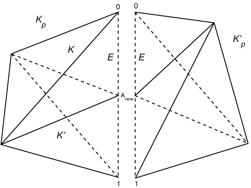
Fig. 6: The patch around a refinement edge EE with vertex 0 and 1. ℓ⁡(K)=ℓ⁡(K′)=L\ell(K)=\ell(K^{\prime})=L and ℓ⁡(Kp)=ℓ⁡(Kp′)=L−1\ell(K_{p})=\ell(K_{p}^{\prime})=L-1.
Proof.

We are going to prove the lemma by backward induction starting from l=Ll=L. Since ℳL=ℳh{\cal M}_{L}={\cal M}_{h} is conforming, for any K∈ℳLK\in{\cal M}_{L} satisfying ℓ⁡(K)=L\ell(K)=L, there exists a brother of KK, denoted by K′∈ℳLK^{\prime}\in{\cal M}_{L}, such that ℓ⁡(K′)=L\ell(K^{\prime})=L and Kp:=K∪K′∈ℳL−1K_{p}:=K\cup K^{\prime}\in{\cal M}_{L-1}. Here KpK_{p} is called the parent of KK and K′K^{\prime} with ℓ⁡(Kp)=L−1\ell(K_{p})=L-1 (see Fig. 6).

Let EE be the refinement edge of KpK_{p}. By the recursive bisection algorithm, EE must be the common refinement edge of all tetrahedra in the refinement patch:

PE=⋃{Kp′¯:Kp′∈ℳL−1​ and ​E⊂Kp′¯}.P_{E}=\bigcup\{\,\overline{K_{p}^{\prime}}:\;K_{p}^{\prime}\in{\cal M}_{L-1}\hbox{ and }E\subset\overline{K_{p}^{\prime}}\,\}.

By Lemma 8, ℓ⁡(Kp′)=L−1\ell(K_{p}^{\prime})=L-1 for any Kp′⊂PEK_{p}^{\prime}\subset P_{E} and the midpoint of EE, denoted by AnewA_{\mathrm{new}}, is the unique new vertex of ℳL{\cal M}_{L} in PEP_{E}. We conclude that

PE=⋃{K¯:K∈ℳL,ℓ(K)=L, and Anew is a vertex of K}.P_{E}=\bigcup\{\,\overline{K}:\;K\in{\cal M}_{L},\;\ell(K)=L,\hbox{ and }A_{\mathrm{new}}\hbox{ is a vertex of }K\,\}.

Coarsen the sub-mesh ℳL|PE{{\cal M}_{L}}_{|P_{E}} by removing the vertex AnewA_{\mathrm{new}} and all edges related to it and adding EE to this patch. Thus a conforming sub-mesh ℳL−1|PE{{\cal M}_{L-1}}_{|P_{E}} is obtained. Do the above coarsening process for every element K∈ℳLK\in{\cal M}_{L} with ℓ⁡(K)=L\ell(K)=L. This proves that ℳL−1{\cal M}_{L-1} is conforming.

Finally, an induction argument confirms that ℳl{\cal M}_{l} is conforming, l=L−2,⋯,1l=L-2,\cdots,1. ∎

4 Local multigrid

To begin with, we introduce nested refinement zones as open subsets of Ω\Omega:

(39) ωl:=interior(⋃{K¯:K∈ℳh,ℓ(K)≥l})⊂Ω,\displaystyle\omega_{l}:=\hbox{interior}\Big(\bigcup\{\overline{K}:\,K\in{\cal M}_{h},\,\ell(K)\geq l\}\Big)\subset{\Omega}\;,

see Fig. 7 and Fig. 8. The notion of refinement zones allows a concise definition of the local multilevel decompositions of the finite element spaces V⁡(ℳh)V({\cal M}_{h}) and 𝐔⁡(ℳh){\mathbf{U}}({\cal M}_{h}) that underly the local multigrid method.

Refer to caption

“Refinement strips”: set differences of refinement zones

Refer to caption : Σ0:=ω0∖ω1\Sigma_{0}:=\omega_{0}\setminus\omega_{1}
Refer to caption : Σ1:=ω1∖ω2\Sigma_{1}:=\omega_{1}\setminus\omega_{2}
Refer to caption : Σ2:=ω2∖ω3\Sigma_{2}:=\omega_{2}\setminus\omega_{3}
Refer to caption : Σ3:=ω3\Sigma_{3}:=\omega_{3}
Fig. 7: Refinement zones for the 2D refinement hierarchy of Figure 3.
Refer to caption

“Refinement strips”: set differences of refinement zones

Refer to caption : Σ0:=ω0∖ω1\Sigma_{0}:=\omega_{0}\setminus\omega_{1}
Refer to caption : Σ1:=ω1∖ω2\Sigma_{1}:=\omega_{1}\setminus\omega_{2}
Refer to caption : Σ2:=ω2∖ω3\Sigma_{2}:=\omega_{2}\setminus\omega_{3}
Refer to caption : Σ3:=ω3∖ω4\Sigma_{3}:=\omega_{3}\setminus\omega_{4}
Refer to caption : Σ4:=ω4∖ω5\Sigma_{4}:=\omega_{4}\setminus\omega_{5}
Refer to caption : Σ5:=ω5∖ω6\Sigma_{5}:=\omega_{5}\setminus\omega_{6}
Refer to caption : Σ6:=ω6\Sigma_{6}:=\omega_{6}
Fig. 8: Refinement zones for the 2D refinement hierarchy of Figure 5.

We introduce local multigrid from the perspective of multilevel successive subspace correction (SSC) [61, 62, 64]. First, we give an abstract description for a linear variational problem

(40) u∈H:𝖺⁡(u,v)=f⁡(v)∀v∈H,\displaystyle u\in H:\quad\mathsf{a}(u,v)=f(v)\quad\forall v\in H\;,

involving a positive definite bilinear form 𝖺\mathsf{a} on a Hilbert space HH. The method is completely defined after we have provided a finite subspace decomposition

(41) H=∑j=0JHj,Hj⊂Hclosed subspaces,j=0,…,J,J∈ℕ.\displaystyle H=\sum\limits_{j=0}^{J}H_{j}\;,\quad H_{j}\subset H\;\text{closed subspaces},\;j=0,\ldots,J,\;J\in\mathbb{N}\;.

Then the correction scheme implementation of one step of SSC acting on the iterate um−1u^{m-1} reads:

  • for m=1,2,⋯m=1,2,\cdots

    • u−1m−1=um−1u_{-1}^{m-1}=u^{m-1}

    • for j=0,1,⋯,Jj=0,1,\cdots,J

      • Let ej∈Hje_{j}\in H_{j} solve

        𝖺⁡(ej,vj)=f⁡(vj)−𝖺⁡(uj−1m−1,vj)∀vj∈Hj\mathsf{a}(e_{j},v_{j})=f(v_{j})-\mathsf{a}(u_{j-1}^{m-1},v_{j})\quad\forall\,v_{j}\in H_{j}
      • ujm−1=uj−1m−1+eju_{j}^{m-1}=u^{m-1}_{j-1}+e_{j}

    • endfor

    • um=uJm−1u^{m}=u^{m-1}_{J}

  • endfor

This amounts to a stationary linear iterative method with error propagation operator

(42) E=(I−PJ)(I−PJ−1)⋯(I−P0),\displaystyle E=(I-P_{J})(I-P_{J-1})\cdots(I-P_{0})\;,

where Pj:H↦HjP_{j}:H\mapsto H_{j} stands for the Galerkin projection defined through

(43) 𝖺⁡(Pj​v,vj)=𝖺⁡(v,vj)∀vj∈Hj.\mathsf{a}(P_{j}v,v_{j})=\mathsf{a}(v,v_{j})\quad\forall\,v_{j}\in H_{j}.

The convergence theory of SSC for an inner product 𝖺\mathsf{a} and induced energy norm ‖⋅‖A\left\|{\cdot}\right\|_{A} rests on two assumptions. The first one concerns the stability of the space decomposition. We assume that there exists a constant CstabC_{\mathrm{\scriptsize stab}} independent of JJ such that

(44) inf{∑j=0J‖vj‖A2:∑j=0Jvj=v}≤Cstab​‖v‖A2∀v∈H.\inf\Big\{\sum_{j=0}^{J}\left\|{v_{j}}\right\|_{A}^{2}:\;\sum_{j=0}^{J}v_{j}=v\Big\}\leq C_{\mathrm{\scriptsize stab}}\left\|{v}\right\|_{A}^{2}\quad\forall\,v\in H.

The second assumption is a strengthened Cauchy-Schwartz inequality, namely, there exist two constants 0≤q<10\leq q<1 and CorthC_{\mathrm{\scriptsize orth}} independent of jj and kk such that

(45) 𝖺⁡(vj,vk)≤Corth​q|k−j|​‖vj‖A​‖vk‖A∀vj∈Hj,vk∈Hk.\mathsf{a}(v_{j},v_{k})\leq C_{\mathrm{\scriptsize orth}}q^{|k-j|}\left\|{v_{j}}\right\|_{A}\left\|{v_{k}}\right\|_{A}\quad\forall\,v_{j}\in H_{j},\;v_{k}\in H_{k}\;.

The above inequality states a kind of quasi-orthogonality between the subspaces. From [61, Theorem 4.4] and [66, Theorem 5.1] we cite the following central convergence theorem:

Theorem 10.

Provided that (44) and (45) hold, the convergence rate of Algorithm SSC is bounded by

(46) ‖E‖A2≤1−1Cstab​(1+Θ)2withΘ=Corth​1+q1−q,\left\|{E}\right\|_{A}^{2}\leq 1-\frac{1}{C_{\mathrm{\scriptsize stab}}(1+\Theta)^{2}}\quad\hbox{with}\quad\Theta=C_{\mathrm{\scriptsize orth}}\frac{1+q}{1-q},

where the operator norm is defined by

‖E‖A:=supv∈H,v≠0‖E​v‖A‖v‖A.\left\|{E}\right\|_{A}:=\sup_{v\in H,v\neq 0}\frac{\left\|{Ev}\right\|_{A}}{\left\|{v}\right\|_{A}}.

The bottom line is that the subspace splitting (41) already provides a full description of the method. Showing that both constants CstabC_{\mathrm{\scriptsize stab}} from (44) and CorthC_{\mathrm{\scriptsize orth}} from (45) can be chosen independently of the number LL of refinement levels is the challenge in asymptotic multigrid analysis.

In concrete terms, the role of the linear variational problem (40) is played by (1) considered on the edge element space 𝐔⁡(ℳh){\mathbf{U}}({\cal M}_{h}), which replaces the Hilbert space HH. To define the local multilevel decomposition of 𝐔⁡(ℳh){\mathbf{U}}({\cal M}_{h}), we define “sets of new basis functions” on the various refinement levels

(47) 𝔅V0:=𝔅V(ℳ0),𝔅Vl:={bh∈𝔅V(ℳl):suppbh⊂ω¯l},𝔅𝐔0:=𝔅𝐔(ℳ0),𝔅𝐔l:={𝐛h∈𝔅𝐔(ℳl):supp𝐛h⊂ω¯l},1≤l≤L.\displaystyle\begin{aligned} &\mathfrak{B}_{V}^{0}:=\mathfrak{B}_{V}({\cal M}_{0}),\quad\mathfrak{B}_{V}^{l}:=\{b_{h}\in\mathfrak{B}_{V}({\cal M}_{l}):\;\mathop{\operator@font supp}\nolimits b_{h}\subset\overline{\omega}_{l}\}\;,\\ &\mathfrak{B}_{{\mathbf{U}}}^{0}:=\mathfrak{B}_{{\mathbf{U}}}({\cal M}_{0}),\quad\mathfrak{B}_{{\mathbf{U}}}^{l}:=\{{\mathbf{b}}_{h}\in\mathfrak{B}_{{\mathbf{U}}}({\cal M}_{l}):\;\mathop{\operator@font supp}\nolimits{\mathbf{b}}_{h}\subset\overline{\omega}_{l}\}\;,\end{aligned}\quad 1\leq l\leq L\;.

A 2D drawing of the sets 𝔅Vl\mathfrak{B}_{V}^{l} is given in Fig. 9 where ΓD=∂Ω\Gamma_{D}=\partial\Omega. Note that we also have to deal with V⁡(ℳh)V({\cal M}_{h}), because, as suggested by the reasoning in [29], a local multilevel decomposition of 𝐔⁡(ℳh){\mathbf{U}}({\cal M}_{h}) has to incorporate an appropriate local multilevel decomposition of V⁡(ℳh)V({\cal M}_{h}).

Refer to caption

l=0l=0

Refer to caption

l=1l=1

Refer to caption

l=2l=2

Refer to caption

l=3l=3

Fig. 9: Active vertices (red) carrying “tent functions” in 𝔅Vl\mathfrak{B}_{V}^{l}, ΓD=∂Ω\Gamma_{D}=\partial\Omega, refinement hierarchy of Fig. 3

Then, a possible local multigrid iteration for the linear system of equations arising from a finite element Galerkin discretization of a HΓD1​(Ω)H_{\Gamma_{D}}^{1}({\Omega})-elliptic variational problem boils down to a successive subspace correction method based on the local multilevel decomposition

(48) V⁡(ℳh)=V⁡(ℳ0)+∑l=1L∑bh∈𝔅VlSpan⁡{bh}.\displaystyle V({\cal M}_{h})=V({\cal M}_{0})+\sum\limits_{l=1}^{L}\sum\limits_{b_{h}\in\mathfrak{B}_{V}^{l}}\operatorname{Span}\left\{{b_{h}}\right\}\;.

Similarly, the local multilevel splitting of 𝐔⁡(ℳh){\mathbf{U}}({\cal M}_{h}) is based on the multilevel decomposition

(49) 𝐔⁡(ℳh)=𝐔⁡(ℳ0)+∑l=1L∑bh∈𝔅VlSpan⁡{𝐠𝐫𝐚𝐝⁡bh}+∑l=1L∑𝐛h∈𝔅𝐔lSpan⁡{𝐛h}.\displaystyle{\mathbf{U}}({\cal M}_{h})={\mathbf{U}}({\cal M}_{0})+\sum\limits_{l=1}^{L}\sum\limits_{b_{h}\in\mathfrak{B}_{V}^{l}}\operatorname{Span}\left\{{\operatorname{{\bf grad}}b_{h}}\right\}+\sum\limits_{l=1}^{L}\sum\limits_{{\mathbf{b}}_{h}\in\mathfrak{B}_{{\mathbf{U}}}^{l}}\operatorname{Span}\left\{{{\mathbf{b}}_{h}}\right\}\;.

These splittings induce SSC iterations that can be implemented as non-symmetric multigrid V-cycles with only one (hybrid) Gauss-Seidel post-smoothing step, see [29, Sect. 6]. Duplicating components of (49) results in more general multigrid cycles with various numbers of pre- and post-smoothing steps.

The splitting (49) is motivated both by the design of multigrid methods for (1) and 𝐔⁡(ℳ){\mathbf{U}}({\cal M}) in the case of uniform refinement and local multigrid approaches to HΓD1​(Ω)H_{\Gamma_{D}}^{1}({\Omega})-elliptic variational problems after discretization by means of linear finite elements [41, 60]. The occurrence of gradients of “tent functions” bhb_{h} in (49) is related to the hybrid local relaxation, which is essential for the performance of multigrid in 𝑯⁡(𝐜𝐮𝐫𝐥,Ω)\boldsymbol{H}(\operatorname{{\bf curl}},{\Omega}), see [29] for a rationale. A rigorous justification will emerge during the theoretical analysis in the following sections. It will establish the following main theorem.

Theorem 11 (Asymptotic convergence of local multigrid for edge elements).

Under the assumptions on the meshes made above and allowing at most one hanging node per edge, the decomposition (49) leads to an SSC iteration whose convergence rate is bounded away from 11 uniformly in the number LL of refinement steps.

5 Stability

First we tackle the stability estimate (44) for the local multilevel decomposition (48), which is implicitly contained in (49).

5.1 Local quasi-interpolation onto V⁡(ℳ)V({\cal M})

Quasi-interpolation operators are projectors onto finite element spaces that have been devised to accommodate two conflicting goals: locality and boundedness in weak norms [21, 46, 53, 50, 18]. As key tool they will be used in Sect. 5.2 and the proof of Lemma 21. As in [46, Sect. 2.1.1], we resort to a construction employing local linear L2L^{2}-dual basis functions. We follow the analysis of [50] that permits us to take into account Dirichlet boundary conditions.

For a generic tetrahedron KK define ψjK\psi^{K}_{j}, j=1,2,3,4j=1,2,3,4, by L2​(K)L^{2}(K)-duality to the barycentric coordinate functions λi\lambda_{i}, i=1,2,3,4i=1,2,3,4, of KK:

(50) ψjK∈ℙ1(K):∫KψjK(𝒙)λi(𝒙)d𝒙=δi​j,i,j∈{1,…,4}.\displaystyle\psi^{K}_{j}\in\mathbb{P}_{1}(K):\quad\int\nolimits_{K}\psi^{K}_{j}({\boldsymbol{x}})\lambda_{i}({\boldsymbol{x}})\,\mathrm{d}{\boldsymbol{x}}=\delta_{ij}\;,\quad i,j\in\{1,\ldots,4\}\;.

Computing an explicit representation of the ψjK\psi^{K}_{j} we find

(51) C−1≤|K|​‖ψjK‖L2​(K)2≤C,C−1≤‖ψjK‖L1​(K)≤C,\displaystyle C^{-1}\leq|K|\left\|{\psi^{K}_{j}}\right\|_{L^{2}({K})}^{2}\leq C\quad,\quad C^{-1}\leq\left\|{\psi^{K}_{j}}\right\|_{L^{1}({K})}\leq C\;,

with an absolute constant C>0C>0. We can regard ψjK\psi^{K}_{j} as belonging to the jj-th vertex of KK. Thus, we will also write ψ𝒑K\psi^{K}_{{\boldsymbol{p}}}, 𝒑∈𝒩⁡(K){\boldsymbol{p}}\in{\cal N}(K), 𝒩⁡(K){\cal N}(K) the set of vetices of KK.

Let ℳ{\cal M} be one of the tetrahedral meshes ℳl{\cal M}_{l} or ℳ^l\widehat{{\cal M}}_{l} of Ω\Omega. In order to introduce quasi-interpolation operators we take for granted some “node→\tocell”–assignment, a mapping 𝒩¯​(ℳ)↦ℳ\overline{{\cal N}}({\cal M})\mapsto{\cal M}, 𝒑∈𝒩¯​(ℳ)↦K𝒑∈ℳ{\boldsymbol{p}}\in\overline{{\cal N}}({\cal M})\mapsto K_{{\boldsymbol{p}}}\in{\cal M}.

Definition 12.

Writing {b𝐩}𝐩∈𝒩⁡(ℳ):=𝔅V​(ℳ){\{b_{{\boldsymbol{p}}}\}}_{{\boldsymbol{p}}\in{\cal N}({{\cal M}})}:=\mathfrak{B}_{V}({{\cal M}}), define the local quasi-interpolation operator

(52) 𝖰h:{L2​(Ω)↦V⁡(ℳ)u↦∑𝒑∈𝒩⁡(ℳ)∫K𝒑ψ𝒑K𝒑​(𝒙)​u​(𝒙)​d𝒙⋅b𝒑.\mathsf{Q}_{h}:\left\{\begin{array}[]{ccl}\displaystyle L^{2}({\Omega})&\mapsto&V({{\cal M}})\\ \displaystyle u&\mapsto&\sum_{{\boldsymbol{p}}\in\mathcal{N}({{\cal M}})}\int_{K_{{\boldsymbol{p}}}}\psi^{K_{{{\boldsymbol{p}}}}}_{{\boldsymbol{p}}}({\boldsymbol{x}})u({\boldsymbol{x}})\,d{\boldsymbol{x}}\cdot b_{{{\boldsymbol{p}}}}\;.\end{array}\right.

Analoguously, we introduce the local quasi-interpolation 𝖰¯h:L2​(Ω)↦V¯​(ℳ)\overline{\mathsf{Q}}_{h}:L^{2}({\Omega})\mapsto\overline{V}({\cal M}).

We point out that 𝖰h\mathsf{Q}_{h} respects u=0u=0 on ΓD\Gamma_{D}, because the sum does not cover basis functions attached to vertices on ΓD\Gamma_{D}. From (50) it is also evident that both 𝖰h\mathsf{Q}_{h} and 𝖰¯h\overline{\mathsf{Q}}_{h} are projections, for instance,

(53) 𝖰h​uh=uh∀uh∈V⁡(ℳ).\mathsf{Q}_{h}u_{h}=u_{h}\quad\forall\,u_{h}\in V({{\cal M}})\;.

Moreover, they satisfy the following strong continuity and approximation properties:

Lemma 13.

The quasi-interpolation operators from Def. 12 allow the estimates (set ΓD=∅\Gamma_{D}=\emptyset for 𝖰¯ℳ\overline{\mathsf{Q}}_{{\cal M}})

(54) ∃C=C⁡(ρℳ):‖𝖰h​u‖L2​(Ω)≤C​‖u‖L2​(Ω)​∀u∈L2​(Ω),\displaystyle\exists C=C(\rho_{{{\cal M}}}):\qquad\qquad\;\;\;\left\|{\mathsf{Q}_{h}u}\right\|_{L^{2}({\Omega})}\leq C\left\|{u}\right\|_{L^{2}({\Omega})}\;\;\,\forall\,u\in L^{2}({\Omega})\;,
(55) ∃C=C⁡(ρℳ,Ω,ΓD):|𝖰h​u|H1​(Ω)≤C​|u|H1​(Ω)∀u∈HΓD1​(Ω),\displaystyle\exists C=C(\rho_{{{\cal M}}},\Omega,\Gamma_{D}):\quad\quad\;{\left|{\mathsf{Q}_{h}u}\right|}_{H^{1}({\Omega})}\leq C{\left|{u}\right|}_{H^{1}({\Omega})}\quad\;\forall\,u\in H_{\Gamma_{D}}^{1}({\Omega})\;,
(56) ∃C=C⁡(ρℳ,k):‖h−k​(u−𝖰h​u)‖L2​(Ω)≤C​|u|Hk​(Ω)∀u∈Hk​(Ω)∩HΓD1​(Ω),\displaystyle\exists C=C(\rho_{{{\cal M}}},k):\;\left\|{h^{-k}(u-\mathsf{Q}_{h}u)}\right\|_{L^{2}({\Omega})}\leq C{\left|{u}\right|}_{H^{k}({\Omega})}\quad\forall\,u\in H^{k}({\Omega})\cap H_{\Gamma_{D}}^{1}({\Omega})\;,

and k=1,2k=1,2.

Part I.

Continuity in L2​(Ω)L^{2}({\Omega}) is a simple consequence of the stability (16) of the nodal bases 𝔅V​(ℳ)\mathfrak{B}_{V}({{\cal M}}) and of the Cauchy-Schwarz inequality:

‖𝖰h​u‖L2​(Ω)2\displaystyle\left\|{\mathsf{Q}_{h}u}\right\|_{L^{2}({\Omega})}^{2} ≤\displaystyle\leq C​∑𝒑∈𝒩⁡(ℳ)|𝖰h​u​(𝒑)|2​‖b𝒑‖L2​(Ω)2\displaystyle C\sum\limits_{{\boldsymbol{p}}\in{\cal N}({{\cal M}})}|\mathsf{Q}_{h}u({\boldsymbol{p}})|^{2}\left\|{b_{{\boldsymbol{p}}}}\right\|_{L^{2}({\Omega})}^{2}
=\displaystyle= C​∑𝒑∈𝒩⁡(ℳ)|∫K𝒑ψ𝒑K𝒑​(𝒙)​u​(𝒙)​𝑑𝒙|2​‖b𝒑‖L2​(Ω)2\displaystyle C\hskip-4.30554pt\sum\limits_{{\boldsymbol{p}}\in{\cal N}({{\cal M}})}\left|\int\nolimits_{K_{{\boldsymbol{p}}}}\psi^{K_{{{\boldsymbol{p}}}}}_{{\boldsymbol{p}}}({\boldsymbol{x}})u({\boldsymbol{x}})\,d{\boldsymbol{x}}\right|^{2}\left\|{b_{{\boldsymbol{p}}}}\right\|_{L^{2}({\Omega})}^{2}
≤\displaystyle\leq C​∑𝒑∈𝒩⁡(ℳ)‖ψ𝒑K𝒑‖L2​(K𝒑)2​‖b𝒑‖L2​(Ω)2​‖u‖L2​(K𝒑)2≤C​‖u‖L2​(Ω)2,\displaystyle C\sum\limits_{{\boldsymbol{p}}\in{\cal N}({{\cal M}})}\left\|{\psi^{K_{{\boldsymbol{p}}}}_{{\boldsymbol{p}}}}\right\|_{L^{2}({K_{{\boldsymbol{p}}}})}^{2}\left\|{b_{{\boldsymbol{p}}}}\right\|_{L^{2}({\Omega})}^{2}\left\|{u}\right\|_{L^{2}({K_{{\boldsymbol{p}}}})}^{2}\leq C\left\|{u}\right\|_{L^{2}({\Omega})}^{2}\;,

with C=C⁡(ρℳ)>0C=C(\rho_{{{\cal M}}})>0, because ‖ψ𝒑K𝒑‖L2​(K𝒑)2​‖b𝒑‖L2​(Ω)2≤C\left\|{\psi^{K_{{\boldsymbol{p}}}}_{{\boldsymbol{p}}}}\right\|_{L^{2}({K_{{\boldsymbol{p}}}})}^{2}\left\|{b_{{\boldsymbol{p}}}}\right\|_{L^{2}({\Omega})}^{2}\leq C, too. ∎

The following estimate is instrumental in establishing continuity of 𝖰h\mathsf{Q}_{h} in HΓD1​(Ω)H_{\Gamma_{D}}^{1}({\Omega}):

Theorem 14 (Generalized Hardy inquality).
∃C=C⁡(Ω,ΓD)>0:∫Ω|udist⁡(𝒙,ΓD)|2​𝑑𝒙≤C​|u|H1​(Ω)2∀u∈HΓD1​(Ω).\displaystyle\exists C=C(\Omega,\Gamma_{D})>0:\quad\int\limits_{\Omega}\left|\frac{u}{\operatorname{dist}({\boldsymbol{x}},\Gamma_{D})}\right|^{2}\,\mathrm{d}{\boldsymbol{x}}\leq C{\left|{u}\right|}_{H^{1}({\Omega})}^{2}\quad\forall u\in H_{\Gamma_{D}}^{1}({\Omega})\;.
Proof.

By density it suffices to consider u∈C∞​(Ω¯)u\in C^{\infty}(\overline{\Omega}), supp⁡(u)∩ΓD=∅\operatorname{supp}(u)\cap\Gamma_{D}=\emptyset. Using a partition of unity, we can confine the estimate to neighborhoods of ΓD\Gamma_{D}, in which ∂Ω\partial\Omega is the graph of a Lipschitz-continuous function. Thus, after bi-Lipschitz transformations, we need only investigate three canonical situations, see Fig. 10:

  1. 1.

    ΓD={z=0}\Gamma_{D}=\{z=0\}, for which the 1D Hardy inequality gives the estimate, see the proof of Thm. 1.4.4.4 in [27].

  2. 2.

    ΓD={z=0∧x>0}\Gamma_{D}=\{z=0\;\wedge\;x>0\}, which can be treated using polar coordinates in the (x,z)(x,z)-plane and then integrating in yy-direction:

    ​∫0∞∫0π|u⁡(r,φ)r|2​𝑑φ​r​𝑑r≤∫0∞∫0π|πr​∂u∂φ​(r,φ)|2​𝑑φ​r​𝑑r≤π2​∫z>0|𝐠𝐫𝐚𝐝x,z⁡u|2​𝑑x​𝑑z.\displaystyle\mbox{$$}\hskip-20.00003pt\int\limits_{0}^{\infty}\int\limits_{0}^{\pi}\left|\frac{u(r,\varphi)}{r}\right|^{2}\mathrm{d}\varphi\,r\,\mathrm{d}r\leq\int\limits_{0}^{\infty}\int\limits_{0}^{\pi}\left|\frac{\pi}{r}\frac{\partial u}{\partial\varphi}(r,\varphi)\right|^{2}\mathrm{d}\varphi\,r\,\mathrm{d}r\leq\pi^{2}\int\limits_{z>0}|\operatorname{{\bf grad}}_{x,z}u|^{2}\,\mathrm{d}x\mathrm{d}z\;.
  3. 3.

    ΓD={z=0∧x>0∧y>0}\Gamma_{D}=\{z=0\,\wedge x>0\,\wedge\,y>0\}, for which we obtain a similar estimate using spherical coordinates.

This ends the proof. ∎

Refer to caption

ΓD={z=0}\Gamma_{D}=\{z=0\}

Refer to caption

ΓD={z=0∧x>0}\Gamma_{D}=\{z=0\,\wedge\,x>0\}

Refer to caption

ΓD={z=0∧x>0∧y>0}\Gamma_{D}=\{z=0\,\wedge x>0\,\wedge\,y>0\}

Fig. 10: Canonical situations to be examined in the proof of Thm. 14
of Lemma 13, part II.

In order to tackle the H1​(Ω)H^{1}({\Omega})-continuity of 𝖰h\mathsf{Q}_{h}, we use that 𝐠𝐫𝐚𝐝⁡V⁡(ℳ)⊂𝐔⁡(ℳ)\operatorname{{\bf grad}}V({\cal M})\subset{\mathbf{U}}({\cal M}) along with the stability estimate (12)

(57) ‖𝐠𝐫𝐚𝐝⁡𝖰h​u‖L2​(Ω)2≤C​∑E=[𝒑,𝒒]∈ℰ⁡(ℳ)(𝖰h​u​(𝒑)−𝖰h​u​(𝒒))2​‖𝐛E‖L2​(Ω)2,\displaystyle\left\|{\operatorname{{\bf grad}}\mathsf{Q}_{h}u}\right\|_{L^{2}({\Omega})}^{2}\leq C\sum\limits_{E=[{\boldsymbol{p}},{\boldsymbol{q}}]\in{\cal E}({{\cal M}})}(\mathsf{Q}_{h}u({\boldsymbol{p}})-\mathsf{Q}_{h}u({\boldsymbol{q}}))^{2}\left\|{{\mathbf{b}}_{E}}\right\|_{L^{2}({\Omega})}^{2}\;,

with the notation {𝐛E}E∈ℰ⁡(ℳ):=𝔅𝐔​(ℳ){\{{\mathbf{b}}_{E}\}}_{E\in{\cal E}({{\cal M}})}:=\mathfrak{B}_{{\mathbf{U}}}({{\cal M}}).

(i) for the case E=[𝒑,𝒒]∈ℰ⁡(ℳ)E=[{\boldsymbol{p}},{\boldsymbol{q}}]\in{\cal E}({{\cal M}}), 𝒑,𝒒∉ΓD{\boldsymbol{p}},{\boldsymbol{q}}\not\in\Gamma_{D}, we adapt arguments from [50]. For any u∈HΓD1​(Ω)u\in H_{\Gamma_{D}}^{1}({\Omega}), by (50), we have the identity

|(𝖰h​u)​(𝒑)−(𝖰h​u)​(𝒒)|=|∫K𝒑∫K𝒒ψ𝒑K𝒑​(𝒙)​ψ𝒒K𝒒​(𝒚)​(u⁡(𝒙)−u⁡(𝒚))​𝑑𝒚​𝑑𝒙|=|∫K𝒑∫K𝒒ψ𝒑K𝒑​(𝒙)​ψ𝒒K𝒒​(𝒚)​∫01𝐠𝐫𝐚𝐝⁡u⁡(𝒚+τ⁡(𝒙−𝒚))⋅(𝒙−𝒚)​dτ​d𝒚​d𝒙|.|(\mathsf{Q}_{h}u)({\boldsymbol{p}})-(\mathsf{Q}_{h}u)({\boldsymbol{q}})|=\Bigl|\int\limits_{K_{{\boldsymbol{p}}}}\int\limits_{K_{{\boldsymbol{q}}}}\psi_{{\boldsymbol{p}}}^{K_{{\boldsymbol{p}}}}({\boldsymbol{x}})\psi_{{\boldsymbol{q}}}^{K_{{\boldsymbol{q}}}}({\boldsymbol{y}})(u({\boldsymbol{x}})-u({\boldsymbol{y}}))\,\mathrm{d}{\boldsymbol{y}}\mathrm{d}{\boldsymbol{x}}\Bigr|\\ =\Bigl|\int\limits_{K_{{\boldsymbol{p}}}}\int\limits_{K_{{\boldsymbol{q}}}}\psi_{{\boldsymbol{p}}}^{K_{{\boldsymbol{p}}}}({\boldsymbol{x}})\psi_{{\boldsymbol{q}}}^{K_{{\boldsymbol{q}}}}({\boldsymbol{y}})\,\int\limits_{0}^{1}\operatorname{{\bf grad}}u({\boldsymbol{y}}+\tau({\boldsymbol{x}}-{\boldsymbol{y}}))\cdot({\boldsymbol{x}}-{\boldsymbol{y}})\,\mathrm{d}\tau\,\mathrm{d}{\boldsymbol{y}}\mathrm{d}{\boldsymbol{x}}\Bigr|\;.

Then split the innermost integral and transform

∫01f⁡(𝒚+τ⁡(𝒙−𝒚))​𝑑τ=∫121f⁡(𝒚+τ⁡(𝒙−𝒚))​𝑑τ+∫121f⁡(𝒙+τ⁡(𝒚−𝒙))​𝑑τ.\displaystyle\int\nolimits_{0}^{1}f({\boldsymbol{y}}+\tau({\boldsymbol{x}}-{\boldsymbol{y}}))\,\mathrm{d}\tau=\int\nolimits_{\frac{1}{2}}^{1}f({\boldsymbol{y}}+\tau({\boldsymbol{x}}-{\boldsymbol{y}}))\,\mathrm{d}\tau+\int\nolimits_{\frac{1}{2}}^{1}f({\boldsymbol{x}}+\tau({\boldsymbol{y}}-{\boldsymbol{x}}))\,\mathrm{d}\tau\;.

We infer

|(𝖰h​u)​(𝒑)−(𝖰h​u)​(𝒒)|≤∫121∫K𝒑∫K𝒒|ψ𝒑K𝒑​(𝒙)|​|ψ𝒒K𝒒​(𝒚)|​|𝐠𝐫𝐚𝐝⁡u⁡(𝒚+τ⁡(𝒙−𝒚))|​|𝒙−𝒚|​𝑑𝒚​𝑑𝒙​𝑑τ+∫121∫K𝒑∫K𝒒|ψ𝒑K𝒑​(𝒙)|​|ψ𝒒K𝒒​(𝒚)|​|𝐠𝐫𝐚𝐝⁡u⁡(𝒙+τ⁡(𝒚−𝒙))|​|𝒙−𝒚|​𝑑𝒚​𝑑𝒙​𝑑τ|(\mathsf{Q}_{h}u)({\boldsymbol{p}})-(\mathsf{Q}_{h}u)({\boldsymbol{q}})|\\ \leq\begin{aligned} &\int\limits_{\frac{1}{2}}^{1}\int\limits_{K_{{\boldsymbol{p}}}}\int\limits_{K_{{\boldsymbol{q}}}}|\psi_{{\boldsymbol{p}}}^{K_{{\boldsymbol{p}}}}({\boldsymbol{x}})||\psi_{{\boldsymbol{q}}}^{K_{{\boldsymbol{q}}}}({\boldsymbol{y}})|\,|\operatorname{{\bf grad}}u({\boldsymbol{y}}+\tau({\boldsymbol{x}}-{\boldsymbol{y}}))||{\boldsymbol{x}}-{\boldsymbol{y}}|\,\mathrm{d}{\boldsymbol{y}}\mathrm{d}{\boldsymbol{x}}\mathrm{d}\tau\\ +&\int\limits_{\frac{1}{2}}^{1}\int\limits_{K_{{\boldsymbol{p}}}}\int\limits_{K_{{\boldsymbol{q}}}}|\psi_{{\boldsymbol{p}}}^{K_{{\boldsymbol{p}}}}({\boldsymbol{x}})||\psi_{{\boldsymbol{q}}}^{K_{{\boldsymbol{q}}}}({\boldsymbol{y}})|\,|\operatorname{{\bf grad}}u({\boldsymbol{x}}+\tau({\boldsymbol{y}}-{\boldsymbol{x}}))|\,|{\boldsymbol{x}}-{\boldsymbol{y}}|\,\mathrm{d}{\boldsymbol{y}}\mathrm{d}{\boldsymbol{x}}\mathrm{d}\tau\end{aligned}

The transformation formula for integrals reveals

∫Kf⁡(𝒙+τ⁡(𝒚−𝒙))​𝑑𝒚=τ−3​∫K′f⁡(𝒛)​𝑑𝒛,K′:=𝒙+τ⁡(K−𝒙).\displaystyle\int\nolimits_{K}f({\boldsymbol{x}}+\tau({\boldsymbol{y}}-{\boldsymbol{x}}))\,\mathrm{d}{\boldsymbol{y}}=\tau^{-3}\int\nolimits_{K^{\prime}}f({\boldsymbol{z}})\,\mathrm{d}{\boldsymbol{z}}\;,\quad K^{\prime}:={\boldsymbol{x}}+\tau(K-{\boldsymbol{x}})\;.

Appealing to the bounds for ‖ψjK‖L2​(K)\left\|{\psi_{j}^{K}}\right\|_{L^{2}({K})}, ‖ψjK‖L1​(K)\left\|{\psi_{j}^{K}}\right\|_{L^{1}({K})}, K∈ℳK\in{{\cal M}}, from (51), the Cauchy-Schwarz inequality yields

(58) |(𝖰h​u)​(𝒑)−(𝖰h​u)​(𝒒)|​‖𝐛E‖L2​(Ω)\displaystyle|(\mathsf{Q}_{h}u)({\boldsymbol{p}})-(\mathsf{Q}_{h}u)({\boldsymbol{q}})|\left\|{{\mathbf{b}}_{E}}\right\|_{L^{2}({\Omega})}
≤C[|𝒑−𝒒|​‖𝐛E‖L2​(Ω)min⁡{|K𝒒|12,|K𝒑|12}]⏟≤C=C⁡(ρℳ)∫121τ−3/2dτ⋅|u|H1​(⟨ΩE⟩).\displaystyle\qquad\qquad\leq C\underbrace{\left[\frac{|{\boldsymbol{p}}-{\boldsymbol{q}}|\left\|{{\mathbf{b}}_{E}}\right\|_{L^{2}({\Omega})}}{\min\{|K_{{\boldsymbol{q}}}|^{\frac{1}{2}},|K_{{\boldsymbol{p}}}|^{\frac{1}{2}}\}}\right]}_{{\leq C=C(\rho_{{{\cal M}}})}}\int\nolimits_{\frac{1}{2}}^{1}\tau^{-3/2}\,\mathrm{d}\tau\cdot{\left|{u}\right|}_{H^{1}({\left<\Omega_{E}\right>})}\;.

Here ⟨ΩE⟩\left<\Omega_{E}\right> stands for the convex hull of all tetrahedra adjacent to the edge EE.

(ii) now consider E=[𝒑,𝒒]∈ℰ⁡(ℳ)E=[{\boldsymbol{p}},{\boldsymbol{q}}]\in{\cal E}({\cal M}), 𝒑∈ΓD{\boldsymbol{p}}\in\Gamma_{D}. Then, for any u∈HΓD1​(Ω)u\in H_{\Gamma_{D}}^{1}({\Omega})

|(𝖰h​u)​(𝒒)−(𝖰h​u)​(𝒑)|2=|(𝖰h​u)​(𝒒)|2=|∫K𝒒ψ𝒒K𝒒​(𝒙)​u​(𝒙)​𝑑𝒙|2\displaystyle|(\mathsf{Q}_{h}u)({\boldsymbol{q}})-(\mathsf{Q}_{h}u)({\boldsymbol{p}})|^{2}=|(\mathsf{Q}_{h}u)({\boldsymbol{q}})|^{2}=\left|\int\nolimits_{K_{{\boldsymbol{q}}}}\psi_{{\boldsymbol{q}}}^{K_{{\boldsymbol{q}}}}({\boldsymbol{x}})u({\boldsymbol{x}})\,\mathrm{d}{\boldsymbol{x}}\right|^{2}
=\displaystyle= |∫K𝒒dist⁡(𝒙,ΓD)⏟≤C​|𝒑−𝒒|​ψ𝒒K𝒒​(𝒙)​u⁡(𝒙)dist⁡(𝒙,ΓD)​𝑑𝒙|2≤C​|𝒑−𝒒|2|K𝒒|⋅∫K𝒒|u⁡(𝒙)dist⁡(𝒙,ΓD)|2​𝑑𝒙\displaystyle\Bigl|\int\nolimits_{K_{{\boldsymbol{q}}}}\underbrace{\operatorname{dist}({\boldsymbol{x}},\Gamma_{D})}_{\leq C|{\boldsymbol{p}}-{\boldsymbol{q}}|}\psi_{{\boldsymbol{q}}}^{K_{{\boldsymbol{q}}}}({\boldsymbol{x}})\frac{u({\boldsymbol{x}})}{\operatorname{dist}({\boldsymbol{x}},\Gamma_{D})}\,\mathrm{d}{\boldsymbol{x}}\Bigr|^{2}\leq\frac{C|{\boldsymbol{p}}-{\boldsymbol{q}}|^{2}}{|K_{{\boldsymbol{q}}}|}\cdot\int\limits_{K_{{\boldsymbol{q}}}}\left|\frac{u({\boldsymbol{x}})}{\operatorname{dist}({\boldsymbol{x}},\Gamma_{D})}\right|^{2}\,\mathrm{d}{\boldsymbol{x}}
≤\displaystyle\leq C|𝒑−𝒒|​∫ΩE|u⁡(𝒙)dist⁡(𝒙,ΓD)|2​𝑑𝒙,\displaystyle\frac{C}{|{\boldsymbol{p}}-{\boldsymbol{q}}|}\int\limits_{\Omega_{E}}\left|\frac{u({\boldsymbol{x}})}{\operatorname{dist}({\boldsymbol{x}},\Gamma_{D})}\right|^{2}\,\mathrm{d}{\boldsymbol{x}}\;,

with (different) constants C=C⁡(ρℳ)>0C=C(\rho_{{{\cal M}}})>0.

Combining (57), (58), using the finite overlap property of ℳ{{\cal M}} in the form

∃C=C⁡(ρℳ):♯⁡{E∈ℰ⁡(ℳ):𝒙∈⟨ΩE⟩}≤C∀𝒙∈Ω,\displaystyle\exists C=C(\rho_{{{\cal M}}}):\quad\sharp\{E\in{\cal E}({{\cal M}}):\,{\boldsymbol{x}}\in\left<\Omega_{E}\right>\}\leq C\quad\forall{\boldsymbol{x}}\in\Omega\;,

and appealing to Thm. 14 confirm |𝖰h​u|H1​(Ω)≤C​|u|H1​(Ω){\left|{\mathsf{Q}_{h}u}\right|}_{H^{1}({\Omega})}\leq C{\left|{u}\right|}_{H^{1}({\Omega})}. Observe that the Hardy inequality makes the constant depend on Ω\Omega and ΓD\Gamma_{D} in addition.

The quasi-interpolation error estimate (56) results from scaling arguments. Pick K∈ℳK\in{\cal M}, u∈H2​(Ω)∩HΓD1​(Ω)u\in H^{2}({\Omega})\cap H_{\Gamma_{D}}^{1}({\Omega}), and write ℐK​u∈ℙ1​(K){\cal I}_{K}u\in\mathbb{P}_{1}(K) for the linear interpolant of uu on KK. Thanks to the projection property, we deduce as in Part I of the proof that, with C=C⁡(ρℳ)C=C(\rho_{{\cal M}}),

‖(I​d−𝖰h)​u‖L2​(K)\displaystyle\left\|{(Id-\mathsf{Q}_{h})u}\right\|_{L^{2}({K})} =\displaystyle= ‖(I​d−𝖰h)​(u−ℐK​u)‖L2​(K)≤C​‖u−ℐK​u‖L2​(ΩK)\displaystyle\left\|{(Id-\mathsf{Q}_{h})(u-{\cal I}_{K}u)}\right\|_{L^{2}({K})}\leq C\left\|{u-{\cal I}_{K}u}\right\|_{L^{2}({\Omega_{K}})}
≤\displaystyle\leq C​hK2​|u|H2​(ΩK).\displaystyle Ch_{K}^{2}{\left|{u}\right|}_{H^{2}({\Omega_{K}})}\;.

Here, we wrote ΩK:=⋃{K′¯:K′¯∩K≠∅}\Omega_{K}:=\bigcup\{\overline{K^{\prime}}:\,\overline{K^{\prime}}\cap K\not=\emptyset\}, and the final estimate can be shown by a simple scaling argument, cf. (17). Estimate (56) for k=1k=1 follows by scaling arguments and interpolation between the Sobolev spaces H2​(ΩK)H^{2}(\Omega_{K}) and L2​(ΩK)L^{2}(\Omega_{K}). ∎

5.2 Multilevel splitting of V⁡(ℳL)V({{{\cal M}}_{L}})

In this section we first revisit the well-known [61, 45, 67] uniform stability of multilevel splittings of H1​(Ω)H^{1}({\Omega})-conforming Lagrangian finite element functions in the case of mesh hierarchies generated by uniform, i.e. non-local, regular refinement.

We take for granted a virtual refinement hierarchy (34) of tetrahedral meshes as introduced in Sect. 3 and its accompanying quasi-uniform family of meshes (35).

Owing to the inf\inf in (44), it is enough to find a concrete family of admissible “candidate” decompositions that enjoys the desired LL-uniform stability. We aim for candidates that fit the locally refined mesh hierarchy.

The principal idea, borrowed from [46, Sect. 4.2.2], is to use a sequence of quasi-interpolation operators 𝖰l:L2​(Ω)↦V⁡(ℳ^l)\mathsf{Q}_{l}:L^{2}({\Omega})\mapsto V(\widehat{{\cal M}}_{l}) based on a judiciously chosen node→\toelement–assignments. For ℳ^l\widehat{{\cal M}}_{l} we introduce a “coarsest neighbor node→\toelement–assignment”: First, for any 𝒑∈𝒩⁡(ℳ^l){\boldsymbol{p}}\in{\cal N}(\widehat{{\cal M}}_{l}), l=1,…,Ll=1,\ldots,L, we pick K∈ℳlK\in{{\cal M}}_{l} such that

ℓ(K)=min{ℓ(K):𝒑∈K¯,K∈ℳl}.\displaystyle\ell(K)=\min\{\ell(K):\;{\boldsymbol{p}}\in\overline{K},\;K\in{\cal M}_{l}\}\;.

Secondly, we select a “coarsest neighbor” K𝒑∈ℳ^lK_{{\boldsymbol{p}}}\in\widehat{{\cal M}}_{l} among those elements of ℳ^l\widehat{{\cal M}}_{l} that are contained in KK. This defines a mapping 𝒩⁡(ℳ^l)↦ℳl^{\cal N}(\widehat{{\cal M}}_{l})\mapsto\widehat{{\cal M}_{l}}, 𝒑↦K𝒑{\boldsymbol{p}}\mapsto K_{{\boldsymbol{p}}}. We write 𝖰¯l:L2​(Ω)↦V¯​(ℳ^l)\overline{\mathsf{Q}}_{l}:L^{2}({\Omega})\mapsto\overline{V}(\widehat{{\cal M}}_{l}) for the induced quasi-interpolation operator according to Def. 12.

Next, we examine the candidate multilevel splitting

(59) uh=𝖰¯0​uh+∑l=1L(𝖰¯l−𝖰¯l−1)​uh,uh∈V⁡(ℳ^L).\displaystyle u_{h}=\overline{\mathsf{Q}}_{0}u_{h}+\sum\limits_{l=1}^{L}(\overline{\mathsf{Q}}_{l}-\overline{\mathsf{Q}}_{l-1})u_{h}\;,\quad u_{h}\in V(\widehat{{\cal M}}_{L})\;.
Lemma 15.

There holds, with a constant C>0C>0 depending only on Ω\Omega and the uniform bound for the shape regularity measures ρℳ^l\rho_{\widehat{{\cal M}}_{l}}, 0≤l≤L0\leq l\leq L,

(60) |𝖰¯0​uh|H1​(Ω)2+∑l=1Lhl−2​‖(𝖰¯l−𝖰¯l−1)​uh‖L2​(Ω)2≤C​|uh|H1​(Ω)2∀uh∈V⁡(ℳ^L).{\left|{\overline{\mathsf{Q}}_{0}u_{h}}\right|}_{H^{1}({\Omega})}^{2}+\sum_{l=1}^{L}h_{l}^{-2}\left\|{(\overline{\mathsf{Q}}_{l}-\overline{\mathsf{Q}}_{l-1})u_{h}}\right\|_{L^{2}({\Omega})}^{2}\leq C{\left|{u_{h}}\right|}_{H^{1}({\Omega})}^{2}\quad\forall u_{h}\in V(\widehat{{\cal M}}_{L})\;.
Proof.

We take the cue from the elegant approach of Bornemann and Yserentant in [11], who discovered how to bring techniques of real interpolation theory of Sobolev spaces [37], [39, Appendix B] to bear on (59). The main tools are the so-called KK-functionals given by

K​(t,u)2\displaystyle K(t,u)^{2} :⁣=\displaystyle:= infw∈H2​(Ω){‖u−w‖L2​(Ω)2+t2​|w|H2​(Ω)2},\displaystyle\inf_{w\in H^{2}(\Omega)}\left\{\left\|{u-w}\right\|_{L^{2}({\Omega})}^{2}+t^{2}\left|{w}\right|^{2}_{H^{2}(\Omega)}\right\}\;,
Kℝ3​(t,u)2\displaystyle K_{\mathbb{R}^{3}}(t,u)^{2} :⁣=\displaystyle:= infw∈H2​(ℝ3){‖u−w‖L2​(ℝ3)2+t2​|w|H2​(ℝ3)2}.\displaystyle\inf_{w\in H^{2}(\mathbb{R}^{3})}\left\{\left\|{u-w}\right\|^{2}_{L^{2}(\mathbb{R}^{3})}+t^{2}\left|{w}\right|^{2}_{H^{2}(\mathbb{R}^{3})}\right\}\;.

The estimates (55) and (56) of Lemma 13 create a link between the terms in (60) and K⁡(t,u)K(t,u): owing to (54) and (56) there holds for any u∈L2​(Ω)u\in L^{2}({\Omega})

‖(𝖰¯l−𝖰¯l−1)​u‖L2​(Ω)\displaystyle\left\|{(\overline{\mathsf{Q}}_{l}-\overline{\mathsf{Q}}_{l-1})u}\right\|_{L^{2}({\Omega})} ≤\displaystyle\leq ‖(𝖰¯l−𝖰¯l−1)​(u−w)‖L2​(Ω)+‖(𝖰¯l−𝖰¯l−1)​w‖L2​(Ω)\displaystyle\left\|{(\overline{\mathsf{Q}}_{l}-\overline{\mathsf{Q}}_{l-1})(u-w)}\right\|_{L^{2}({\Omega})}+\left\|{(\overline{\mathsf{Q}}_{l}-\overline{\mathsf{Q}}_{l-1})w}\right\|_{L^{2}({\Omega})}
≤\displaystyle\leq C⁡(‖u−w‖L2​(Ω)+hl2​|w|H2​(Ω))∀w∈H2​(Ω).\displaystyle C\bigl(\left\|{u-w}\right\|_{L^{2}({\Omega})}+h_{l}^{2}{\left|{w}\right|}_{H^{2}({\Omega})}\bigr)\quad\forall w\in H^{2}({\Omega})\;.

Here and below the generic constants CC may depend on shape regularity max0≤l≤L⁡ρℳ^l\max\limits_{0\leq l\leq L}\rho_{\widehat{{\cal M}}_{l}} and the (quasi-uniformity) constants in (36). We conclude

(61) ‖(𝖰¯l−𝖰¯l−1)​u‖L2​(Ω)2≤C​K​(hl2,u)2∀u∈L2​(Ω),\displaystyle\left\|{(\overline{\mathsf{Q}}_{l}-\overline{\mathsf{Q}}_{l-1})u}\right\|_{L^{2}({\Omega})}^{2}\leq C\,K(h_{l}^{2},u)^{2}\quad\forall u\in L^{2}({\Omega})\;,

which implies

(62) |𝖰¯0​u|H1​(Ω)2+∑l=1Lhl−2​‖(𝖰¯l−𝖰¯l−1)​u‖L2​(Ω)2≤C⁡{|u|H1​(Ω)2+∑l=1Lhl−2​K​(hl2,u)}.{\left|{\overline{\mathsf{Q}}_{0}u}\right|}_{H^{1}({\Omega})}^{2}+\sum_{l=1}^{L}h_{l}^{-2}\left\|{(\overline{\mathsf{Q}}_{l}-\overline{\mathsf{Q}}_{l-1})u}\right\|_{L^{2}({\Omega})}^{2}\leq C\Big\{{\left|{u}\right|}_{H^{1}({\Omega})}^{2}+\sum_{l=1}^{L}h_{l}^{-2}K(h^{2}_{l},u)\Big\}\;.

Let u~∈H1​(ℝ3)\widetilde{u}\in H^{1}(\mathbb{R}^{3}) be the Sobolev extension of uu such that, with C=C⁡(Ω)>0C=C(\Omega)>0,

u~|Ω=uand|u|H1​(ℝ3)≤C|u|H1​(Ω).\widetilde{u}_{|\Omega}=u\quad\hbox{and}\quad\left|{u}\right|_{H^{1}(\mathbb{R}^{3})}\leq C{\left|{u}\right|}_{H^{1}({\Omega})}.

Define the Fourier Transform of u~\widetilde{u} by

u^(𝝃)=1(2​π)3/2∫ℝ3u~(𝒙)e−ı𝒙⋅𝝃d𝒙.\widehat{u}(\boldsymbol{\xi})=\frac{1}{(2\pi)^{3/2}}\int_{\mathbb{R}^{3}}\widetilde{u}({\boldsymbol{x}})e^{-\imath\,{\boldsymbol{x}}\cdot\boldsymbol{\xi}}\,\mathrm{d}{\boldsymbol{x}}.

By the equivalent definition of Sobolev-norms on ℝ3\mathbb{R}^{3}

|u~|Hi​(ℝ3)2≈∫ℝ3|𝝃|2​i|u^(𝝃)|2d𝝃,i=0,1,|\widetilde{u}|^{2}_{H^{i}(\mathbb{R}^{3})}\approx\int_{\mathbb{R}^{3}}|\boldsymbol{\xi}|^{2i}|\widehat{u}(\boldsymbol{\xi})|^{2}\,\mathrm{d}\boldsymbol{\xi}\;,\quad i=0,1,

we have

Kℝ3​(t,u~)2\displaystyle K_{\mathbb{R}^{3}}(t,\widetilde{u})^{2} ≤\displaystyle\leq C​infw∈H2​(ℝ3)∫ℝ3{|u^​(𝝃)−w^​(𝝃)|2+t2​|𝝃|4​|w^|2}​𝑑𝝃\displaystyle C\inf_{w\in H^{2}(\mathbb{R}^{3})}\int_{\mathbb{R}^{3}}\Big\{\left|{\widehat{u}(\boldsymbol{\xi})-\widehat{w}(\boldsymbol{\xi})}\right|^{2}+t^{2}|\boldsymbol{\xi}|^{4}\left|{\widehat{w}}\right|^{2}\Big\}\,\mathrm{d}\boldsymbol{\xi}
=\displaystyle= C​∫ℝ3t2​|𝝃|41+t2​|𝝃|4​|u^​(𝝃)|2​𝑑𝝃,\displaystyle C\int_{\mathbb{R}^{3}}\frac{t^{2}|\boldsymbol{\xi}|^{4}}{1+t^{2}|\boldsymbol{\xi}|^{4}}|\widehat{u}(\boldsymbol{\xi})|^{2}\,\mathrm{d}\boldsymbol{\xi}\;,

because the infimum is attained for [39, Thm. B7] w^​(𝝃)=u^​(𝝃)/(1+t2​|𝝃|4)\widehat{w}(\boldsymbol{\xi})=\widehat{u}(\boldsymbol{\xi})/(1+t^{2}|\boldsymbol{\xi}|^{4}). Since

K​(t,u)2\displaystyle K(t,u)^{2} =\displaystyle= infw∈H2​(Ω){‖u−w‖L2​(Ω)2+t2​|w|H2​(Ω)2},\displaystyle\inf_{w\in H^{2}(\Omega)}\left\{\left\|{u-w}\right\|_{L^{2}({\Omega})}^{2}+t^{2}\left|{w}\right|^{2}_{H^{2}(\Omega)}\right\},
=\displaystyle= infw∈H2​(ℝ3){‖u−w‖L2​(Ω)2+t2​|w|H2​(Ω)2}≤Kℝ3​(t,u~)2,\displaystyle\inf_{w\in H^{2}(\mathbb{R}^{3})}\left\{\left\|{u-w}\right\|_{L^{2}({\Omega})}^{2}+t^{2}\left|{w}\right|^{2}_{H^{2}(\Omega)}\right\}\leq K_{\mathbb{R}^{3}}(t,\widetilde{u})^{2},

we deduce that

(63) ∑l=1Lhl−2​K​(hl2,u)2\displaystyle\sum_{l=1}^{L}h_{l}^{-2}K(h^{2}_{l},u)^{2} ≤\displaystyle\leq C​∑l=1L∫ℝ3hl2​|𝝃|41+hl4​|𝝃|4​|u^​(𝝃)|2​𝑑𝝃\displaystyle C\sum_{l=1}^{L}\int_{\mathbb{R}^{3}}\frac{h_{l}^{2}|\boldsymbol{\xi}|^{4}}{1+h_{l}^{4}|\boldsymbol{\xi}|^{4}}|\widehat{u}(\boldsymbol{\xi})|^{2}\,\mathrm{d}\boldsymbol{\xi}
≤\displaystyle\leq C​sup𝝃∈ℝ3{∑l=1Lθ2​l​|𝝃|21+θ4​l​|𝝃|4}​∫ℝ3|𝝃|2​|u^​(𝝃)|2​𝑑𝝃\displaystyle C\sup_{\boldsymbol{\xi}\in\mathbb{R}^{3}}\Big\{\sum_{l=1}^{L}\frac{\theta^{2l}|\boldsymbol{\xi}|^{2}}{1+\theta^{4l}|\boldsymbol{\xi}|^{4}}\Big\}\int_{\mathbb{R}^{3}}|\boldsymbol{\xi}|^{2}|\widehat{u}(\boldsymbol{\xi})|^{2}\,\mathrm{d}\boldsymbol{\xi}
≤\displaystyle\leq C​|u^|H1​(ℝ3)2≤C​|u|H1​(Ω)2,\displaystyle C\left|{\widehat{u}}\right|^{2}_{H^{1}(\mathbb{R}^{3})}\leq C{\left|{u}\right|}_{H^{1}({\Omega})}^{2},

where we have used assumption (36). The proof is finished by combining (62) and (63). ∎

Now we restrict ourselves to uh∈V⁡(ℳh)u_{h}\in V({\cal M}_{h}). Then, thanks to the particular design of the node→\toelement–assignment underlying 𝖰¯l\overline{\mathsf{Q}}_{l}, the terms in the decomposition (59) turn out to be localized.

Lemma 16.

For all uh∈V⁡(ℳh)u_{h}\in V({\cal M}_{h}) and 0≤l≤j≤L0\leq l\leq j\leq L,

(64) 𝖰¯j​uh=uhin​Ω∖ωl+1.\displaystyle\overline{\mathsf{Q}}_{j}{u_{h}}={u_{h}}\quad\text{in}\;\;\Omega\setminus\omega_{l+1}.
Proof.

If 𝒑∈𝒩¯​(ℳ^j){\boldsymbol{p}}\in\overline{{\cal N}}(\widehat{{\cal M}}_{j}) and 𝒑∉ωl+1{\boldsymbol{p}}\not\in\omega_{l+1} (open set !), then K𝒑⊄ωl+1K_{{\boldsymbol{p}}}\not\subset\omega_{l+1} (K𝒑∈ℳ^jK_{{\boldsymbol{p}}}\in\widehat{{\cal M}}_{j}). Recall that K𝒑K_{{\boldsymbol{p}}} was deliberately chosen such that there is K∈ℳlK\in{\cal M}_{l} with K𝒑⊂KK_{{\boldsymbol{p}}}\subset K. Since uhu_{h} is linear on KK, the same holds for K𝒑K_{{\boldsymbol{p}}} and (50) guarantees

(𝖰¯j​uh)​(𝒑)=uh​(𝒑).\displaystyle(\overline{\mathsf{Q}}_{j}u_{h})({\boldsymbol{p}})=u_{h}({\boldsymbol{p}})\;.

When restricted to Ω∖ωl+1\Omega\setminus\omega_{l+1}, the mesh ℳ^j\widehat{{\cal M}}_{j} is a refinement of ℳh{\cal M}_{h}. Hence, agreement of the ℳh{\cal M}_{h}-piecewise linear function uhu_{h} with 𝖰¯j​uh\overline{\mathsf{Q}}_{j}u_{h} in all nodes of ℳ^j\widehat{{\cal M}}_{j} outside ωl+1\omega_{l+1} implies 𝖰¯juh|Ω∖ωl+1=uh|Ω∖ωl+1{\overline{\mathsf{Q}}_{j}u_{h}}_{|\Omega\setminus\omega_{l+1}}={u_{h}}_{|\Omega\setminus\omega_{l+1}}. ∎

Consequently, for any uh∈V⁡(ℳh)u_{h}\in V({\cal M}_{h}), outside ωl\omega_{l} both 𝖰¯l​uh\overline{\mathsf{Q}}_{l}u_{h} and 𝖰¯l−1​uh\overline{\mathsf{Q}}_{l-1}u_{h} agree with uhu_{h}.

Corollary 17.

For any uh∈V⁡(ℳh)u_{h}\in V({\cal M}_{h}) and 1≤l≤L1\leq l\leq L,

supp⁡((𝖰¯l−𝖰¯l−1)​uh)⊂ω¯l.\displaystyle\operatorname{supp}((\overline{\mathsf{Q}}_{l}-\overline{\mathsf{Q}}_{l-1})u_{h})\subset\overline{\omega}_{l}\;.

In other words, the components of (59) are localized inside refined regions of Ω\Omega. In light of the definition (39) of the refinement zones, we also find

(65) (𝖰¯l−𝖰¯l−1)​uh∈V¯​(ℳl)!\displaystyle(\overline{\mathsf{Q}}_{l}-\overline{\mathsf{Q}}_{l-1})u_{h}\in\overline{V}({\cal M}_{l})\;!

However, having used 𝖰¯l\overline{\mathsf{Q}}_{l} we cannot expect the splitting to match potential homogeneous Dirichlet boundary conditions. This can be remedied using Oswald’s trick [44, Cor. 30]. We fix uh∈V⁡(ℳh)u_{h}\in V({\cal M}_{h}) and abbreviate u0=𝖰¯0​uh∈V¯​(ℳ0)u_{0}=\overline{\mathsf{Q}}_{0}u_{h}\in\overline{V}({\cal M}_{0}), ul:=(𝖰¯l−𝖰¯l−1)​uh∈V¯​(ℳl)u_{l}:=(\overline{\mathsf{Q}}_{l}-\overline{\mathsf{Q}}_{l-1})u_{h}\in\overline{V}({\cal M}_{l}), l≥1l\geq 1. Then, we consider the partial sums

(66) s¯l:=∑j=0luj∈V¯​(ℳl)l≥0.\displaystyle\overline{s}_{l}:=\sum\limits_{j=0}^{l}u_{j}\in\overline{V}({\cal M}_{l})\quad l\geq 0\;.

Dropping those basis functions in 𝔅¯V​(ℳl)\overline{\mathfrak{B}}_{V}({\cal M}_{l}) that belong to vertices in ΓD¯\overline{\Gamma_{D}} in the representation of s¯l\overline{s}_{l} we arrive at sl∈V⁡(ℳl)∈HΓD1​(Ω)s_{l}\in V({\cal M}_{l})\in H_{\Gamma_{D}}^{1}({\Omega}).

Due to Cor. 17, we observe that

(67) s¯l\overline{s}_{l} and s¯l−1\overline{s}_{l-1} agree on Ω∖ωl\Omega\setminus\omega_{l}.

Hence, away from ω¯l∩ΓD¯\overline{\omega}_{l}\cap\overline{\Gamma_{D}} the same basis contribution are removed from both functions when building sls_{l} and sl−1s_{l-1}, respectively. This permits us to conclude

(68) sl{s}_{l} and sl−1{s}_{l-1} agree on Ω∖ωl\Omega\setminus\omega_{l}.

Putting it differently,

(69) supp⁡(sl−sl−1)⊂ω¯l.\displaystyle\operatorname{supp}(s_{l}-s_{l-1})\subset\overline{\omega}_{l}\;.

Hence, for all 1≤l≤L1\leq l\leq L we can estimate

(70) ‖sl−sl−1‖L2​(Ω)=‖sl−sl−1‖L2​(ωl)≤‖sl−s¯l‖L2​(ωl)+‖sl−1−s¯l−1‖L2​(ωl)+‖ul‖L2​(ωl).\displaystyle\begin{aligned} \left\|{s_{l}-s_{l-1}}\right\|_{L^{2}({\Omega})}=&\left\|{s_{l}-s_{l-1}}\right\|_{L^{2}({\omega_{l}})}\\ \leq&\left\|{s_{l}-\overline{s}_{l}}\right\|_{L^{2}({\omega_{l}})}+\left\|{s_{l-1}-\overline{s}_{l-1}}\right\|_{L^{2}({\omega_{l}})}+\left\|{u_{l}}\right\|_{L^{2}({\omega_{l}})}\;.\end{aligned}

The benefit of zeroing in on ωl\omega_{l} is that on this subdomain s¯l\overline{s}_{l} has the same “uniform scale” hlh_{l} as ulu_{l}. Thus, repeated application of uniform L2L^{2}-stability estimates (16) for basis representations and elementary Cauchy-Schwarz inequalities make possible the estimates (for arbitrary 0<ϵ<120<\epsilon<\frac{1}{2})

‖sl−s¯l‖L2​(ωl)2\displaystyle\left\|{s_{l}-\overline{s}_{l}}\right\|_{L^{2}({\omega_{l}})}^{2} ≤\displaystyle\leq Chl3∑𝒑∈𝒩⁡(Γl)s¯l(𝒑)2≤Chl‖s¯l|∂Ω‖L2​(Γl)2=Chl‖∑j=0Luj−∑j=0luj‖L2​(Γl)2\displaystyle Ch_{l}^{3}\sum\limits_{{\boldsymbol{p}}\in{\cal N}(\Gamma_{l})}\overline{s}_{l}({\boldsymbol{p}})^{2}\leq Ch_{l}\left\|{{\overline{s}_{l}}_{|\partial\Omega}}\right\|_{L^{2}({\Gamma_{l}})}^{2}=Ch_{l}\left\|{{\sum\limits_{j=0}^{L}u_{j}-\sum\limits_{j=0}^{l}u_{j}}}\right\|_{L^{2}({\Gamma_{l}})}^{2}
≤\displaystyle\leq C​hl​(∑j=l+1L‖uj‖L2​(Γl))2≤C​hl​(∑j=l+1Lhj−12​‖uj‖L2​(ωl))2\displaystyle Ch_{l}\Bigl(\sum\limits_{j=l+1}^{L}\left\|{u_{j}}\right\|_{L^{2}({\Gamma_{l}})}\Bigr)^{2}\leq Ch_{l}\Bigl(\sum\limits_{j=l+1}^{L}h_{j}^{-\frac{1}{2}}\left\|{u_{j}}\right\|_{L^{2}({\omega_{l}})}\Bigr)^{2}
≤\displaystyle\leq C​hl⋅∑j=l+1Lhj1−2​ϵ⋅∑j=l+1Lhj2​ϵ−2​‖uj‖L2​(ωl)2\displaystyle Ch_{l}\cdot\sum\limits_{j=l+1}^{L}h_{j}^{1-2\epsilon}\cdot\sum\limits_{j=l+1}^{L}h_{j}^{2\epsilon-2}\left\|{u_{j}}\right\|_{L^{2}({\omega_{l}})}^{2}
≤\displaystyle\leq C​hl2−2​ϵ⋅∑j=l+1Lhj2​ϵ−2​‖uj‖L2​(ωl)2.\displaystyle Ch_{l}^{2-2\epsilon}\cdot\sum\limits_{j=l+1}^{L}h_{j}^{2\epsilon-2}\left\|{u_{j}}\right\|_{L^{2}({\omega_{l}})}^{2}\;.

Here the set 𝒩⁡(Γl){\cal N}(\Gamma_{l}) comprises the nodes of 𝒩¯​(ℳ^l)\overline{{\cal N}}(\widehat{{\cal M}}_{l}) that lie on ω¯l∩ΓD¯\overline{\omega}_{l}\cap\overline{\Gamma_{D}} and we make heavy use of the geometric decay of hlh_{l}. The latter also yields

∑l=1Lhl−2​‖sl−s¯l‖L2​(ωl)2\displaystyle\sum\limits_{l=1}^{L}h_{l}^{-2}\left\|{s_{l}-\overline{s}_{l}}\right\|_{L^{2}({\omega_{l}})}^{2} ≤\displaystyle\leq C​∑l=1Lhl−2​ϵ​∑j=l+1Lhj2​ϵ−2​‖uj‖L2​(ωl)2\displaystyle C\sum\limits_{l=1}^{L}h_{l}^{-2\epsilon}\sum\limits_{j=l+1}^{L}h_{j}^{2\epsilon-2}\left\|{u_{j}}\right\|_{L^{2}({\omega_{l}})}^{2}
=\displaystyle= C​∑j=2L(∑l=1jhl−2​ϵ)​hj−2+2​ϵ​‖uj‖L2​(ωl)2\displaystyle C\sum\limits_{j=2}^{L}\left(\sum\limits_{l=1}^{j}h_{l}^{-2\epsilon}\right)h_{j}^{-2+2\epsilon}\left\|{u_{j}}\right\|_{L^{2}({\omega_{l}})}^{2}
≤\displaystyle\leq C​∑j=2Lhj−2​‖uj‖L2​(Ω)2≤C​|uh|H1​(Ω)2,\displaystyle C\sum\limits_{j=2}^{L}h_{j}^{-2}\left\|{u_{j}}\right\|_{L^{2}({\Omega})}^{2}\leq C{\left|{u_{h}}\right|}_{H^{1}({\Omega})}^{2}\;,

by virtue of Lemma 15. Except for the last line, all constants depend only on ρℳ^l\rho_{\widehat{{\cal M}}_{l}} and the constants in (36). Merging the last estimate with (70) gives us

(71) ∑l=1Lhl−2​‖sl−sl−1‖L2​(Ω)2≤C​|uh|H1​(Ω)2.\displaystyle\sum\limits_{l=1}^{L}h_{l}^{-2}\left\|{s_{l}-s_{l-1}}\right\|_{L^{2}({\Omega})}^{2}\leq C{\left|{u_{h}}\right|}_{H^{1}({\Omega})}^{2}\;.

Thus, in light of (69) and the following identity

s0+∑l=1L(sl−sl−1)=sL=s¯L=uh,s_{0}+\sum\limits_{l=1}^{L}(s_{l}-s_{l-1})=s_{L}=\overline{s}_{L}=u_{h},

we have accomplished the proof of the following theorem:

Theorem 18.

For any uh∈V⁡(ℳh)u_{h}\in V({\cal M}_{h}) we can find ul∈V⁡(ℳl)u_{l}\in V({\cal M}_{l}) such that

(72) uh=∑l=0Lul,supp⁡(ul)⊂ω¯l,\displaystyle u_{h}=\sum\limits_{l=0}^{L}u_{l},\qquad\operatorname{supp}(u_{l})\subset\overline{\omega}_{l}\;,

and

|u0|H1​(Ω)2+∑l=1Lhl−2​‖ul‖L2​(Ω)2≤C​|uh|H1​(Ω)2,\displaystyle{\left|{u_{0}}\right|}_{H^{1}({\Omega})}^{2}+\sum\limits_{l=1}^{L}h_{l}^{-2}\left\|{u_{l}}\right\|_{L^{2}({\Omega})}^{2}\leq C{\left|{u_{h}}\right|}_{H^{1}({\Omega})}^{2}\;,

with C>0C>0 independent of LL.

Notice that in combination with the L2L^{2}-stability (16) of nodal bases and inverse inequalities, this theorem asserts an LL-uniform estimate of the form (44) for the splitting (48) w.r.t. the energy norm |⋅|H1​(Ω){\left|{\cdot}\right|}_{H^{1}({\Omega})}. From (72) it is clear that the basis functions admitted in (48) can represent the functions ulu_{l} of Thm. 18.

Remark 19.

It is interesting to note that, in contrast to other analyses [1, 11], the above proof does not hinge on Assumption 6.1. Thm. 18 remains valid for an arbitrary number of hanging nodes on an active edge. Howver, this does not translate into asymptotically optimal convergence of local H1H^{1}-multigrid in this case, because, in order to infer it from Thm. 18, we also need uniform L2L^{2}-stability of the bases.

5.3 Helmholtz-type decompositions

Helmholtz-type decompositions, also called regular decompositions, have emerged as a powerful tool for answering questions connected with 𝑯⁡(𝐜𝐮𝐫𝐥,Ω)\boldsymbol{H}(\operatorname{{\bf curl}},{\Omega}). In particular, they have paved the way for a rigorous multigrid theory for 𝑯⁡(𝐜𝐮𝐫𝐥,Ω)\boldsymbol{H}(\operatorname{{\bf curl}},{\Omega})-elliptic problems [29, 33, 32, 47, 25, 31, 17, 35]. We refer to [30, Sect. 2.4] for more information.

We will need a very general version provided by the following theorem.

Theorem 20.

Let Ω\Omega meet the requirements stated in Sect. 1. Then, for any 𝐯∈𝐇ΓD​(𝐜𝐮𝐫𝐥,Ω){\mathbf{v}}\in\boldsymbol{H}_{\Gamma_{D}}(\operatorname{{\bf curl}},{\Omega}), there exists a p∈HΓD1​(Ω)p\in H_{\Gamma_{D}}^{1}({\Omega}) and 𝚿∈(HΓD1​(Ω))3\mathbf{\Psi}\in(H^{1}_{\Gamma_{D}}(\Omega))^{3} such that

(73) 𝐯=∇p+𝚿,\displaystyle{\mathbf{v}}=\nabla p+\mathbf{\Psi},
(74) |p|H1​(Ω)≤C​‖𝐯‖𝑯⁡(𝐜𝐮𝐫𝐥,Ω),‖𝚿‖H1​(Ω)≤C​‖𝐜𝐮𝐫𝐥⁡𝐯‖L2​(Ω),\displaystyle{\left|{p}\right|}_{H^{1}({\Omega})}\leq C\|{\mathbf{v}}\|_{\boldsymbol{H}(\operatorname{{\bf curl}},{\Omega})},\quad{\left\|{\mathbf{\Psi}}\right\|}_{H^{1}({\Omega})}\leq C\|\operatorname{{\bf curl}}{\mathbf{v}}\|_{L^{2}({\Omega})},

where the constant CC depends only on Ω\Omega.

Refer to caption
Fig. 11: Buffer zones attached to connected components of (red) Dirichlet boundary part ΓD\Gamma_{D}
Proof.

Given 𝐮∈𝑯ΓD​(𝐜𝐮𝐫𝐥,Ω){\mathbf{u}}\in\boldsymbol{H}_{\Gamma_{D}}(\operatorname{{\bf curl}},{\Omega}), we define 𝐮~∈𝑯⁡(𝐜𝐮𝐫𝐥,Ω~)\widetilde{{\mathbf{u}}}\in\boldsymbol{H}(\operatorname{{\bf curl}},{\widetilde{\Omega}}), Ω~:=interior⁡(Ω¯∪Ω¯1∪Ω¯2∪…)\widetilde{\Omega}:=\operatorname{interior}(\overline{\Omega}\cup\overline{\Omega}_{1}\cup\overline{\Omega}_{2}\cup\dots) (see Sect. 1 and Fig. 11 for the meaning of Ωi\Omega_{i}), by

(75) 𝐮~​(𝒙)={𝐮⁡(𝒙)for ​𝒙∈Ω,0for ​𝒙∈Ωi​for some ​i.\displaystyle\widetilde{{\mathbf{u}}}({\boldsymbol{x}})=\begin{cases}{\mathbf{u}}({\boldsymbol{x}})&\text{for }{\boldsymbol{x}}\in\Omega\;,\\ 0&\text{for }{\boldsymbol{x}}\in\Omega_{i}\;\text{for some }i\;.\end{cases}

Notice that the tangential components of 𝐮~\widetilde{{\mathbf{u}}} are continuous across ∂Ω\partial\Omega, which ensures 𝐮~∈𝑯⁡(𝐜𝐮𝐫𝐥,Ω~)\widetilde{{\mathbf{u}}}\in\boldsymbol{H}(\operatorname{{\bf curl}},{\widetilde{\Omega}}). Then extend 𝐮~\widetilde{{\mathbf{u}}} to 𝐮¯∈𝑯⁡(𝐜𝐮𝐫𝐥,ℝ3)\overline{{\mathbf{u}}}\in\boldsymbol{H}(\operatorname{{\bf curl}},{\mathbb{R}^{3}}), see [16].

Since 𝐜𝐮𝐫𝐥⁡𝐮¯∈𝑯⁡(div⁡0,ℝ3)\operatorname{{\bf curl}}\overline{{\mathbf{u}}}\in\boldsymbol{H}(\operatorname{div}0,{\mathbb{R}^{3}}), Fourier techniques [24, Sect. 3.3] yield a 𝚽∈(H1​(ℝ3))3\boldsymbol{\Phi}\in(H^{1}({\mathbb{R}^{3}}))^{3} that fulfills

(76) 𝐜𝐮𝐫𝐥⁡𝚽=𝐜𝐮𝐫𝐥⁡𝐮¯,‖𝚽‖H1​(ℝ3)≤C​‖𝐜𝐮𝐫𝐥⁡𝐮¯‖L2​(ℝ3),\displaystyle\operatorname{{\bf curl}}\boldsymbol{\Phi}=\operatorname{{\bf curl}}\overline{{\mathbf{u}}}\;,\quad{\left\|{\boldsymbol{\Phi}}\right\|}_{H^{1}({\mathbb{R}^{3}})}\leq C\left\|{\operatorname{{\bf curl}}\overline{{\mathbf{u}}}}\right\|_{L^{2}({\mathbb{R}^{3}})}\;,

with C=C⁡(Ω)>0C=C(\Omega)>0. As a consequence

(77) 𝐜𝐮𝐫𝐥⁡(𝐮¯−𝚽)=0⇒𝐮¯−𝚽=𝐠𝐫𝐚𝐝⁡qin ​ℝ3.\displaystyle\operatorname{{\bf curl}}(\overline{{\mathbf{u}}}-\boldsymbol{\Phi})=0\quad\Rightarrow\quad\overline{{\mathbf{u}}}-\boldsymbol{\Phi}=\operatorname{{\bf grad}}q\quad\text{in }\mathbb{R}^{3}\;.

On every Ωi\Omega_{i}, by definition 𝐮¯=0\overline{{\mathbf{u}}}=0, which implies q|Ωi∈H2(Ωi)q_{|\Omega_{i}}\in H^{2}({\Omega_{i}}). As the attached domains Ωi\Omega_{i} are well separated Lipschitz domains, see Fig. 11, the H2H^{2}-extension of q|⋃iΩiq_{|\bigcup_{i}\Omega_{i}} to q¯∈H2​(ℝ3)\overline{q}\in H^{2}({\mathbb{R}^{3}}) is possible. Moreover, it satisfies

(78) ‖q¯‖H2​(ℝ3)≤C​‖q‖H2​(⋃iΩi)≤C​‖𝚽‖H1​(ℝ3)≤‖𝐜𝐮𝐫𝐥⁡𝐮‖L2​(Ω).\displaystyle{\left\|{\overline{q}}\right\|}_{H^{2}({\mathbb{R}^{3}})}\leq C{\left\|{{q}}\right\|}_{H^{2}({\bigcup_{i}\Omega_{i}})}\leq C{\left\|{\boldsymbol{\Phi}}\right\|}_{H^{1}({\mathbb{R}^{3}})}\leq\left\|{\operatorname{{\bf curl}}{\mathbf{u}}}\right\|_{L^{2}({\Omega})}\;.
(79) 𝐮¯=𝚽−𝐠𝐫𝐚𝐝⁡q¯+𝐠𝐫𝐚𝐝⁡(q+q¯).\displaystyle\overline{{\mathbf{u}}}=\boldsymbol{\Phi}-\operatorname{{\bf grad}}\overline{q}+\operatorname{{\bf grad}}(q+\overline{q})\;.

Finally, set 𝚿:=(𝚽−𝐠𝐫𝐚𝐝q¯)|Ω\boldsymbol{\Psi}:=(\boldsymbol{\Phi}-\operatorname{{\bf grad}}\overline{q})_{|\Omega}, p:=q+q¯p:=q+\overline{q}, and observe

(80) ‖𝚿‖H1​(Ω)≤‖𝚽‖H1​(ℝ3)+‖q¯‖H2​(ℝ3)≤C​‖𝐜𝐮𝐫𝐥⁡𝐮‖L2​(Ω).\displaystyle{\left\|{\boldsymbol{\Psi}}\right\|}_{H^{1}({\Omega})}\leq{\left\|{\boldsymbol{\Phi}}\right\|}_{H^{1}({\mathbb{R}^{3}})}+{\left\|{\overline{q}}\right\|}_{H^{2}({\mathbb{R}^{3}})}\leq C\left\|{\operatorname{{\bf curl}}{\mathbf{u}}}\right\|_{L^{2}({\Omega})}\;.

The constants may depend on Ω\Omega, ΓD\Gamma_{D}, and the chosen Ωi\Omega_{i}. ∎

The stable Helmholtz-type decomposition (73) immediately suggests the following idea: when given 𝐯h∈𝐔⁡(ℳh){\mathbf{v}}_{h}\in{\mathbf{U}}({\cal M}_{h}), first split it according to (73) and then attack both components by the uniformly H1H^{1}-stable local multilevel decompositions explored in the previous section. Alas, the idea is flawed, because neither of the terms in (73) is guaranteed to be a finite element function, even if this holds for 𝐯h{\mathbf{v}}_{h}.

Fortunately, the idea can be mended by building a purely discrete counterpart of (73) as in [33, Lemma 5.1] (called there “discrete regular decomposition”). For the sake of completeness we elaborate the proof below.

Lemma 21.

For any 𝐯h∈𝐔⁡(ℳh){\mathbf{v}}_{h}\in{\mathbf{U}}({\cal M}_{h}), there is 𝚿h∈(V⁡(ℳh))3\mathbf{\Psi}_{h}\in(V({\cal M}_{h}))^{3}, ph∈V⁡(ℳh)p_{h}\in V({\cal M}_{h}), and 𝐯~h∈𝐔⁡(ℳh)\widetilde{\bf v}_{h}\in{\mathbf{U}}({\cal M}_{h}) such that

(81) 𝐯h=𝐯~h+𝚷h​𝚿h+∇ph,\displaystyle{\mathbf{v}}_{h}=\widetilde{\bf v}_{h}+\mathbf{\Pi}_{h}\mathbf{\Psi}_{h}+\nabla p_{h}\;,
(82) ‖ph‖H1​(Ω)≤C​‖𝐯h‖𝑯⁡(𝐜𝐮𝐫𝐥,Ω),\displaystyle\qquad\;\left\|{p_{h}}\right\|_{H^{1}({\Omega})}\leq C\left\|{{\mathbf{v}}_{h}}\right\|_{\boldsymbol{H}(\operatorname{{\bf curl}},{\Omega})}\;,
(83) ‖h−1​𝐯~h‖L2​(Ω)+‖𝚿h‖H1​(Ω)≤C​‖𝐜𝐮𝐫𝐥⁡𝐯h‖L2​(Ω),\displaystyle\left\|{h^{-1}\widetilde{{\mathbf{v}}}_{h}}\right\|_{L^{2}({\Omega})}+\left\|{\mathbf{\Psi}_{h}}\right\|_{H^{1}({\Omega})}\leq C\left\|{\operatorname{{\bf curl}}{\mathbf{v}}_{h}}\right\|_{L^{2}({\Omega})}\;,

where the constant CC depends only on Ω\Omega, ΓD\Gamma_{D}, and the shape regularity of ℳh{\cal M}_{h}.

Proof.

(cf. [33, Lemma 5.1]) We fix a 𝐯h∈𝐔⁡(ℳh){\mathbf{v}}_{h}\in{\mathbf{U}}({\cal M}_{h}) and use the stable regular decomposition of Thm. 20 to split it according to

(84) 𝐯h=𝚿+𝐠𝐫𝐚𝐝⁡p,𝚿∈(HΓD1​(Ω))3,p∈HΓD1​(Ω).\displaystyle{\mathbf{v}}_{h}=\boldsymbol{\Psi}+\operatorname{{\bf grad}}p\;,\quad\boldsymbol{\Psi}\in(H_{\Gamma_{D}}^{1}({\Omega}))^{3}\;,\quad p\in H_{\Gamma_{D}}^{1}({\Omega})\;.

We have already known that the functions 𝚿\boldsymbol{\Psi} and pp satisfy

(85) ‖𝚿‖H1​(Ω)≤C​‖𝐜𝐮𝐫𝐥⁡𝐯h‖L2​(Ω),‖𝐠𝐫𝐚𝐝⁡p‖L2​(Ω)≤C​‖𝐯h‖𝑯⁡(𝐜𝐮𝐫𝐥,Ω),\displaystyle{\left\|{\boldsymbol{\Psi}}\right\|}_{H^{1}({\Omega})}\leq C\left\|{\operatorname{{\bf curl}}{\mathbf{v}}_{h}}\right\|_{L^{2}({\Omega})}\quad,\quad\left\|{\operatorname{{\bf grad}}p}\right\|_{L^{2}({\Omega})}\leq C\left\|{{\mathbf{v}}_{h}}\right\|_{\boldsymbol{H}(\operatorname{{\bf curl}},{\Omega})}\;,

with constants depending only on Ω\Omega and ΓD\Gamma_{D}.

Next, note that in (84) 𝐜𝐮𝐫𝐥⁡𝚿=𝐜𝐮𝐫𝐥⁡𝐯h∈𝐜𝐮𝐫𝐥⁡𝐔⁡(ℳh)\operatorname{{\bf curl}}\boldsymbol{\Psi}=\operatorname{{\bf curl}}{\mathbf{v}}_{h}\in\operatorname{{\bf curl}}{\mathbf{U}}({\cal M}_{h}), and, owing to Lemma 2, 𝚷h​𝚿\boldsymbol{\Pi}_{h}\boldsymbol{\Psi} is well defined. Further, a commuting diagram property together with Lemma 4 implies

(86) 𝐜𝐮𝐫𝐥(Id−𝚷h)𝚿=0⇒∃q∈HΓD1(Ω):(Id−𝚷h)𝚿=𝐠𝐫𝐚𝐝q.\displaystyle\operatorname{{\bf curl}}(Id-\boldsymbol{\Pi}_{h})\boldsymbol{\Psi}=0\quad\Rightarrow\quad\exists q\in H_{\Gamma_{D}}^{1}({\Omega}):\quad(Id-\boldsymbol{\Pi}_{h})\boldsymbol{\Psi}=\operatorname{{\bf grad}}q\;.

The estimate of Lemma 2 together with (85) yields

(87) ‖h−1​𝐠𝐫𝐚𝐝⁡q‖L2​(Ω)=‖h−1​(I​d−𝚷h)​𝚿‖L2​(Ω)≤C​|𝚿|H1​(Ω)≤C​‖𝐜𝐮𝐫𝐥⁡𝐯h‖L2​(Ω).\displaystyle\left\|{h^{-1}\operatorname{{\bf grad}}q}\right\|_{L^{2}({\Omega})}=\left\|{h^{-1}(Id-\boldsymbol{\Pi}_{h})\boldsymbol{\Psi}}\right\|_{L^{2}({\Omega})}\leq C{\left|{\boldsymbol{\Psi}}\right|}_{H^{1}({\Omega})}\leq C\left\|{\operatorname{{\bf curl}}{\mathbf{v}}_{h}}\right\|_{L^{2}({\Omega})}\;.

In order to push 𝚿\boldsymbol{\Psi} into a finite element space, a quasi-interpolation operator 𝖰h:(L2​(Ω))3↦(V⁡(ℳh))3\mathsf{Q}_{h}:(L^{2}({\Omega}))^{3}\mapsto(V({\cal M}_{h}))^{3} is the right tool. We simply get it from componentwise application of an operator according to Def. 12 where any node→\toelement–assignment will do. Thus, we can define the terms in the decomposition (81) as

(88) 𝐯~h\displaystyle\widetilde{{\mathbf{v}}}_{h} :=𝚷h​(𝚿−𝖰h​𝚿)∈𝐔⁡(ℳh),\displaystyle:=\boldsymbol{\Pi}_{h}(\boldsymbol{\Psi}-\mathsf{Q}_{h}\boldsymbol{\Psi})\in{\mathbf{U}}({\cal M}_{h})\;,
(89) 𝚿h\displaystyle\boldsymbol{\Psi}_{h} :=𝖰h​𝚿∈(V⁡(ℳh))3,\displaystyle:=\mathsf{Q}_{h}\boldsymbol{\Psi}\in(V({\cal M}_{h}))^{3}\;,
(90) 𝐠𝐫𝐚𝐝⁡ph\displaystyle\operatorname{{\bf grad}}p_{h} :=𝐠𝐫𝐚𝐝⁡(p+q),ph∈V⁡(ℳh).\displaystyle:=\operatorname{{\bf grad}}(p+q)\;,\quad p_{h}\in V({\cal M}_{h})\;.

Indeed, 𝐠𝐫𝐚𝐝⁡(p+q)∈𝐔⁡(ℳh)\operatorname{{\bf grad}}(p+q)\in{\mathbf{U}}({\cal M}_{h}) such that p+q∈V⁡(ℳh)p+q\in V({\cal M}_{h}). The stability of the decomposition (81) can be established as follows: first, make use of Lemma 2 and (56) to obtain, with C=C⁡(ρℳh)>0C=C(\rho_{{\cal M}_{h}})>0,

‖h−1​𝐯~h‖L2​(Ω)≤‖h−1​(I​d−𝚷h)​(𝚿−𝖰h​𝚿)‖L2​(Ω)+‖h−1​(I​d−𝖰h)​𝚿‖L2​(Ω)≤C​|(I​d−𝖰h)​𝚿|H1​(Ω)+|𝚿|H1​(Ω)≤C​|𝚿|H1​(Ω)≤C​‖𝐜𝐮𝐫𝐥⁡𝐯h‖L2​(Ω).\displaystyle\begin{aligned} \left\|{h^{-1}\widetilde{{\mathbf{v}}}_{h}}\right\|_{L^{2}({\Omega})}&\leq\left\|{h^{-1}(Id-\boldsymbol{\Pi}_{h})(\boldsymbol{\Psi}-\mathsf{Q}_{h}\boldsymbol{\Psi})}\right\|_{L^{2}({\Omega})}+\left\|{h^{-1}(Id-\mathsf{Q}_{h})\boldsymbol{\Psi}}\right\|_{L^{2}({\Omega})}\\ &\leq C{\left|{(Id-\mathsf{Q}_{h})\boldsymbol{\Psi}}\right|}_{H^{1}({\Omega})}+{\left|{\boldsymbol{\Psi}}\right|}_{H^{1}({\Omega})}\\ &\leq C{\left|{\boldsymbol{\Psi}}\right|}_{H^{1}({\Omega})}\leq C\left\|{\operatorname{{\bf curl}}{\mathbf{v}}_{h}}\right\|_{L^{2}({\Omega})}\;.\\ \end{aligned}

Due to the definition (89), the next estimate is a simple consequence of (55) and Thm. 20

(91) ‖𝚿h‖H1​(Ω)≤C​‖𝚿‖H1​(Ω)≤C​‖𝐜𝐮𝐫𝐥⁡𝐯h‖L2​(Ω).\displaystyle{\left\|{\boldsymbol{\Psi}_{h}}\right\|}_{H^{1}({\Omega})}\leq C{\left\|{\boldsymbol{\Psi}}\right\|}_{H^{1}({\Omega})}\leq C\left\|{\operatorname{{\bf curl}}{\mathbf{v}}_{h}}\right\|_{L^{2}({\Omega})}\;.

Finally, the estimates established so far plus the triangle inequality yield

(92) ‖𝐠𝐫𝐚𝐝⁡ph‖L2​(Ω)≤C​‖𝐯h‖𝑯⁡(𝐜𝐮𝐫𝐥,Ω).\displaystyle\left\|{\operatorname{{\bf grad}}p_{h}}\right\|_{L^{2}({\Omega})}\leq C\left\|{{\mathbf{v}}_{h}}\right\|_{\boldsymbol{H}(\operatorname{{\bf curl}},{\Omega})}\;.

∎

5.4 Local multilevel splitting of 𝐔⁡(ℳh){\mathbf{U}}({\cal M}_{h})

With the discrete Helmholz-type decomposition of Lemma 21 at our disposal, we can now tackle its piecewise linear and continuous components with Thm. 18.

Lemma 22.

For any 𝐯h∈𝐔⁡(ℳh){\mathbf{v}}_{h}\in{\mathbf{U}}({\cal M}_{h}), there exists a constant CC only depending on the domain, the Dirichlet boundary part ΓD\Gamma_{D}, the shape regularity of the meshes ℳl{\cal M}_{l}, ℳ^l\widehat{{\cal M}}_{l}, 0≤l≤L0\leq l\leq L, and the constants in (36), such that

(93) 𝐯h=∑l=0L(𝐯l+∇pl),𝐯l∈Span⁡{𝔅𝐔l},pl∈Span⁡{𝔅Vl},\displaystyle{\mathbf{v}}_{h}=\sum_{l=0}^{L}\Big({\mathbf{v}}_{l}+\nabla p_{l}\Big),\quad{\mathbf{v}}_{l}\in\operatorname{Span}\left\{{\mathfrak{B}_{{\mathbf{U}}}^{l}}\right\},\;p_{l}\in\operatorname{Span}\left\{{\mathfrak{B}_{V}^{l}}\right\}\;,

and

(94) ‖𝐯0‖𝑯⁡(𝐜𝐮𝐫𝐥,Ω)2+|p0|H1​(Ω)2+∑l=1Lhl−2​(‖𝐯l‖L2​(Ω)2+‖pl‖L2​(Ω)2)≤C​‖𝐯h‖𝑯⁡(𝐜𝐮𝐫𝐥,Ω)2,\left\|{{\mathbf{v}}_{0}}\right\|^{2}_{\boldsymbol{H}(\operatorname{{\bf curl}},{\Omega})}+{\left|{p_{0}}\right|}_{H^{1}({\Omega})}^{2}+\sum\limits_{l=1}^{L}h_{l}^{-2}\left(\left\|{{\mathbf{v}}_{l}}\right\|_{L^{2}({\Omega})}^{2}+\left\|{p_{l}}\right\|_{L^{2}({\Omega})}^{2}\right)\leq C\left\|{{\mathbf{v}}_{h}}\right\|^{2}_{\boldsymbol{H}(\operatorname{{\bf curl}},{\Omega})}\;,

where 𝔅Vl\mathfrak{B}_{V}^{l} and 𝔅𝐔l\mathfrak{B}_{{\mathbf{U}}}^{l} are defined in (47).

Proof.

We start from the discrete Helmholtz-type decomposition of 𝐯h{\mathbf{v}}_{h} in (81):

𝐯h=𝐯~h+𝚷h​𝚿h+∇ph,𝚿h∈(V⁡(ℳh))3,ph∈V⁡(ℳh),𝐯~h∈𝐔⁡(ℳh).\displaystyle{\mathbf{v}}_{h}=\widetilde{\bf v}_{h}+\mathbf{\Pi}_{h}\mathbf{\Psi}_{h}+\nabla p_{h},\quad\mathbf{\Psi}_{h}\in(V({\cal M}_{h}))^{3},\;p_{h}\in V({\cal M}_{h}),\;\widetilde{\bf v}_{h}\in{\mathbf{U}}({\cal M}_{h}).

We apply the result of Thm. 18 about the existence of stable local multilevel splittings of V⁡(ℳh)V({\cal M}_{h}) componentwise to 𝚿h\mathbf{\Psi}_{h}: this gives

(95) 𝚿h=∑l=0L𝚿l,𝚿l∈Span⁡{𝔅Vl}3,\displaystyle\mathbf{\Psi}_{h}=\sum\limits_{l=0}^{L}\mathbf{\Psi}_{l}\;,\quad\mathbf{\Psi}_{l}\in\operatorname{Span}\left\{{\mathfrak{B}_{V}^{l}}\right\}^{3}\;,
(96) |𝚿0|H1​(Ω)2+∑l=1Lhl−2​‖𝚿l‖L2​(Ω)2≤C​|𝚿h|H1​(Ω)2.\displaystyle{\left|{\mathbf{\Psi}_{0}}\right|}_{H^{1}({\Omega})}^{2}+\sum\limits_{l=1}^{L}h_{l}^{-2}\left\|{\mathbf{\Psi}_{l}}\right\|_{L^{2}({\Omega})}^{2}\leq C{\left|{\mathbf{\Psi}_{h}}\right|}_{H^{1}({\Omega})}^{2}\;.

Observe that the functions 𝚿l\mathbf{\Psi}_{l} do not belong to 𝐔⁡(ℳl){\mathbf{U}}({\cal M}_{l}). Thus, we target them with edge element interpolation operators 𝚷l\boldsymbol{\Pi}_{l} onto 𝐔⁡(ℳl){\mathbf{U}}({\cal M}_{l}), see (2.1), and obtain the splitting described in Lemma 3:

(97) 𝚿l=𝚷l​𝚿l+∇wl,wl∈V~2​(ℳl).\mathbf{\Psi}_{l}=\mathbf{\Pi}_{l}\mathbf{\Psi}_{l}+\nabla w_{l}\;,\quad w_{l}\in\widetilde{V}_{2}({\cal M}_{l})\;.

The gradient terms introduced by (97) are well under control: writing sh:=∑l=0Lwls_{h}:=\sum\nolimits_{l=0}^{L}w_{l}, the L2L^{2}-stability of (97), see Lemma 3, yields

‖𝚷l​𝚿l‖L2​(Ω)\displaystyle\left\|{\boldsymbol{\Pi}_{l}\boldsymbol{\Psi}_{l}}\right\|_{L^{2}({\Omega})} ≤\displaystyle\leq C​‖𝚿l‖L2​(Ω),\displaystyle C\left\|{\boldsymbol{\Psi}_{l}}\right\|_{L^{2}({\Omega})}\;,
|sh|H1​(Ω)2\displaystyle{\left|{s_{h}}\right|}_{H^{1}({\Omega})}^{2} ≤\displaystyle\leq C​(∑l=0L‖𝚿l‖L2​(Ω))2≤C​∑l=0Lhl2⋅∑l=0Lhl−2​‖𝚿l‖L2​(Ω)2​≤(96)​C​|𝚿h|H1​(Ω)2.\displaystyle C\Big(\sum_{l=0}^{L}\left\|{\mathbf{\Psi}_{l}}\right\|_{L^{2}({\Omega})}\Big)^{2}\leq C\sum_{l=0}^{L}h_{l}^{2}\cdot\sum_{l=0}^{L}h_{l}^{-2}\left\|{\mathbf{\Psi}_{l}}\right\|_{L^{2}({\Omega})}^{2}\overset{\text{\eqref{eq:mstab-Psih}}}{\leq}C{\left|{\mathbf{\Psi}_{h}}\right|}_{H^{1}({\Omega})}^{2}\;.

Because of 𝐜𝐮𝐫𝐥⁡𝚷0​𝚿0=𝐜𝐮𝐫𝐥⁡𝚿0\operatorname{{\bf curl}}\boldsymbol{\Pi}_{0}\boldsymbol{\Psi}_{0}=\operatorname{{\bf curl}}\boldsymbol{\Psi}_{0}, we infer from (96)

(98) ‖𝚷0​𝚿0‖𝑯⁡(𝐜𝐮𝐫𝐥,Ω)2+∑l=1Lhl−2​‖𝚷l​𝚿l‖L2​(Ω)2≤C​|𝚿h|H1​(Ω)2.\displaystyle\left\|{\mathbf{\Pi}_{0}\mathbf{\Psi}_{0}}\right\|^{2}_{{\boldsymbol{H}}(\operatorname{{\bf curl}},\Omega)}+\sum\limits_{l=1}^{L}h_{l}^{-2}\left\|{\mathbf{\Pi}_{l}\mathbf{\Psi}_{l}}\right\|_{L^{2}({\Omega})}^{2}\leq C{\left|{\mathbf{\Psi}_{h}}\right|}_{H^{1}({\Omega})}^{2}\;.

Above and throughout the remainder of the proof, constants are independent of LL.

By the projector property 𝚷h∘𝚷l=𝚷l\boldsymbol{\Pi}_{h}\circ\boldsymbol{\Pi}_{l}=\boldsymbol{\Pi}_{l}, l=0,…,Ll=0,\ldots,L, and the commuting diagram property (18), we arrive at

(99) 𝐯h=𝐯~h+∑l=0L𝚷l​𝚿l+𝐠𝐫𝐚𝐝⁡(ℐh​sh+ph),\displaystyle{\mathbf{v}}_{h}=\widetilde{{\mathbf{v}}}_{h}+\sum\limits_{l=0}^{L}\boldsymbol{\Pi}_{l}\boldsymbol{\Psi}_{l}+\operatorname{{\bf grad}}({\cal I}_{h}s_{h}+p_{h})\;,

where ℐh{\cal I}_{h} is the nodal linear interpolation operator onto V⁡(ℳh)V({\cal M}_{h}). Recall (29) to see that

|ℐh​sh+ph|H1​(Ω)≤C​|sh|H1​(Ω)+|ph|H1​(Ω)≤C​‖𝐯h‖𝑯⁡(𝐜𝐮𝐫𝐥,Ω).\displaystyle{\left|{{\cal I}_{h}s_{h}+p_{h}}\right|}_{H^{1}({\Omega})}\leq C{\left|{s_{h}}\right|}_{H^{1}({\Omega})}+{\left|{p_{h}}\right|}_{H^{1}({\Omega})}\leq C\left\|{{\mathbf{v}}_{h}}\right\|_{\boldsymbol{H}(\operatorname{{\bf curl}},{\Omega})}\;.

The local multilevel splitting of ℐh​sh+ph{\cal I}_{h}s_{h}+p_{h} according to Thm. 18 gives

(100) ℐh​sh+ph=∑l=0Lpl,pl∈Span⁡{𝔅Vl},\displaystyle{\cal I}_{h}s_{h}+p_{h}=\sum\limits_{l=0}^{L}p_{l}\;,\quad p_{l}\in\operatorname{Span}\left\{{\mathfrak{B}_{V}^{l}}\right\}\;,
(101) |p0|H1​(Ω)2+∑l=1Lhl−2​‖pl‖L2​(Ω)2≤C​|ℐh​sh+ph|H1​(Ω)2≤C​‖𝐯h‖𝑯⁡(𝐜𝐮𝐫𝐥,Ω)2.\displaystyle{\left|{p_{0}}\right|}_{H^{1}({\Omega})}^{2}+\sum\limits_{l=1}^{L}h_{l}^{-2}\left\|{p_{l}}\right\|_{L^{2}({\Omega})}^{2}\leq C{\left|{{\cal I}_{h}s_{h}+p_{h}}\right|}_{H^{1}({\Omega})}^{2}\leq C\left\|{{\mathbf{v}}_{h}}\right\|_{\boldsymbol{H}(\operatorname{{\bf curl}},{\Omega})}^{2}\;.

Still, the contribution 𝐯~h\widetilde{{\mathbf{v}}}_{h} does not yet match (49). The idea is to distribute 𝐯~h\widetilde{{\mathbf{v}}}_{h} to the terms 𝚷l​𝚿l\boldsymbol{\Pi}_{l}\boldsymbol{\Psi}_{l} by scale separation. To that end, we assign a level to each active edge of ℳh{\cal M}_{h}

(102) ℓ(E):=min{ℓ(K):K∈ℳh,Eis edge of K},E∈ℰ(ℳh).\displaystyle\ell(E):=\min\{\ell(K):\;K\in{\cal M}_{h},\;E\;\text{is edge of }{K}\}\;,\quad E\in{\cal E}({\cal M}_{h})\;.

Thus, we distinguish parts of 𝐯~h\widetilde{{\mathbf{v}}}_{h} on different levels: given the basis representation

(103) 𝐯~h=∑E∈ℰ⁡(ℳh)αE​𝐛E,{𝐛E}E∈ℰ⁡(ℳh)=𝔅𝐔​(ℳh),\displaystyle\widetilde{{\mathbf{v}}}_{h}=\sum\limits_{E\in{\cal E}({\cal M}_{h})}\alpha_{E}{\mathbf{b}}_{E}\;,\quad{\{{\mathbf{b}}_{E}\}}_{E\in{\cal E}({\cal M}_{h})}=\mathfrak{B}_{{\mathbf{U}}}({\cal M}_{h})\;,

we split

(104) 𝐯~h=∑l=0L𝐯~l,𝐯~l:=∑E∈ℰ⁡(ℳh)ℓ⁡(E)=lαE​𝐛E,supp⁡(𝐯~l)⊂ω¯l.\displaystyle\widetilde{{\mathbf{v}}}_{h}=\sum\limits_{l=0}^{L}\widetilde{{\mathbf{v}}}_{l}\;,\quad\widetilde{{\mathbf{v}}}_{l}:=\sum\limits_{{E\in{\cal E}({\cal M}_{h})}\atop{\ell(E)=l}}\alpha_{E}{\mathbf{b}}_{E}\;,\quad\operatorname{supp}(\widetilde{{\mathbf{v}}}_{l})\subset\overline{\omega}_{l}\;.

The estimate ‖h−1​𝐯~h‖L2​(Ω)≤C​‖𝐜𝐮𝐫𝐥⁡𝐯h‖L2​(Ω)\left\|{h^{-1}\widetilde{{\mathbf{v}}}_{h}}\right\|_{L^{2}({\Omega})}\leq C\left\|{\operatorname{{\bf curl}}{\mathbf{v}}_{h}}\right\|_{L^{2}({\Omega})} from Lemma 21 means that 𝐯~h\widetilde{{\mathbf{v}}}_{h} is “small on fine scales”. Thanks to the L2L^{2}-stability (12) of the edge bases, this carries over to 𝐯~l\widetilde{{\mathbf{v}}}_{l}:

(105) ∑l=0Lhl−2​‖𝐯~l‖L2​(Ω)2\displaystyle\sum\limits_{l=0}^{L}h_{l}^{-2}\left\|{\widetilde{{\mathbf{v}}}_{l}}\right\|_{L^{2}({\Omega})}^{2} ≤\displaystyle\leq C​∑l=0Lhl−2​∑E∈ℰ⁡(ℳh),ℓ⁡(E)=lαE2​‖𝐛E‖L2​(Ω)2\displaystyle C\sum\limits_{l=0}^{L}h_{l}^{-2}\sum\limits_{E\in{\cal E}({\cal M}_{h}),\ell(E)=l}\alpha_{E}^{2}\left\|{{\mathbf{b}}_{E}}\right\|_{L^{2}({\Omega})}^{2}
≤\displaystyle\leq C​∑l=0Lhl−2​∑E∈ℰ⁡(ℳh),ℓ⁡(E)=lαE2​‖𝐛E‖L2​(TE)2\displaystyle C\sum\limits_{l=0}^{L}h_{l}^{-2}\sum\limits_{E\in{\cal E}({\cal M}_{h}),\ell(E)=l}\alpha_{E}^{2}\left\|{{\mathbf{b}}_{E}}\right\|_{L^{2}({T_{E}})}^{2}
≤\displaystyle\leq C​∑l=0Lhl−2​‖𝐯~h‖L2​(Σl)2≤C​‖h−1​𝐯~h‖L2​(Ω)2,\displaystyle C\sum\limits_{l=0}^{L}h_{l}^{-2}\left\|{\widetilde{{\mathbf{v}}}_{h}}\right\|_{L^{2}({\Sigma_{l}})}^{2}\leq C\left\|{h^{-1}\widetilde{{\mathbf{v}}}_{h}}\right\|_{L^{2}({\Omega})}^{2}\;,

where TE∈ℳhT_{E}\in{\cal M}_{h} is coarsest element adjacent to EE, cf. (102), and refinement strips are defined by

(106) Σl:=ωl∖ωl+1¯, 0≤l<L,ΣL:=ωL,\displaystyle\Sigma_{l}:={\omega}_{l}\setminus\overline{\omega_{l+1}}\;,\;0\leq l<L,\quad\Sigma_{L}:=\omega_{L}\;,

see Figs. 7 and 8.

Yet, in the case of bisection refinement, 𝐯~l\widetilde{{\mathbf{v}}}_{l} may not be spanned by basis functions in 𝔅𝐔l\mathfrak{B}_{{\mathbf{U}}}^{l}, because the basis functions of 𝐔⁡(ℳh){\mathbf{U}}({\cal M}_{h}) attached to each edge on Σl¯​⋂ωl+1¯\overline{\Sigma_{l}}\bigcap\overline{\omega_{l+1}}, 0≤l<L0\leq l<L do not belong to any 𝔅𝐔l\mathfrak{B}_{{\mathbf{U}}}^{l}!

Refer to caption

Edge EE, support of basis function 𝐛E{\mathbf{b}}_{E}

Refer to caption

Support of 𝐛El{\mathbf{b}}_{E}^{l}

Refer to caption

Edges supporting 𝐛E1l+1{\mathbf{b}}^{l+1}_{E_{1}}, 𝐛E2l+1{\mathbf{b}}^{l+1}_{E_{2}}

Fig. 12: Basis function with which 𝐛E{\mathbf{b}}_{E} can be represented

Take any E⊂Σl¯​⋂ωl+1¯E\subset\overline{\Sigma_{l}}\bigcap\overline{\omega_{l+1}}. Let 𝐛E{\mathbf{b}}_{E}, 𝐛El{\mathbf{b}}_{E}^{l}, and 𝐛El+1{\mathbf{b}}_{E}^{l+1} be the basis functions of 𝐔⁡(ℳh){\mathbf{U}}({\cal M}_{h}), 𝐔⁡(ℳl){\mathbf{U}}({\cal M}_{l}), and 𝐔⁡(ℳl+1){\mathbf{U}}({\cal M}_{l+1}) associated with EE, see Fig. 12 for a 2D illustration. Denote by K1,…,KnK_{1},\ldots,K_{n} all elements in ωl+1\omega_{l+1} and ℳl{\cal M}_{l} which contain EE, and by E1,…,EmE_{1},\ldots,E_{m} their new edges connecting EE but not contained in the refinement edges of K1,…,KnK_{1},\ldots,K_{n} (see Fig. 13). Supposing the orientations of each EiE_{i} and EE point to their common endpoint, we have

(107) 𝐛E=𝐛El+12​∑i=1m𝐛Eil+1.\displaystyle{\mathbf{b}}_{E}={\mathbf{b}}^{l}_{E}+\frac{1}{2}\sum_{i=1}^{m}{\mathbf{b}}_{E_{i}}^{l+1}\;.

This decomposition is L2L^{2}-stable with constants merely depending on shape regularity.

Refer to caption

Fig. 13: Situation at an edge EE lying on the interface between Σl\Sigma_{l} and ωl+1\omega_{l+1}.

Since ∑i=1m𝐛Eil+1∈𝔅𝐔l+1\sum_{i=1}^{m}{\mathbf{b}}_{E_{i}}^{l+1}\in\mathfrak{B}_{{\mathbf{U}}}^{l+1}, we may move the component of 𝐯~l\widetilde{{\mathbf{v}}}_{l} associated with this term to 𝐯~l+1\widetilde{{\mathbf{v}}}_{l+1} for any EE. Then the decomposition (104) and the stability estimate (105) remain valid.

Summing up, the stability estimate (98) is preserved after replacing 𝚷l​𝚿h\boldsymbol{\Pi}_{l}\boldsymbol{\Psi}_{h} with 𝚷l​𝚿h+𝐯~l∈𝐔⁡(ℳl)\boldsymbol{\Pi}_{l}\boldsymbol{\Psi}_{h}+\widetilde{{\mathbf{v}}}_{l}\in{\mathbf{U}}({\cal M}_{l}). ∎

Eventually, the proof of Thm. 11 is readily accomplished. With Lemma 22 at our disposal, we merely appeal to the L2L^{2}-stabilities expressed in (12) and (16) and inverse inequalities to see that all components in (93) can be split into local contributions of basis functions in 𝔅𝐔l\mathfrak{B}_{{\mathbf{U}}}^{l} and 𝔅Vl\mathfrak{B}_{V}^{l}, respectively.

6 Quasi-orthogonality

The strengthened Cauchy-Schwartz inequality (45) has been established in [61, 65] for H1H^{1}-conforming linear Lagrangian finite element spaces, in [28, Sect. 6] for 𝐇⁡(div){\mathbf{H}}(\operatorname{div})-elliptic variational problems and so-called face elements. It is discussed in [31, Sect. 4] for (1), edge elements, and geometric multigrid with global refinement. The considerations for locally refined meshes are fairly similar, but will be elaborated for the sake of completeness.

The trick is, not to consider the one-dimensional spaces spanned by individual basis functions as building blocks of the splitting (41), but larger aggregates. Thus, we put the nodal basis functions in 𝔅Vl\mathfrak{B}_{V}^{l} and 𝔅𝐔l\mathfrak{B}_{{\mathbf{U}}}^{l} into a small number of classes, such that the supports of any two basis functions in the same class do not overlap. Since these basis functions are attached to vertices and edges respectively, the definition of those classes can be based on a partitioning the vertices/edges of ℳl|ωl{{{\cal M}}_{l}}_{|\omega_{l}} into disjoint sets such that any two vertices/edges of the same set do not belong to the same tetrahedron. The is formally stated in the following “colouring lemma”:

Lemma 23.

There exist P𝒩,Pℰ∈ℕP_{{\cal N}},P_{{\cal E}}\in\mathbb{N} depending only on shape regularity such that the sets 𝒩(ℳl)|ωl{{\cal N}({{\cal M}}_{l})}_{|\omega_{l}} and ℰ​(ℳl)ωl{{\cal E}({\cal M}_{l})}_{\omega_{l}} of vertices and edges of ℳl{\cal M}_{l} inside the refinement zone ωl\omega_{l} can be partitioned into subsets

𝒩(ℳl)|ωl:={𝒑∈𝒱(ℳl),suppb𝐩⊂ω¯l}=\displaystyle{{\cal N}({{\cal M}}_{l})}_{|\omega_{l}}:=\{{\boldsymbol{p}}\in{\cal V}({\cal M}_{l}),\;\mathop{\operator@font supp}\nolimits b_{{\mathbf{p}}}\subset\overline{\omega}_{l}\}=\; 𝒩l1∪⋯∪𝒩lP𝒩,\displaystyle{\cal N}_{l}^{1}\cup\dots\cup{\cal N}_{l}^{P_{{\cal N}}}\;,
ℰ(ℳl)|ωl:={E∈ℰ(ℳl),suppbE⊂ω¯l}=\displaystyle{{\cal E}({{\cal M}}_{l})}_{|\omega_{l}}:=\{E\in{\cal E}({\cal M}_{l}),\;\mathop{\operator@font supp}\nolimits b_{E}\subset\overline{\omega}_{l}\}=\; ℰl1∪⋯∪ℰlPℰ,\displaystyle{\cal E}_{l}^{1}\cup\dots\cup{\cal E}_{l}^{P_{{\cal E}}}\;,

and for any K∈ℳlK\in{{\cal M}}_{l}, K⊂ωlK\subset\omega_{l}, two of its vertices/edges will belong to different subsets.

Here, b𝒑b_{{\boldsymbol{p}}} is the nodal basis function of V⁡(ℳ^l)V(\widehat{{\cal M}}_{l}) attached to the vertex 𝒑{\boldsymbol{p}}, and 𝐛E{\mathbf{b}}_{E} is the nodal basis function of 𝐔⁡(ℳ^l){\mathbf{U}}(\widehat{{\cal M}}_{l}) associated with the edge EE, see (10).

Proof.

A crude argument cites the fact that each vertex and each edge belongs to only a finite number of elements. A bound for this number can be deduced from the shape regularity measure. The rest is elementary combinatorial arguments. ∎

Next, define subspaces of V⁡(ℳ^l)V(\widehat{{\cal M}}_{l}) and 𝐔⁡(ℳ^l){\mathbf{U}}(\widehat{{\cal M}}_{l}) by

Vli:=\displaystyle V^{i}_{l}:= Span{b𝒑,𝒑∈𝒩li}⊂Span{𝔅Vl},i=1,…,P𝒩,\displaystyle\operatorname{Span}\left\{{b_{{\boldsymbol{p}}},\;{\boldsymbol{p}}\in{\cal N}_{l}^{i}}\right\}\subset\operatorname{Span}\left\{{\mathfrak{B}_{V}^{l}}\right\},\;i=1,\ldots,P_{{\cal N}}\;,
𝐔li:=\displaystyle{\mathbf{U}}^{i}_{l}:= Span{𝐛E,E∈ℰli}⊂Span{𝔅𝐔l},i=1,…,Pℰ.\displaystyle\operatorname{Span}\left\{{{\mathbf{b}}_{E},\;E\in{\cal E}_{l}^{i}}\right\}\subset\operatorname{Span}\left\{{\mathfrak{B}_{{\mathbf{U}}}^{l}}\right\},\;i=1,\ldots,P_{{\cal E}}\;.

Note that the basis functions spanning both VliV^{i}_{l} and 𝐔li{\mathbf{U}}^{i}_{l} are mutually orthogonal (w.r.t. 𝖺\mathsf{a} and the H1​(Ω)H^{1}(\Omega)-inner product). Thus, it suffices to establish the strengthened Cauchy-Schwarz inequality (45) for the family of subspaces {Hj}j={𝐔li}l,i∪{𝐠𝐫𝐚𝐝⁡Vli}l,i{\{H_{j}\}}_{j}={\{{\mathbf{U}}^{i}_{l}\}}_{l,i}\cup{\{\operatorname{{\bf grad}}V^{i}_{l}\}}_{l,i} of 𝐔⁡(ℳL){\mathbf{U}}({{\cal M}_{L}}). This will yield the relevant constants in (46). In other words, we analyze the quasi-orthogonality property of the multilevel decomposition

(108) 𝐔⁡(ℳh)=𝐔⁡(ℳ0)+∑l=1L∑i=1P𝒩𝐠𝐫𝐚𝐝⁡Vli+∑l=1L∑i=1Pℰ𝐔li.\displaystyle{\mathbf{U}}({\cal M}_{h})={\mathbf{U}}({\cal M}_{0})+\sum\limits_{l=1}^{L}\sum\limits_{i=1}^{P_{{\cal N}}}\operatorname{{\bf grad}}V^{i}_{l}+\sum\limits_{l=1}^{L}\sum\limits_{i=1}^{P_{{\cal E}}}{\mathbf{U}}_{l}^{i}\;.

Note that (108) gives rise to a multigrid algorithm, for which Thm. 10 gives exactly the same convergence estimate as for the method induced by (49)!

Lemma 24.

For all 𝐯m∈𝐔⁡(ℳm){\mathbf{v}}_{m}\in{\mathbf{U}}({{\cal M}}_{m}) and 𝐮li∈𝐔li{\mathbf{u}}_{l}^{i}\in{\mathbf{U}}_{l}^{i}, 0≤m≤l≤L0\leq m\leq l\leq L, i=1,…,Pℰi=1,\ldots,P_{{\cal E}}, it holds that, with C>0C>0 depending only on the bound for the shape regularity measures of the meshes ℳl{{\cal M}}_{l},

(109) (𝐜𝐮𝐫𝐥⁡𝐯m,𝐜𝐮𝐫𝐥⁡𝐮li)L2​(Ω)\displaystyle\left({\operatorname{{\bf curl}}{\mathbf{v}}_{m}},{\operatorname{{\bf curl}}{\mathbf{u}}_{l}^{i}}\right)_{L^{2}({\Omega})} ≤C​hl12​hm−12​‖𝐜𝐮𝐫𝐥⁡𝐯m‖L2​(Ω)​‖𝐜𝐮𝐫𝐥⁡𝐮li‖L2​(Ω),\displaystyle\leq Ch_{l}^{\frac{1}{2}}h_{m}^{-\frac{1}{2}}\left\|{\operatorname{{\bf curl}}{\mathbf{v}}_{m}}\right\|_{L^{2}({\Omega})}\left\|{\operatorname{{\bf curl}}{\mathbf{u}}_{l}^{i}}\right\|_{L^{2}({\Omega})}\;,
(110) (𝐯m,𝐮li)L2​(Ω)\displaystyle\left({{\mathbf{v}}_{m}},{{\mathbf{u}}_{l}^{i}}\right)_{L^{2}({\Omega})} ≤C​hl​‖𝐯m‖L2​(Ω)​‖𝐜𝐮𝐫𝐥⁡𝐮li‖L2​(Ω).\displaystyle\leq Ch_{l}\left\|{{\mathbf{v}}_{m}}\right\|_{L^{2}({\Omega})}\left\|{\operatorname{{\bf curl}}{\mathbf{u}}_{l}^{i}}\right\|_{L^{2}({\Omega})}\;.
Proof.

Pick any (open) tetrahedron K∈ℳ^mK\in\widehat{{\cal M}}_{m}. Use the basis representation of 𝐮li{\mathbf{u}}_{l}^{i} to isolate “interior” and “boundary” parts

𝐮li|K=∑E⊂K¯,E∈ℰli(∫E𝐮li⋅ds→)⋅𝐛E=𝐮l,b​di+𝐮l,i​n​ti,{{\mathbf{u}}_{l}^{i}}_{|K}=\sum_{E\subset\bar{K},E\in{\cal E}_{l}^{i}}\Bigl(\int_{E}{\mathbf{u}}_{l}^{i}\cdot\mathrm{d}\vec{s}\Bigr)\cdot{\mathbf{b}}_{E}={\mathbf{u}}_{l,bd}^{i}+{\mathbf{u}}_{l,int}^{i},

where

𝐮l,b​di:=∑E⊂∂K,E∈ℰli(∫E𝐮li⋅𝑑s→)⋅𝐛Eand𝐮l,i​n​ti=∑E⊂K,E∈ℰli(∫E𝐮li⋅𝑑s→)⋅𝐛E.{\mathbf{u}}_{l,bd}^{i}:=\sum_{E\subset\partial K,E\in{\cal E}_{l}^{i}}\Bigl(\int_{E}{\mathbf{u}}_{l}^{i}\cdot\mathrm{d}\vec{s}\Bigr)\cdot{\mathbf{b}}_{E}\quad\hbox{and}\quad{\mathbf{u}}_{l,int}^{i}=\sum_{E\subset K,E\in{\cal E}_{l}^{i}}\Bigl(\int_{E}{\mathbf{u}}_{l}^{i}\cdot\mathrm{d}\vec{s}\Bigr)\cdot{\mathbf{b}}_{E}\;.

Since 𝐜𝐮𝐫𝐥⁡𝐯m\operatorname{{\bf curl}}{\mathbf{v}}_{m} is a constant vector in KK and 𝐮l,i​n​ti×𝒏=𝟎{\mathbf{u}}_{l,int}^{i}\times{\boldsymbol{n}}={\bf 0} on ∂K\partial K, by Green’s formula, it is easy to see

∫K𝐜𝐮𝐫𝐥⁡𝐮li⋅𝐜𝐮𝐫𝐥⁡𝐯m​𝑑𝒙=∫K𝐜𝐮𝐫𝐥⁡𝐮l,b​di⋅𝐜𝐮𝐫𝐥⁡𝐯m​𝑑𝒙=∫Σ𝐜𝐮𝐫𝐥⁡𝐮l,b​di⋅𝐜𝐮𝐫𝐥⁡𝐯m​𝑑𝒙,\int_{K}\operatorname{{\bf curl}}{\mathbf{u}}_{l}^{i}\cdot\operatorname{{\bf curl}}{\mathbf{v}}_{m}\mathrm{d}{\boldsymbol{x}}=\int_{K}\operatorname{{\bf curl}}{\mathbf{u}}_{l,bd}^{i}\cdot\operatorname{{\bf curl}}{\mathbf{v}}_{m}\mathrm{d}{\boldsymbol{x}}=\int_{\Sigma}\operatorname{{\bf curl}}{\mathbf{u}}_{l,bd}^{i}\cdot\operatorname{{\bf curl}}{\mathbf{v}}_{m}\mathrm{d}{\boldsymbol{x}},

where

Σ:=⋃{supp𝐛E:E⊂∂K,E∈ℰli}\displaystyle\Sigma:=\bigcup\{\mathop{\operator@font supp}\nolimits{{\mathbf{b}}_{E}}:\;E\subset\partial K,E\in{\cal E}_{l}^{i}\}

is contained in a narrow strip along the boundary of KK of width ≈hl\approx h_{l}. Hence, we arrive at the area ratio

|Σ|≤C​hl​hm−1​|K|.\displaystyle|\Sigma|\leq Ch_{l}h_{m}^{-1}|K|\;.

Here and throughout the remainder of the proof, C>0C>0 depends on shape regularity only. Thus, using the Cauchy-Schwartz inequality and noting that the basis functions in 𝐔li{\mathbf{U}}_{l}^{i} are mutually orthogonal, we have

(111) ∫K𝐜𝐮𝐫𝐥⁡𝐮li⋅𝐜𝐮𝐫𝐥⁡𝐯m​𝑑𝒙\displaystyle\int_{K}\operatorname{{\bf curl}}{\mathbf{u}}_{l}^{i}\cdot\operatorname{{\bf curl}}{\mathbf{v}}_{m}\mathrm{d}{\boldsymbol{x}} ≤\displaystyle\leq ‖𝐜𝐮𝐫𝐥⁡𝐮l,b​di‖L2​(Σ)​|Σ|1/2​|𝐜𝐮𝐫𝐥⁡𝐯m|\displaystyle\left\|{\operatorname{{\bf curl}}{\mathbf{u}}_{l,bd}^{i}}\right\|_{L^{2}(\Sigma)}|\Sigma|^{1/2}\left|{\operatorname{{\bf curl}}{\mathbf{v}}_{m}}\right|
≤\displaystyle\leq C​hlhm​‖𝐜𝐮𝐫𝐥⁡𝐮li‖L2​(K)​|K|1/2​|𝐜𝐮𝐫𝐥⁡𝐯m|\displaystyle C\,\sqrt{\frac{h_{l}}{h_{m}}}\,\left\|{\operatorname{{\bf curl}}{\mathbf{u}}_{l}^{i}}\right\|_{L^{2}(K)}|K|^{1/2}\left|{\operatorname{{\bf curl}}{\mathbf{v}}_{m}}\right|
=\displaystyle= C​hlhm​‖𝐜𝐮𝐫𝐥⁡𝐮li‖L2​(K)​‖𝐜𝐮𝐫𝐥⁡𝐯m‖L2​(K).\displaystyle C\,\sqrt{\frac{h_{l}}{h_{m}}}\,\left\|{\operatorname{{\bf curl}}{\mathbf{u}}_{l}^{i}}\right\|_{L^{2}(K)}\left\|{\operatorname{{\bf curl}}{\mathbf{v}}_{m}}\right\|_{L^{2}(K)}\;.

To estimate the L2L^{2}-inner product, we recall the following simple fact about the norms of edge basis functions on level ll:

‖𝐛‖L2​(K)≤C​hl​‖𝐜𝐮𝐫𝐥⁡𝐛‖L2​(K)∀𝐛∈𝔅𝐔l.\displaystyle\left\|{{\mathbf{b}}}\right\|_{L^{2}(K)}\leq Ch_{l}\left\|{\operatorname{{\bf curl}}{\mathbf{b}}}\right\|_{L^{2}(K)}\quad\forall\,{\mathbf{b}}\in\mathfrak{B}_{{\mathbf{U}}}^{l}\;.

Since the basis functions of 𝐔li{\mathbf{U}}_{l}^{i} do not interact, we have

(112) ∫K𝐮li⋅𝐯m​𝑑𝒙≤‖𝐮li‖L2​(K)​‖𝐯m‖L2​(K)≤C​hl​‖𝐜𝐮𝐫𝐥⁡𝐮li‖L2​(K)​‖𝐯m‖L2​(K).\displaystyle\int_{K}{\mathbf{u}}_{l}^{i}\cdot{\mathbf{v}}_{m}\mathrm{d}{\boldsymbol{x}}\leq\left\|{{\mathbf{u}}_{l}^{i}}\right\|_{L^{2}(K)}\left\|{{\mathbf{v}}_{m}}\right\|_{L^{2}(K)}\leq Ch_{l}\left\|{\operatorname{{\bf curl}}{\mathbf{u}}_{l}^{i}}\right\|_{L^{2}(K)}\left\|{{\mathbf{v}}_{m}}\right\|_{L^{2}(K)}.

Now (109) and (110) follows by summation over all elements of ℳm{{\cal M}}_{m} and another Cauchy-Schwarz inequality. ∎

After replacing 𝐔li{\mathbf{U}}_{l}^{i} with VliV_{l}^{i} in the proof of Lemma 24, similar arguments establish the following estimate:

Lemma 25.

For all 𝐯m∈𝐔⁡(ℳm){\mathbf{v}}_{m}\in{\mathbf{U}}({{\cal M}}_{m}) and uli∈Vliu_{l}^{i}\in V_{l}^{i}, 0≤m≤l≤L0\leq m\leq l\leq L, i=1,…,P𝒩i=1,\ldots,P_{{\cal N}}, it holds that, with C>0C>0 depending only on the bound for the shape regularity measures of the meshes ℳl{{\cal M}}_{l},

(113) (𝐯m,𝐠𝐫𝐚𝐝⁡uli)L2​(Ω)\displaystyle\left({{\mathbf{v}}_{m}},{\operatorname{{\bf grad}}u_{l}^{i}}\right)_{L^{2}({\Omega})} ≤C​hl12​hm−12​‖𝐯m‖L2​(Ω)​‖𝐠𝐫𝐚𝐝⁡uli‖L2​(Ω).\displaystyle\leq Ch_{l}^{\frac{1}{2}}h_{m}^{-\frac{1}{2}}\left\|{{\mathbf{v}}_{m}}\right\|_{L^{2}({\Omega})}\left\|{\operatorname{{\bf grad}}u_{l}^{i}}\right\|_{L^{2}({\Omega})}\;.
Proof.

Again, pick K∈ℳmK\in{{\cal M}}_{m}. By separating interior and boundary parts of uliu_{l}^{i} as above and noting div𝐯m|K=0\operatorname{div}{{\mathbf{v}}_{m}}_{|K}=0 on KK, we find by Green’s formula

∫K𝐯m⋅𝐠𝐫𝐚𝐝⁡uli​𝑑𝒙=∫Σ𝐯m⋅𝐠𝐫𝐚𝐝⁡uli​𝑑𝒙.\displaystyle\int\nolimits_{K}{\mathbf{v}}_{m}\cdot\operatorname{{\bf grad}}u_{l}^{i}\,\mathrm{d}{\boldsymbol{x}}=\int\nolimits_{\Sigma}{\mathbf{v}}_{m}\cdot\operatorname{{\bf grad}}u_{l}^{i}\,\mathrm{d}{\boldsymbol{x}}\;.

As above, we infer

∫K𝐯m⋅𝐠𝐫𝐚𝐝⁡uli​𝑑𝒙≤C​hlhm​‖𝐯m‖L2​(K)​‖𝐠𝐫𝐚𝐝⁡uli‖L2​(K).\displaystyle\int\nolimits_{K}{\mathbf{v}}_{m}\cdot\operatorname{{\bf grad}}u_{l}^{i}\,\mathrm{d}{\boldsymbol{x}}\leq C\,\sqrt{\frac{h_{l}}{h_{m}}}\,\left\|{{\mathbf{v}}_{m}}\right\|_{L^{2}(K)}\left\|{\operatorname{{\bf grad}}u_{l}^{i}}\right\|_{L^{2}(K)}\;.

Summation over all KK and a Cauchy-Schwarz inequality finish the proof. ∎

Because of the geometric decay of the meshwidths hlh_{l} of the (uniformly refined) meshes ℳ^l\widehat{{\cal M}}_{l}, these estimates clearly imply the desired quasi-orthogonality for (108).

Theorem 26.

(Strengthened Cauchy-Schwartz inequality) For any 𝐮li∈𝐔li{\mathbf{u}}_{l}^{i}\in{\mathbf{U}}_{l}^{i} or 𝐮li∈𝐠𝐫𝐚𝐝⁡Vli{\mathbf{u}}_{l}^{i}\in\operatorname{{\bf grad}}V_{l}^{i} and any 𝐯lj∈𝐔lj{\mathbf{v}}_{l}^{j}\in{\mathbf{U}}_{l}^{j} or 𝐯lj∈𝐠𝐫𝐚𝐝⁡Vlj{\mathbf{v}}_{l}^{j}\in\operatorname{{\bf grad}}V_{l}^{j}, 0≤i,j≤Pℰ0\leq i,j\leq P_{{\cal E}} or 0≤i,j≤P𝒩0\leq i,j\leq P_{{\cal N}}, resp., the estimate

(114) 𝖺⁡(𝐮li,𝐯mj)≤C​θ|l−m|/2​‖𝐮li‖A​‖𝐯mj‖A0≤i,j≤Nl, 0≤l,m≤L\mathsf{a}({\mathbf{u}}_{l}^{i},{\mathbf{v}}_{m}^{j})\leq C\theta^{|l-m|/2}\left\|{{\mathbf{u}}_{l}^{i}}\right\|_{A}\left\|{{\mathbf{v}}_{m}^{j}}\right\|_{A}\quad 0\leq i,j\leq N_{l},\;0\leq l,\,m\leq L

holds, where C=C⁡(maxl⁡ρl)>0C=C(\max_{l}{\rho}_{l})>0 and 0<θ<10<\theta<1 is the decrease rate of the meshwidths defined in (36).

7 Numerical experiments

In the reported numerical experiments the implementation of adaptive mesh refinement was based on the adaptive finite element package ALBERTA [48], which uses the bisection strategy of [36], see Sect. 3.

Let ℳ0{\cal M}_{0} be an initial mesh satisfying the two assumptions (A1) and (A2) in [36, P. 282], the adaptive mesh refinements are governed by a residual based a posteriori error estimator. In the experiments we assume the current density 𝐟∈𝑯⁡(div,Ω){\mathbf{f}}\in\boldsymbol{H}(\operatorname{div},{\Omega}) and use the estimator given by [17, §5]: given a finite element approximation 𝐮h∈𝐔⁡(ℳh){\mathbf{u}}_{h}\in{\mathbf{U}}({\cal M}_{h}), for any T∈ℳhT\in{\cal M}_{h}

ηT2:=hT2​‖𝐟−𝐮h‖𝑯⁡(div,T)2+hT2​∑F⊂∂T{‖[𝐮h]F‖0,F2+‖[𝐜𝐮𝐫𝐥⁡𝐮h×𝝂]F‖0,F2},\eta_{T}^{2}:=h_{T}^{2}\|{\mathbf{f}}-{\mathbf{u}}_{h}\|_{{\boldsymbol{H}}(\operatorname{div},T)}^{2}+\frac{h_{T}}{2}\sum_{F\subset\partial T}\Big\{\|[{\mathbf{u}}_{h}]_{F}\|_{0,F}^{2}+\|[\operatorname{{\bf curl}}{\mathbf{u}}_{h}\times\boldsymbol{\nu}]_{F}\|_{0,F}^{2}\Big\},

where FF is a face of TT, 𝝂\boldsymbol{\nu} is the unit normal of FF, and [𝐮h]F[{\mathbf{u}}_{h}]_{F} is the jump of 𝐮h{\mathbf{u}}_{h} across FF. The global a posteriori error estimate and the maximal estimated element error on ℳh{\cal M}_{h} are defined by

(115) ηh:=(∑T∈ℳhηT2)1/2,ηmax=maxT∈ℳh⁡ηT.\eta_{h}:=\left(\sum_{T\in{\cal M}_{h}}\eta_{T}^{2}\right)^{1/2},\qquad\eta_{\mathrm{\scriptsize max}}=\max_{T\in{\cal M}_{h}}\eta_{T}.

Using ηh\eta_{h} and ηmax\eta_{\mathrm{\scriptsize max}}, we use [17, Algorithm 5.1] to mark and refine ℳh{\cal M}_{h} adaptively.

In the following, we report two numerical experiments to demonstrate the competitive behavior of the local multigrid method and to validate our convergence theory.

example 1.

We consider the Maxwell equation on the three-dimensional “L-shaped” domain Ω=(−1, 1)3∖{(0, 1)×(−1, 0)×(−1, 1)}\Omega=(-1,\;1)^{3}\setminus\{(0,\;1)\times(-1,\;0)\times(-1,\;1)\}. The Dirichlet boundary condition and the righthand side 𝐟{\mathbf{f}} are chosen so that the exact solution is

𝐮:=∇{r1/2​sin⁡(ϕ/2)}{\mathbf{u}}:=\nabla\left\{r^{1/2}\sin(\phi/2)\right\}

in cylindrical coordinates (r,ϕ,z)(r,\phi,z).

Table 3 shows the numbers of multigrid iterations required to reduce the initial residual by a factor 10−810^{-8} on different levels. We observe that the multigrid algorithm converges in almost the same small number of steps, though the number of elements varies from 156 to 100,420.

Table 3: The number of adaptive iterations NitN_{\mathrm{\scriptsize it}}, the number of elements NelN_{\mathrm{\scriptsize el}}, the number of multigrid iterations Ni​t​r​sN_{itrs} required to reduce the initial residual by a factor 10−810^{-8}, the relative error between the true solution 𝐮{\mathbf{u}} and the discrete solution 𝐮h{\mathbf{u}}_{h}: Erel=‖𝐮−𝐮h‖𝐇⁡(𝐜𝐮𝐫𝐥,Ω)/‖𝐮‖𝐇⁡(𝐜𝐮𝐫𝐥,Ω)E_{\mathrm{\scriptsize rel}}=\left\|{{\mathbf{u}}-{\mathbf{u}}_{h}}\right\|_{{\mathbf{H}}(\operatorname{{\bf curl}},\Omega)}/\left\|{{\mathbf{u}}}\right\|_{{\mathbf{H}}(\operatorname{{\bf curl}},\Omega)} (Example 1).
NitN_{\mathrm{\scriptsize it}} 2 5 10 15 20 25 30 35
NelN_{\mathrm{\scriptsize el}} 156 388 1,900 4,356 9608 19,424 48,088 100,420
ErelE_{\mathrm{\scriptsize rel}} 0.4510 0.3437 0.2456 0.1919 0.1600 0.1350 0.1094 0.0915
Ni​t​r​sN_{itrs} 11 21 19 19 19 19 19 19

Fig. 14 (left) plots the CPU time versus the number of degrees of freedom on different adaptive meshes. It shows that the CPU time of solving the algebraic system increases roughly linearly with respect to the number of elements. Fig. 14 (rught) depicts a locally refined mesh of 100,420 elements created by the adaptive finite element algorithm.

Refer to caption
Refer to caption
Fig. 14: Example 1, left: execution time for local multigrid method, right: instance of a locally refined mesh (100,420 elements)
example 2.

This example uses the same solution as Example 1

𝐮:=∇{r1/2​sin⁡(ϕ/2)}{\mathbf{u}}:=\nabla\left\{r^{1/2}\sin(\phi/2)\right\}

in cylindrical coordinates (r,ϕ,z)(r,\phi,z). But the computational domain is changed to a three-dimensional non-Lipschitz domain with an inner crack-type boundary, which is defined by

Ω=(−1, 1)3∖{(x,0,z): 0≤x<1,−1<z<1}.\Omega=(-1,\;1)^{3}\setminus\{(x,0,z):\;0\leq x<1,\;-1<z<1\}.

The Dirichlet boundary condition and the source function 𝐟{\mathbf{f}} are the same as above.

Table 4 records the numbers of multigrid iterations required to reduce the initial residual by a factor 10−810^{-8} on different levels. We observe that the multigrid algorithm converges in less than 30 steps, with the number of elements soaring from 128 to 135,876.

Table 4: The number of adaptive iterations NitN_{\mathrm{\scriptsize it}}, the number of elements NelN_{\mathrm{\scriptsize el}}, the number of multigrid iterations Ni​t​r​sN_{itrs} required to reduce the initial residual by a factor 10−810^{-8}, the relative error between the true solution 𝐮{\mathbf{u}} and the discrete solution 𝐮h{\mathbf{u}}_{h}: Erel=‖𝐮−𝐮h‖𝐇⁡(𝐜𝐮𝐫𝐥,Ω)/‖𝐮‖𝐇⁡(𝐜𝐮𝐫𝐥,Ω)E_{\mathrm{\scriptsize rel}}=\left\|{{\mathbf{u}}-{\mathbf{u}}_{h}}\right\|_{{\mathbf{H}}(\operatorname{{\bf curl}},\Omega)}/\left\|{{\mathbf{u}}}\right\|_{{\mathbf{H}}(\operatorname{{\bf curl}},\Omega)} (Example 2).
NitN_{\mathrm{\scriptsize it}} 2 5 10 15 20 25 30 33
NelN_{\mathrm{\scriptsize el}} 128 404 1,236 3,416 12,420 29,428 81,508 135,876
ErelE_{\mathrm{\scriptsize rel}} 0.4616 0.3762 0.2992 0.2347 0.1752 0.1394 0.1095 0.0958
Ni​t​r​sN_{itrs} 14 30 25 26 26 27 27 27

Fig. 15 (left) shows the CPU time versus the number of degrees of freedom on different adaptive meshes. Obviously, the CPU time for solving the algebraic system increases nearly linearly with respect to the number of elements.

Fig. 15 (right) displays a locally refined mesh of 135,876 elements using adaptive finite element algorithm. In addition, the restriction of the mesh to the cross-section {y=0}\{y=0\}, which contains the inner boundary, is drawn. This reveals strong local refinement.

This experiment bears out that the local multigrid is also efficient for the problems in non-Lipschitz doamins, which are outside the scope of our theory.

Refer to caption
Refer to caption
Fig. 15: Example 2, left: CPU time for solving the algebraic system by multigrid method, right: a locally refined mesh (135,876 elements)

Acknowledgement

The authors would like to thank Dr. L. Wang of Computer Network Information Center, Prof. Z. Chen and Prof. L. Zhang of the Institute of Computational Mathematics, Chinese Academy of Sciences, for their support in the implementation of the local multigrid method. They are grateful to one referees who detected an error in an earlier version of the manuscript.

References

  • [1] M. Ainsworth and W. McLean, Multilevel diagonal scaling preconditioners for boundary element equations on locally refined meshes, Numer. Math., 93 (2003), pp. 387–413.
  • [2] D. Arnold, R. Falk, and R. Winther, Multigrid in H⁡(div)H({\rm div}) and H⁡(𝐜𝐮𝐫𝐥)H({\rm\bf curl}), Numer. Math., 85 (2000), pp. 175–195.
  • [3]  , Finite element exterior calculus, homological techniques, and applications, Acta Numerica, 15 (2006), pp. 1–155.
  • [4] D. Arnold, A. Mukherjee, and L. Pouly, Locally adapted tetrahedral meshes using bisection, SIAM Journal on Scientific Computing, 22 (2000), pp. 431–448.
  • [5] D. Bai and A. Brandt, Local mesh refinement multilevel techniques, SIAM J. Sci. Stat. Comput., 8 (1987), pp. 109–134.
  • [6] E. Bänsch, Local mesh refinement in 2 and 3 dimensions, IMPACT Comput. Sci. Engrg., 3 (1991), pp. 181–191.
  • [7] R. Beck, P. Deuflhard, R. Hiptmair, R. Hoppe, and B. Wohlmuth, Adaptive multilevel methods for edge element discretizations of Maxwell’s equations, Surveys on Mathematics for Industry, 8 (1998), pp. 271–312.
  • [8] R. Beck, R. Hiptmair, R. Hoppe, and B. Wohlmuth, Residual based a-posteriori error estimators for eddy current computation, M2​AN\mathrm{M}^{2}\mathrm{AN}, 34 (2000), pp. 159–182.
  • [9] J. Bey, Tetrahedral grid refinement, Computing, 55 (1995), pp. 355–378.
  • [10] P. Binev, W. Dahmen, and R. DeVore, Adaptive finite element methods with convergence rates, Numerische Mathematik, 97 (2004), pp. 219–268.
  • [11] F. Bornemann and H. Yserentant, A basic norm equivalence for the theory of multilevel methods, Numer. Math., 64 (1993), pp. 455–476.
  • [12] A. Bossavit, Whitney forms: A class of finite elements for three-dimensional computations in electromagnetism, IEE Proc. A, 135 (1988), pp. 493–500.
  • [13]  , Computational Electromagnetism. Variational Formulation, Complementarity, Edge Elements, vol. 2 of Electromagnetism Series, Academic Press, San Diego, CA, 1998.
  • [14] J. Bramble and J. Pasciak, New estimates for multilevel methods including the V–cycle, Math. Comp., 60 (1993), pp. 447–471.
  • [15] J. Bramble, J. Pasciak, J. Wang, and J. Xu, Convergence estimates for product iterative methods with applications to domain decomposition, Math. Comp., 57 (1991), pp. 1–21.
  • [16] A. Buffa, M. Costabel, and D. Sheen, On traces for 𝐇⁡(𝐜𝐮𝐫𝐥,Ω)\mathbf{H}(\mathbf{curl},\Omega) in Lipschitz domains, J. Math. Anal. Appl., 276 (2002), pp. 845–867.
  • [17] Z.-M. Chen, L. Wang, and W.-Y. Zheng, An adaptive multilevel method for time-harmonic Maxwell equations with singularities, SIAM J. Sci. Comp., (2006). To appear.
  • [18] S. Christiansen and R. Winther, Smoothed projections in finite element exterior calculus, E-print 25-06, Department of Mathematics, University of Oslo, Oslo, Norway, 2006. http://www.math.uio.no/eprint/pure_math/2006/25-06.html.
  • [19] P. Ciarlet, The Finite Element Method for Elliptic Problems, vol. 4 of Studies in Mathematics and its Applications, North-Holland, Amsterdam, 1978.
  • [20] M. Clemens, S. Feigh, and T. Weiland, Geometric multigrid algorithms using the conformal finite integration technique, IEEE Trans. Magnetics, 40 (2004), pp. 1065–1068.
  • [21] P. Clément, Approximation by finite element functions using local regularization, RAIRO Anal. Numér., 2 (1975), pp. 77–84.
  • [22] M. Costabel and M. Dauge, Singularities of electromagnetic fields in polyhedral domains, Arch. Rational Mech. Anal., 151 (2000), pp. 221–276.
  • [23] M. Costabel, M. Dauge, and S. Nicaise, Singularities of eddy current problems, ESAIM: Mathematical Modelling and Numerical Analysis, 37 (2003), pp. 807–831.
  • [24] V. Girault and P. Raviart, Finite element methods for Navier–Stokes equations, Springer, Berlin, 1986.
  • [25] J. Gopalakrishnan, J. Pasciak, and L. Demkowicz, Analysis of a multigrid algorithm for time harmonic Maxwell equations, SIAM J. Numer. Anal., 42 (2003), pp. 90–108.
  • [26] V. Gradinaru and R. Hiptmair, Whitney elements on pyramids, Electron. Trans. Numer. Anal., 8 (1999), pp. 154–168.
  • [27] P. Grisvard, Elliptic Problems in Nonsmooth Domains, Pitman, Boston, 1985.
  • [28] R. Hiptmair, Multigrid method for Maxwell’s equations, Tech. Rep. 374, Institut für Mathematik, Universität Augsburg, 1997. USE HIP 99.
  • [29]  , Multigrid method for Maxwell’s equations, SIAM J. Numer. Anal., 36 (1999), pp. 204–225.
  • [30]  , Finite elements in computational electromagnetism, Acta Numerica, 11 (2002), pp. 237–339.
  • [31]  , Analysis of multilevel methods for eddy current problems, Math. Comp., 72 (2003), pp. 1281–1303.
  • [32] R. Hiptmair, G. Widmer, and J. Zou, Auxiliary space preconditioning in 𝐇0​(𝐜𝐮𝐫𝐥,Ω){\mathbf{H}}_{0}(\mathbf{curl},\Omega), Numer. Math., 103 (2006), pp. 435–459.
  • [33] R. Hiptmair and J. Xu, Nodal auxiliary space preconditioning in H(curl) and H(div) spaces, SIAM J. Numer. Anal., 45 (2007), pp. 2483–2509.
  • [34] R. Hoppe and J. Schöberl, Convergence of adaptive edge element methods for the 3D eddy currents equation, J. Comp. Math., (2008).
  • [35] T. Kolev and P. Vassilevski, Parallel auxiliary space AMG for 𝐇⁡(𝐜𝐮𝐫𝐥)\bf{H}(\mathbf{curl}) problems, J. Comp. Math., (2008).
  • [36] I. Kossaczký, A recursive approach to local mesh refinement in two and three dimensions, J. Comput. Appl. Math., 55 (1994), pp. 275–288.
  • [37] J. Lions and F. Magenes, Nonhomogeneous boundary value problems and applications, Springer–Verlag, Berlin, 1972.
  • [38] J. Maubach, Local bisection refinement for nn–simplicial grids generated by reflection, SIAM J. Sci. Stat. Comp., 16 (1995), pp. 210–227.
  • [39] W. McLean, Strongly Elliptic Systems and Boundary Integral Equations, Cambridge University Press, Cambridge, UK, 2000.
  • [40] W. Mitchell, A comparison of adaptive refinement techniques for elliptic problems, ACM Trans. Mathematical Software, 15 (1989), pp. 326–347.
  • [41]  , Optimal multilevel iterative methods for adaptive grids, SIAM J. Sci. Stat. Comput, 13 (1992), pp. 146–167.
  • [42] P. Monk, Finite Element Methods for Maxwell’s Equations, Clarendon Press, Oxford, UK, 2003.
  • [43] J. Nédélec, Mixed finite elements in ℝ3\mathbb{R}^{3}, Numer. Math., 35 (1980), pp. 315–341.
  • [44] P. Oswald, On function spaces related to the finite element approximation theory, Z. Anal. Anwendungen, 9 (1990), pp. 43–64.
  • [45]  , On discrete norm estimates related to multilevel preconditioners in the finite element method, in Constructive Theory of Functions, Proc. Int. Conf. Varna 1991, K. Ivanov, P. Petrushev, and B. Sendov, eds., Bulg. Acad. Sci., 1992, pp. 203–214.
  • [46]  , Multilevel finite element approximation, Teubner Skripten zur Numerik, B.G. Teubner, Stuttgart, 1994.
  • [47] J. Pasciak and J. Zhao, Overlapping Schwarz methods in H(curl) on polyhedral domains, J. Numer. Math., 10 (2002), pp. 221–234.
  • [48] A. Schmidt and K. Siebert, ALBERTA – An adaptive hierarchical finite element toolbox. Website. ALBERTA is available online from http://www.alberta-fem.de.
  • [49] A. Schmidt and K. Siebert, Design of Adaptive Finite Element Software: The Finite Element Toolbox ALBERTA, Lecture Notes in Computational Science and Engineering, Springer, Heidelberg, 2005.
  • [50] J. Schöberl, Commuting quasi-interpolation operators for mixed finite elements, Preprint ISC-01-10-MATH, Texas A&M University, College Station, TX, 2001.
  • [51]  , A multilevel decomposition result in H⁡(c​u​r​l)H(curl), in Proceedings of the 8th European Multigrid Conference 2005, Scheveningen, P. H. P. Wesseling, C.W. Oosterlee, ed., 2006.
  • [52]  , A posteriori error estimates for Maxwell equations, Math. Comp., 77 (2008), pp. 633–649.
  • [53] L. R. Scott and Z. Zhang, Finite element interpolation of nonsmooth functions satisfying boundary conditions, Math. Comp., 54 (1990), pp. 483–493.
  • [54] O. Sterz, A. Hauser, and G. Wittum, Adaptive local multigrid methods for solving time-harmonic eddy current problems, IEEE Trans. Magnetics, 42 (2006), pp. 309–318.
  • [55] R. Stevenson, Optimality of a standard adaptive finite element method, Foundations of Computational Mathematics, 7 (2007), pp. 245–269.
  • [56]  , The completion of locally refined simplicial partitions created by bisection, Math. Comp., 77 (2008), pp. 227–241.
  • [57] C. Traxler, An algorithm for adaptive mesh refinement in nn dimensions, Computing, 59 (1997), pp. 115–137.
  • [58] B. Weiss and O. Biro, Multigrid for time-harmonic 3-d eddy-current analysis with edge elements, IEEE Trans. Magnetics, 41 (2005), pp. 1712–1715.
  • [59] H. Whitney, Geometric Integration Theory, Princeton University Press, Princeton, 1957.
  • [60] H.-J. Wu and Z.-M. Chen, Uniform convergence of multigrid VV-cycle on adaptively refined finite element meshes for second order elliptic problems, Science in China: Series A Mathematics, 49 (2006), p. 1C28.
  • [61] J. Xu, Iterative methods by space decomposition and subspace correction, SIAM Review, 34 (1992), pp. 581–613.
  • [62]  , An introduction to multilevel methods, in Wavelets, Multilevel Methods and Elliptic PDEs, M. Ainsworth, K. Levesley, M. Marletta, and W. Light, eds., Numerical Mathematics and Scientific Computation, Clarendon Press, Oxford, 1997, pp. 213–301.
  • [63] J. Xu and Y.-R. Zhu, Uniformly convergent multigrid methods for elliptic problems with strongly discontinuous coefficients, Math. Models Methods Appl. Sci., 18 (2008), pp. 77–105.
  • [64] J. Xu and L. Zikatanov, The method of alternating projections and the method of subspace corrections in Hilbert space, J. Am. Math. Soc., 15 (2002), pp. 573–597.
  • [65] H. Yserentant, On the multi–level splitting of finite element spaces, Numer. Math., 58 (1986), pp. 379–412.
  • [66]  , Old and new convergence proofs for multigrid methods, Acta Numerica, (1993), pp. 285–326.
  • [67] X. Zhang, Multilevel Schwarz methods, Numer. Math., 63 (1992), pp. 521–539.