A Theoretical Analysis of Joint Manifolds

Department of Electrical and Computer Engineering, Rice University, Houston, TX. Email: {md, chinmay, duarte, richb}@rice.edu.
This work was supported by grants NSF CCF-0431150 and CCF-0728867, DARPA/ONR N66001-08-1-2065, ONR N00014-07-1-0936 and N00014-08-1-1112, AFOSR FA9550-07-1-0301, ARO MURI W911NF-07-1-0185, and the TI Leadership Program.
Web: dsp.rice.edu/cs

Mark A. Davenport Chinmay Hegde Marco F. Duarte Affiliation: and Richard G. Baraniuk Affiliation: Affiliation: Rice University Affiliation: Department of Electrical and Computer Engineering Affiliation: Technical Report TREE0901

January 6, 2009

Abstract

The emergence of low-cost sensor architectures for diverse modalities has made it possible to deploy sensor arrays that capture a single event from a large number of vantage points and using multiple modalities. In many scenarios, these sensors acquire very high-dimensional data such as audio signals, images, and video. To cope with such high-dimensional data, we typically rely on low-dimensional models. Manifold models provide a particularly powerful model that captures the structure of high-dimensional data when it is governed by a low-dimensional set of parameters. However, these models do not typically take into account dependencies among multiple sensors. We thus propose a new joint manifold framework for data ensembles that exploits such dependencies. We show that simple algorithms can exploit the joint manifold structure to improve their performance on standard signal processing applications. Additionally, recent results concerning dimensionality reduction for manifolds enable us to formulate a network-scalable data compression scheme that uses random projections of the sensed data. This scheme efficiently fuses the data from all sensors through the addition of such projections, regardless of the data modalities and dimensions.

1 Introduction

The geometric notion of a low-dimensional manifold is a common, yet powerful, tool for modeling high-dimensional data. Manifold models arise in cases where (i) a $K$ -dimensional parameter $\theta$ can be identified that carries the relevant information about a signal and (ii) the signal $x_{\theta}\in\mathbb{R}^{N}$ changes as a continuous (typically nonlinear) function of these parameters. Some typical examples include a one-dimensional (1-D) signal shifted by an unknown time delay (parameterized by the translation variable), a recording of a speech signal (parameterized by the underlying phonemes spoken by the speaker), and an image of a 3-D object at an unknown location captured from an unknown viewing angle (parameterized by the 3-D coordinates of the object and its roll, pitch, and yaw). In these and many other cases, the geometry of the signal class forms a nonlinear $K$ -dimensional manifold in $\mathbb{R}^{N}$ ,

{\mathcal{M}}=\{f(\theta):\theta\in\Theta\},

(1)

where $\Theta$ is the $K$ -dimensional parameter space [1, 2, 3]. Low-dimensional manifolds have also been proposed as approximate models for nonparametric signal classes such as images of human faces or handwritten digits [4, 5, 6].

In many scenarios, multiple observations of the same event may be performed simultaneously, resulting in the acquisition of multiple manifolds that share the same parameter space. For example, sensor networks — such as camera networks or microphone arrays — typically observe a single event from a variety of vantage points, while the underlying phenomenon can often be described by a set of common global parameters (such as the location and orientation of the objects of interest). Similarly, when sensing a single phenomenon using multiple modalities, such as video and audio, the underlying phenomenon may again be described by a single parameterization that spans all modalities. In such cases, we will show that it is advantageous to model this joint structure contained in the ensemble of manifolds as opposed to simply treating each manifold independently. Thus we introduce the concept of the joint manifold: a model for the concatenation of the data vectors observed by the group of sensors. Joint manifolds enable the development of improved manifold-based learning and estimation algorithms that exploit this structure. Furthermore, they can be applied to data of any modality and dimensionality.

In this work we conduct a careful examination of the theoretical properties of joint manifolds. In particular, we compare joint manifolds to their component manifolds to see how quantities like geodesic distances, curvature, branch separation, and condition number are affected. We then observe that these properties lead to improved performance and noise-tolerance for a variety of signal processing algorithms when they exploit the joint manifold structure, as opposed to processing data from each manifold separately. We also illustrate how this joint manifold structure can be exploited through a simple and efficient data fusion algorithm that uses random projections, which can also be applied to multimodal data.

Related prior work has studied manifold alignment, where the goal is to discover maps between several datasets that are governed by the same underlying low-dimensional structure. Lafon et al. proposed an algorithm to obtain a one-to-one matching between data points from several manifold-modeled classes [7]. The algorithm first applies dimensionality reduction using diffusion maps to obtain data representations that encode the intrinsic geometry of the class. Then, an affine function that matches a set of landmark points is computed and applied to the remainder of the datasets. This concept was extended by Wang and Mahadevan, who apply Procrustes analysis on the dimensionality-reduced datasets to obtain an alignment function between a pair of manifolds [8]. Since an alignment function is provided instead of a data point matching, the mapping obtained is applicable for the entire manifold rather than for the set of sampled points. In our setting, we assume that either (i) the manifold alignment is provided intrinsically via synchronization between the different sensors or (ii) the manifolds have been aligned using one of the approaches described above. Our main focus is a theoretical analysis of the benefits provided by analyzing the joint manifold versus solving our task of interest separately on each of the manifolds observed by individual sensors.

This paper is organized as follows. Section 2 introduces and establishes some basic properties of joint manifolds. Section 3 considers the application of joint manifolds to the tasks of classification and manifold learning. Section 4 then describes an efficient method for processing and aggregating data when it lies on a joint manifold, and Section 5 concludes with discussion.

2 Joint manifolds

In this section we develop a theoretical framework for ensembles of manifolds which are jointly parameterized by a small number of common degrees of freedom. Informally, we propose a data structure for jointly modeling such ensembles; this is obtained by concatenating points from different ensembles that are indexed by the same articulation parameter to obtain a single point in a higher-dimensional space. We begin by defining the joint manifold for the general setting of arbitrary topological manifolds¹¹ 1 A comprehensive introduction of topological manifolds can be found in Boothby [9]..

Definition 2.1.

Let ${\mathcal{M}}_{1},{\mathcal{M}}_{2},\ldots,{\mathcal{M}}_{J}$ be an ensemble of $J$ topological manifolds of equal dimension $K$ . Suppose that the manifolds are homeomorphic to each other, in which case there exists a homeomorphism $\psi_{j}$ between ${\mathcal{M}}_{1}$ and ${\mathcal{M}}_{j}$ for each $j$ . For a particular set of mappings $\{\psi_{j}\}_{j=2}^{J}$ , we define the joint manifold as

{\mathcal{M}}^{*}=\{(p_{1},p_{2},\ldots,p_{J})\in{\mathcal{M}}_{1}\times{\mathcal{M}}_{2}\times\cdots\times{\mathcal{M}}_{J}:p_{j}=\psi_{j}(p_{1}),2\leq j\leq J\}.

Furthermore, we say that ${\mathcal{M}}_{1},{\mathcal{M}}_{2},\ldots,{\mathcal{M}}_{J}$ are the corresponding component manifolds.

Notice that ${\mathcal{M}}_{1}$ serves as a common parameter space for all the component manifolds. Since the component manifolds are homeomorphic to each other, this choice is ultimately arbitrary. In practice it may be more natural to think of each component manifold as being homeomorphic to some fixed $K-$ dimensional parameter space $\Theta$ . However, in this case one could still define ${\mathcal{M}}^{*}$ as is done above by defining $\psi_{j}$ as the composition of the homeomorphic mappings from ${\mathcal{M}}_{1}$ to $\Theta$ and from $\Theta$ to ${\mathcal{M}}_{j}$ .

As an example, consider the one-dimensional manifolds in Figure 1. Figures 1 (a) and (b) show two isomorphic manifolds, where ${\mathcal{M}}_{1}=(0,2\pi)$ is an open interval, and ${\mathcal{M}}_{2}=\{\psi_{2}(\theta):\theta\in{\mathcal{M}}_{1}\}$ where $\psi_{2}(\theta)=(\cos(\theta),\sin(\theta))$ , i.e., ${\mathcal{M}}_{2}=S^{1}\backslash(1,0)$ is a circle with one point removed (so that it remains isomorphic to a line segment). In this case the joint manifold ${\mathcal{M}}^{*}=\{(\theta,\cos(\theta),\sin(\theta)):\theta\in(0,2\pi)\}$ , illustrated in Figure 1 (c), is a helix. Notice that there exist other possible homeomorphic mappings from ${\mathcal{M}}_{1}$ to ${\mathcal{M}}_{2}$ , and that the precise structure of the joint manifold as a submanifold of $\mathbb{R}^{3}$ is heavily dependent on the choice of this mapping.

Refer to caption — Figure 1: A pair of isomorphic manifolds ${\mathcal{M}}_{1}$ and ${\mathcal{M}}_{2}$ , and the resulting joint manifold ${\mathcal{M}}^{*}$ .

Returning to the definition of ${\mathcal{M}}^{*}$ , observe that although we have called ${\mathcal{M}}^{*}$ the joint manifold, we have not shown that it actually forms a topological manifold. To prove that ${\mathcal{M}}^{*}$ is indeed a manifold, we will make use of the fact that the joint manifold is a subset of the product manifold ${\mathcal{M}}_{1}\times{\mathcal{M}}_{2}\times\cdots\times{\mathcal{M}}_{J}$ . One can show that the product manifold forms a $JK$ -dimensional manifold using the product topology [9]. By comparison, we now show that ${\mathcal{M}}^{*}$ has dimension only $K$ .

Proposition 2.1.

${\mathcal{M}}^{*}$ is a $K$ -dimensional submanifold of ${\mathcal{M}}_{1}\times{\mathcal{M}}_{2}\times\cdots\times{\mathcal{M}}_{J}$ .

Proof.

We first observe that since ${\mathcal{M}}^{*}$ is a subset of the product manifold, we automatically have that ${\mathcal{M}}^{*}$ is a second countable Hausdorff topological space. Thus, all that remains is to show that ${\mathcal{M}}^{*}$ is locally homeomorphic to $\mathbb{R}^{K}$ . Let $p=(p_{1},p_{2},\ldots,p_{J})$ be an arbitrary point on ${\mathcal{M}}^{*}$ . Since $p_{1}\in{\mathcal{M}}_{1}$ , we have a pair $(U_{1},\phi_{1})$ such that $U_{1}\subset{\mathcal{M}}_{1}$ is an open set containing $p_{1}$ and $\phi_{1}:U_{1}\rightarrow V$ is a homeomorphism where $V$ is an open set in $\mathbb{R}^{K}$ . We now define for $2\leq j\leq J$ $U_{j}=\psi_{j}(U_{1})$ and $\phi_{j}=\phi_{1}\circ\psi_{j}^{-1}:U_{j}\rightarrow V$ . Note that for each $j$ , $U_{j}$ is an open set and $\phi_{j}$ is a homeomorphism (since $\psi_{j}$ is a homeomorphism).

Now define $U^{*}=(U_{1}\times U_{2}\times\cdots\times U_{J})\cap{\mathcal{M}}^{*}$ . Observe that $U^{*}$ is an open set and that $p\in U^{*}$ . Furthermore, let $q=(q_{1},q_{2},\ldots,q_{J})$ be any element of $U^{*}$ . Then $\phi_{j}(q_{j})=\phi_{1}\circ\psi_{j}^{-1}(q_{j})=\phi_{1}(q_{1})$ for each $2\leq j\leq J$ . Thus, since the image of each $q_{j}\in U_{j}$ in $V$ under their corresponding $\phi_{j}$ is the same, we can form a single homeomorphism $\phi^{*}:U^{*}\to V$ by assigning $\phi^{*}(q)=\phi_{1}(q_{1})$ . This shows that ${\mathcal{M}}^{*}$ is locally homeomorphic to $\mathbb{R}^{K}$ as desired. ∎

Since ${\mathcal{M}}^{*}$ is a submanifold of ${\mathcal{M}}_{1}\times{\mathcal{M}}_{2}\times\cdots\times{\mathcal{M}}_{J}$ , it also inherits some desirable properties from its component manifolds.

Proposition 2.2.

Suppose that ${\mathcal{M}}_{1},{\mathcal{M}}_{2},\ldots{\mathcal{M}}_{J}$ are isomorphic topological manifolds and ${\mathcal{M}}^{*}$ is defined as above.

1.

If ${\mathcal{M}}_{1},{\mathcal{M}}_{2},\ldots,{\mathcal{M}}_{J}$ are Riemannian, then ${\mathcal{M}}^{*}$ is Riemannian.
2.

If ${\mathcal{M}}_{1},{\mathcal{M}}_{2},\ldots,{\mathcal{M}}_{J}$ are compact, then ${\mathcal{M}}^{*}$ is compact.

Proof.

The proofs of these facts are straightforward and follow from the fact that if the component manifolds are Riemannian or compact, then the product manifold will be as well. ${\mathcal{M}}^{*}$ then inherits these properties as a submanifold of the product manifold [9]. ∎

Up to this point we have considered general topological manifolds. In particular, we have not assumed that the component manifolds are embedded in any particular space. If each component manifold ${\mathcal{M}}_{j}$ is embedded in $\mathbb{R}^{N_{j}}$ , the joint manifold is naturally embedded in $\mathbb{R}^{N^{*}}$ where $N^{*}=\sum_{j=1}^{J}N_{j}$ . Hence, the joint manifold can be viewed as a model for data of varying ambient dimension linked by a common parametrization. In the sequel, we assume that each manifold ${\mathcal{M}}_{j}$ is embedded in $\mathbb{R}^{N}$ , which implies that ${\mathcal{M}}^{*}\subset\mathbb{R}^{JN}$ . Observe that while the intrinsic dimension of the joint manifold remains constant at $K$ , the ambient dimension increases by a factor of $J$ . We now examine how a number of geometric properties of the joint manifold compare to those of the component manifolds.

We begin with the following simple observation that Euclidean distances between points on the joint manifold are larger than distances on the component manifolds. In the remainder of this paper, whenever we use the notation $\|\cdot\|$ we mean $\|\cdot\|_{\ell_{2}}$ , i.e., the $\ell_{2}$ (Euclidean) norm on $\mathbb{R}^{N}$ . When we wish to differentiate this from other $\ell_{p}$ norms, we will be explicit.

Proposition 2.3.

Let $p=(p_{1},p_{2},\ldots,p_{J})$ and $q=(q_{1},q_{2},\ldots,q_{J})$ be two points on the joint manifold ${\mathcal{M}}^{*}$ . Then

\|p-q\|=\sqrt{\sum_{j=1}^{J}\|p_{j}-q_{j}\|^{2}}.

Proof.

This follows from the definition of the Euclidean norm:

\|p-q\|^{2}=\sum_{i=1}^{JN}(p(i)-q(i))^{2}=\sum_{j=1}^{J}\sum_{i=1}^{N}(p_{j}(i)-q_{j}(i))^{2}=\sum_{j=1}^{J}\|p_{j}-q_{j}\|^{2}.

∎

While Euclidean distances are important (especially when noise is introduced), the natural measure of distance between a pair of points on a Riemannian manifold is not Euclidean distance, but rather the geodesic distance. The geodesic distance between points $p,q\in{\mathcal{M}}$ is defined as

d_{\mathcal{M}}(p,q)=\inf\{L(\gamma):\gamma(0)=p,\gamma(1)=q\},

(2)

where $\gamma:[0,1]\rightarrow{\mathcal{M}}$ is a $C^{1}$ -smooth curve joining $p$ and $q$ , and $L(\gamma)$ is the length of $\gamma$ as measured by

L(\gamma)=\int_{0}^{1}\|\dot{\gamma}(t)\|dt.

(3)

In order to see how geodesic distances on ${\mathcal{M}}^{*}$ compare to geodesic distances on the component manifolds, we will make use of the following lemma.

Lemma 2.1.

Suppose that ${\mathcal{M}}_{1},{\mathcal{M}}_{2},\ldots,{\mathcal{M}}_{J}$ are Riemannian manifolds, and let $\gamma:[0,1]\rightarrow{\mathcal{M}}^{*}$ be a $C^{1}$ -smooth curve on the joint manifold. Then we can write $\gamma=(\gamma_{1},\gamma_{2},\ldots,\gamma_{J})$ where each $\gamma_{j}:[0,1]\rightarrow{\mathcal{M}}_{j}$ is a $C^{1}$ -smooth curve on ${\mathcal{M}}_{j}$ , and

\frac{1}{\sqrt{J}}\sum_{j=1}^{J}L(\gamma_{j})\leq L(\gamma)\leq\sum_{j=1}^{J}L(\gamma_{j}).

Proof.

We begin by observing that

L(\gamma)=\int_{0}^{1}\|\dot{\gamma}(t)\|dt=\int_{0}^{1}\sqrt{\sum_{j=1}^{J}\|\dot{\gamma_{j}}(t)\|^{2}}\ dt.

(4)

For a fixed $t$ , let $x_{j}=\|\dot{\gamma_{j}}(t)\|$ , and observe that $(x_{1},x_{2},\ldots,x_{J})$ is a vector in $\mathbb{R}^{J}$ . Thus we may apply the standard norm inequalities

\frac{1}{\sqrt{J}}\|x\|_{\ell_{1}}\leq\|x\|_{\ell_{2}}\leq\|x\|_{\ell_{1}}

(5)

to obtain

\frac{1}{\sqrt{J}}\sum_{j=1}^{J}\|\dot{\gamma_{j}}(t)\|\leq\sqrt{\sum_{j=1}^{J}\|\dot{\gamma_{j}}(t)\|^{2}}\leq\sum_{j=1}^{J}\|\dot{\gamma_{j}}(t)\|.

(6)

Combining the right-hand side of (6) with (4) we obtain

L(\gamma)\leq\int_{0}^{1}\sum_{j=1}^{J}\|\dot{\gamma_{j}}(t)\|dt=\sum_{j=1}^{J}\int_{0}^{1}\|\dot{\gamma_{j}}(t)\|dt=\sum_{j=1}^{J}L(\gamma_{j}).

Similarly, from the left-hand side of (6) we obtain

L(\gamma)\geq\int_{0}^{1}\frac{1}{\sqrt{J}}\sum_{j=1}^{J}\|\dot{\gamma_{j}}(t)\|dt=\frac{1}{\sqrt{J}}\sum_{j=1}^{J}\int_{0}^{1}\|\dot{\gamma_{j}}(t)\|dt=\frac{1}{\sqrt{J}}\sum_{j=1}^{J}L(\gamma_{j}).

∎

We are now in a position to compare geodesic distances on ${\mathcal{M}}^{*}$ to those on the component manifold.

Theorem 2.1.

Suppose that ${\mathcal{M}}_{1},{\mathcal{M}}_{2},\ldots,{\mathcal{M}}_{J}$ are Riemannian manifolds. Let $p=(p_{1},p_{2},\ldots,p_{J})$ and $q=(q_{1},q_{2},\ldots,q_{J})$ be two points on the corresponding joint manifold ${\mathcal{M}}^{*}$ . Then

d_{{\mathcal{M}}^{*}}(p,q)\geq\frac{1}{\sqrt{J}}\sum_{j=1}^{J}d_{{\mathcal{M}}_{j}}(p_{j},q_{j}).

(7)

If the mappings $\psi_{2},\psi_{3},\ldots,\psi_{J}$ are isometries, i.e., $d_{{\mathcal{M}}_{1}}(p_{1},q_{1})=d_{{\mathcal{M}}_{j}}(\psi_{j}(p_{1}),\psi_{j}(q_{1}))$ for any $j$ and for any pair of points ( $p,q$ ), then

d_{{\mathcal{M}}^{*}}(p,q)=\frac{1}{\sqrt{J}}\sum_{j=1}^{J}d_{{\mathcal{M}}_{j}}(p_{j},q_{j})=\sqrt{J}\cdot d_{{\mathcal{M}}_{1}}(p_{1},q_{1}).

(8)

Proof.

If $\gamma$ is a geodesic path between $p$ and $q$ , then from Lemma 2.1,

d_{{\mathcal{M}}^{*}}(p,q)=L(\gamma)\geq\frac{1}{\sqrt{J}}\sum_{j=1}^{J}L(\gamma_{j}).

By definition $L(\gamma_{j})\geq d_{{\mathcal{M}}_{j}}(p_{j},q_{j})$ ; hence, this establishes (7).

Now observe that lower bound in Lemma 2.1 is derived from the lower inequality of (5). This inequality is attained with equality if and only if each term in the sum is equal, i.e., $L(\gamma_{j})=L(\gamma_{k})$ for all $j$ and $k$ . This is precisely the case when $\psi_{2},\psi_{3},\ldots,\psi_{J}$ are isometries. Thus we obtain

d_{{\mathcal{M}}^{*}}(p,q)=L(\gamma)=\frac{1}{\sqrt{J}}\sum_{j=1}^{J}L(\gamma_{j})=\sqrt{J}L(\gamma_{1}).

We now conclude that $L(\gamma_{1})=d_{{\mathcal{M}}_{1}}(p_{1},q_{1})$ since if we could obtain a shorter path $\tilde{\gamma_{1}}$ from $p_{1}$ to $q_{1}$ this would contradict the assumption that $\gamma$ is a geodesic on ${\mathcal{M}}^{*}$ , which establishes (8). ∎

Next, we study local smoothness and global self avoidance properties of the joint manifold using the notion of condition number.

Definition 2.2.

[10] Let ${\mathcal{M}}$ be a Riemannian submanifold of $\mathbb{R}^{N}$ . The condition number is defined as $1/{\tau}$ , where ${\tau}$ is the largest number satisfying the following: the open normal bundle about ${\mathcal{M}}$ of radius $r$ is embedded in $\mathbb{R}^{N}$ for all $r<{\tau}$ .

The condition number of a given manifold controls both local smoothness properties and global properties of the manifold. Intuitively, as $1/\tau$ becomes smaller, the manifold becomes smoother and more self-avoiding. This is made more precise in the following lemmata.

Lemma 2.2.

[10] Suppose ${\mathcal{M}}$ has condition number $1/\tau$ . Let $p,q\in{\mathcal{M}}$ be two distinct points on ${\mathcal{M}}$ , and let $\gamma(t)$ denote a unit speed parameterization of the geodesic path joining $p$ and $q$ . Then

\max_{t}\|\ddot{\gamma}(t)\|\leq\frac{1}{\tau}.

Lemma 2.3.

[10] Suppose ${\mathcal{M}}$ has condition number $1/\tau$ . Let $p,q\in{\mathcal{M}}$ be two points on ${\mathcal{M}}$ such that $\|p-q\|=d.$ If $d\leq\tau/2$ , then the geodesic distance $d_{\mathcal{M}}(p,q)$ is bounded by

d_{\mathcal{M}}(p,q)\leq\tau(1-\sqrt{1-2d/\tau}).

We wish to show that if the component manifolds are smooth and self avoiding, the joint manifold is as well. It is not easy to prove this in the most general case, where the only assumption is that there exists a homeomorphism (i.e., a continuous bijective map $\psi$ ) between every pair of manifolds. However, suppose the manifolds are diffeomorphic, i.e., there exists a continuous bijective map between tangent spaces at corresponding points on every pair of manifolds. In that case, we make the following assertion.

Theorem 2.2.

Suppose that ${\mathcal{M}}_{1},{\mathcal{M}}_{2},\ldots,{\mathcal{M}}_{J}$ are Riemannian submanifolds of $\mathbb{R}^{N}$ , and let $1/\tau_{j}$ denote the condition number of ${\mathcal{M}}_{j}$ . Suppose also that the $\psi_{2},\psi_{3},\ldots,\psi_{J}$ that define the corresponding joint manifold ${\mathcal{M}}^{*}$ are diffeomorphisms. If $1/\tau^{*}$ is the condition number of ${\mathcal{M}}^{*}$ , then

\tau^{*}\geq\mathop{\min}_{1\leq j\leq J}\tau_{j},

or equivalently,

\frac{1}{\tau^{*}}\leq\mathop{\max}_{1\leq j\leq J}\frac{1}{\tau_{j}}.

Proof.

Let $p\in{\mathcal{M}}^{*}$ , which we can write as $p=(p_{1},p_{2},\ldots,p_{J})$ with $p_{j}\in{\mathcal{M}}_{j}$ . Since the $\{\psi_{j}\}_{j=2}^{J}$ are diffeomorphisms, we may view ${\mathcal{M}}^{*}$ as being diffeomorphic to ${\mathcal{M}}_{1}$ ; i.e., we can build a diffeomorphic map from ${\mathcal{M}}_{1}$ to ${\mathcal{M}}^{*}$ as

p=\psi^{*}(p_{1}):=(p_{1},\psi_{2}(p_{2}),\ldots,\psi_{J}(p_{J})).

We also know that given any two manifolds linked by a diffeomorphism $\psi_{j}:{\mathcal{M}}_{1}\to{\mathcal{M}}_{j}$ , each vector $v_{1}$ in the tangent space $T_{1}(p_{1})$ of the manifold ${\mathcal{M}}_{1}$ at the point $p_{1}$ is uniquely mapped to a tangent vector $v_{j}:=\phi_{j}(v_{1})$ in the tangent space $T_{j}(p_{j})$ of the manifold ${\mathcal{M}}_{j}$ at the point $p_{j}=\psi_{j}(p_{1})$ through the map $\phi_{j}:=\mathcal{J}\circ\psi_{j}(p_{1})$ , where $\mathcal{J}$ denotes the Jacobian operator.

Consider the application of this property to the diffeomorphic manifolds ${\mathcal{M}}_{1}$ and ${\mathcal{M}}^{*}$ . In this case, the tangent vector $v_{1}\in T_{1}(p_{1})$ to the manifold ${\mathcal{M}}_{1}$ can be uniquely identified with a tangent vector $v=\phi^{*}(v_{1})\in T^{*}(p)$ to the manifold ${\mathcal{M}}^{*}$ . This mapping is expressed as

\phi^{*}(v_{1})=\mathcal{J}\circ\psi^{*}(p_{1})=(v_{1},\mathcal{J}\circ\psi_{2}(p_{1}),\ldots,\mathcal{J}\circ\psi_{J}(p_{1})),

since the Jacobian operates componentwise. Therefore, the tangent vector $v$ can be written as

	$\displaystyle v$	$\displaystyle=$	$\displaystyle\phi^{*}(v_{1})=(v_{1},\phi_{2}(v_{1}),\ldots,\phi_{J}(p_{1})),$
		$\displaystyle=$	$\displaystyle(v_{1},v_{2},\ldots,v_{J}).$

In other words, a tangent vector to the joint manifold can be decomposed into $J$ component vectors, each of which are tangent to the corresponding component manifolds.

Using this fact, we now show that a vector $\eta$ that is normal to ${\mathcal{M}}^{*}$ can also be broken down into sub-vectors that are normal to the component manifolds. Consider $p\in{\mathcal{M}}^{*}$ , and denote $T^{*}(p)^{\perp}$ as the normal space at $p$ . Suppose $\eta=(\eta_{1},\ldots,\eta_{J})\in T^{*}(p)^{\perp}$ . Decompose each $\eta_{j}$ as a projection onto the component tangent and normal spaces, i.e., for $j=1,\ldots,J$ ,

\eta_{j}=x_{j}+y_{j},\qquad x_{j}\in T_{j}(p_{j}),~y_{j}\in T_{j}(p_{j})^{\perp}.

such that $\left\langle x_{j},y_{j}\right\rangle=0$ for each $j$ . Let $x=(x_{1},\ldots,x_{J})$ and $y=(y_{1},\ldots,y_{J})$ . Then $\eta=x+y$ , and since $y$ is tangent to the joint manifold ${\mathcal{M}}^{*}$ , we have $\left\langle\eta,y\right\rangle=\left\langle x+y,x\right\rangle=0$ , and thus

\left\langle y,x\right\rangle=-\|x\|^{2}.

But,

\left\langle y,x\right\rangle=\sum_{j=1}^{J}\left\langle y_{j},x_{j}\right\rangle=0.

Hence $x=0$ , i.e., each $\eta_{j}$ is normal to ${\mathcal{M}}_{j}$ .

Armed with this last fact, our goal now is to show that if $r<\min_{1\leq j\leq J}\tau_{j}$ then the normal bundle of radius $r$ is embedded in $\mathbb{R}^{N}$ , or equivalently, that $p+\eta\neq q+\nu$ provided that $\|\eta\|,\|\nu\|\leq r$ . Indeed, suppose $\|\eta\|,\|\nu\|\leq r<\min_{1\leq j\leq J}\tau_{j}$ . Since $\|\eta_{j}\|\leq\|\eta\|$ and $\|\nu_{j}\|\leq\|\nu\|$ for all $1\leq j\leq J$ , we have that $\|\eta_{j}\|,\|\nu_{j}\|<\min_{1\leq i\leq J}\tau_{i}\leq\tau_{j}$ . Since we have proved that $\eta_{j},\nu_{j}$ are vectors in the normal bundle of ${\mathcal{M}}_{j}$ and their magnitudes are less than $\tau_{j}$ , then $p_{j}+\eta_{j}\neq q_{j}+\nu_{j}$ by the definition of condition number. Thus $p+\eta\neq q+\nu$ and the result follows. ∎

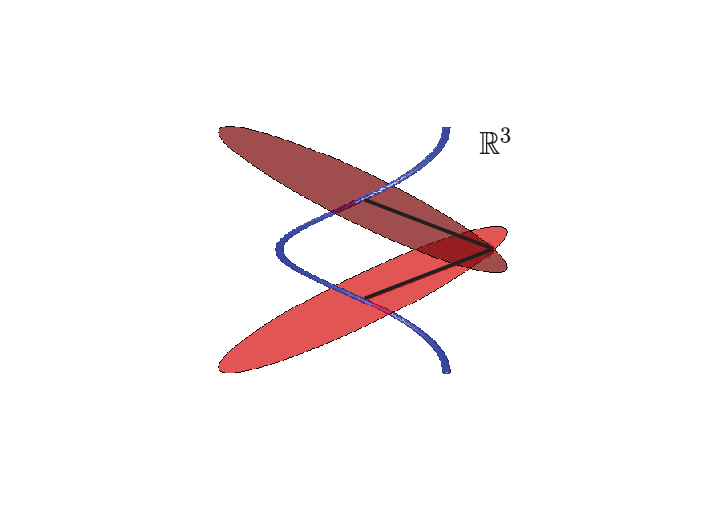
This result states that for general manifolds, the most we can say is that the condition number of the joint manifold is guaranteed to be less than that of the worst manifold. However, in practice this is not likely to happen. As an example, Figure 2 illustrates the point at which the normal bundle intersects itself for the case of the joint manifold from Figure 1 (c). In this case we obtain $\tau^{*}=\sqrt{\pi^{2}/2+1}$ . Note that the condition numbers for the manifolds ${\mathcal{M}}_{1}$ and ${\mathcal{M}}_{2}$ generating ${\mathcal{M}}^{*}$ are given by $\tau_{1}=\infty$ and $\tau_{2}=1$ . Thus, while the condition number in this case is not as good as the best manifold, it is still notably better than the worst manifold. In general, even this example may be somewhat pessimistic, and it is possible that in many cases the joint manifold may be better conditioned than even the best manifold.

3 Joint manifolds in signal processing

Manifold models can be exploited by a number of algorithms for signal processing tasks such as pattern classification, learning, and control [11]. The performance of such algorithms often depends on geometric properties of the manifold model such as its condition number and geodesic distances along its surface. The theory developed in Section 2 suggests that the joint manifold preserves or improves these properties. We will now see that when noise is introduced these results suggest that, in the case of multiple data sources, it can be extremely beneficial to use algorithms specifically designed to exploit the joint manifold structure.

3.1 Classification

We first study the problem of manifold-based classification. The problem is defined as follows: given manifolds ${\mathcal{M}}$ and ${\mathcal{N}}$ , suppose we observe a signal $y=x+n\in\mathbb{R}^{N}$ where either $x\in{\mathcal{M}}$ or $x\in{\mathcal{N}}$ and $n$ is a noise vector, and we wish to find a function $f:\mathbb{R}^{N}\rightarrow\{{\mathcal{M}},{\mathcal{N}}\}$ that attempts to determine which manifold “generated” $y$ . We consider a simple classification algorithm based on the generalized maximum likelihood framework described in [12]. The approach is to classify by computing the distance from the observed signal $y$ to each of the manifolds, and then classify based on which of these distances is smallest, i.e., our classifier is

f(y)=\arg\min\left[d(y,{\mathcal{M}}),d(y,{\mathcal{N}})\right].

(9)

We will measure the performance of this algorithm for a particular pair of manifolds by considering the probability of misclassifying a point from ${\mathcal{M}}$ as belonging to ${\mathcal{N}}$ , which we denote $P_{{\mathcal{M}}{\mathcal{N}}}$ .

To analyze this problem, we employ three common notions of separation in metric spaces:

•

The minimum separation distance between two manifolds ${\mathcal{M}}$ and ${\mathcal{N}}$ is defined as

$\delta({\mathcal{M}},{\mathcal{N}})=\inf_{p\in{\mathcal{M}}}d(p,{\mathcal{N}}).$
•

The Hausdorff distance from ${\mathcal{M}}$ to ${\mathcal{N}}$ is defined to be

$D({\mathcal{M}},{\mathcal{N}})=\sup_{p\in{\mathcal{M}}}d(p,{\mathcal{N}}),$

with $D({\mathcal{N}},{\mathcal{M}})$ defined similarly. Note that $\delta({\mathcal{M}},{\mathcal{N}})=\delta({\mathcal{N}},{\mathcal{M}})$ , while in general
$D({\mathcal{M}},{\mathcal{N}})\neq D({\mathcal{N}},{\mathcal{M}})$ .
•

The maximum separation distance between manifolds ${\mathcal{M}}$ and ${\mathcal{N}}$ is defined as

$\Delta({\mathcal{M}},{\mathcal{N}})=\sup_{x\in{\mathcal{M}}}\sup_{y\in{\mathcal{N}}}\|x-y\|.$

As one might expect, $P_{{\mathcal{M}}{\mathcal{N}}}$ is controlled by the separation distances. For example, suppose that $x\in{\mathcal{M}}$ ; if the noise vector $n$ is bounded and satisfies $\|n\|<\delta({\mathcal{M}},{\mathcal{N}})/2$ , then we have that $d(y,{\mathcal{M}})\leq\|n\|<\delta({\mathcal{M}},{\mathcal{N}})/2$ and hence

$\displaystyle\delta({\mathcal{M}},{\mathcal{N}})$	$\displaystyle=$	$\displaystyle\inf_{p\in{\mathcal{M}},q\in{\mathcal{N}}}\\|p-q\\|$
	$\displaystyle=$	$\displaystyle\inf_{p\in{\mathcal{M}},q\in{\mathcal{N}}}\\|p-y+y-q\\|$
	$\displaystyle\leq$	$\displaystyle\inf_{p\in{\mathcal{M}},q\in{\mathcal{N}}}\\|p-y\\|+\\|y-q\\|$
	$\displaystyle=$	$\displaystyle d(y,{\mathcal{M}})+d(y,{\mathcal{N}})$
	$\displaystyle<$	$\displaystyle\delta({\mathcal{M}},{\mathcal{N}})/2+d(y,{\mathcal{N}}).$

Thus we are guaranteed that

d(y,{\mathcal{N}})>\delta({\mathcal{M}},{\mathcal{N}})/2.

Therefore, $d(y,{\mathcal{M}})<d(y,{\mathcal{N}})$ and the classifier defined by (9) satisfies $P_{{\mathcal{M}}{\mathcal{N}}}=0$ . We can refine this result in two possible ways. First, note that the amount of noise $\epsilon$ that we can tolerate without making an error depends on $x$ . Specifically, for a given $x\in{\mathcal{M}}$ , provided that $\|n\|\leq d(x,{\mathcal{N}})/2$ we still have that $P_{{\mathcal{M}}{\mathcal{N}}}=0$ . Thus, for a given $x\in{\mathcal{M}}$ we can tolerate noise bounded by $d(x,{\mathcal{N}})/2\in[\delta({\mathcal{M}},{\mathcal{N}})/2,D({\mathcal{M}},{\mathcal{N}})/2]$ .

A second possible refinement that we will explore below is to ignore this dependence of $x$ , but to extend our noise model to the case where $\|n\|>\delta({\mathcal{M}},{\mathcal{N}})/2$ with non-zero probability. We can still bound $P_{{\mathcal{M}}{\mathcal{N}}}$ since

P_{{\mathcal{M}}{\mathcal{N}}}\leq P(\|n\|>\delta({\mathcal{M}},{\mathcal{N}})/2).

(10)

We provide bounds on this probability for both the component manifolds and the joint manifold as follows: first, we first compare the separation distances for these cases.

Theorem 3.1.

Consider the joint manifolds ${\mathcal{M}}^{*}\subset{\mathcal{M}}_{1}\times{\mathcal{M}}_{2}\times\cdots\times{\mathcal{M}}_{J}$ and ${\mathcal{N}}^{*}\subset{\mathcal{N}}_{1}\times{\mathcal{N}}_{2}\times\cdots\times{\mathcal{N}}_{J}$ . Then, the following bounds hold:

Joint minimum separation:

\sum_{j=1}^{J}\delta^{2}({\mathcal{M}}_{j},{\mathcal{N}}_{j})\leq\delta^{2}({\mathcal{M}}^{*},{\mathcal{N}}^{*})\leq\min_{1\leq k\leq J}\left(\delta^{2}({\mathcal{M}}_{k},{\mathcal{N}}_{k})+\sum_{j\neq k}\Delta^{2}({\mathcal{M}}_{j},{\mathcal{N}}_{j})\right).

(11)

Joint Hausdorff separation from ${\mathcal{M}}^{*}$ to ${\mathcal{N}}^{*}$ :

\max_{1\leq k\leq J}\left(D^{2}({\mathcal{M}}_{k},{\mathcal{N}}_{k})+\sum_{j\neq k}\delta^{2}({\mathcal{M}}_{j},{\mathcal{N}}_{j})\right)\leq D^{2}({\mathcal{M}}^{*},{\mathcal{N}}^{*})\leq\sum_{j=1}^{J}\Delta^{2}({\mathcal{M}}_{j},{\mathcal{N}}_{j}).

(12)

Joint maximum separation from ${\mathcal{M}}^{*}$ to ${\mathcal{N}}^{*}$ :

\max_{1\leq k\leq J}\left(\Delta^{2}({\mathcal{M}}_{k},{\mathcal{N}}_{k})+\sum_{j\neq k}\delta^{2}({\mathcal{M}}_{j},{\mathcal{N}}_{j})\right)\leq\Delta^{2}({\mathcal{M}}^{*},{\mathcal{N}}^{*})\leq\sum_{j=1}^{J}\Delta^{2}({\mathcal{M}}_{j},{\mathcal{N}}_{j}).

(13)

Proof.

Inequality (11) is a simple corollary of Proposition 2.3. Let $p=(p_{1},p_{2},\ldots,p_{J})$ and $q=(q_{1},q_{2},\ldots,q_{J})$ respectively be the points on ${\mathcal{M}}^{*}$ and ${\mathcal{N}}^{*}$ for which the minimum separation distance $\delta({\mathcal{M}}^{*},{\mathcal{N}}^{*})$ is attained, i.e.,

(p,q)=\arg\inf_{p\in{\mathcal{M}}^{*}}\inf_{q\in{\mathcal{N}}^{*}}\|p-q\|.

Then,

	$\displaystyle\delta^{2}({\mathcal{M}}^{},{\mathcal{N}}^{})$	$\displaystyle=$	$\displaystyle\\|p-q\\|^{2}=\sum_{j=1}^{J}\\|p_{j}-q_{j}\\|^{2}$
		$\displaystyle\geq$	$\displaystyle\sum_{j=1}^{J}\delta^{2}({\mathcal{M}}_{j},{\mathcal{N}}_{j}),$

since the distance between two points in any given component space is greater than the minimum separation distance corresponding to that space. This establishes the lower bound in (11). We obtain the upper bound by selecting a $k$ , and selecting $p\in{\mathcal{M}}^{*}$ and $q\in{\mathcal{N}}^{*}$ such that $p_{k}$ and $q_{k}$ attain the minimum separation distance $\delta({\mathcal{M}}_{k},{\mathcal{N}}_{k})$ . From the definition of $\delta({\mathcal{M}}^{*},{\mathcal{N}}^{*})$ , we have that

$\displaystyle\delta^{2}({\mathcal{M}}^{},{\mathcal{N}}^{})$	$\displaystyle\leq$	$\displaystyle\\|p-q\\|^{2}=\sum_{j=1}^{J}\\|p_{j}-q_{j}\\|^{2}$
	$\displaystyle=$	$\displaystyle\delta^{2}({\mathcal{M}}_{k},{\mathcal{N}}_{k})+\sum_{j\neq k}\\|p_{j}-q_{j}\\|^{2}$
	$\displaystyle\leq$	$\displaystyle\delta^{2}({\mathcal{M}}_{k},{\mathcal{N}}_{k})+\sum_{j\neq k}\Delta^{2}({\mathcal{M}}_{j},{\mathcal{N}}_{j}),$

and since this holds for every choice of $k$ , (11) follows by taking the minimum over all $k$ .

To prove inequality (12), we follow a similar course. We begin by selecting $p\in{\mathcal{M}}^{*}$ and $q\in{\mathcal{N}}^{*}$ that satisfy

(p,q)=\arg\sup_{p\in{\mathcal{M}}^{*}}\inf_{q\in{\mathcal{N}}^{*}}\|p-q\|.

Then,

	$\displaystyle D^{2}({\mathcal{M}}^{},{\mathcal{N}}^{})$	$\displaystyle=$	$\displaystyle\\|p-q\\|^{2}=\sum_{j=1}^{J}\\|p_{j}-q_{j}\\|^{2}$
		$\displaystyle\leq$	$\displaystyle\sum_{j=1}^{J}\Delta^{2}({\mathcal{M}}_{j},{\mathcal{N}}_{j}),$

which establishes the upper bound in (12). To obtain the lower bound, we again select a $k$ , and now let $p\in{\mathcal{M}}^{*}$ be the point for which the corresponding at which the Hausdorff separation for the component manifold ${\mathcal{M}}_{k}$ is attained, i.e., the corresponding point $p_{k}$ is furthest away from ${\mathcal{N}}_{k}$ as can be possible in ${\mathcal{M}}_{k}$ . Let $q\in{\mathcal{N}}^{*}$ be the nearest point in ${\mathcal{N}}^{*}$ to $p$ . From the definition of the Hausdorff distance, we get that

D({\mathcal{M}}^{*},{\mathcal{N}}^{*})\geq\|p-q\|,

since the Hausdorff distance is the maximal distance between the points in ${\mathcal{M}}^{*}$ and their respective nearest neighbors in ${\mathcal{N}}^{*}$ . Again, it also follows that

$\displaystyle D^{2}({\mathcal{M}}^{},{\mathcal{N}}^{})$	$\displaystyle\geq$	$\displaystyle\\|p-q\\|^{2}=\\|p_{k}-q_{k}\\|^{2}+\sum_{j\neq k}\\|p_{j}-q_{j}\\|^{2}$
	$\displaystyle=$	$\displaystyle D^{2}({\mathcal{M}}_{k},{\mathcal{N}}_{k})+\sum_{j\neq k}\\|p_{j}-q_{j}\\|^{2}$
	$\displaystyle\geq$	$\displaystyle D^{2}({\mathcal{M}}_{k},{\mathcal{N}}_{k})+\sum_{j\neq k}\delta^{2}({\mathcal{M}}_{j},{\mathcal{N}}_{j}).$

Since this again holds for every choice of $k$ , (12) follows by taking the maximum over all $k$ .

One can prove (13) using the same technique used to prove (12). ∎

As an example, if we consider the case where the separation distances are constant for all $j$ , then the joint minimum separation distance satisfies

	$\displaystyle\sqrt{J}\delta({\mathcal{M}}_{1},{\mathcal{N}}_{1})\leq\delta({\mathcal{M}}^{},{\mathcal{N}}^{})$	$\displaystyle\leq$	$\displaystyle\sqrt{\delta^{2}({\mathcal{M}}_{1},{\mathcal{N}}_{1})+(J-1)\Delta^{2}({\mathcal{M}}_{1},{\mathcal{N}}_{1})}$
		$\displaystyle\leq$	$\displaystyle\delta({\mathcal{M}}_{1},{\mathcal{N}}_{1})+\sqrt{J-1}\Delta({\mathcal{M}}_{1},{\mathcal{N}}_{1})$

In the case where $\delta({\mathcal{M}}_{1},{\mathcal{N}}_{1})\ll\Delta({\mathcal{M}}_{1},{\mathcal{N}}_{1})$ then we observe that $\delta({\mathcal{M}}^{*},{\mathcal{N}}^{*})$ can be considerably larger than $\sqrt{J}\delta({\mathcal{M}}_{1},{\mathcal{N}}_{1})$ . This means that we can potentially tolerate much more noise while ensuring $P_{{\mathcal{M}}^{*}{\mathcal{N}}^{*}}=0$ . To see this, write $n=(n_{1},n_{2},\ldots,n_{J})$ and recall that we require $\|n_{j}\|<\epsilon=\delta({\mathcal{M}}_{j},{\mathcal{N}}_{j})/2$ to ensure that $P_{{\mathcal{M}}_{j}{\mathcal{N}}_{j}}=0$ . Thus, if we require that $P_{{\mathcal{M}}_{j}{\mathcal{N}}_{j}}=0$ for all $j$ , then we have that

\|n\|=\sqrt{\sum_{j=1}^{J}\|n_{j}\|^{2}}<\sqrt{J}\epsilon=\sqrt{J}\delta({\mathcal{M}}_{1},{\mathcal{N}}_{1})/2.

However, if we instead only require that $P_{{\mathcal{M}}^{*}{\mathcal{N}}^{*}}=0$ we only need $\|n\|<\delta({\mathcal{M}}^{*},{\mathcal{N}}^{*})/2$ , which can be a significantly less stringent requirement.

The benefit of classification using the joint manifold is made more apparent when we extend our noise model to the case where we allow $\|n_{j}\|>\delta({\mathcal{M}}_{j},{\mathcal{N}}_{j})/2$ with non-zero probability and apply (10). To bound the probability in (10), we will make use of the following adaptation of Hoeffding’s inequality [13].

Lemma 3.1.

Suppose that $n_{j}\in\mathbb{R}^{N}$ is a random vector that satisfies $\|n_{j}\|\leq\epsilon$ , for $j=1,2,\ldots,J$ . Suppose also that the $n_{j}$ are independent and identically distributed (i.i.d.) with $E[\|n_{j}\|]=\sigma$ . Then if $n=(n_{1},n_{2},\ldots,n_{J})\in\mathbb{R}^{JN}$ , we have that for any $\lambda>0$ ,

P\left(\|n\|^{2}>J(\sigma^{2}+\lambda)\right)\leq\exp\left(-\frac{2J\lambda^{2}}{\epsilon^{4}}\right).

Using this lemma we can relax the assumption on $\epsilon$ so that we only require that it is finite, and instead make the weaker assumption that $E[\|n\|]=\sqrt{J}\sigma\leq\delta({\mathcal{M}},{\mathcal{N}})/2$ for a particular pair of manifolds ${\mathcal{M}}$ , ${\mathcal{N}}$ . This assumption ensures that $\lambda=\delta^{2}({\mathcal{M}},{\mathcal{N}})/4-\sigma^{2}>0$ , so that we can combine Lemma 3.1 with (10) to obtain a bound on $P_{{\mathcal{M}}{\mathcal{N}}}$ . Note that if this condition does not hold, then this is a very difficult classification problem since the expected norm of the noise is large enough to push us closer to the other manifold, in which case the simple classifier given by (9) makes little sense.

We now illustrate how Lemma 3.1 can be be used to compare error bounds between classification using a joint manifold and classification using a particular pair of component manifolds ${\mathcal{M}}_{k},{\mathcal{N}}_{k}$ .

Theorem 3.2.

Suppose that we observe a vector $y=x+n$ where $x\in{\mathcal{M}}^{*}$ and $n=(n_{1},n_{2},\ldots,n_{J})$ is a random vector such that $\|n_{j}\|\leq\epsilon$ , for $j=1,2,\ldots,J$ , and that the $n_{j}$ are i.i.d. with $E[\|n_{j}\|]=\sigma\leq\delta({\mathcal{M}}_{k},{\mathcal{N}}_{k})/2$ . If

\delta({\mathcal{M}}_{k},{\mathcal{N}}_{k})\leq\frac{\delta({\mathcal{M}}^{*},{\mathcal{N}}^{*})}{\sqrt{J}},

(14)

and we classify the observation $y$ according to (9), then

P_{{\mathcal{M}}^{*}{\mathcal{N}}^{*}}\leq\exp\left(-\frac{2c^{*}}{\epsilon^{4}}\right),

(15)

and

P_{{\mathcal{M}}_{k}{\mathcal{N}}_{k}}\leq\exp\left(-\frac{2c_{k}}{\epsilon^{4}}\right),

(16)

such that

c^{*}>c_{k}.

Proof.

First, observe that

\frac{\delta^{2}({\mathcal{M}}^{*},{\mathcal{N}}^{*})}{J}\geq\delta^{2}({\mathcal{M}}_{k},{\mathcal{N}}_{k})\geq 4\sigma^{2}.

(17)

Thus, we may set $\lambda=\delta^{2}({\mathcal{M}}^{*},{\mathcal{N}}^{*})/4J-\sigma^{2}>0$ and apply Lemma 3.1 to obtain (15) with

c^{*}=J\left(\frac{\delta^{2}({\mathcal{M}}^{*},{\mathcal{N}}^{*})}{4J}-\sigma^{2}\right)^{2}.

Similarly, we may again apply Lemma 3.1 by setting $\lambda=\delta^{2}({\mathcal{M}}_{j},{\mathcal{N}}_{j})/4-\sigma^{2}>0$ and $J=1$ to obtain (16) with

c_{k}=\left(\frac{\delta^{2}({\mathcal{M}}_{k},{\mathcal{N}}_{k})}{4}-\sigma^{2}\right)^{2}.

It remains to show that $c^{*}>c_{k}$ . Thus, observe that

$\displaystyle\delta^{2}({\mathcal{M}}_{k},{\mathcal{N}}_{k})$	$\displaystyle\leq$	$\displaystyle\frac{\delta^{2}({\mathcal{M}}^{},{\mathcal{N}}^{})}{J}$
	$\displaystyle=$	$\displaystyle\frac{\sqrt{J}\delta^{2}({\mathcal{M}}^{},{\mathcal{N}}^{})-(\sqrt{J}-1)\delta^{2}({\mathcal{M}}^{},{\mathcal{N}}^{})}{J}$
	$\displaystyle=$	$\displaystyle\frac{\delta^{2}({\mathcal{M}}^{},{\mathcal{N}}^{})}{\sqrt{J}}-(\sqrt{J}-1)\frac{\delta^{2}({\mathcal{M}}^{},{\mathcal{N}}^{})}{J}$
	$\displaystyle\leq$	$\displaystyle\frac{\delta^{2}({\mathcal{M}}^{},{\mathcal{N}}^{})}{\sqrt{J}}-4\sigma^{2}(\sqrt{J}-1),$

where the last inequality follows from (17). Rearranging terms, we obtain

\frac{\delta^{2}({\mathcal{M}}_{k},{\mathcal{N}}_{k})}{4}-\sigma^{2}\leq\sqrt{J}\left(\frac{\delta^{2}({\mathcal{M}}^{*},{\mathcal{N}}^{*})}{4J}-\sigma^{2}\right).

Thus,

\sqrt{c_{k}}\leq\sqrt{c^{*}},

and since $c_{k}>0$ by assumption, we obtain

c_{k}\leq c^{*},

as desired. ∎

This result can be weakened slightly to obtain the following corollary.

Corollary 3.1.

Suppose that we observe a vector $y=x+n$ where $x\in{\mathcal{M}}^{*}$ and $n=(n_{1},n_{2},\ldots,n_{J})$ is a random vector such that $\|n_{j}\|\leq\epsilon$ , for $j=1,2,\ldots,J$ and that the $n_{j}$ are i.i.d. with $E[\|n_{j}\|]=\sigma\leq\delta({\mathcal{M}}_{k},{\mathcal{N}}_{k})/2$ . If

\delta^{2}({\mathcal{M}}_{k},{\mathcal{N}}_{k})\leq\frac{\sum_{j\neq k}\delta^{2}({\mathcal{M}}_{j},{\mathcal{N}}_{j})}{J-1},

(18)

and we classify according to (9), then (15) and (16) hold with the same constants as in Theorem 3.2.

Proof.

We can rewrite (18) as

\delta^{2}({\mathcal{M}}_{k},{\mathcal{N}}_{k})\leq\frac{\sum_{j=1}^{J}\delta^{2}({\mathcal{M}}_{j},{\mathcal{N}}_{j})-\delta^{2}({\mathcal{M}}_{k},{\mathcal{N}}_{k})}{J-1}.

After rearranging terms, this reduces to

\delta^{2}({\mathcal{M}}_{k},{\mathcal{N}}_{k})\leq\frac{\sum_{j=1}^{J}\delta^{2}({\mathcal{M}}_{j},{\mathcal{N}}_{j})}{J}.

Applying (11) from Theorem 3.1, we obtain

\delta^{2}({\mathcal{M}}_{k},{\mathcal{N}}_{k})\leq\frac{\delta^{2}({\mathcal{M}}^{*},{\mathcal{N}}^{*})}{J},

which allows us to apply Theorem 3.2 to prove the desired result. ∎

Corollary 3.1 shows that we can expect joint classification to outperform the $k$ -th individual classifier whenever the squared separation distance for the $k$ -th component manifolds is not too much larger than the average squared separation distance among the remaining component manifolds. Thus, we can expect that the joint classifier is outperforming most of the individual classifiers, but it is still possible that some of the individual classifiers are doing better. Of course, if one were able to know in advance which classifiers were best, then one would only use data from the best sensors. We expect that a more typical situation is when the separation distances are (approximately) equal across all sensors, in which case the condition in (18) is true for all of the component manifolds.

3.2 Manifold learning

In contrast to the classification scenario described above, where we knew the manifold structure a priori, we now consider manifold learning algorithms that attempt to learn the manifold structure by constructing a (possibly nonlinear) embedding of a given point cloud into a subset of $\mathbb{R}^{L}$ , where $L<N$ . Typically, $L$ is set to $K$ , the intrinsic manifold dimension. Several such algorithms have been proposed, each giving rise to a nonlinear map with its own special properties and advantages (e.g. Isomap [14], Locally Linear Embedding (LLE) [15], Hessian Eigenmaps [16], etc.) Such algorithms provide a powerful framework for navigation, visualization and interpolation of high-dimensional data. For instance, manifold learning can be employed in the inference of articulation parameters (eg., 3-D pose) of points sampled from an image appearance manifold.

In particular, the Isomap algorithm deserves special mention. It assumes that the point cloud consists of samples from a data manifold that is (at least approximately) isometric to a convex subset of Euclidean space. In this case, there exists an isometric mapping $f$ from a parameter space $\Theta\subseteq\mathbb{R}^{K}$ to the manifold ${\mathcal{M}}$ such that the geodesic distance between every pair of data points is equal to the $\ell_{2}$ distance between their corresponding pre-images in $\Theta$ . In essence, Isomap attempts to discover the coordinate structure of that $K$ -dimensional space.

Isomap works in three stages:

•

We construct a graph $G$ that contains one vertex for each input data point; an edge connects two vertices if the Euclidean distance between the corresponding data points is below a specified threshold.
•

We weight each edge in the graph $G$ by computing the Euclidean distance between the corresponding data points. We then estimate the geodesic distance between each pair of vertices as the length of the shortest path between the corresponding vertices in the graph $G$ .
•

We embed the points in $\mathbb{R}^{K}$ using multidimensional scaling (MDS), which attempts to embed the points so that their Euclidean distance approximates the geodesic distances estimated in the previous step.

A crucial component of the MDS algorithm is a suitable linear transformation of the matrix of squared geodesic distances $D$ ; the rank- $K$ approximation of this new matrix yields the best possible $K$ -dimensional coordinate structure of the input sample points in a mean-squared sense. Further results on the performance of Isomap in terms of geometric properties of the underlying manifold can be found in [17].

We examine the performance of manifold learning using Isomap with samples of the joint manifold, as compared to learning any of the component manifolds. We first assume that we are given noiseless samples from the $J$ isometric component manifolds ${\mathcal{M}}_{1},{\mathcal{M}}_{2},\ldots,{\mathcal{M}}_{J}$ . In order to judge the quality of the embedding learned by the Isomap algorithm, we will observe that for any pair of points $p,q$ on a manifold ${\mathcal{M}}$ , we have that

\rho\leq\frac{\|p-q\|}{d_{\mathcal{M}}(p,q)}\leq 1

(19)

for some $\rho\in[0,1]$ that will depend on $p,q$ . Isomap will perform well if the largest value of $\rho$ that satisfies (19) for any pair of samples that are connected by an edge in the graph $G$ is close to $1$ . Using this result, we can compare the performance of manifold learning using Isomap on samples from the joint manifold ${\mathcal{M}}^{*}$ to using Isomap on samples from a particular component manifold ${\mathcal{M}}_{k}$ .

Theorem 3.3.

Let ${\mathcal{M}}^{*}$ be a joint manifold from $J$ isometric component manifolds. Let $p=(p_{1},p_{2},\ldots,p_{J})$ and $q=(q_{1},q_{2},\ldots,q_{J})$ denote a pair of samples of ${\mathcal{M}}^{*}$ and suppose that we are given a graph $G$ that contains one vertex for each sample. For each $k=1,\ldots,J$ , define $\rho_{j}$ as the largest value such that

\rho_{j}\leq\frac{\|p_{j}-q_{j}\|}{d_{{\mathcal{M}}_{j}}(p_{j},q_{j})}\leq 1

(20)

for all pairs of points connected by an edge in $G$ . Then we have that

\sqrt{\frac{\sum_{j=1}^{J}\rho_{j}^{2}}{J}}\leq\frac{\|p-q\|}{d_{{\mathcal{M}}^{*}}(p,q)}\leq 1.

(21)

Proof.

By Proposition 2.3,

\|p-q\|^{2}=\sum_{j=1}^{J}\|p_{j}-q_{j}\|^{2},

and from Theorem 2.1 we have that

d_{{\mathcal{M}}^{*}}^{2}(p,q)=Jd_{{\mathcal{M}}_{1}}^{2}(p_{1},q_{1}).

Thus,

$\displaystyle\frac{\\|p-q\\|^{2}}{d_{{\mathcal{M}}^{*}}^{2}(p,q)}$	$\displaystyle=$	$\displaystyle\frac{\sum_{j=1}^{J}\\|p_{j}-q_{j}\\|^{2}}{Jd_{{\mathcal{M}}_{1}}^{2}(p_{1},q_{1})}$
	$\displaystyle=$	$\displaystyle\frac{1}{J}\sum_{j=1}^{J}\frac{\\|p_{j}-q_{j}\\|^{2}}{d_{{\mathcal{M}}_{1}}^{2}(p_{1},q_{1})}$
	$\displaystyle=$	$\displaystyle\frac{1}{J}\sum_{j=1}^{J}\frac{\\|p_{j}-q_{j}\\|^{2}}{d_{{\mathcal{M}}_{j}}^{2}(p_{j},q_{j})}$
	$\displaystyle\geq$	$\displaystyle\frac{1}{J}\sum_{j=1}^{J}\rho_{j}^{2},$

which establishes the lower bound in (21). The upper bound is trivial since we always have that $d_{{\mathcal{M}}^{*}}(p,q)\geq\|p-q\|$ . ∎

From Theorem 3.3 we see that, in many cases, the joint manifold estimates of the geodesic distances will be more accurate than the estimates obtained using one of the component manifolds. For instance, if for particular component manifold ${\mathcal{M}}_{k}$ we observe that

\rho_{k}\leq\sqrt{\frac{\sum_{j=1}^{J}\rho_{j}^{2}}{J}},

then we know that the joint manifold leads to better estimates. Essentially, we can expect that the joint manifold will lead to estimates that are better than the average case across the component manifolds.

We now consider the case where we have a sufficiently dense sampling of the manifolds so that the $\rho_{j}$ are very close to one, and examine the case where we are obtaining noisy samples. We will assume that the noise affecting the data samples is i.i.d., and demonstrate that any distance calculation performed on ${\mathcal{M}}^{*}$ serves as a better estimator of the pairwise (and consequently, geodesic) distances between two points labeled by $p$ and $q$ than that performed on any component manifold between their corresponding points $p_{j}$ and $q_{j}$ .

Theorem 3.4.

Let ${\mathcal{M}}^{*}$ be a joint manifold from $J$ isometric component manifolds. Let $p=(p_{1},p_{2},\ldots,p_{J})$ and $q=(q_{1},q_{2},\ldots,q_{J})$ be samples of ${\mathcal{M}}^{*}$ and assume that $\|p_{j}-q_{j}\|=d$ for all $j$ . Assume that we acquire noisy observations $s=p+n$ and $r=q+n^{\prime}$ , where $n=(n_{1},n_{2},\ldots,n_{J})$ and $n^{\prime}=(n^{\prime}_{1},n^{\prime}_{2},\ldots,n^{\prime}_{J})$ are independent noise vectors with the same variance and norm bound

\mathbb{E}[\|n_{j}\|^{2}]=\sigma^{2}~~\textrm{and}~~\|n_{j}\|^{2}\leq\epsilon,~~j=1,\ldots,J.

Then,

P\left(1-\delta\leq\frac{\|s-r\|^{2}}{\|p-q\|^{2}+2J\sigma^{2}}\leq 1+\delta\right)\geq 1-2c^{-{J^{2}}},

where $c=\mathrm{exp}\left(2\delta^{2}\left(\frac{d^{2}+2\sigma^{2}}{d\sqrt{\epsilon}+\epsilon}\right)^{2}\right)$ .

Proof.

We write the distance between the noisy samples as

\|s-r\|^{2}=\sum_{j=1}^{J}\{{\|p_{j}-q_{j}\|^{2}+2\langle p_{j}-q_{j},n_{j}-n^{\prime}_{j}\rangle+\|n_{j}-n^{\prime}_{j}\|^{2}}\}.

(22)

This can be rewritten as

\|s-r\|^{2}-\|p-q\|^{2}=\sum_{j=1}^{J}\{{2\langle p_{j}-q_{j},n_{j}-n^{\prime}_{j}\rangle+\|n_{j}-n^{\prime}_{j}\|^{2}}\}.

(23)

We obtain the following statistics for the term inside the sum:

	$\displaystyle\mathbb{E}[\langle p_{j}-q_{j},n_{j}-n^{\prime}_{j}\rangle+\\|n_{j}-n^{\prime}_{j}\\|^{2}]$	$\displaystyle=$	$\displaystyle 2\sigma^{2},$
	$\displaystyle\left\|\langle p_{j}-q_{j},n_{j}-n^{\prime}_{j}\rangle+\\|n_{j}-n^{\prime}_{j}\\|^{2}\right\|$	$\displaystyle\leq$	$\displaystyle 2d\sqrt{\epsilon}+\epsilon.$

Using Hoeffding’s inequality, we obtain

P\left(\left|\sum_{j=1}^{J}\{{2\langle p_{j}-q_{j},n_{j}-n^{\prime}_{j}\rangle+\|n_{j}-n^{\prime}_{j}\|^{2}}\}-2J\sigma^{2}\right|>J^{2}\lambda\right)\leq 2e^{-\frac{2J\lambda^{2}}{(2d\sqrt{\epsilon}+\epsilon)^{2}}}.

This result is rewritten to obtain

	$\displaystyle P\left(\left\|\\|s-r\\|^{2}-\\|p-q\\|^{2}-2J\sigma^{2}\right\|>J\lambda\right)$	$\displaystyle\leq$	$\displaystyle 2e^{-\frac{2J^{2}\lambda^{2}}{(2d\sqrt{\epsilon}+\epsilon)^{2}}},$
	$\displaystyle P\left(\left\|\\|s-r\\|^{2}-\\|p-q\\|^{2}-2J\sigma^{2}\right\|\leq J\lambda\right)$	$\displaystyle\geq$	$\displaystyle 1-2e^{-\frac{2J^{2}\lambda^{2}}{(2d\sqrt{\epsilon}+\epsilon)^{2}}}.$

Simplifying, we get

P\left(1-\frac{\lambda}{d^{2}+2\sigma^{2}}\leq\frac{\|s-r\|^{2}}{\|p-q\|^{2}+2J\sigma^{2}}\leq 1+\frac{\lambda}{d^{2}+2\sigma^{2}}\right)\geq 1-2e^{-\frac{2J^{2}\lambda^{2}}{(2d\sqrt{\epsilon}+\epsilon)^{2}}}.

Replace $\delta=\frac{\lambda}{d^{2}+2\sigma^{2}}$ to obtain the result. ∎

We observe that the estimate of the true distance suffers from a constant small bias; this can be handled using a simple debiasing step.²² 2 Manifold learning algorithms such as Isomap deal with biased estimates of distances by “centering” the matrix of squared distances, i.e., removing the mean of each row/column from every element. Theorem 3.4 indicates that the probability of large deviations in the estimated distance decreases exponentially in the number of component manifolds $J$ ; thus the “denoising” effect in joint manifold learning is manifested even in the case where only a small number of component manifolds are present.

As an example, we consider three different manifolds formed by images of an ellipse with major axis $a$ and minor axis $b$ translating in a 2-D plane; an example point is shown in Figure 3. The eccentricity of the ellipse directly affects the condition number $1/\tau$ of the image articulation manifold; in fact, it can be shown that articulation manifolds formed by more eccentric ellipses exhibit higher values for the condition number. Consequently, we expect that it is “harder” to learn such manifolds.

Figure 4 shows that this is indeed the case. We add a small amount of white gaussian noise to each image and apply the Isomap algorithm [14] to both the individual datasets as well as the concatenated dataset. We observe that the 2-D embedding is poorly learnt in each of the individual manifolds, but improves visibly when the data ensemble is modeled using a joint manifold.

4 Joint manifolds for efficient dimensionality reduction

We have shown that joint manifold models for data ensembles can significantly improve the performance on a variety of signal processing tasks, where performance is quantified using metrics like probability of error for detection and accuracy for parameter estimation and manifold learning. In particular, we have observed that performance tends to improve exponentially fast as we increase the number of component manifolds $J$ . However, we have ignored that when $J$ and the ambient dimension of the manifolds $N$ become large, the dimensionality of the joint manifold — $JN$ — may be so large that it becomes impossible to perform any meaningful computations. Fortunately, we can transform the data into a more amenable form via the method of random projections: it has been shown that the essential structure of a $K$ -dimensional manifold with condition number $1/\tau$ residing in $\mathbb{R}^{N}$ is approximately preserved under an orthogonal projection into a random subspace of dimension $O(K\log(N/\tau))\ll N$ [18]. This result can be leveraged to enable efficient design of inference applications, such as classification using multiscale navigation [19], intrinsic dimension estimation, and manifold learning [20].

We can apply this result individually for each sensor acquiring manifold-modeled data. Suppose $N$ -dimensional data from $J$ component manifolds is available. If $N$ is large, then the above result would suggest that we project each manifold into a lower-dimensional subspace. By collecting this data at a central location, we would obtain $J$ vectors, each of dimension $O(K\log N)$ , so that we would have $O(JK\log N)$ total measurements. This approach, however, essentially ignores the joint manifold structure present in the data. If we instead view the data as arising from a $K$ -dimensional joint manifold residing in $\mathbb{R}^{JN}$ with bounded condition number as given by Theorem 2.2, we can then project the joint data into a subspace which is only logarithmic in $J$ as well as the largest condition number among the components, and still approximately preserve the manifold structure. This is formalized in the following theorem.

Theorem 4.1.

Let ${\mathcal{M}}^{*}$ be a compact, smooth, Riemannian joint manifold in a $JN$ -dimensional space with condition number $1/\tau^{*}$ . Let $\Phi$ denote an orthogonal linear mapping from ${\mathcal{M}}^{*}$ into a random $M$ -dimensional subspace of $\mathbb{R}^{JN}$ . Let $M\geq O(K\log(JN/\tau^{*})/\epsilon^{2})$ . Then, with high probability, the geodesic and Euclidean distances between any pair of points on ${\mathcal{M}}^{*}$ are preserved up to distortion $\epsilon$ under the linear transformation $\Phi$ .

Thus, we obtain a faithful approximation of our manifold-modeled data that is only $O(K\log JN)$ dimensional. This represents a significant improvement over performing separate dimensionality reduction on each component manifold.

Importantly, the linear nature of the random projection step can be utilized to perform dimensionality reduction in a distributed manner, which is particularly useful in applications when data transmission is expensive. As an example, consider a network of $J$ sensors observing an event that is governed by a $K$ -dimensional parameter. Each sensor records a signal $x_{j}\in\mathbb{R}^{N},1\ \leq j\leq J$ ; the concatenation of the signals $x=[x_{1}^{T}~x_{2}^{T}~\ldots~x_{j}^{T}]^{T}$ lies on a $K$ -dimensional joint manifold ${\mathcal{M}}^{*}\subset\mathbb{R}^{JN}$ . Since the required random projections are linear, we can take local random projections of the observed signals at each sensor, and still calculate the global measurements of ${\mathcal{M}}^{*}$ in a distributed fashion. Let each sensor obtain its measurements $y_{j}=\Phi_{j}x_{j}$ , with the matrices $\Phi_{j}\in\mathbb{R}^{M\times N},1\leq j\leq J$ . Then, by defining the $M\times JN$ matrix $\Phi=[\Phi_{1}\ldots\Phi_{J}]$ , our global projections $y^{*}=\Phi^{*}x^{*}$ can be obtained by

$\displaystyle y^{*}$	$\displaystyle=$	$\displaystyle\Phi^{}x^{}$
	$\displaystyle=$	$\displaystyle\Phi^{*}[x_{1}^{T}\quad x_{2}^{T}\quad\ldots\quad x_{J}^{T}]^{T}$
	$\displaystyle=$	$\displaystyle[\Phi_{1}\quad\Phi_{2}\quad\ldots\quad\Phi_{J}][x_{1}^{T}\quad x_{2}^{T}\quad\ldots\quad x_{J}^{T}]^{T}$
	$\displaystyle=$	$\displaystyle\Phi_{1}x_{1}+\Phi_{2}x_{2}+\ldots+\Phi_{J}x_{J}.$

Thus, the final measurement vector can be obtained by simply adding independent random projections of the signals acquired by the individual sensors. This method enables a novel scheme for compressive, multi-modal data fusion; in addition, the number of random projections required by this scheme is only logarithmic in the number of sensors $J$ . Thus, the joint manifold framework naturally lends itself to a network-scalable data aggregation technique for communication-constrained applications.

5 Discussion

Joint manifolds naturally capture the structure present in a variety of signal ensembles that arise from multiple observations of a single event controlled by a small set of global parameters. We have examined the properties of joint manifolds that are relevant to real-world applications, and provided some basic examples that illustrate how they improve performance and help reduce complexity.

We have also introduced a simple framework for dimensionality reduction for joint manifolds that employs independent random projections from each signal, which are then added together to obtain an accurate low-dimensional representation of the data ensemble. This distributed dimensionality reduction technique resembles the acquisition framework proposed in compressive sensing (CS) [21, 22]; in fact, prototypes of inexpensive sensing hardware [23, 24] that can directly acquire random projections of the sensed signals have already been built. Our fusion scheme can be directly applied to the data acquired by such sensors. Joint manifold fusion via random projections, like CS, is universal in the sense that the measurement process is not dependent on the specific structure of the manifold. Thus, our sensing techniques need not be replaced for these extensions; only our underlying models (hypotheses) are updated.

The richness of manifold models allows for the joint manifold approach to be successfully applied in a larger class of problems than principal component analysis and other linear model-based signal processing techniques. In fact, joint manifolds can be immediately applied in signal processing tasks where manifold models are common, such as detection, classification, and parameter estimation. When these tasks are performed in a sensor network or array, and random projections of the captured signals can be obtained, joint manifold techniques provide improved performance by leveraging the information from all sensors simultaneously.

References

[1] D. L. Donoho and C. Grimes. Image manifolds which are isometric to Euclidean space. J. Math. Imaging and Computer Vision, 23(1), July 2005.
[2] C. Grimes. New methods in nonlinear dimensionality reduction. PhD thesis, Department of Statistics, Stanford University, 2003.
[3] M. B. Wakin, D. L. Donoho, H. Choi, and R. G. Baraniuk. The multiscale structure of non-differentiable image manifolds. In Proc. Wavelets XI at SPIE Optics and Photonics, San Diego, August 2005.
[4] M. Turk and A. Pentland. Eigenfaces for recognition. J. Cognitive Neuroscience, 3(1), 1991.
[5] G. E. Hinton, P. Dayan, and M. Revow. Modelling the manifolds of images of handwritten digits. IEEE Trans. Neural Networks, 8(1), 1997.
[6] D. S. Broomhead and M. J. Kirby. The Whitney Reduction Network: A method for computing autoassociative graphs. Neural Computation, 13:2595–2616, 2001.
[7] S. Lafon, Y. Keller, and R. R. Coifman. Data fusion and multicue data matching by diffusion maps. IEEE Trans. Pattern Analysis and Machine Intelligence, 28(11):1784–1797, Nov. 2006.
[8] C. Wang and S. Mahadevan. Manifold alignment using Procrustes analysis. In Proc. Int. Conf. on Machine Learning (ICML), pages 1120–1127, Helsinki, Finland, July 2008.
[9] W. Boothby. An Introduction to Differentiable Manifolds and Riemannian Geometry. Academic Press, London, England, 2003.
[10] P. Niyogi, S. Smale, and S. Weinberger. Finding the homology of submanifolds with confidence from random samples. Technical Report TR-2004-08, University of Chicago, 2004.
[11] M. B. Wakin, D. L. Donoho, H. Choi, and R. G. Baraniuk. The multiscale structure of non-differentiable image manifolds. In SPIE Wavelets XI, 2005.
[12] M. A. Davenport, M. F. Duarte, M. B. Wakin, J. N. Laska, D. Takhar, K. F. Kelly, and R. G. Baraniuk. The smashed filter for compressive classification and target recognition. In Proc. IS&T/SPIE Symp. on Elec. Imaging: Comp. Imaging, 2007.
[13] W. Hoeffding. Probability inequalities for sums of bounded random variables. J. of the American Statistical Association, 58(301), March 1963.
[14] J. B. Tenenbaum, V.de Silva, and J. C. Landford. A global geometric framework for nonlinear dimensionality reduction. Science, 290:2319–2323, 2000.
[15] S. Roweis and L. Saul. Nonlinear dimensionality reduction by locally linear embedding. Science, 290:2323–2326, 2000.
[16] D. Donoho and C. Grimes. Hessian eigenmaps: locally linear embedding techniques for high dimensional data. Proc. National Academy of Sciences, 100(10):5591–5596, 2003.
[17] M. Bernstein, V. de Silva, J. Langford, and J. Tenenbaum. Graph approximations to geodesics on embedded manifolds. Technical report, Stanford University, Stanford, CA, Dec. 2000.
[18] R. G. Baraniuk and M. B. Wakin. Random projections of smooth manifolds. 2007. To appear in Found. of Comp. Math.
[19] M. F. Duarte, M. A. Davenport, M. B. Wakin, J. N. Laska, D. Takhar, K. F. Kelly, and R. G. Baraniuk. Multiscale random projections for compressive classification. In IEEE International Conference on Image Processing (ICIP), pages VI–161–164, San Antonio, TX, Sept. 2007.
[20] C. Hegde, M. B. Wakin, and R. G. Baraniuk. Random projections for manifold learning. In Neural Information Processing Systems (NIPS), 2007.
[21] D. L. Donoho. Compressed sensing. IEEE Trans. Info. Theory, 52(4):1289–1306, September 2006.
[22] E. J. Candès, J. Romberg, and T. Tao. Robust uncertainty principles: Exact signal reconstruction from highly incomplete frequency information. IEEE Trans. Info. Theory, 52(2):489–509, Feb. 2006.
[23] M. F. Duarte, M. A. Davenport, D. Takhar, J. N. Laska, T. Sun, K. F. Kelly, and R. G. Baraniuk. Single pixel imaging via compressive sampling. IEEE Signal Proc. Mag., 25(2):83–91, March 2008.
[24] J. N. Laska, S. Kirolos, M. F. Duarte, T. Ragheb, R. G. Baraniuk, and Y. Massoud. Theory and implementation of an analog-to-information conversion using random demodulation. In Proc. IEEE Int. Symposium on Circuits and Systems (ISCAS), pages 1959–1962, New Orleans, LA, May 2007.


(a) ${\mathcal{M}}_{1}\subseteq\mathbb{R}$ : line segment	(b) ${\mathcal{M}}_{2}\subseteq\mathbb{R}^{2}$ : circle segment	(c) ${\mathcal{M}}^{*}\subseteq\mathbb{R}^{3}$ : helix segment