跳到论文正文
W Papers独立论文阅读器 arXiv:0901.0749 论文正文 计算阅读时间 · 0%
引用这篇论文根据当前论文元数据生成,正式投稿前建议核对。


License: arXiv.org perpetual non-exclusive license
arXiv:0901.0749v2 [cs.IT] 07 Mar 2009

Quantized Compressive Sensing

Wei Dai    Hoa Vinh Pham    Olgica Milenkovic Affiliation: Department of Electrical and Computer Engineering Affiliation: University of Illinois at Urbana-Champaign
Abstract

We study the average distortion introduced by scalar, vector, and entropy coded quantization of compressive sensing (CS) measurements. The asymptotic behavior of the underlying quantization schemes is either quantified exactly or characterized via bounds. We adapt two benchmark CS reconstruction algorithms to accommodate quantization errors, and empirically demonstrate that these methods significantly reduce the reconstruction distortion when compared to standard CS techniques.

11footnotetext: Part of the material in this paper was submitted to the IEEE Information Theory Workshop (ITW), 2009, and the IEEE International Symposium on Information Theory (ISIT), 2009.

I Introduction

Compressive sensing (CS) is a linear sampling method that converts unknown input signals, embedded in a high dimensional space, into signals that lie in a space of significantly smaller dimension. In general, it is not possible to uniquely recover an unknown signal using measurements of reduced-dimensionality. Nevertheless, if the input signal is sufficiently sparse, exact reconstruction is possible. In this context, assume that the unknown signal 𝐱∈ℝN\mathbf{x}\in\mathbb{R}^{N} is KK-sparse, i.e., that there are at most KK nonzero entries in 𝐱\mathbf{x}. A naive reconstruction method is to search among all possible signals and find the sparsest one which is consistent with the linear measurements. This method requires only m=2​Km=2K random linear measurements, but finding the sparsest signal representation is an NP-hard problem. On the other hand, Donoho and Candès et. al. demonstrated in [1, 2, 3, 4] that sparse signal reconstruction is a polynomial time problem if more measurements are taken. This is achieved by casting the reconstruction problem as a linear programming problem and solving it using the basis pursuit (BP) method. More recently, the authors proposed the subspace pursuit (SP) algorithm in [5] (see also the independent work [6] for a closely related approach). The computational complexity of the SP algorithm is linear in the signal dimension, and the required number of linear measurements is of the same order as that for the BP method.

For most practical applications, it is reasonable to assume that the measurements are quantized and therefore do not have infinite precision. When the quantization error is bounded and known in advance, upper bounds on the reconstruction distortion were derived for the BP method in [7] and the SP algorithm in [5, 6], respectively. For bounded compressible signals, which have transform coefficients with magnitudes that decay according to a power law, an upper bound on the reconstruction distortion introduced by a uniform quantizer was derived in [8]. The same quantizer was studied in [9] for exactly KK-sparse signals and it was shown that a large fraction of quantization regions is not used [9]. All of the above approaches focus on the worst case analysis, or simple one-bit quantization [10]. An exception includes the overview paper [11], which focuses on the average performance of uniform quantizers, assuming that the support set of the sparse signal is available at the quantizer.

As opposed to the worst case analysis, we consider the average distortion introduced by quantization. We study the asymptotic distortion rate functions for scalar quantization, entropy coded scalar quantization, and vector quantization of the measurement vectors. Exact asymptotic distortion rate functions are derived for scalar quantization when both the measurement matrix and the sparse signals obey a certain probabilistic model. Lower and upper bounds on the asymptotic distortion rate functions are also derived for other quantization scenarios, and the problem of compressive sensing matrix quantization is briefly discussed as well. In addition, two benchmark CS reconstruction algorithms are adapted to accommodate quantization errors. Simulations show that the new algorithms offer significant performance improvement over classical CS reconstruction techniques that do not take quantization errors into consideration.

This paper is organized as follows. Section II contains a brief overview of CS theory, the BP and SP reconstruction algorithms, and various quantization techniques. In Section III, we analyze the CS distortion rate function and examine the influence of quantization errors on the BP and SP reconstruction algorithms. In Section IV, we describe two modifications of the aforementioned algorithms, suitable for quantized data, that offer significant performance improvements when compared to standard BP and SP techniques. Simulation results are presented in Section V.

II Preliminaries

II-A Compressive Sensing (CS)

In CS, one encodes a signal 𝐱\mathbf{x} of dimension NN by computing a measurement vector 𝐲\mathbf{y} of dimension of m≪Nm\ll N via linear projections, i.e.,

𝐲=𝚽​𝐱,\mathbf{y}=\mathbf{\Phi}\mathbf{x},

where 𝚽∈ℝm×N\mathbf{\Phi}\in\mathbb{R}^{m\times N} is referred to as the measurement matrix. In this paper, we assume that 𝐱∈ℝN\mathbf{x}\in\mathbb{R}^{N} is exactly KK-sparse, i.e., that there are exactly KK entries of 𝐱\mathbf{x} that are nonzero. The reconstruction problem is to recover 𝐱\mathbf{x} given 𝐲\mathbf{y} and 𝚽\mathbf{\Phi}.

The BP method is a technique that casts the reconstruction problem as a l1l_{1}-regularized optimization problem, i.e.,

min⁡‖𝐱‖1​subject​to​𝐲=𝚽​𝐱,\min\;\left\|\mathbf{x}\right\|_{1}\;\mathrm{subject\;to}\;\mathbf{y}=\mathbf{\Phi}\mathbf{x}, (1)

where ‖𝐱‖1=∑i=1N|xi|\left\|\mathbf{x}\right\|_{1}=\sum_{i=1}^{N}\left|x_{i}\right| denotes the l1l_{1}-norm of the vector 𝐱\mathbf{x}. It is a convex optimization problem and can be solved efficiently by linear programming techniques. The reconstruction complexity equals O⁡(m2​N3/2)O\left(m^{2}N^{3/2}\right) if the convex optimization problem is solved using interior point methods [12].

The computational complexity of CS reconstruction can be further reduced by the SP algorithm, recently proposed by two research groups [5, 6]. It is an iterative algorithm drawing on the theory of list decoding. The computational complexity of this algorithm is upper bounded by O⁡(K​m​(N+K2))O\left(Km(N+K^{2})\right), which is significantly smaller than the complexity of the BP method whenever K≪NK\ll N. See [5] for a detailed performance and complexity analysis of this greedy algorithm.

A sufficient condition for both the BP and SP algorithms to perform exact reconstruction is based on the so called restricted isometry property (RIP) [2], formally defined as follows.

Definition 1

(RIP). A matrix 𝚽∈ℝm×N\mathbf{\Phi}\in\mathbb{R}^{m\times N} is said to satisfy the Restricted Isometry Property (RIP) with coefficients (K,δ)\left(K,\delta\right) for K≤mK\leq m, 0≤δ≤10\leq\delta\leq 1, if for all index sets I⊂{1,⋯,N}I\subset\left\{1,\cdots,N\right\} such that |I|≤K\left|I\right|\leq K and for all 𝐪∈ℝ|I|\mathbf{q}\in\mathbb{R}^{\left|I\right|}, one has

(1−δ)​‖𝐪‖22≤‖𝚽I​𝐪‖22≤(1+δ)​‖𝐪‖22.\left(1-\delta\right)\left\|\mathbf{q}\right\|_{2}^{2}\leq\left\|\mathbf{\Phi}_{I}\mathbf{q}\right\|_{2}^{2}\leq\left(1+\delta\right)\left\|\mathbf{q}\right\|_{2}^{2}.

The RIP parameter δK\delta_{K} is defined as the infimum of all parameters δ\delta for which the RIP holds, i.e.,

δK\displaystyle\delta_{K} :=inf{δ:(1−δ)‖𝐪‖22≤‖𝚽I𝐪‖22≤(1+δ)‖𝐪‖22,\displaystyle:=\inf\left\{\delta:\;\left(1-\delta\right)\left\|\mathbf{q}\right\|_{2}^{2}\leq\left\|\mathbf{\Phi}_{I}\mathbf{q}\right\|_{2}^{2}\leq\left(1+\delta\right)\left\|\mathbf{q}\right\|_{2}^{2},\right.
∀|I|≤K,∀𝐪∈ℝ|I|}.\displaystyle\quad\quad\quad\quad\left.\;\forall\left|I\right|\leq K,\;\forall\mathbf{q}\in\mathbb{R}^{\left|I\right|}\right\}. (2)

It was shown in [7, 5] that both BP and SP algorithms lead to exact reconstructions of KK-sparse signals if the matrix 𝚽\mathbf{\Phi} satisfies the RIP with a constant parameter, i.e., δc1​K≤c0\delta_{c_{1}K}\leq c_{0} where both c1∈ℝ+c_{1}\in\mathbb{R}^{+} and c0∈(0,1)c_{0}\in\left(0,1\right) are constants independent of KK (although different algorithms may have different parameters c0c_{0}s and c1c_{1}s). Most known families of matrices satisfying the RIP property with optimal or near-optimal performance guarantees are random, including Gaussian random matrices with i.i.d. 𝒩⁡(0,1/m)\mathcal{N}\left(0,1/m\right) entries, where m≥O⁡(K​log⁡N)m\geq O\left(K\log N\right).

For completeness, we briefly describe the SP algorithm. For an index set T⊂{1,2,⋯,N}T\subset\left\{1,2,\cdots,N\right\}, let 𝚽T\mathbf{\Phi}_{T} be the “truncated matrix” consisting of the columns of 𝚽\mathbf{\Phi} indexed by TT, and let span⁡(𝚽T)\mathrm{span}\left(\mathbf{\Phi}_{T}\right) denote the subspace in ℝm\mathbb{R}^{m} spanned by the columns of 𝚽T\mathbf{\Phi}_{T}. Suppose that 𝚽T∗​𝚽T\mathbf{\Phi}_{T}^{*}\mathbf{\Phi}_{T} is invertible. For any given 𝐲∈ℝm\mathbf{y}\in\mathbb{R}^{m}, the projection of 𝐲\mathbf{y} onto span⁡(𝚽T)\mathrm{span}\left(\mathbf{\Phi}_{T}\right) is defined as

𝐲p=proj⁡(𝐲,𝚽T):=𝚽T​(𝚽T∗​𝚽T)−1​𝚽T∗​𝐲,\displaystyle\mathbf{y}_{p}=\mathrm{proj}\left(\mathbf{y},\mathbf{\Phi}_{T}\right):=\mathbf{\Phi}_{T}\left(\mathbf{\Phi}_{T}^{*}\mathbf{\Phi}_{T}\right)^{-1}\mathbf{\Phi}_{T}^{*}\mathbf{y}, (3)

where 𝚽∗\mathbf{\Phi}^{*} denotes the conjugate transpose of 𝚽\mathbf{\Phi}.

The corresponding projection residue vector 𝐲r\mathbf{y}_{r} and projection coefficient vector 𝐱p\mathbf{x}_{p} are defined as

𝐲r=resid⁡(𝐲,𝚽T):=𝐲−𝐲p,\mathbf{y}_{r}=\mathrm{resid}\left(\mathbf{y},\mathbf{\Phi}_{T}\right):=\mathbf{y}-\mathbf{y}_{p}, (4)

and

𝐱p=pcoeff⁡(𝐲,𝚽T):=(𝚽T∗​𝚽T)−1​𝚽T∗​𝐲.\displaystyle\mathbf{x}_{p}=\mathrm{pcoeff}\left(\mathbf{y},\mathbf{\Phi}_{T}\right):=\left(\mathbf{\Phi}_{T}^{*}\mathbf{\Phi}_{T}\right)^{-1}\mathbf{\Phi}_{T}^{*}\mathbf{y}. (5)

The steps of the SP algorithm are summarized below.

Input: KK, 𝚽\mathbf{\Phi}, 𝐲\mathbf{y}

Initialization: Let T0={KT^{0}=\left\{K^{\phantom{*}}\right.indices corresponding to entries of largest magnitude in 𝚽∗𝐲}\left.\mathbf{\Phi}^{*}\mathbf{y}\right\} and 𝐲r0=resid⁡(𝐲,𝚽T^0)\mathbf{y}_{r}^{0}=\mathrm{resid}\left(\mathbf{y},\mathbf{\Phi}_{\hat{T}^{0}}\right).

Iteration: At the ℓth\ell^{\mathrm{th}} iteration, go through the following steps.

  1. 1.

    T~ℓ=Tℓ−1⋃\tilde{T}^{\ell}=T^{\ell-1}\bigcup{K\left\{K^{\phantom{*}}\right.indices corresponding to entries of largest magnitude in 𝚽∗𝐲rℓ−1}\left.\mathbf{\Phi}^{*}\mathbf{y}_{r}^{\ell-1}\right\}.

  2. 2.

    Let 𝐱p=pcoeff⁡(𝐲,𝚽T~ℓ)\mathbf{x}_{p}=\mathrm{pcoeff}\left(\mathbf{y},\mathbf{\Phi}_{\tilde{T}^{\ell}}\right) and Tℓ={KT^{\ell}=\left\{K^{\phantom{*}}\right.indices corresponding to entries of largest magnitude in 𝐱p}\left.\mathbf{x}_{p}\right\}.

  3. 3.

    𝐲rℓ=resid⁡(𝐲,𝚽Tℓ).\mathbf{y}_{r}^{\ell}=\mathrm{resid}\left(\mathbf{y},\mathbf{\Phi}_{T^{\ell}}\right).

  4. 4.

    If ‖𝐲rℓ‖2>‖𝐲rℓ−1‖2\left\|\mathbf{y}_{r}^{\ell}\right\|_{2}>\left\|\mathbf{y}_{r}^{\ell-1}\right\|_{2}, let Tℓ=Tℓ−1T^{\ell}=T^{\ell-1} and quit the iteration.

Output: The vector 𝐱^\hat{\mathbf{x}} satisfying 𝐱^{1,⋯,N}−Tℓ=𝟎\hat{\mathbf{x}}_{\left\{1,\cdots,N\right\}-T^{\ell}}=\mathbf{0} and 𝐱^Tℓ=pcoeff⁡(𝐲,𝚽Tℓ)\hat{\mathbf{x}}_{T^{\ell}}=\mathrm{pcoeff}\left(\mathbf{y},\mathbf{\Phi}_{T^{\ell}}\right).

Algorithm 1 The Subspace Pursuit (SP) Algorithm

In what follows, we study the performance of the SP and BP reconstruction algorithms when the measurements are subjected to three different quantization schemes. We also discuss the issue of quantizing the measurement matrix values.

II-B Scalar and Vector Quantization

Let 𝒞⊂ℝm\mathcal{C}\subset\mathbb{R}^{m} be a finite discrete set, referred to as a codebook. A quantizer is a mapping from ℝm\mathbb{R}^{m} to the codebook 𝒞\mathcal{C} with the property that

𝔮:ℝm\displaystyle\mathfrak{q}:\;\mathbb{R}^{m} →𝒞\displaystyle\rightarrow\mathcal{C}
𝐲\displaystyle\mathbf{y} ↦𝝎∈𝒞​if​𝐲∈ℛ𝝎,\displaystyle\mapsto\bm{\omega}\in\mathcal{C}\;\mathrm{if}\;\mathbf{y}\in\mathcal{R}_{\bm{\omega}}, (6)

where 𝝎\bm{\omega} is referred to as a level and ℛ𝝎\mathcal{R}_{\bm{\omega}} is the quantization region corresponding to the level 𝝎\bm{\omega}. The performance of a quantizer is often described by its distortion-rate function, defined as follows. Let the distortion measure be the squared Euclidean distance (i.e., mean squared error (MSE)). For a random source 𝐘∈ℝm\mathbf{Y}\in\mathbb{R}^{m}, the distortion associated with a quantizer 𝔮\mathfrak{q} is D𝔮:=E⁡[‖𝐘−𝔮⁡(𝐘)‖22]D_{\mathfrak{q}}:=\mathrm{E}\left[\left\|\mathbf{Y}-\mathfrak{q}\left(\mathbf{Y}\right)\right\|_{2}^{2}\right]. For a given codebook 𝒞\mathcal{C}, the optimal quantization function that minimizes the Euclidean distortion measure is given by

𝔮∗​(𝐘)=arg⁡min𝝎∈𝒞​‖𝐘−𝝎‖22.\mathfrak{q}^{*}\left(\mathbf{Y}\right)=\underset{\bm{\omega}\in\mathcal{C}}{\arg\;\min}\;\left\|\mathbf{Y}-\bm{\omega}\right\|_{2}^{2}.

As a result, the corresponding quantization region is given by

ℛ𝝎:={𝐲∈ℝm:‖𝐲−𝝎‖22≤‖𝐲−𝝎′‖22,∀𝝎′∈𝒞},\mathcal{R}_{\bm{\omega}}:=\left\{\mathbf{y}\in\mathbb{R}^{m}:\;\left\|\mathbf{y}-\bm{\omega}\right\|_{2}^{2}\leq\left\|\mathbf{y}-\bm{\omega}^{\prime}\right\|_{2}^{2},\;\forall\bm{\omega}^{\prime}\in\mathcal{C}\right\}, (7)

and the distortion associated with this codebook 𝒞\mathcal{C} equals

D⁡(𝒞):=E⁡[‖𝐘−𝔮∗​(𝐘)‖22].D\left(\mathcal{C}\right):=\mathrm{E}\left[\left\|\mathbf{Y}-\mathfrak{q}^{*}\left(\mathbf{Y}\right)\right\|_{2}^{2}\right].

Let R:=1m​log2​|𝒞|R:=\frac{1}{m}\log_{2}\left|\mathcal{C}\right| be the rate of the codebook 𝒞\mathcal{C}. For a given code rate RR, the distortion rate function is given by

D∗(R):=inf𝒞:1m​log2​|𝒞|≤RD(𝒞).D^{*}\left(R\right):=\underset{\mathcal{C}:\;\frac{1}{m}\log_{2}\left|\mathcal{C}\right|\leq R}{\inf}\;D\left(\mathcal{C}\right). (8)

For simplicity, assume that the random source 𝐘\mathbf{Y} does not have mass points, and that the levels in the quantization codebook are all distinct. With these assumptions, though different quantization regions (7) may overlap, the ties can be broken arbitrarily as they happen with probability zero.

We study both vector quantization and scalar quantization. Scalar quantization has lower computational complexity than vector quantization. It is a special case of vector quantization when m=1m=1. To distinguish the two schemes, we use the subscripts S​QSQ and V​QVQ to refer to scalar and vector quantization, respectively. For quantized compressive sensing, we assume that the quantization functions for all the coordinate of 𝐘\mathbf{Y} are the same. The corresponding distortion rate function is therefore of the form

DS​Q∗(R):=inf𝒞S​Q:log2⁡|𝒞S​Q|≤RE𝐘[∑i=1m|Yi−𝔮S​Q(Yi)|2].D_{SQ}^{*}\left(R\right):=\underset{\mathcal{C}_{SQ}:\;\log_{2}\left|\mathcal{C}_{SQ}\right|\leq R}{\inf}\mathrm{E}_{\mathbf{Y}}\left[\sum_{i=1}^{m}\left|Y_{i}-\mathfrak{q}_{SQ}\left(Y_{i}\right)\right|^{2}\right]. (9)

Necessary conditions for optimal scalar quantizer design can be found in [13]. The quantization region for the level ωi∈𝒞\omega_{i}\in\mathcal{C}, i=1,2,⋯,2Ri=1,2,\cdots,2^{R}, can be written in the form ℛωi=(ti−1,ti)¯\mathcal{R}_{\omega_{i}}=\overline{\left(t_{i-1},t_{i}\right)}, where ti−1,ti∈ℝ​⋃{−∞}​⋃{+∞}t_{i-1},t_{i}\in\mathbb{R}\bigcup\left\{-\infty\right\}\bigcup\left\{+\infty\right\} and (ti−1,ti)¯\overline{\left(t_{i-1},t_{i}\right)} is the closure of the open interval (ti−1,ti)\left(t_{i-1},t_{i}\right). An optimal quantizer satisfies the following conditions:

  1. 1.

    If the optimal quantizer has levels ωi−1\omega_{i-1} and ωi\omega_{i}, then the threshold that minimizes the mean square error (MSE) is

    ti=12​(ωi+ωi+1).t_{i}=\frac{1}{2}\left(\omega_{i}+\omega_{i+1}\right). (10)
  2. 2.

    If the optimal quantizer has thresholds ti−1t_{i-1} and tit_{i}, then the level that minimizes the MSE is

    ωi=E⁡[Y|Y∈(ti−1,ti)¯].\omega_{i}=\mathrm{E}\left[Y|Y\in\overline{\left(t_{i-1},t_{i}\right)}\right]. (11)

Lloyd’s algorithm [13] for quantizer codebook design is based on the above necessary conditions. Lloyd’s algorithm starts with an initial codebook, and then in each iteration, computes the thresholds tit_{i}s according to (10) and updates the codebook via (11). Although Lloyd’s algorithm is not guaranteed to find a global optimum for the quantization regions, it produces locally optimal codebooks.

As a low-complexity alternative to non-uniform quantizers, uniform scalar quantizers are widely used in practice. A uniform scalar quantizer is associated with a “uniform codebook” 𝒞u,S​Q={ω1<ω2<⋯<ωM},\mathcal{C}_{u,SQ}=\left\{\omega_{1}<\omega_{2}<\cdots<\omega_{M}\right\}, for which ωi−ωi−1=ωj−ωj−1\omega_{i}-\omega_{i-1}=\omega_{j}-\omega_{j-1} for all 1<i≠j≤M1<i\neq j\leq M. The difference between adjacent levels is often referred to as the step size, and denoted by Δu,S​Q\Delta_{u,SQ}. The corresponding distortion rate function is given by

Du,S​Q∗​(R)\displaystyle D_{u,SQ}^{*}\left(R\right) :=inf𝒞u,S​Q:log2⁡|𝒞u,S​Q|≤R\displaystyle:=\underset{\mathcal{C}_{u,SQ}:\;\log_{2}\left|\mathcal{C}_{u,SQ}\right|\leq R}{\inf}
E𝐘​[∑i=1m|Yi−𝔮S​Q​(Yi)|2].\displaystyle\qquad\quad\mathrm{E}_{\mathbf{Y}}\left[\sum_{i=1}^{m}\left|Y_{i}-\mathfrak{q}_{SQ}\left(Y_{i}\right)\right|^{2}\right]. (12)

where 𝒞S​Q\mathcal{C}_{SQ} in (9) is replaced by 𝒞u,S​Q\mathcal{C}_{u,SQ}.

Definitions (9) and (12) are consistent with (8) as a Cartesian product of scalar quantizers can be viewed as a special form of a vector quantizer.

III Distortion Analysis

We analyze the asymptotic behavior of the distortion rate functions introduced in the previous section. We assume that the quantization codebook 𝒞\mathcal{C}, for both scalar and vector quantization, is designed offline and fixed when the measurements are taken.

III-A Distortion of Scalar Quantization

For scalar quantization, we consider the following two CS scenarios.

Assumptions I:

  1. 1.

    Let 𝚽=1m​𝐀∈ℝm×N\mathbf{\Phi}=\frac{1}{\sqrt{m}}\mathbf{A}\in\mathbb{R}^{m\times N}, where the entries of 𝐀\mathbf{A} are i.i.d. Subgaussian random variables11 1 A random variable XX is said to be Subgaussian if there exist positive constants c1c_{1} and c2c_{2} such that Pr⁡(|X|>x)≤c1​e−c2​x2∀x>0.\Pr\left(\left|X\right|>x\right)\leq c_{1}e^{-c_{2}x^{2}}\quad\forall x>0. One property of Subgaussian distributions is that they have a well defined moment generating function. Note that the Gaussian and Bernoulli distributions are special cases of the Subgaussian distribution. with zero mean and unit variance.

  2. 2.

    Let 𝐗∈ℝN\mathbf{X}\in\mathbb{R}^{N} be an exactly KK-sparse vector, that is, a signal that has exactly KK nonzero entries. We assume that the nonzero entries of 𝐗\mathbf{X} are i.i.d. Subgaussian random variables with zero mean and unit variance, although more general models can be analyzed in a similar manner.

Assumptions II: Assume that 𝐗∈ℝn\mathbf{X}\in\mathbb{R}^{n} is exactly KK-sparse, and that the nonzero entries of 𝐗\mathbf{X} are i.i.d. standard Gaussian random variables.

The asymptotic distortion-rate function of the measurement vector under the first CS scenario is characterized in Theorem 1.

Theorem 1

Suppose that Assumptions I hold. Then

limR→∞​lim(K,m,N)→∞​22​RK​DS​Q∗​(R)=π​32,\underset{R\rightarrow\infty}{\lim}\underset{\left(K,m,N\right)\rightarrow\infty}{\lim}\;\frac{2^{2R}}{K}D_{SQ}^{*}\left(R\right)=\frac{\pi\sqrt{3}}{2}, (13)

and

limR→∞​lim(K,m,N)→∞​22​RK​R​Du,S​Q∗​(R)=43​ln⁡2.\underset{R\rightarrow\infty}{\lim}\underset{\left(K,m,N\right)\rightarrow\infty}{\lim}\;\frac{2^{2R}}{KR}D_{u,SQ}^{*}\left(R\right)=\frac{4}{3}\ln 2. (14)

The proof is based on the fact that the distributions of mK​Yi\sqrt{\frac{m}{K}}Y_{i}, 1≤i≤m1\leq i\leq m, weakly converge to standard Gaussian distributions. The detailed description is given in Appendix -A.

To study the scenario described by Assumptions II, we need the following definitions. For a given matrix 𝚽\mathbf{\Phi}, let

μ1:=1N​∑i∈[m],j∈[N]φi,j2,\mu_{1}:=\frac{1}{N}\sum_{i\in\left[m\right],j\in\left[N\right]}\varphi_{i,j}^{2}, (15)

and

μ2:=maxi∈[m],T∈([N]K)​mK​∑j∈Tφi,j2,\mu_{2}:=\underset{i\in\left[m\right],T\in{\left[N\right]\choose K}}{\max}\frac{m}{K}\sum_{j\in T}\varphi_{i,j}^{2}, (16)

where [m]={1,2,⋯,m}\left[m\right]=\left\{1,2,\cdots,m\right\} and ([N]K){\left[N\right]\choose K} denotes the set of all subsets of [N]\left[N\right] with cardinality KK. Note that if the matrix 𝚽\mathbf{\Phi} is generated from the random ensemble described in Assumption I.1), then μ1∈(1−ϵ,1+ϵ)\mu_{1}\in\left(1-\epsilon,1+\epsilon\right) with high probability, for all ϵ>0\epsilon>0, and whenever mm and NN are sufficiently large. It is straightforward to verify that μ1≤μ2\mu_{1}\leq\mu_{2}.

With these definitions at hand, bounds on the distortion rate function can be described as below.

Theorem 2

Suppose that Assumption II holds. Then

π​32​μ1≤liminfR→∞​22​RK​DS​Q∗​(R)\displaystyle\frac{\pi\sqrt{3}}{2}\mu_{1}\leq\underset{R\rightarrow\infty}{\lim\inf}\frac{2^{2R}}{K}D_{SQ}^{*}\left(R\right)
≤limsupR→∞​22​RK​DS​Q∗​(R)≤π​32​μ2,\displaystyle\quad\leq\underset{R\rightarrow\infty}{\lim\sup}\frac{2^{2R}}{K}D_{SQ}^{*}\left(R\right)\leq\frac{\pi\sqrt{3}}{2}\mu_{2}, (17)

and

4​ln⁡23​μ1≤liminfR→∞​22​RK​R​Du,S​Q∗​(R).\frac{4\ln 2}{3}\mu_{1}\leq\underset{R\rightarrow\infty}{\lim\inf}\frac{2^{2R}}{KR}D_{u,SQ}^{*}\left(R\right). (18)

The detailed proof is postponed to Appendix -B. Here, we sketch the basic ideas behind the proof. In order to construct a lower bound, suppose that one has prior information about the support set TT before taking the measurements. For a given value of ii and for a given TT, we calculate the corresponding asymptotic distortion-rate function. The lower bound is obtained by taking the average of these distortion-rate functions over all possible values of ii and TT. For the upper bound, we design a sequence of sub-optimal scalar quantizers, then apply them to all measurement components, and finally construct a uniform upper bound on their asymptotic distortion-rate functions, valid for all ii and TT. The uniform upper bound is given in (17).

Remark 1

Our results are based on the fundamental assumption that the sparsity level KK is known in advance and that the statistics of the sparse vector 𝐱\mathbf{x} is specified. Very frequently, however, this is not the case in practice. If we relax Assumptions I and II further by assuming that KK is sufficiently large, it will often be the case that the statistics of the measurement YiY_{i} is well approximated by a Gaussian distribution. Here, note that different YiY_{i} variables may have different variances and these variances are generally unknown in advance. The problem of statistical mismatch has been analyzed in the proof of the upper bound (17) (see Proposition 1 of Appendix -B for details). In particular, non-uniform quantization with slightly over-estimated variance performs better than that with under-estimated variance [14, Chapter 8.6].

According to Theorem 1, if the quantization rate RR is sufficiently large, the distortion of the optimal non-uniform quantizer is approximately only 1/R1/R of that of the optimal uniform quantizer. This gap can be closed by using entropy coding techniques in conjunction with uniform quantizers.

III-B Uniform Scalar Quantization with Entropy Encoding

Let ℬe​n​c={𝒗1,𝒗2,⋯,𝒗M}\mathcal{B}_{enc}=\left\{\bm{v}_{1},\bm{v}_{2},\cdots,\bm{v}_{M}\right\} be a binary codebook, where the codewords 𝒗i\bm{v}_{i}, 1≤i≤M1\leq i\leq M, are finite-length strings over the binary field with elements {0,1}\left\{0,1\right\}. The codebook ℬe​n​c\mathcal{B}_{enc} can, in general, contain codewords of variable length - i.e., the lengths of different codewords are allowed to be different. Let ℓi\ell_{i} be the length of codeword 𝒗i\bm{v}_{i}, i=1,2,⋯,Mi=1,2,\cdots,M. Then 𝒗i∈{0,1}ℓi×1\bm{v}_{i}\in\left\{0,1\right\}^{\ell_{i}\times 1}. For a given quantization codebook 𝒞={ω1,ω2,⋯,ωM}\mathcal{C}=\left\{\omega_{1},\omega_{2},\cdots,\omega_{M}\right\}, the encoding function 𝔣e​n​c\mathfrak{f}_{enc} is a mapping from the quantization codebook 𝒞\mathcal{C} to the binary codebook ℬe​n​c\mathcal{B}_{enc}, i.e., 𝔣e​n​c​(ω)=𝒗∈ℬe​n​c\mathfrak{f}_{enc}\left(\omega\right)=\bm{v}\in\mathcal{B}_{enc}. The extension 𝔣e​n​c∗\mathfrak{f}_{enc}^{*} is a mapping from finite length strings of 𝒞\mathcal{C} to finite length strings of ℬe​n​c\mathcal{B}_{enc} (a concatenation of the corresponding binary codewords):

𝔣e​n​c∗(ωi1ωi2⋯ωis)=𝔣e​n​c(ωi1)𝔣e​n​c(ωi2)⋯𝔣e​n​c(ωis).\mathfrak{f}_{enc}^{*}\left(\omega_{i_{1}}\omega_{i_{2}}\cdots\omega_{i_{s}}\right)=\mathfrak{f}_{enc}\left(\omega_{i_{1}}\right)\mathfrak{f}_{enc}\left(\omega_{i_{2}}\right)\cdots\mathfrak{f}_{enc}\left(\omega_{i_{s}}\right).

The code ℬe​n​c\mathcal{B}_{enc} is called uniquely decodable if any concatenation of binary codewords 𝒗i1𝒗i2⋯𝒗is\bm{v}_{i_{1}}\bm{v}_{i_{2}}\cdots\bm{v}_{i_{s}} has only one possible preimage string ωj1ωj2⋯ωjs\omega_{j_{1}}\omega_{j_{2}}\cdots\omega_{j_{s}} producing it. In practice, the code ℬe​n​c\mathcal{B}_{enc} is often chosen to be a prefix code, that is, no codeword is a prefix of any other codeword. A prefix code can be uniquely decoded as the end of a codeword is immediately recognizable without checking future encoded bits.

We consider the case in which scalar quantization is followed by variable-length encoding. The corresponding expected encoding length L¯\bar{L} is defined by

L¯=EY​[𝔏∘𝔣e​n​c∘𝔮S​Q​(Y)],\bar{L}=\mathrm{E}_{Y}\left[\mathfrak{L}\circ\mathfrak{f}_{enc}\circ\mathfrak{q}_{SQ}\left(Y\right)\right],

where 𝔏⁡(𝒗)\mathfrak{L}\left(\bm{v}\right) outputs the length of the encoding codeword 𝒗∈ℬe​n​c\bm{v}\in\mathcal{B}_{enc}. The goal is to jointly design 𝔮S​Q\mathfrak{q}_{SQ} and 𝔣e​n​c\mathfrak{f}_{enc} to minimize the expected encoding length L¯\bar{L}. We are interested in the distortion rate function defined by

De​n​c∗​(R):=infL¯≤R​E𝐘​[∑i=1m|Yi−𝔮S​Q​(Yi)|2].D_{enc}^{*}\left(R\right):=\underset{\bar{L}\leq R}{\inf}\;\mathrm{E}_{\mathbf{Y}}\left[\sum_{i=1}^{m}\left|Y_{i}-\mathfrak{q}_{SQ}\left(Y_{i}\right)\right|^{2}\right]. (19)
Theorem 3

Suppose that Assumptions I hold. Then

π​e6\displaystyle\frac{\pi e}{6} ≤liminfR→∞​liminf(K,m,N)→∞​22​RK​De​n​c∗​(R)\displaystyle\leq\underset{R\rightarrow\infty}{\lim\inf}\underset{\left(K,m,N\right)\rightarrow\infty}{\lim\inf}\frac{2^{2R}}{K}D_{enc}^{*}\left(R\right)
≤limsupR→∞​limsup(K,m,N)→∞​22​RK​De​n​c∗​(R)≤π​e3,\displaystyle\leq\underset{R\rightarrow\infty}{\lim\sup}\underset{\left(K,m,N\right)\rightarrow\infty}{\lim\sup}\frac{2^{2R}}{K}D_{enc}^{*}\left(R\right)\leq\frac{\pi e}{3},

and the upper bound is achieved by a uniform scalar quantizer with

limR→∞​lim(K,m,N)→∞​m2​π​e​K​2R​Δu,S​Q=1,\underset{R\rightarrow\infty}{\lim}\underset{\left(K,m,N\right)\rightarrow\infty}{\lim}\sqrt{\frac{m}{2\pi eK}}2^{R}\Delta_{u,SQ}=1,

followed by Huffmann encoding.

Proof:

Given a quantization function, Huffmann encoding gives an optimal prefix code that minimizes L¯\bar{L} [15, Chapter 5]. Let pi=Pr(Y:𝔮(Y)=ωi)p_{i}=\Pr\left(Y:\;\mathfrak{q}\left(Y\right)=\omega_{i}\right) and let ℓi\ell_{i} be the length of encoded codeword 𝔣e​n​c​(ωi)\mathfrak{f}_{enc}\left(\omega_{i}\right). Let H:=∑i=1M−pilog2piH:=\sum_{i=1}^{M}-p_{i}\log_{2}p_{i}. Then H≤L¯=∑ipi​ℓi≤H+1H\leq\bar{L}=\sum_{i}p_{i}\ell_{i}\leq H+1. In addition, it is well known that the distortion of scalar quantization of a Gaussian source is lower bounded by 112​22​(h−H)​(1+oH​(1))\frac{1}{12}2^{2\left(h-H\right)}\left(1+o_{H}\left(1\right)\right), where hh denotes the differential entropy of the source, and the lower bound is achieved by a uniform quantizer. Calculating hh and interpreting HH as a function of L¯\bar{L} establish the claimed result. ∎

As expected, for a given average description length, the average distortion of uniform scalar quantization and Huffmann encoding is smaller than that of an optimal scalar quantizer with fixed length encoding.

III-C Distortion of Vector Quantization

For the purpose of analyzing vector quantization schemes, we make the following assumptions.

Assumptions III:

  1. 1.

    Let 𝚽∈ℝm×N\mathbf{\Phi}\in\mathbb{R}^{m\times N} be a matrix satisfying the RIP with parameter δK∈(0,1)\delta_{K}\in\left(0,1\right).

  2. 2.

    Assume that 𝐗∈ℝn\mathbf{X}\in\mathbb{R}^{n} is exactly KK-sparse, and that the nonzero entries of 𝐗\mathbf{X} are i.i.d. standard Gaussian random variables.

Theorem 4

Suppose that Assumptions III hold. Then

(1−δK)​(1+oK​(1))≤liminfR→∞​22​R​m/KK​DV​Q∗​(R)\displaystyle\left(1-\delta_{K}\right)\left(1+o_{K}\left(1\right)\right)\leq\underset{R\rightarrow\infty}{\lim\inf}\frac{2^{2Rm/K}}{K}D_{VQ}^{*}\left(R\right) (20)
≤limsupR→∞​22​Rm​DV​Q∗​(R)≤(1+δK)​(1+om​(1)),\displaystyle\quad\leq\underset{R\rightarrow\infty}{\lim\sup}\frac{2^{2R}}{m}D_{VQ}^{*}\left(R\right)\leq\left(1+\delta_{K}\right)\left(1+o_{m}\left(1\right)\right), (21)

where oK​(1)​→K→∞​0o_{K}\left(1\right)\overset{K\rightarrow\infty}{\rightarrow}0 and om​(1)​→m→∞​0o_{m}\left(1\right)\overset{m\rightarrow\infty}{\rightarrow}0. Another upper bound on DV​Q∗​(R)D_{VQ}^{*}\left(R\right) is given by

limsupR→∞​22​RK​DV​Q∗​(R)≤π​32​μ2,\underset{R\rightarrow\infty}{\lim\sup}\frac{2^{2R}}{K}D_{VQ}^{*}\left(R\right)\leq\frac{\pi\sqrt{3}}{2}\mu_{2}, (22)

where μ2\mu_{2} is as defined in (16).

Remark 2

The comparison of the two upper bounds in (21) and (22) depends on the ratio between mm and KK. Consider the case where N=β​KN=\beta K, m=Θ⁡(K​log⁡(N/K))=α​Km=\Theta\left(K\log\left(N/K\right)\right)=\alpha K for some α,β>1\alpha,\beta>1. The first upper bound becomes

limsupR→∞​22​RK​DV​Q∗​(R)≤α⁡(1+δK)​(1+om​(1)).\underset{R\rightarrow\infty}{\lim\sup}\frac{2^{2R}}{K}D_{VQ}^{*}\left(R\right)\leq\alpha\left(1+\delta_{K}\right)\left(1+o_{m}\left(1\right)\right).

It is smaller than the second upper bound if and only if

δK<π​32​α​μ2−1.\delta_{K}<\frac{\pi\sqrt{3}}{2\alpha}\mu_{2}-1.

The upper bound (22) is obtained by using the Cartesian product of scalar quantizers and invoking the result in (17). The bounds (20) and (21) are proved in Appendix -B. The basic ideas behind the proof are similar to those used for proving Theorem 2: the lower bound is obtained by averaging the distortions of optimal quantizers for every T∈([N]K)T\in{\left[N\right]\choose K}, while the upper bound is a uniform upper bound on the distortions of quantizers constructed for all T∈([N]K)T\in{\left[N\right]\choose K}.

Note that the lower bound in (20) is not achievable when K<mK<m. The upper bounds (21) and (22) do not guarantee significant distortion reduction of vector quantization compared with scalar quantization. Due to their inherently high computational complexity, vector quantizers do not offer clear advantages that justify their use in practice.

III-D CS Measurement Matrix Quantization Effects

In CS theory, the measurement matrix is generated either randomly or by some deterministic construction. Examples include Gaussian random matrices and the deterministic construction based on Vandermonde matrices [16, 17]. In both examples, the matrix entries typically have infinite precision, which is not the case in practice. It is therefore also plausible to study the effect of quantization of CS measurement matrix.

Consider Assumption I where the measurement matrix is randomly generated. Let us assume that every entry φi,j\varphi_{i,j}, 1≤i≤m1\leq i\leq m and 1≤j≤N1\leq j\leq N, is quantized using a finite number of bits. Note that φ^i,j=𝔮⁡(φi,j)\hat{\varphi}_{i,j}=\mathfrak{q}\left(\varphi_{i,j}\right) is a bounded random variable and therefore Subgaussian distributed. The results in Theorem 1 are therefore automatically valid for quantized matrices as well.

Suppose that the measurement matrix is constructed deterministically and then quantized using a finite number of bits. The parameters μ1\mu_{1}, μ2\mu_{2} and δK\delta_{K} of the quantized measurement matrix can be computed according to (15), (16) and (2), respectively. The results regarding scalar quantization and vector quantization described in Theorems 2 and 4 can be easily seen to hold in this case as well.

III-E Reconstruction Distortion

Based on the results of the previous section, we are ready to quantify the reconstruction distortion of BP and SP methods introduced by quantization error.

It is well known from CS literature that the reconstruction distortion is dependent on the distortion in the measurements. Consider the quantized CS given by

𝐘^=𝔮⁡(𝐘)=𝚽​𝐗+𝐄,\hat{\mathbf{Y}}=\mathfrak{q}\left(\mathbf{Y}\right)=\mathbf{\Phi}\mathbf{X}+\mathbf{E},

and where 𝐄∈ℝm\mathbf{E}\in\mathbb{R}^{m} denotes the quantization error. Let 𝐗^\hat{\mathbf{X}} be the reconstructed signal based on the quantized measurements 𝐘^\hat{\mathbf{Y}}. Then the reconstruction distortion can be upper bounded by

‖𝐗−𝐗^‖22≤c2​‖𝐄‖22,\left\|\mathbf{X}-\hat{\mathbf{X}}\right\|_{2}^{2}\leq c^{2}\left\|\mathbf{E}\right\|_{2}^{2}, (23)

where the constant cc differs for different reconstruction algorithms. The best bounding constant for the BP method was given in [7], and equals

cb​p=43−3​δ4​K−1+δ4​K,c_{bp}=\frac{4}{\sqrt{3-3\delta_{4K}}-\sqrt{1+\delta_{4K}}},

while for the SP algorithm, the constant was estimated in [5]

cs​p=1+δ3​K+δ3​K2δ3​K​(1−δ3​K).c_{sp}=\frac{1+\delta_{3K}+\delta_{3K}^{2}}{\delta_{3K}\left(1-\delta_{3K}\right)}.

A lower bound on the reconstruction distortion is given as follows. Suppose that the support set TT of the sparse signal 𝐱\mathbf{x} is perfectly reconstructed. The reconstructed signal 𝐗^\hat{\mathbf{X}} is given by

𝐗^=(𝚽T∗​𝚽T)−1​𝚽T​𝐘^,\hat{\mathbf{X}}=\left(\mathbf{\Phi}_{T}^{*}\mathbf{\Phi}_{T}\right)^{-1}\mathbf{\Phi}_{T}\hat{\mathbf{Y}},

and the reconstruction distortion is lower bounded by

‖𝐗^−𝐗‖22≥(1−δK1+δK)2​‖𝐘^−𝐘‖22=1−δK(1+δK)2​‖𝐄‖22.\left\|\hat{\mathbf{X}}-\mathbf{X}\right\|_{2}^{2}\geq\left(\frac{\sqrt{1-\delta_{K}}}{1+\delta_{K}}\right)^{2}\left\|\hat{\mathbf{Y}}-\mathbf{Y}\right\|_{2}^{2}=\frac{1-\delta_{K}}{\left(1+\delta_{K}\right)^{2}}\left\|\mathbf{E}\right\|_{2}^{2}. (24)

For short, let

cl​b=1−δK1+δK.c_{lb}=\frac{\sqrt{1-\delta_{K}}}{1+\delta_{K}}.

Combining the bounds (23,24) and the results in Theorems 1-4, we summarize the asymptotic bounds on the reconstruction distortion as follows. Under Assumptions I, the reconstruction distortion of scalar quantization is bounded by

cl​b2​π​32\displaystyle c_{lb}^{2}\frac{\pi\sqrt{3}}{2} ≤limR→∞​lim(K,m,N)→∞​22​RK​E​[‖𝐗^−𝐗‖22]\displaystyle\leq\underset{R\rightarrow\infty}{\lim}\underset{\left(K,m,N\right)\rightarrow\infty}{\lim}\frac{2^{2R}}{K}\mathrm{E}\left[\left\|\hat{\mathbf{X}}-\mathbf{X}\right\|_{2}^{2}\right]
≤{cs​p2​π​32for​subspace​algorithmcb​p2​π​32for​basis​pursuit​algorithm,\displaystyle\leq\begin{cases}c_{sp}^{2}\frac{\pi\sqrt{3}}{2}&\mathrm{for\;subspace\;algorithm}\\ c_{bp}^{2}\frac{\pi\sqrt{3}}{2}&\mathrm{for\;basis\;pursuit\;algorithm}\end{cases},

and the reconstruction distortion of uniform scalar quantization is bounded by

cl​b2​4​log⁡23\displaystyle c_{lb}^{2}\frac{4\log 2}{3} ≤limR→∞​lim(K,m,N)→∞​22​RK​R​E​[‖𝐗^−𝐗‖22]\displaystyle\leq\underset{R\rightarrow\infty}{\lim}\underset{\left(K,m,N\right)\rightarrow\infty}{\lim}\frac{2^{2R}}{KR}\mathrm{E}\left[\left\|\hat{\mathbf{X}}-\mathbf{X}\right\|_{2}^{2}\right]
≤{cs​p2​4​log⁡23for​subspace​algorithmcb​p2​4​log⁡23for​basis​pursuit​algorithm.\displaystyle\leq\begin{cases}c_{sp}^{2}\frac{4\log 2}{3}&\mathrm{for\;subspace\;algorithm}\\ c_{bp}^{2}\frac{4\log 2}{3}&\mathrm{for\;basis\;pursuit\;algorithm}\end{cases}.

Suppose that Assumption II holds. The reconstruction distortions for scalar quantization and uniform scalar quantization are respectively bounded by

cl​b2​π​32​μ1\displaystyle c_{lb}^{2}\frac{\pi\sqrt{3}}{2}\mu_{1} ≤liminfR→∞​22​RK​E​[‖𝐗^−𝐗‖22]\displaystyle\leq\underset{R\rightarrow\infty}{\lim\inf}\frac{2^{2R}}{K}\mathrm{E}\left[\left\|\hat{\mathbf{X}}-\mathbf{X}\right\|_{2}^{2}\right]
≤limsupR→∞​22​RK​E​[‖𝐗^−𝐗‖22]\displaystyle\leq\underset{R\rightarrow\infty}{\lim\sup}\frac{2^{2R}}{K}\mathrm{E}\left[\left\|\hat{\mathbf{X}}-\mathbf{X}\right\|_{2}^{2}\right]
≤{cs​p2​π​32​μ2for​subspace​algorithmcb​p2​π​32​μ2for​basis​pursuit​algorithm\displaystyle\leq\begin{cases}c_{sp}^{2}\frac{\pi\sqrt{3}}{2}\mu_{2}&\mathrm{for\;subspace\;algorithm}\\ c_{bp}^{2}\frac{\pi\sqrt{3}}{2}\mu_{2}&\mathrm{for\;basis\;pursuit\;algorithm}\end{cases}

and

cl​b2​4​log⁡23​μ1≤liminfR→∞​22​RK​R​E​[‖𝐗^−𝐗‖22].c_{lb}^{2}\frac{4\log 2}{3}\mu_{1}\leq\underset{R\rightarrow\infty}{\lim\inf}\frac{2^{2R}}{KR}\mathrm{E}\left[\left\|\hat{\mathbf{X}}-\mathbf{X}\right\|_{2}^{2}\right].

Given the encoding rate RR per measurement, the reconstruction distortion of the optimal scalar quantizer is bounded as

cl​b2​π​e6\displaystyle c_{lb}^{2}\frac{\pi e}{6} ≤liminfR→∞​liminf(K,m,N)→∞​22​RK​E​[‖𝐗^−𝐗‖22]\displaystyle\leq\underset{R\rightarrow\infty}{\lim\inf}\underset{\left(K,m,N\right)\rightarrow\infty}{\lim\inf}\frac{2^{2R}}{K}\mathrm{E}\left[\left\|\hat{\mathbf{X}}-\mathbf{X}\right\|_{2}^{2}\right]
≤limsupR→∞​limsup(K,m,N)→∞​22​RK​E​[‖𝐗^−𝐗‖22]\displaystyle\leq\underset{R\rightarrow\infty}{\lim\sup}\underset{\left(K,m,N\right)\rightarrow\infty}{\lim\sup}\frac{2^{2R}}{K}\mathrm{E}\left[\left\|\hat{\mathbf{X}}-\mathbf{X}\right\|_{2}^{2}\right]
≤{cs​p2​π​e3for​subspace​algorithmcb​p2​π​e3for​basis​pursuit​algorithm.\displaystyle\leq\begin{cases}c_{sp}^{2}\frac{\pi e}{3}&\mathrm{for\;subspace\;algorithm}\\ c_{bp}^{2}\frac{\pi e}{3}&\mathrm{for\;basis\;pursuit\;algorithm}\end{cases}.

The bounds for reconstruction distortion associated with vector quantization are given by

cl​b2​(1−δK)​(1+oK​(1))\displaystyle c_{lb}^{2}\left(1-\delta_{K}\right)\left(1+o_{K}\left(1\right)\right)
≤liminfR→∞​22​R​m/KK​E​[‖𝐗^−𝐗‖22]\displaystyle\leq\underset{R\rightarrow\infty}{\lim\inf}\frac{2^{2Rm/K}}{K}\mathrm{E}\left[\left\|\hat{\mathbf{X}}-\mathbf{X}\right\|_{2}^{2}\right]
≤limsupR→∞​22​Rm​E​[‖𝐗^−𝐗‖22]\displaystyle\leq\underset{R\rightarrow\infty}{\lim\sup}\frac{2^{2R}}{m}\mathrm{E}\left[\left\|\hat{\mathbf{X}}-\mathbf{X}\right\|_{2}^{2}\right]
≤{cs​p2​(1+δK)​(1+om​(1))for​subspace​algorithmcb​p2​(1+δK)​(1+om​(1))for​basis​pursuit​algorithm,\displaystyle\leq\begin{cases}c_{sp}^{2}\left(1+\delta_{K}\right)\left(1+o_{m}\left(1\right)\right)&\mathrm{for\;subspace\;algorithm}\\ c_{bp}^{2}\left(1+\delta_{K}\right)\left(1+o_{m}\left(1\right)\right)&\mathrm{for\;basis\;pursuit\;algorithm}\end{cases},

and

limsupR→∞​22​RK​E​[‖𝐗^−𝐗‖22]\displaystyle\underset{R\rightarrow\infty}{\lim\sup}\frac{2^{2R}}{K}\mathrm{E}\left[\left\|\hat{\mathbf{X}}-\mathbf{X}\right\|_{2}^{2}\right]
≤{cs​p2​π​32​μ2for​subspace​algorithmcb​p2​π​32​μ2for​basis​pursuit​algorithm.\displaystyle\leq\begin{cases}c_{sp}^{2}\frac{\pi\sqrt{3}}{2}\mu_{2}&\mathrm{for\;subspace\;algorithm}\\ c_{bp}^{2}\frac{\pi\sqrt{3}}{2}\mu_{2}&\mathrm{for\;basis\;pursuit\;algorithm}\end{cases}.

It is worth noting that the upper bound (23) on reconstruction distortion may not be tight. Empirical experiments show that this upper bound often significantly over-estimates the reconstruction distortion [7, 5].

IV Reconstruction Algorithms for Quantized CS

We present next modifications of BP and SP algorithms that take into account quantization effects.

To describe these algorithms, we find the following notation useful. Let 𝐘^\hat{\mathbf{Y}} be the quantized measurement vector. Given a vector 𝐘^\hat{\mathbf{Y}}, the corresponding quantization region can be easily identified: the quantization region of vector quantization ℛ𝐘^\mathcal{R}_{\hat{\mathbf{Y}}} is defined in (7); that of scalar quantization is given by the Cartesian product of the quantization regions for each coordinate, i.e., ℛ𝐘^=∏i=1mℛY^i\mathcal{R}_{\hat{\mathbf{Y}}}=\prod_{i=1}^{m}\mathcal{R}_{\hat{Y}_{i}} where ℛY^i\mathcal{R}_{\hat{Y}_{i}} is the quantization region of Y^i\hat{Y}_{i}.

Similar to the standard BP method, the reconstruction problem can be now casted as

min⁡‖𝐱‖1​subject​to​𝚽​𝐱∈ℛ𝐘^.\min\left\|\mathbf{x}\right\|_{1}\;\mathrm{subject\;to}\;\mathbf{\Phi}\mathbf{x}\in\mathcal{R}_{\hat{\mathbf{Y}}}. (25)

It can be verified that ℛ𝐘^\mathcal{R}_{\hat{\mathbf{Y}}} is a closed convex set and therefore (25) is a convex optimization problem and can be efficiently solved by linear programming techniques.

In order to adapt the SP algorithm to the quantization scenario at hand, we describe first a geometric interpretation of the projection operation in the SP algorithm. Given 𝐲∈ℝm\mathbf{y}\in\mathbb{R}^{m} and 𝚽T∈ℝm×|T|\mathbf{\Phi}_{T}\in\mathbb{R}^{m\times\left|T\right|}, suppose that 𝚽T\mathbf{\Phi}_{T} has full column rank, in other words, suppose that the columns of 𝚽T\mathbf{\Phi}_{T} are linearly independent. The projection operation in (3) is equivalent to the optimization problem

min𝐱∈ℝ|T|​‖𝐲−𝚽T​𝐱‖22.\underset{\mathbf{x}\in\mathbb{R}^{\left|T\right|}}{\min}\left\|\mathbf{y}-\mathbf{\Phi}_{T}\mathbf{x}\right\|_{2}^{2}. (26)

Let 𝐱∗\mathbf{x}^{*} be the solution of the quadratic optimization problem (26). Then functions (3-5) are equivalent to proj⁡(𝐲,𝚽T)=𝚽T​𝐱∗\mathrm{proj}\left(\mathbf{y},\mathbf{\Phi}_{T}\right)=\mathbf{\Phi}_{T}\mathbf{x}^{*}, resid⁡(𝐲,𝚽T)=𝐲−𝚽T​𝐱∗\mathrm{resid}\left(\mathbf{y},\mathbf{\Phi}_{T}\right)=\mathbf{y}-\mathbf{\Phi}_{T}\mathbf{x}^{*} and pcoeff⁡(𝐲,𝚽T)=𝐱∗\mathrm{pcoeff}\left(\mathbf{y},\mathbf{\Phi}_{T}\right)=\mathbf{x}^{*}.

The modified SP algorithm is based on the above geometric interpretation. More precisely, we use the following definition.

Definition 2

For given 𝚽T∈ℝm×|T|\mathbf{\Phi}_{T}\in\mathbb{R}^{m\times\left|T\right|}, 𝐘^\hat{\mathbf{Y}} and ℛ𝐘^\mathcal{R}_{\hat{\mathbf{Y}}}, define

𝒬\displaystyle\mathcal{Q} :={(𝐱,𝐲)∈ℝ|T|×ℛ𝐘^:\displaystyle:=\left\{\left(\mathbf{x},\mathbf{y}\right)\in\mathbb{R}^{\left|T\right|}\times\mathcal{R}_{\hat{\mathbf{Y}}}:\right.
‖𝐲−𝚽T𝐱‖2≤‖𝐲′−𝚽T𝐱′‖2∀(𝐱′,𝐲′)∈ℝ|T|×ℛ𝐘^},\displaystyle\left.\left\|\mathbf{y}-\mathbf{\Phi}_{T}\mathbf{x}\right\|_{2}\leq\left\|\mathbf{y}^{\prime}-\mathbf{\Phi}_{T}\mathbf{x}^{\prime}\right\|_{2}\;\forall\left(\mathbf{x}^{\prime},\mathbf{y}^{\prime}\right)\in\mathbb{R}^{\left|T\right|}\times\mathcal{R}_{\hat{\mathbf{Y}}}\right\}, (27)

and

(𝐱~,𝐲~)=arg⁡min(𝐱,𝐲)∈𝒬​‖𝐲−𝐘^‖2.\left(\tilde{\mathbf{x}},\tilde{\mathbf{y}}\right)=\underset{\left(\mathbf{x},\mathbf{y}\right)\in\mathcal{Q}}{\arg\min}\left\|\mathbf{y}-\hat{\mathbf{Y}}\right\|_{2}. (28)

It can be verified that the pair (𝐱~,𝐲~)\left(\tilde{\mathbf{x}},\tilde{\mathbf{y}}\right) is well defined. See Appendix -C for details.

This definition is introduced to identify the best approximation for 𝐘^\hat{\mathbf{Y}} among multiple points in ℛ𝐘^\mathcal{R}_{\hat{\mathbf{Y}}} that minimize ‖𝐲−𝚽T​𝐱‖2\left\|\mathbf{y}-\mathbf{\Phi}_{T}\mathbf{x}\right\|_{2}. Based on this definition, we replace the resid\mathrm{resid} and pcoeff\mathrm{pcoeff} functions in Algorithm 1 with new functions

resid(q)​(𝐘^,𝚽T):=𝐲~−𝚽T​𝐱~\mathrm{resid}^{\left(q\right)}\left(\hat{\mathbf{Y}},\mathbf{\Phi}_{T}\right):=\tilde{\mathbf{y}}-\mathbf{\Phi}_{T}\tilde{\mathbf{x}}

and

pcoeff(q)​(𝐘^,𝚽T):=𝐱~,\mathrm{pcoeff}^{\left(q\right)}\left(\hat{\mathbf{Y}},\mathbf{\Phi}_{T}\right):=\tilde{\mathbf{x}},

where the superscript (q)\left(q\right) emphasizes that these definitions are for the quantized case. This gives the modified SP algorithm.

The advantage of the modified algorithms are verified by the simulation results presented in the next section.

V Empirical Results

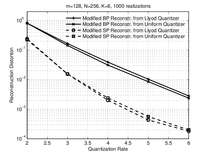
We performed extensive computer simulations in order to compare the performance of different quantizers and different reconstruction algorithms empirically. The parameters used in our simulations are m=128m=128, N=256N=256 and K=6K=6. Given these parameters, we generated realizations of m×Nm\times N sampling matrices from the i.i.d. standard Gaussian ensemble and normalize the columns to have unit l2l_{2}-norm. We also selected a support set TT of size |T|=K\left|T\right|=K uniformly at random, generated the entries supported by TT from the standard i.i.d. Gaussian distribution and set all other entries to zero. We let the quantization rates vary from two to six bits. For each quantization rate, we used Lloyd’s algorithm (Section II-B) to obtain a nonuniform quantizer and employed brute-force search to find the optimal uniform quantizer. To test different quantizers and reconstruction algorithms, we randomly generated 𝚽\mathbf{\Phi} and 𝐱\mathbf{x} independently a thousand times. For each realization, we calculated the measurements 𝐘\mathbf{Y}, the quantized measurements 𝐘^\hat{\mathbf{Y}} and the reconstructed signal 𝐗^\hat{\mathbf{X}}.

Fig. 1 compares uniform and uniform quantizers with respect to measurement distortion. Though the quantization rates in our experiments are relatively small, the simulation results are consistent with the asymptotic results in Theorem 1: nonuniform quantization is better than uniform quantization and the gain increases with the quantization rate. Fig. 2a compares the reconstruction distortion of the standard BP and SP algorithms. The comparison of the modified algorithms is given in Fig. 2. The modified algorithms reduce the reconstruction distortion significantly. When the quantization rate is six bits, the reconstruction distortion of the modified algorithms is roughly one tenth of that of the standard algorithms. Furthermore, for both the standard and modified algorithms, the reconstruction distortion given by SP algorithms is much smaller than that of BP methods. Note that the computational complexity of the SP algorithms is also smaller than that of the BP methods, which shows clear advantages for using SP algorithms in conjunction with quantized CS data. An interesting phenomenon occurs for the case of the modified BP method: although nonuniform quantization gives smaller measurement distortion, the corresponding reconstruction distortion is actually slightly larger than that of uniform quantization. We do not have solid analytical arguments to completely explain this somewhat counter-intuitive fact.

-A Proof of Theorem 1

Let T={1≤j≤N:Xj≠0}T=\left\{1\leq j\leq N:\;X_{j}\neq 0\right\} be the support set of 𝐱\mathbf{x}, i.e., xi≠0x_{i}\neq 0 for all i∈Ti\in T and xj=0x_{j}=0 for all j∉Tj\notin T. It is easy to show that for all 1≤i≤m1\leq i\leq m and T⊂{1,⋯,N}T\subset\left\{1,\cdots,N\right\} such that |T|=K\left|T\right|=K,

E⁡[∑j∈TAi,j​Xj]=0\mathrm{E}\left[\sum_{j\in T}A_{i,j}X_{j}\right]=0

and

E⁡[(∑j∈TAi,j​Xj)2]=K.\mathrm{E}\left[\left(\sum_{j\in T}A_{i,j}X_{j}\right)^{2}\right]=K.

According to the Central Limit Theorem, the distribution of 1K​∑j∈TAi,j​Xj\frac{1}{\sqrt{K}}\sum_{j\in T}A_{i,j}X_{j} converges weakly to the standard Gaussian distribution as K→∞K\rightarrow\infty. This can be verified by the facts that Ai,j​XjA_{i,j}X_{j}s are independent and identically distributed, and that the moment generating function of Ai,j​XjA_{i,j}X_{j} is well defined. As a result, the distribution of mK​Yi\sqrt{\frac{m}{K}}Y_{i} converges weakly to the standard Gaussian distribution as K,m,N→∞K,m,N\rightarrow\infty.

We apply a scalar quantizer with 2R2^{R} levels to the random variable mK​Yi\sqrt{\frac{m}{K}}Y_{i}. In this case, one has

1K​E​[‖𝐘^−𝐘‖22]\displaystyle\frac{1}{K}\mathrm{E}\left[\left\|\hat{\mathbf{Y}}-\mathbf{Y}\right\|_{2}^{2}\right]
=1m​mK​E​[∑i=1m(Y^i−Yi)2]\displaystyle=\frac{1}{m}\frac{m}{K}\mathrm{E}\left[\sum_{i=1}^{m}\left(\hat{Y}_{i}-Y_{i}\right)^{2}\right]
=1m​∑i=1mE⁡[(mK​Y^i−mK​Yi)2]\displaystyle=\frac{1}{m}\sum_{i=1}^{m}\mathrm{E}\left[\left(\sqrt{\frac{m}{K}}\hat{Y}_{i}-\sqrt{\frac{m}{K}}Y_{i}\right)^{2}\right]
=E⁡[(mK​Y^i−mK​Yi)2],\displaystyle=\mathrm{E}\left[\left(\sqrt{\frac{m}{K}}\hat{Y}_{i}-\sqrt{\frac{m}{K}}Y_{i}\right)^{2}\right], (29)

where the last line represents the distortion of quantizing mK​Yi\sqrt{\frac{m}{K}}Y_{i}. Note that the distortion-rate function for scalar quantization of a Gaussian random variable is given by

limR→∞​22​R​Dg∗​(R)=π​32​σ2,\underset{R\rightarrow\infty}{\lim}2^{2R}D_{g}^{*}\left(R\right)=\frac{\pi\sqrt{3}}{2}\sigma^{2}, (30)

where σ2\sigma^{2} is the variance of the underlying Gaussian source (see [18] for a detailed proof of this result). We then have

limR→∞​lim(K,m,N)→∞​22​RK​D∗​(R)=limR→∞​22​R​Dg∗​(R)=π​32,\underset{R\rightarrow\infty}{\lim}\;\underset{\left(K,m,N\right)\rightarrow\infty}{\lim}\frac{2^{2R}}{K}D^{*}\left(R\right)=\underset{R\rightarrow\infty}{\lim}2^{2R}D_{g}^{*}\left(R\right)=\frac{\pi\sqrt{3}}{2},

which completes the proof of (13).

Consider a uniform quantizer with codebook 𝒞u\mathcal{C}_{u}, such that |𝒞u|=2R\left|\mathcal{C}_{u}\right|=2^{R}, and apply the corresponding uniform quantizer to the random variable mK​Yi\sqrt{\frac{m}{K}}Y_{i}. It was shown in [19] that the distortion-rate function of uniform scalar quantizers of a Gaussian random variable equals

limR→∞​22​RR​Du,g∗​(R)=43​σ2​log⁡2.\underset{R\rightarrow\infty}{\lim}\frac{2^{2R}}{R}D_{u,g}^{*}\left(R\right)=\frac{4}{3}\sigma^{2}\log 2. (31)

It is clear that

limR→∞​lim(K,m,N)→∞​22​RK​R​Du∗​(R)=limR→∞​22​RR​Du,g∗​(R)=43​log⁡2,\underset{R\rightarrow\infty}{\lim}\;\underset{\left(K,m,N\right)\rightarrow\infty}{\lim}\frac{2^{2R}}{KR}D_{u}^{*}\left(R\right)=\underset{R\rightarrow\infty}{\lim}\frac{2^{2R}}{R}D_{u,g}^{*}\left(R\right)=\frac{4}{3}\log 2,

This proves Theorem 1.

-B Proof of Theorems 2 and 4

For completeness, let us first briefly review the key results used for deriving the asymptotic distortion-rate function for CS vector quantization. Suppose the source 𝐘∈ℝk\mathbf{Y}\in\mathbb{R}^{k} has probability density function f⁡(𝐲)f\left(\mathbf{y}\right). Let ℛ⊂ℝk\mathcal{R}\subset\mathbb{R}^{k} be a quantization region and 𝝎∈𝒞\bm{\omega}\in\mathcal{C} be the corresponding quantization level. The corresponding normalized moment of inertia (NMI) is defined as

m⁡(ℛ)=1k​∫ℛ‖𝐲−𝝎‖22​f​(𝐲)​𝑑𝐲(∫ℛ𝑑𝐲)1+2/k.m\left(\mathcal{R}\right)=\frac{\frac{1}{k}\int_{\mathcal{R}}\left\|\mathbf{y}-\bm{\omega}\right\|_{2}^{2}f\left(\mathbf{y}\right)d\mathbf{y}}{\left(\int_{\mathcal{R}}d\mathbf{y}\right)^{1+2/k}}.

The optimal NMI equals

mk∗=infℛ⊂ℝk​m​(ℛ),m_{k}^{*}=\underset{\mathcal{R}\subset\mathbb{R}^{k}}{\inf}m\left(\mathcal{R}\right),

only depends on the number of dimensions: mk∗=ckm_{k}^{*}=c_{k} with ck=112c_{k}=\frac{1}{12} when k=1k=1 and ck→12​π​ec_{k}\rightarrow\frac{1}{2\pi e} when k→∞k\rightarrow\infty. Thus the distortion rate function satisfies

limR→∞​2Rk​D​(R)\displaystyle\underset{R\rightarrow\infty}{\lim}\frac{2^{R}}{k}D\left(R\right) =∫f⁡(𝐲)λk2/k​(𝐲)​mk∗​𝑑𝐲,\displaystyle=\int\frac{f\left(\mathbf{y}\right)}{\lambda_{k}^{2/k}\left(\mathbf{y}\right)}m_{k}^{*}d\mathbf{y}, (32)

where RR is the quantization rate per dimension, and λk​(𝐲)\lambda_{k}\left(\mathbf{y}\right) denotes the point density function. In this case, the integral

∫ℳλk​(𝐲)​𝑑𝐲\int_{\mathcal{M}}\lambda_{k}\left(\mathbf{y}\right)d\mathbf{y}

gives the fraction of quantization levels belonging to ℳ\mathcal{M} for all measurable sets ℳ⊂ℝk\mathcal{M}\subset\mathbb{R}^{k}. For simplicity, we have assumed that λk​(𝐲)\lambda_{k}\left(\mathbf{y}\right) is continuous on ℝk\mathbb{R}^{k}. For fixed mk∗m_{k}^{*}, the problem of designing an asymptotically optimal quantizer can be reduced to the problem of finding the point density function λk∗​(𝐲)\lambda_{k}^{*}\left(\mathbf{y}\right) that minimizes (32). By Hölder’s inequality, the optimal point density function is given by

λk∗​(𝐲)=fk/(k+2)​(𝐲)∫fk/(k+2)​(𝐲)⋅𝑑𝐲,\lambda_{k}^{*}\left(\mathbf{y}\right)=\frac{f^{k/\left(k+2\right)}\left(\mathbf{y}\right)}{\int f^{k/\left(k+2\right)}\left(\mathbf{y}\right)\cdot d\mathbf{y}},

and the asymptotic distortion rate function is therefore

limR→∞​2Rk​D∗​(R)\displaystyle\underset{R\rightarrow\infty}{\lim}\frac{2^{R}}{k}D^{*}\left(R\right) =ck​(∫fk/(k+2)​(𝐲)⋅𝑑𝐲)k+2k.\displaystyle=c_{k}\left(\int f^{k/\left(k+2\right)}\left(\mathbf{y}\right)\cdot d\mathbf{y}\right)^{\frac{k+2}{k}}. (33)

If the source 𝐘\mathbf{Y} is Gaussian distributed with covariance matrix 𝚺>0\mathbf{\Sigma}>0, then the asymptotic distortion rate function (33) can be explicitly evaluated as

limR→∞​2Rk​D∗​(R)\displaystyle\underset{R\rightarrow\infty}{\lim}\frac{2^{R}}{k}D^{*}\left(R\right) =ck​|2​π​𝚺|1k​(k+2k)k+22\displaystyle=c_{k}\left|2\pi\mathbf{\Sigma}\right|^{\frac{1}{k}}\left(\frac{k+2}{k}\right)^{\frac{k+2}{2}} (34)
=|𝚺|1k​(1+oK​(1)),\displaystyle=\left|\mathbf{\Sigma}\right|^{\frac{1}{k}}\left(1+o_{K}\left(1\right)\right),

where oK​(1)→0o_{K}\left(1\right)\rightarrow 0 as K→∞K\rightarrow\infty, and the last equality follows from the fact that ck→12​π​ec_{k}\rightarrow\frac{1}{2\pi e} and (k+22)k+22→e\left(\frac{k+2}{2}\right)^{\frac{k+2}{2}}\rightarrow e as k→∞k\rightarrow\infty.

We present next the key results used for proving the upper bounds in (17) and (21).

Proposition 1

Let 𝐘0∈ℝk\mathbf{Y}_{0}\in\mathbb{R}^{k} be a Gaussian random vector with zero mean and covariance matrix 𝚺0\mathbf{\Sigma}_{0}. Let {𝔮R​(⋅)}\left\{\mathfrak{q}_{R}\left(\cdot\right)\right\}, where the subscript RR denotes the quantization rate, be a sequence of quantizers designed to achieve the asymptotic distortion rate function for Gaussian source 𝒩⁡(𝟎,𝚺1)\mathcal{N}\left(\mathbf{0},\mathbf{\Sigma}_{1}\right) with 𝟎<𝚺1∈ℝk×k\mathbf{0}<\mathbf{\Sigma}_{1}\in\mathbb{R}^{k\times k}. Apply 𝔮R​(⋅)\mathfrak{q}_{R}\left(\cdot\right) to 𝐘0\mathbf{Y}_{0}. If 𝚺0<𝚺1\mathbf{\Sigma}_{0}<\mathbf{\Sigma}_{1}, then

limR→∞​22​Rk​EY0​[‖𝐘0−𝔮R​(𝐘0)‖22]\displaystyle\underset{R\rightarrow\infty}{\lim}\frac{2^{2R}}{k}\mathrm{E}_{Y_{0}}\left[\left\|\mathbf{Y}_{0}-\mathfrak{q}_{R}\left(\mathbf{Y}_{0}\right)\right\|_{2}^{2}\right]
≤ck​(2​π​𝚺1)1k​(k+2k)k+22.\displaystyle\leq c_{k}\left(2\pi\mathbf{\Sigma}_{1}\right)^{\frac{1}{k}}\left(\frac{k+2}{k}\right)^{\frac{k+2}{2}}. (35)
Proof:

First assume that 𝟎<𝚺0\mathbf{0}<\mathbf{\Sigma}_{0}. Let f0​(𝐲)f_{0}\left(\mathbf{y}\right) and f1​(𝐲)f_{1}\left(\mathbf{y}\right) be the probability density functions for 𝐘0\mathbf{Y}_{0} and 𝐘1\mathbf{Y}_{1}, respectively. Denote EY0​[‖𝐘0−𝔮R​(𝐘0)‖22]\mathrm{E}_{Y_{0}}\left[\left\|\mathbf{Y}_{0}-\mathfrak{q}_{R}\left(\mathbf{Y}_{0}\right)\right\|_{2}^{2}\right] by D⁡(R)D\left(R\right). It is clear that

limR→∞​2Rk​D​(R)\displaystyle\underset{R\rightarrow\infty}{\lim}\frac{2^{R}}{k}D\left(R\right)
=ck​∫f0​(𝐲)(λk,1∗​(𝐲))2/k​𝑑𝐲\displaystyle=c_{k}\int\frac{f_{0}\left(\mathbf{y}\right)}{\left(\lambda_{k,1}^{*}\left(\mathbf{y}\right)\right)^{2/k}}d\mathbf{y}
=ck​∫f0​(𝐲)f12/(k+2)​(𝐲)​𝑑𝐲⋅(∫f1k/(k+2)​(𝐲)​𝑑𝐲)2k.\displaystyle=c_{k}\int\frac{f_{0}\left(\mathbf{y}\right)}{f_{1}^{2/\left(k+2\right)}\left(\mathbf{y}\right)}d\mathbf{y}\cdot\left(\int f_{1}^{k/\left(k+2\right)}\left(\mathbf{y}\right)d\mathbf{y}\right)^{\frac{2}{k}}. (36)

We upper bound the first integral as follows

∫f0​(𝐲)f12/(k+2)​(𝐲)​𝑑𝐲\displaystyle\int\frac{f_{0}\left(\mathbf{y}\right)}{f_{1}^{2/\left(k+2\right)}\left(\mathbf{y}\right)}d\mathbf{y}
=|2​π​𝚺1|1k+2|2​π​𝚺0|1/2​∫exp⁡{−12​𝐲∗​(𝚺0−1−2k+2​𝚺1−1)​𝐲}​𝑑𝐲\displaystyle=\frac{\left|2\pi\mathbf{\Sigma}_{1}\right|^{\frac{1}{k+2}}}{\left|2\pi\mathbf{\Sigma}_{0}\right|^{1/2}}\int\exp\left\{-\frac{1}{2}\mathbf{y}^{*}\left(\mathbf{\Sigma}_{0}^{-1}-\frac{2}{k+2}\mathbf{\Sigma}_{1}^{-1}\right)\mathbf{y}\right\}d\mathbf{y}
=(a)​|2​π​𝚺1|1k+2|2​π​𝚺0|1/2​|2​π​𝚺0|1/2|𝐈k−2k+2​𝚺0​𝚺1−1|1/2\displaystyle\overset{\left(a\right)}{=}\frac{\left|2\pi\mathbf{\Sigma}_{1}\right|^{\frac{1}{k+2}}}{\left|2\pi\mathbf{\Sigma}_{0}\right|^{1/2}}\frac{\left|2\pi\bm{\Sigma}_{0}\right|^{1/2}}{\left|\mathbf{I}_{k}-\frac{2}{k+2}\bm{\Sigma}_{0}\bm{\Sigma}_{1}^{-1}\right|^{1/2}}
≤(b)​|2​π​𝚺1|1k+2​(k+2k)k2\displaystyle\overset{\left(b\right)}{\leq}\left|2\pi\bm{\Sigma}_{1}\right|^{\frac{1}{k+2}}\left(\frac{k+2}{k}\right)^{\frac{k}{2}}
=∫f1kk+2​(𝒙)​𝑑𝒙,\displaystyle=\int f_{1}^{\frac{k}{k+2}}\left(\bm{x}\right)d\bm{x}, (37)

where (a)\left(a\right) holds because

𝚺0−1−2k+2​𝚺1−1\displaystyle\mathbf{\Sigma}_{0}^{-1}-\frac{2}{k+2}\bm{\Sigma}_{1}^{-1}
=𝚺0−1​(𝐈k−2k+2​𝚺0​𝚺1−1)\displaystyle=\bm{\Sigma}_{0}^{-1}\left(\mathbf{I}_{k}-\frac{2}{k+2}\bm{\Sigma}_{0}\bm{\Sigma}_{1}^{-1}\right)
=[(𝐈k−2k+2​𝚺0​𝚺1−1)−1​𝚺0]−1,\displaystyle=\left[\left(\mathbf{I}_{k}-\frac{2}{k+2}\bm{\Sigma}_{0}\bm{\Sigma}_{1}^{-1}\right)^{-1}\bm{\Sigma}_{0}\right]^{-1},

and (b)\left(b\right) follows from the assumption 𝚺0<𝚺1\mathbf{\Sigma}_{0}<\mathbf{\Sigma}_{1}. Substituting (37) into (36), one obtains

limR→∞​2Rk​D​(R)\displaystyle\underset{R\rightarrow\infty}{\lim}\frac{2^{R}}{k}D\left(R\right)
≤ck​(∫f1k/(k+2)​(𝐲)​𝑑𝐲)k+2k\displaystyle\leq c_{k}\left(\int f_{1}^{k/\left(k+2\right)}\left(\mathbf{y}\right)d\mathbf{y}\right)^{\frac{k+2}{k}}
=ck​|2​π​𝚺1|1k​(k+2k)k+22,\displaystyle=c_{k}\left|2\pi\mathbf{\Sigma}_{1}\right|^{\frac{1}{k}}\left(\frac{k+2}{k}\right)^{\frac{k+2}{2}},

which will be used to prove the upper bounds in (17) and (21).

Suppose that |𝚺0|=0\left|\mathbf{\Sigma}_{0}\right|=0 (some of the eigenvalues of 𝚺0\mathbf{\Sigma}_{0} are zero). Since 𝚺0<𝚺1\mathbf{\Sigma}_{0}<\mathbf{\Sigma}_{1}, when ϵ>0\epsilon>0 is sufficiently small, we have 𝟎<𝚺ϵ:=𝚺0+ϵ​𝐈<𝚺1\mathbf{0}<\mathbf{\Sigma}_{\epsilon}:=\mathbf{\Sigma}_{0}+\epsilon\mathbf{I}<\mathbf{\Sigma}_{1}. Let fϵ​(𝐲)f_{\epsilon}\left(\mathbf{y}\right) be the probability density function of Gaussian vector with zero mean and variance 𝚺ϵ\mathbf{\Sigma}_{\epsilon}. Then,

limR→∞​2Rk​D​(R)\displaystyle\underset{R\rightarrow\infty}{\lim}\frac{2^{R}}{k}D\left(R\right)
=ck​∫f0​(𝐲)(λk,1∗​(𝐲))2/k​𝑑𝐲\displaystyle=c_{k}\int\frac{f_{0}\left(\mathbf{y}\right)}{\left(\lambda_{k,1}^{*}\left(\mathbf{y}\right)\right)^{2/k}}d\mathbf{y}
=ck​∫limϵ→0​fϵ​(𝐲)(λk,1∗​(𝐲))2/k​𝑑𝐲\displaystyle=c_{k}\int\frac{\underset{\epsilon\rightarrow 0}{\lim}f_{\epsilon}\left(\mathbf{y}\right)}{\left(\lambda_{k,1}^{*}\left(\mathbf{y}\right)\right)^{2/k}}d\mathbf{y}
≤(c)​ck​liminfϵ→0​∫fϵ​(𝐲)(λk,1∗​(𝐲))2/k​𝑑𝐲\displaystyle\overset{\left(c\right)}{\leq}c_{k}\underset{\epsilon\rightarrow 0}{\lim\inf}\int\frac{f_{\epsilon}\left(\mathbf{y}\right)}{\left(\lambda_{k,1}^{*}\left(\mathbf{y}\right)\right)^{2/k}}d\mathbf{y}
≤(d)​ck​|2​π​𝚺1|1k​(k+2k)k+22,\displaystyle\overset{\left(d\right)}{\leq}c_{k}\left|2\pi\mathbf{\Sigma}_{1}\right|^{\frac{1}{k}}\left(\frac{k+2}{k}\right)^{\frac{k+2}{2}},

where (c)\left(c\right) follows from Fatou’s lemma [20], and (d)\left(d\right) follows from the first part of this proof. This proves the proposition. ∎

-B1 Lower Bounds for Scalar Quantization

We prove the lower bound in (17). Given Assumptions II, each YiY_{i}, 1≤i≤m1\leq i\leq m, is a linear combination of Gaussian random variables, and therefore each YiY_{i} is a Gaussian random variable itself. For a given ii and a given TT, the mean and the variance of YiY_{i} are E⁡[Yi]=0\mathrm{E}\left[Y_{i}\right]=0 and σi,T2=E⁡[Yi2]=∑j∈Tφi,j2\sigma_{i,T}^{2}=\mathrm{E}\left[Y_{i}^{2}\right]=\sum_{j\in T}\varphi_{i,j}^{2}, respectively. The variance depends on the row index ii and the support set TT. We calculate the average variance across all rows and all support sets as

σ¯2\displaystyle\bar{\sigma}^{2} =1m​∑i=1m(1(NK)​∑T∑j∈Tφi,j2)\displaystyle=\frac{1}{m}\sum_{i=1}^{m}\left(\frac{1}{{N\choose K}}\sum_{T}\;\sum_{j\in T}\varphi_{i,j}^{2}\right)
=1m​1(NK)​∑T∑j∈T(∑i=1mφi,j2)\displaystyle=\frac{1}{m}\frac{1}{{N\choose K}}\sum_{T}\;\sum_{j\in T}\left(\sum_{i=1}^{m}\varphi_{i,j}^{2}\right)
=(a)1m1(NK)∑j=1N(∑T:j∈T‖𝝋j‖22)\displaystyle\overset{\left(a\right)}{=}\frac{1}{m}\frac{1}{{N\choose K}}\sum_{j=1}^{N}\left(\sum_{T:\;j\in T}\left\|\bm{\varphi}_{j}\right\|_{2}^{2}\right)
=(b)​1m​1(NK)​∑j=1N(N−1K−1)​‖𝝋j‖22\displaystyle\overset{\left(b\right)}{=}\frac{1}{m}\frac{1}{{N\choose K}}\sum_{j=1}^{N}{N-1\choose K-1}\left\|\bm{\varphi}_{j}\right\|_{2}^{2}
=(c)​Km​1N​∑j=1N‖𝝋j‖22\displaystyle\overset{\left(c\right)}{=}\frac{K}{m}\frac{1}{N}\sum_{j=1}^{N}\left\|\bm{\varphi}_{j}\right\|_{2}^{2}
=(d)​Km​μ1,\displaystyle\overset{\left(d\right)}{=}\frac{K}{m}\mu_{1}, (38)

where

(a)\left(a\right)

is obtained by exchanging the sums over TT and jj,

(b)\left(b\right)

holds because for any given 1≤j≤N1\leq j\leq N, there are (N−1K−1){N-1\choose K-1} many subsets TT containing the index jj,

(c)\left(c\right)

is due to the fact that (N−1K−1)/(NK)=K/N{N-1\choose K-1}/{N\choose K}=K/N,

(d)\left(d\right)

follows from the definition (15).

Suppose that one deals with the ideal case: the support set TT is known before taking the measurements; and for different values of ii and TT, we are allowed to use different quantizers. Given ii and TT, we apply the optimal quantizer for the Gaussian random variable mK​Yi\sqrt{\frac{m}{K}}Y_{i}, so that the quantization distortion of YiY_{i} satisfies

limR→∞​22​R​Di,T∗​(R)=π⁡(mK​σi,T2)2​3,\underset{R\rightarrow\infty}{\lim}2^{2R}D_{i,T}^{*}\left(R\right)=\frac{\pi\left(\frac{m}{K}\sigma_{i,T}^{2}\right)}{2}\sqrt{3},

which is a direct application of (33) with k=1k=1. Taking the average over all ii and all TT gives

limR→∞​1m​∑i=1mET​[22​R​Di,T∗​(R)]\displaystyle\underset{R\rightarrow\infty}{\lim}\frac{1}{m}\sum_{i=1}^{m}\mathrm{E}_{T}\left[2^{2R}D_{i,T}^{*}\left(R\right)\right]
=1m​∑i=1m1(TK)​∑T(limR→∞​22​R​Di,T∗​(R))\displaystyle=\frac{1}{m}\sum_{i=1}^{m}\frac{1}{{T\choose K}}\sum_{T}\left(\underset{R\rightarrow\infty}{\lim}2^{2R}D_{i,T}^{*}\left(R\right)\right)
=1m​1(TK)​∑i=1m∑T(π⁡(mK​σi,T2)2​3)\displaystyle=\frac{1}{m}\frac{1}{{T\choose K}}\sum_{i=1}^{m}\sum_{T}\left(\frac{\pi\left(\frac{m}{K}\sigma_{i,T}^{2}\right)}{2}\sqrt{3}\right)
=π​μ12​3,\displaystyle=\frac{\pi\mu_{1}}{2}\sqrt{3},

where the last equality follows from (38).

However, the support set TT is unknown before taking the measurements. Furthermore, the same quantizer has to be employed for different choices of ii and TT. Thus, for every RR, ii and TT, EYi​[mK​|Yi−Y^i|2]≥Di,T∗​(R)\mathrm{E}_{Y_{i}}\left[\frac{m}{K}\left|Y_{i}-\hat{Y}_{i}\right|^{2}\right]\geq D_{i,T}^{*}\left(R\right). As a result,

liminfR→∞​22​RK​ET​[EY​[‖𝐘^−𝐘‖22]]\displaystyle\underset{R\rightarrow\infty}{\lim\inf}\frac{2^{2R}}{K}\mathrm{E}_{T}\left[\mathrm{E}_{Y}\left[\left\|\hat{\mathbf{Y}}-\mathbf{Y}\right\|_{2}^{2}\right]\right]
=liminfR→∞​22​R(NT)​∑T1m​∑i=1mmK​EY​[(y^i−yi)2]\displaystyle=\underset{R\rightarrow\infty}{\lim\inf}\frac{2^{2R}}{{N\choose T}}\sum_{T}\frac{1}{m}\sum_{i=1}^{m}\frac{m}{K}\mathrm{E}_{Y}\left[\left(\hat{y}_{i}-y_{i}\right)^{2}\right]
≥liminfR→∞​22​R(NT)​∑T1m​∑i=1mDi,T∗​(R)\displaystyle\geq\underset{R\rightarrow\infty}{\lim\inf}\frac{2^{2R}}{{N\choose T}}\sum_{T}\frac{1}{m}\sum_{i=1}^{m}D_{i,T}^{*}\left(R\right)
=π​μ12​3.\displaystyle=\frac{\pi\mu_{1}}{2}\sqrt{3}.

Since the above derivation is valid for all KK, mm and NN, the claim in (17) holds.

The result in (18) for uniform quantizers can be proved using similar arguments. For the ideal case, given ii and TT, apply the optimal uniform quantizer for the standard Gaussian random variable to mK​yi\sqrt{\frac{m}{K}}y_{i}. The corresponding distortion rate function for this case was characterized in [19] and s given by

limR→∞​22​R​Du,i,T∗​(R)=43​σi,T2​ln⁡2.\underset{R\rightarrow\infty}{\lim}2^{2R}D_{u,i,T}^{*}\left(R\right)=\frac{4}{3}\sigma_{i,T}^{2}\ln 2.

Therefore,

liminfR→∞​22​RK​ET​[EY​[‖𝐘^−𝐘‖22]]\displaystyle\underset{R\rightarrow\infty}{\lim\inf}\frac{2^{2R}}{K}\mathrm{E}_{T}\left[\mathrm{E}_{Y}\left[\left\|\hat{\mathbf{Y}}-\mathbf{Y}\right\|_{2}^{2}\right]\right]
≥43​μ1​ln⁡2,\displaystyle\geq\frac{4}{3}\mu_{1}\ln 2,

which completes the proof of (18).

-B2 The Upper Bound for Scalar Quantization

By the definition of μ2\mu_{2} in (16), the variance of the Gaussian random variable mK​Yi\sqrt{\frac{m}{K}}Y_{i} is upper bounded by μ2\mu_{2} uniformly for all ii and all TT. For each quantization rate RR, we design the optimal quantizer for a Gaussian source with variance μ2\mu_{2} and apply this quantizer to quantize all components of 𝐘\mathbf{Y}. Using (35), one can show that the quantization distortion for all ii and TT satisfies

limsupR→∞​22​RK​ET​E𝐘​[‖𝐘^−𝐘‖22]\displaystyle\underset{R\rightarrow\infty}{\lim\sup}\frac{2^{2R}}{K}\mathrm{E}_{T}\mathrm{E}_{\mathbf{Y}}\left[\left\|\hat{\mathbf{Y}}-\mathbf{Y}\right\|_{2}^{2}\right]
≤π2​μ2​3,\displaystyle\leq\frac{\pi}{2}\mu_{2}\sqrt{3},

which proves the upper bound in (17).

-B3 The Lower Bound for Vector Quantization

The basic idea for proving the lower bound in (20) is similar to that behind (17). For each TT, a lower bound on the minimum achievable distortion is derived. The average distortion taken over all the sets TT serves as a lower bound of the overall distortion-rate function.

Suppose the ideal case where we have prior knowledge of T∈([N]K)T\in{\left[N\right]\choose K}. We study the distortion rate function for every given TT. The measurement vector 𝐘\mathbf{Y} is Gaussian distributed with zero mean and covariance matrix 𝚽T​𝚽T∗\mathbf{\Phi}_{T}\mathbf{\Phi}_{T}^{*}, where 𝚽T\mathbf{\Phi}_{T} consists of the columns of 𝚽\mathbf{\Phi} indexed by TT. The singular value decomposition of 𝚽T​𝚽T∗\mathbf{\Phi}_{T}\mathbf{\Phi}_{T}^{*} gives 𝐔T​𝚲T​𝐔T∗\mathbf{U}_{T}\mathbf{\Lambda}_{T}\mathbf{U}_{T}^{*}, where 𝐔T∈ℝm×m\mathbf{U}_{T}\in\mathbb{R}^{m\times m} has orthonormal columns and 𝚲T=diag⁡(λ1,λ2,⋯,λm)\mathbf{\Lambda}_{T}=\mathrm{diag}\left(\lambda_{1},\lambda_{2},\cdots,\lambda_{m}\right) is the diagonal matrix formed by the singular values λ1≥λ2≥⋯≥λm\lambda_{1}\geq\lambda_{2}\geq\cdots\geq\lambda_{m}. Note that λi​(𝚽T∗​𝚽T)=λi​(𝚽T​𝚽T∗)\lambda_{i}\left(\mathbf{\Phi}_{T}^{*}\mathbf{\Phi}_{T}\right)=\lambda_{i}\left(\mathbf{\Phi}_{T}\mathbf{\Phi}_{T}^{*}\right) for 1≤i≤K1\leq i\leq K. According to Assumption III.1, the measurement matrix 𝚽\mathbf{\Phi} satisfies the RIP with constant parameter δK\delta_{K} , which implies that 1−δK≤λi​(𝚽T∗​𝚽T)≤1+δK1-\delta_{K}\leq\lambda_{i}\left(\mathbf{\Phi}_{T}^{*}\mathbf{\Phi}_{T}\right)\leq 1+\delta_{K} for all 1≤i≤K1\leq i\leq K. It can be concluded that 1−δK≤λi≤1+δK1-\delta_{K}\leq\lambda_{i}\leq 1+\delta_{K} for 1≤i≤K1\leq i\leq K and λi=0\lambda_{i}=0 for K+1≤i≤mK+1\leq i\leq m. As a result, 𝚽T​𝚽T∗=𝐔T,K​𝚲T,K​𝐔T,K∗\mathbf{\Phi}_{T}\mathbf{\Phi}_{T}^{*}=\mathbf{U}_{T,K}\mathbf{\Lambda}_{T,K}\mathbf{U}_{T,K}^{*} where 𝐔T,K∈ℝm×K\mathbf{U}_{T,K}\in\mathbb{R}^{m\times K} contains the first KK columns of 𝐔T\mathbf{U}_{T} and 𝚲T,K∈ℝK×K\mathbf{\Lambda}_{T,K}\in\mathbb{R}^{K\times K} is the diagonal matrix formed by the KK largest singular values. Denote the matrix formed by the last m−Km-K columns of 𝐔\mathbf{U} by 𝐔T,K⟂\mathbf{U}_{T,K}^{\perp}: clearly, 𝐔T=[𝐔T,K|𝐔T,K⟂]\mathbf{U}_{T}=\left[\mathbf{U}_{T,K}|\mathbf{U}_{T,K}^{\perp}\right].

The best quantization strategy is to quantize 𝐘¯=𝐔T,K∗​𝐘\bar{\mathbf{Y}}=\mathbf{U}_{T,K}^{*}\mathbf{Y} so that no quantization bit is used for the “trivial signal” (𝐔T,K⟂)∗​𝐘\left(\mathbf{U}_{T,K}^{\perp}\right)^{*}\mathbf{Y}. It is clear that 𝐘¯∼𝒩⁡(𝟎,𝚲T,K)\bar{\mathbf{Y}}\sim\mathcal{N}\left(\mathbf{0},\mathbf{\Lambda}_{T,K}\right) and 𝟎<𝚲T,K\mathbf{0}<\mathbf{\Lambda}_{T,K}. The corresponding asymptotic distortion rate function is therefore

limR→∞​22​m​R/KK​DT∗​(R)\displaystyle\underset{R\rightarrow\infty}{\lim}\frac{2^{2mR/K}}{K}D_{T}^{*}\left(R\right) =(34)​cK​(2​π​𝚲T,K)1K​(K+2K)K+22\displaystyle\overset{\left(\ref{eq:DRF-point-density-Gaussian}\right)}{=}c_{K}\left(2\pi\mathbf{\Lambda}_{T,K}\right)^{\frac{1}{K}}\left(\frac{K+2}{K}\right)^{\frac{K+2}{2}}
≥(1−δK)​(1+oK​(1)),\displaystyle\geq\left(1-\delta_{K}\right)\left(1+o_{K}\left(1\right)\right),

where the 22​m​R/K2^{2mR/K} term comes from the fact that the total quantization rate m​RmR is used to quantize a KK-dimensional signal. Since this lower bound is valid for all T∈([N]K)T\in{\left[N\right]\choose K}, we have proved the lower bound in (20).

-B4 The Upper Bound for Vector Quantization

Let ϵ>0\epsilon>0 be a small constant. Let {𝔮R​(⋅)}\left\{\mathfrak{q}_{R}\left(\cdot\right)\right\} be a sequence of quantizers that approaches the asymptotic distortion rate function for quantizing 𝐘¯∼𝒩⁡(𝟎,(1+δK+ϵ)​𝐈m)\bar{\mathbf{Y}}\sim\mathcal{N}\left(\mathbf{0},\left(1+\delta_{K}+\epsilon\right)\mathbf{I}_{m}\right). To prove the upper bound in (21), apply the quantizer sequence {𝔮R​(⋅)}\left\{\mathfrak{q}_{R}\left(\cdot\right)\right\} to 𝐘\mathbf{Y}. For every T∈([N]K)T\in{\left[N\right]\choose K}, 𝐘∼𝒩⁡(𝟎,𝚽T​𝚽T∗)\mathbf{Y}\sim\mathcal{N}\left(\mathbf{0},\mathbf{\Phi}_{T}\mathbf{\Phi}_{T}^{*}\right). According to the Assumption III.1, 𝚽T​𝚽T∗<(1+δK+ϵ)​𝐈m\mathbf{\Phi}_{T}\mathbf{\Phi}_{T}^{*}<\left(1+\delta_{K}+\epsilon\right)\mathbf{I}_{m}. Applying Proposition 1, we have

limR→∞​22​Rm​E𝐘​[‖𝐘−𝔮R​(𝐘)‖22]\displaystyle\underset{R\rightarrow\infty}{\lim}\frac{2^{2R}}{m}\mathrm{E}_{\mathbf{Y}}\left[\left\|\mathbf{Y}-\mathfrak{q}_{R}\left(\mathbf{Y}\right)\right\|_{2}^{2}\right]
≤(1+δK+ϵ)​(1+oM​(1)).\displaystyle\leq\left(1+\delta_{K}+\epsilon\right)\left(1+o_{M}\left(1\right)\right).

The upper bound in (21) is proved by taking the limit ϵ↓0\epsilon\downarrow 0.

-C The Existence and Uniqueness of (𝐱~,𝐲~)\left(\tilde{\mathbf{x}},\tilde{\mathbf{y}}\right) in Equation (28)

Consider the optimization problem

min(𝐱,𝐲)∈ℝ|T|×ℛ𝐘^​‖𝐲−𝚽T​𝐱‖2,\underset{\left(\mathbf{x},\mathbf{y}\right)\in\mathbb{R}^{\left|T\right|}\times\mathcal{R}_{\hat{\mathbf{Y}}}}{\min}\;\left\|\mathbf{y}-\mathbf{\Phi}_{T}\mathbf{x}\right\|_{2}, (39)

which is equivalent to

min(𝐱,𝐲)∈ℝ|T|×ℛ𝐘^​‖[−𝚽T​𝐈]​[𝐱𝐲]‖22.\underset{\left(\mathbf{x},\mathbf{y}\right)\in\mathbb{R}^{\left|T\right|}\times\mathcal{R}_{\hat{\mathbf{Y}}}}{\min}\;\left\|\left[-\mathbf{\Phi}_{T}\;\mathbf{I}\right]\left[\begin{array}[]{c}\mathbf{x}\\ \mathbf{y}\end{array}\right]\right\|_{2}^{2}. (40)

Note that the objective function is convex and the constraint set is convex and closed. The optimization problem (40) has at least one solution. Note that the matrix [−𝚽T​𝐈]\left[-\mathbf{\Phi}_{T}\;\mathbf{I}\right] does not have full row-rank. Hence, the solution may not be unique: the set 𝒬\mathcal{Q} defined in (27) gives all the possible solutions, and is convex and closed.

Let 𝔓\mathfrak{P} be the projection function from ℝ|T|×ℝm\mathbb{R}^{\left|T\right|}\times\mathbb{R}^{m} to ℝm\mathbb{R}^{m}, i.e., 𝔓⁡((,,,))=𝐲\mathfrak{P}\left(\left(\mathbf{x},\mathbf{y}\right)\right)=\mathbf{y}. Since the set 𝒬\mathcal{Q} is convex, the set 𝔓⁡(𝒬)\mathfrak{P}\left(\mathcal{Q}\right) is also convex. The quadratic optimization problem

min𝐲∈𝔓⁡(𝒬)​‖𝐘^−𝐲‖2\underset{\mathbf{y}\in\mathfrak{P}\left(\mathcal{Q}\right)}{\min}\left\|\hat{\mathbf{Y}}-\mathbf{y}\right\|_{2}

has a unique solution. Denote this unique solution by 𝐲~\tilde{\mathbf{y}}. Furthermore, recall our assumption that 𝚽T\mathbf{\Phi}_{T} has full column rank. For any given 𝐲∈ℝm\mathbf{y}\in\mathbb{R}^{m}, the solution of

min𝐱∈ℝ|T|​‖𝐲−𝚽T​𝐱‖2\underset{\mathbf{x}\in\mathbb{R}^{\left|T\right|}}{\min}\;\left\|\mathbf{y}-\mathbf{\Phi}_{T}\mathbf{x}\right\|_{2}

is therefore unique. As a result, there exists a unique 𝐱~∈ℝ|T|\tilde{\mathbf{x}}\in\mathbb{R}^{\left|T\right|} such that (𝐱~,𝐲~)∈𝒬\left(\tilde{\mathbf{x}},\tilde{\mathbf{y}}\right)\in\mathcal{Q}. This establishes the existence and uniqueness of the point (𝐱~,𝐲~)\left(\tilde{\mathbf{x}},\tilde{\mathbf{y}}\right).

References

  • [1] D. Donoho, “Compressed sensing,” IEEE Trans. Inform. Theory, vol. 52, no. 4, pp. 1289–1306, 2006.
  • [2] E. Candès and T. Tao, “Decoding by linear programming,” Information Theory, IEEE Transactions on, vol. 51, no. 12, pp. 4203–4215, 2005.
  • [3] E. Candès, M. Rudelson, T. Tao, and R. Vershynin, “Error correction via linear programming,” in IEEE Symposium on Foundations of Computer Science (FOCS), pp. 295 – 308, 2005.
  • [4] E. J. Candès and T. Tao, “Near-optimal signal recovery from random projections: Universal encoding strategies?,” IEEE Trans. Inform. Theory, vol. 52, no. 12, pp. 5406–5425, 2006.
  • [5] W. Dai and O. Milenkovic, “Subspace pursuit for compressive sensing signal reconstruction,” IEEE Trans. Inform. Theory, accepted, 2008.
  • [6] D. Needell and J. A. Tropp, “CoSaMP: Iterative signal recovery from incomplete and inaccurate samples,” Appl. Comp. Harmonic Anal., accepted, 2008.
  • [7] E. J. Candès, J. K. Romberg, and T. Tao, “Stable signal recovery from incomplete and inaccurate measurements,” Comm. Pure Appl. Math., vol. 59, no. 8, pp. 1207–1223, 2006.
  • [8] E. Candès and J. Romberg, “Encoding the ℓp\ell_{p} ball from limited measurements,” Data Compression Conference, pp. 33–42, March 2006.
  • [9] P. Boufounos and R. Baraniuk, “Quantization of sparse representations,” Preprint, 2008.
  • [10] P. Boufounos and R. G. Baraniuk, “1-bit compressive sensing,” in Conf. on Info. Sciences and Systems (CISS), (Princeton, NJ), pp. 16–21, March 2008.
  • [11] V. Goyal, A. Fletcher, and S. Rangan, “Compressive sampling and lossy compression,” IEEE Signal Processing Magazine, vol. 25, pp. 48–56, March 2008.
  • [12] I. E. Nesterov, A. Nemirovskii, and Y. Nesterov, Interior-Point Polynomial Algorithms in Convex Programming. SIAM, 1994.
  • [13] S. Lloyd, “Least squares quantization in pcm,” Information Theory, IEEE Transactions on, vol. 28, pp. 129–137, Mar 1982.
  • [14] K. Sayood, Introduction to Data Compression. Morgan Kaufmann, 3rd edition ed., 2005.
  • [15] T. M. Cover and J. A. Thomas, Elements of Information Theory. John Wiley & Sons, 1st edition ed., 1991.
  • [16] M. Akcakaya and V. Tarokh, “On sparsity, redundancy and quality of frame representations,” pp. 951–955, June 2007.
  • [17] E. Ardestanizadeh, M. Cheraghchi, and A. Shokrollahi, “Bit precision analysis for compressed sensing,” Preprint, 2009.
  • [18] P. Zador, Development and evaluation of procedures for quantizing multivariate distributions. PhD thesis, Stanford University, Stanford, CA, 1964.
  • [19] D. Hui and D. Neuhoff, “Asymptotic analysis of optimal fixed-rate uniform scalar quantization,” IEEE Trans. Inform. Theory, vol. 47, pp. 957–977, Mar 2001.
  • [20] H. Royden, Real Analysis. Prentice Hall, 3 edition ed., 1988.
Refer to caption
Figure 1: Distortion in the measurements.
Refer to caption
(a) By standard reconstruction algorithms
Refer to caption
(b) By modified reconstruction algorithms
Figure 2: Distortion in the reconstruction signals.